3D MHD Modeling of the Gaseous Structure of the Galaxy: Setup and Initial Results.

Abstract

We show the initial results of our 3D MHD simulations of the flow of the Galactic atmosphere as it responds to a spiral perturbation in the potential. In our standard case, as the gas approaches the arm, there is a downward converging flow that terminates in a complex of shocks just ahead of the midplane density peak. The density maximum slants forward at high $z$, preceeded by a similarly leaning shock. The latter diverts the flow upward and over the arm, as in a hydraulic jump. Behind the gaseous arm, the flow falls again, generating further secondary shocks as it approaches the lower $z$ material. In cases with two arms in the perturbing potential, the gaseous arms tended to lie somewhat downstream of the potential minimum. In the four arm case, this is true at large $r$ or early evolution times. At smaller $r$, the gaseous arms follow a tighter spiral, crossing the potential maximum, and fragmenting into sections arranged on average to follow the potential spiral. Structures similar to the high $z$ part of the gaseous arms are found in the interarm region of our two-armed case, while broken arms and low column density bridges are present in the four-armed case. Greater structure is expected when we include cooling of denser regions.

We present three examples of what can be learned from these models. We compared the velocity field with that of purely circular rotation, and found that an observer inside the galaxy should see radial velocity deviations typically greater than $20\mbox{~{}km s}^{-1}$. Synthetic spectra, vertical from the midplane, show features at velocities $\approx-20\mbox{~{}km s}^{-1}$, which do not correspond to actual density concentrations. Placing the simulated observer outside the galaxy, we found velocity structure and arm corrugation similar to those observed in H$\alpha$ in NGC 5427.

1 INTRODUCTION.

Even though spiral structure is one of the most prominent features of disk galaxies, details of the spiral arms in our own Galaxy remain uncertain. Georgelin & Georgelin (1976) traced the spiral structure of the Milky Way using H II regions, and developed a model with four arms. More recent attempts concluded that the Milky Way might actually have a superposition of two and four arm structures, each one with different pitch angles, which might arise from different components of the galactic disk (Drimmel, 2000; Lépine, Mishurov & Dedikov, 2001), suggesting that the stellar and gaseous disks might not be tightly coupled. Similar behavior has been frequently observed in external galaxies (Puerari & Dottori, 1992; Grosbøl & Patsis, 1998, for example).

Roberts (1969) showed that the gas must generate a large scale shock in the presence of a spiral perturbation. It was proposed that the density enhancement induced by this shock might generate a sequence of molecular clouds and star formation downstream from the shock, which itself was associated with the strong dust lane observed in the inner region of the spiral arms in external galaxies. Two dimensional numerical models by Tubbs (1980) and Soukup & Yuan (1981) showed that the gas forms a vertical shock perpendicular to the plane of the galactic disk. The post-shock gas remained close to hydrostatic equilibrium, even with an adiabatic equation of state. Their results did not show vertical motions larger than $3\mbox{~{}km s}^{-1}$. In fact, the largest downflow they found was due to the pre-shock gas readjusting its vertical structure as it flows into the arm potential. Therefore, when H I observations on face-on galaxies showed extended velocity components with dispersions of the order of $20\mbox{~{}km s}^{-1}$, they were attributed to other phenomena, such as galactic fountains, a warping of the H I disk, or intermediate velocity clouds (Dickey, Hanson & Helou, 1990; Kamphuis & Briggs, 1992; Kamphuis & Sancisi, 1993).

Since then, we have realized that the ISM is thicker and with a higher pressure than previously thought. The pressure scale height has been found to be larger than the density scale height, and the non-thermal pressures (turbulent, magnetic and cosmic ray) are at least as large as the thermal component (Badhwar & Stephens, 1977; Reynolds, 1989; Boulares & Cox, 1990). Therefore, less compressible gas needs to be considered in order to generate more realistic models of the ISM. Such a medium, with a larger effective $\gamma$ (the ratio of the specific heats) would be more likely to display the vertical motions characteristic of a hydraulic jump. With this in mind, Martos & Cox (1998, MC) performed 2D MHD simulations of the flow of the gaseous disk and found diverse structures that differed from the vertical near-hydrostatics found in previous studies. In many cases, the gas moved up ahead of the stellar arm, sped up over it, and fell behind with large bulk velocity. Frequently, there was a downstream shock at higher $z$ as this downflow was arrested, sometimes resulting in secondary midplane density maxima.

The goal of our investigation is to extend calculations like those of MC to three dimensions, to a large fraction of the Galaxy, and to look for its possible observational signatures. In this paper, we present the early results of these simulations. In Section 2 we describe the numerical setup and the procedure to achieve the initial hydrostatic equilibrium, in Section 3 we describe the results of the simulations, in Section 4 we present three examples of synthetic observations that can be done with this type of simulation, and in Section 5 we present our conclusions.

2 THE NUMERICAL SETUP.

We performed 3D MHD simulations in polar coordinates using the code ZEUS (Stone & Norman, 1992a, b; Stone, Mihalas & Norman, 1992). This code solves the ideal MHD equations for an inviscid fluid with infinite conductivity in a fixed eulerian grid. For our standard case, the grid extends from 0 to 1 kpc in $z$, 3 to 11 kpc in $r$, and 0 to $2\pi/N$ in the azimuthal angle $\phi$ with 50, 80 and $200/N$ grid points in each respective direction, $N$ being the number of arms in each case. The boundaries in $r$ and $z$ are reflective, while those in $\phi$ are periodic.

2.1 Hydrostatics, Theory.

The azimuthally averaged gravitational potential used is model 2 from Dehnen & Binney (1998). Using this potential, we set up a hydrostatic interstellar medium based on the scheme introduced by York et al. (1982) and described in the appendix of Benjamin (2002). We extended the procedure to include the effects of an azimuthal magnetic field whose magnitude depends only on the density. Given a density profile in the midplane, an equation of state (isothermal, in our case) and a density-magnetic pressure relation, the density and rotation velocity are uniquely defined everywhere.

Define the function $G(\rho)$ as:

$$G(\rho)=\int\frac{d}{d\rho}(p_{T}+p_{B})\frac{d\rho}{\rho},$$ (1)

where $\rho$ is the density and $p_{T}$ and $p_{B}$ are the thermal and magnetic pressures, respectively. Vertical hydrostatics, $\partial(p_{T}+p_{B})/\partial z=-\rho\partial\Phi/\partial z$ where $\Phi$ is the gravitational potential, reduces via Equation 1 to:

$$\frac{\partial(G+\Phi)}{\partial z} = 0$$ (2)

$$\Rightarrow G[\rho(r,z)] = G[\rho(r,0)]+\Phi(r,0)-\Phi(r,z).$$ (3)

At any $z$, the velocity profile is given by the radial balance between the radial potential and pressure gradients, the magnetic tension and the centrifugal force:

$$\frac{v_{\phi}^{2}(r,z)}{r}=\frac{\partial\Phi}{\partial r}+\frac{1}{\rho(r,z)}\left[\frac{\partial}{\partial r}(p_{T}+p_{B})+\frac{2p_{B}(r,z)}{r}\right].$$ (4)

This balance can be reduced to:

$$\frac{\partial(G+\phi)}{\partial r}=\frac{v_{\phi}^{2}-2p_{B}/\rho}{r}=\frac{v_{\phi}^{2}-v_{A}^{2}}{r},$$ (5)

where $v_{A}$ is the Alfvén velocity. Provided that $\partial^{2}(G+\Phi)/\partial z\partial r=\partial^{2}(G+\Phi)/\partial r\partial z$, along with Equations 2 and 5, we have:

$$\frac{\partial(v_{\phi}^{2}-v_{A}^{2})}{\partial z} = 0$$ (6)

$$\Rightarrow v_{\phi}^{2}(r,z) = v_{\phi}^{2}(r,0)-v_{A}^{2}(r,0)+v_{A}^{2}(r,z).$$ (7)

Given the midplane density distribution, $\rho(r,0)$, the density off the plane is obtained by solving Equation 3 for $\rho(r,z)$, while $v_{\phi}(r,0)$ is obtained from Equation 4 evaluated at $z=0$, after which the equilibrium rotation speed at all other $z$ follows from Equation 7.

2.2 Hydrostatics, Implementation.

Martos & Cox (1998) performed their 2D MHD calculations of spiral arm structure using the vertical density distribution at the solar circle compiled by Boulares & Cox (1990), modified to have a slightly lower vertical scale height for the warm ionized component. We found that the vertical distribution can be reproduced fairly accurately with thermal and magnetic pressures as follows. The thermal component assumes a neutral gas with a constant temperature of $5700~{}^{\mbox{o}}\mbox{K}$ and an isothermal equation of state. The magnetic pressure is taken as:

$$p_{B}=1.75\times 10^{-12}\frac{n}{n+n_{c}}\mbox{~{}dyn}\mbox{~{}cm}^{-2},$$ (8)

where $n_{c}=0.04\mbox{~{}cm}^{-3}$. The form of the magnetic pressure is such that it has little gradient at high density, and is proportional to $\rho$ at low density. The former accomodates a dense thermally supported core near the midplane, while the latter leads to a higher but constant signal speed at low density, far off the plane.

With a helium abundance equal to 10% of the hydrogen abundance by number, the mean atomic mass is $(14/11)m_{H}$.

In our initial work, we wanted to explore a situation that was not so heavily dominated by magnetic pressure. We therefore raised the temperature to $10^{4}~{}^{\mbox{o}}\mbox{K}$ and reduced the magnetic pressure by a factor of 10, keeping $n_{c}=0.04\mbox{~{}cm}^{-3}$. The midplane density distribution was taken as exponential, with a radial scale length of 4 kpc and a density of $1.11\mbox{~{}cm}^{-3}$ at $r=8\mbox{~{}kpc}$.

When these parameters are introduced into the above formalism and the hydrostatics found, the vertical half disk column density at $r=8\mbox{~{}kpc}$ is $0.12\mbox{~{}kpc}\mbox{~{}cm}^{-3}$. Figure 1 shows the density, rotation velocity and magnetic field strength versus radius at the midplane, and versus $z$ at $r=8\mbox{~{}kpc}$. The midplane density varies by less than a factor of 10, while vertically the density drops nearly four orders of magnitude between the midplane and $z=1\mbox{~{}kpc}$, our present maximum height. At smaller radii, the vertical gravity is stronger and the density gradient in $z$ even larger, so that both the highest and lowest densities occur at the inner boundary. A curious feature is that at high $z$, the density increases with increasing radius: the disk “flares”.

The rotation velocity varies only slightly with radius, by less than $15\mbox{~{}km s}^{-1}$, and by much less with $z$, only about $1\mbox{~{}km s}^{-1}$ increase (as per Equation 7, higher Alfvén speed requires higher rotation rate at high $z$ in this approximation). The magnetic field strength varies only slowly with radius, and appears roughly Gaussian in $z$, with a flat region in the inner 200 pc of the thermal core.

We also report below on a case which has no magnetic field, in which the constant value of the temperature was taken as $2.5\times 10^{4}~{}^{\mbox{o}}\mbox{K}$. More precisely, the thermal pressure at a given density was taken as 2.5 times that of the previous run, because the above temperature was used inconsistently with assuming the gas was still neutral. This increase in thermal pressure was made in order to have a density distribution roughly similar to the magnetic case.

2.3 The Spiral Perturbation.

In addition to the axisymmetric potential, we used a spiral perturbation of fixed shape that rotates with $\Omega_{P}=12\mbox{~{}km s}^{-1}\mbox{~{}kpc}^{-1}$ and has a pitch angle of $15\deg$. Details are reported in Cox & Gómez (2002). All the simulation grid is inside corotation. The depth of the perturbation varies slightly in $r$, weakens in $z$ and has a sinusoidal profile in $\phi$; in the midplane, its corresponding mass density amplitude is $\approx 52\%$ of the disk component of the axisymmetric model at $r=8\mbox{~{}kpc}$, which provides a peak to valley potential difference of about $(30\mbox{~{}km s}^{-1})^{2}$. This mass contrast is consistent with K-band observations performed by Rix & Rieke (1993), Rix & Zaritsky (1995) and Kranz, Slyz & Rix (2001), who quote an arm/interarm contrast in density of old stars between 1.8 and 3 for a sample of spiral galaxies.

2.4 Numerical Complications.

In early runs, performed with outflow boundary conditions at the inner, outer and upper boundaries, ZEUS soon reported difficulties with “hot zones” in which the timestep became so short that the calculation terminated. This is almost certainly caused by the enormous density contrast of our hydrostatic solution. By making those three boundaries reflecting, so that the material is unable to flow off the grid, this problem was postponed or eliminated, depending on the case run. The two arm magnetized case ran to about 270 Myr, the unmagnetized case and the four arm magnetized case ran the full 400 Myr asked of them.

In addition to changing the boundary conditions, we also changed the perturbation force field near the inner boundary after noticing that the spiral potential was pushing material against the inner boundary, causing reflected waves that propagated outward. In order to avoid splashing against the inner-$r$ boundary, this perturbation is not applied in the inner 1 kpc of the grid, while it is smoothly turned on in the subsequent kpc. Thus, the useful computational grid runs from 5 to 11 kpc. Also, in order to diminish initial transient effects, the spiral perturbation is turned on gradually during the first 50 Myr. This short turn-on time undoubtedly creates part of the transient behavior and may have exaggerated some of the early velocity structure. Our intention is to make runs lasting so long that such transients have died out, and to report on that asymptotic behavior in future work.

We are wary of artifacts that might be caused by our boundary conditions and will continue to experiment with alternatives, including cases with lower overall density contrast that might allow open boundaries.

3 BEHAVIOR OF THE SIMULATIONS.

Our primary example is the two armed spiral with moderate (reduced from MC) magnetic pressure. Our calculation space was the upper half (in $z$) of half a circular disk, with periodic boundaries in $\phi$. The period of time for a mass element to rotate around this half disk, relative to the rotating pattern, is about 100, 200 and 340 Myr ar $r=5,8$ and 10 kpc, respectively. We have chosen a fiducial time of 248 Myr, for our initial examination of the structure. At this time, nearly all mass elements have experienced the spiral perturbation once or twice, but conditions are still transient, representative of local interaction with rather than global accomodation to the perturbation. We will compare this early structure with that of the unmagnetized case at the same time, and the 4 arm magnetized case at half that time, which roughly represents the same level of maturity.

Having examined those single early time characteristics, we will present features of the subsequent development of the 2 arm cases and the much more mature 4 arm case, as indicative of features requiring a longer time to appear.

In the remainder of this paper, we will refer to each case using a three element naming scheme, describing the temperature (in units of $10^{4}~{}^{\mbox{o}}\mbox{K}$), the numerical coefficient in the magnetic pressure-density relation (Equation 8, in units of $10^{-12}\mbox{~{}dyn}\mbox{~{}cm}^{-2}$) and the number of spiral arms in the perturbation potential. Therefore, the magnetic two arm case will be denoted (1, 0.175, 2), the non-magnetic two arm case (2.5, 0, 2), and the four arm magnetic case (1, 0.175, 4).

3.1 Two Arm Magnetized Case.

Figures 2 and 3 show the results for the (1, 0.175, 2)  case. The lower panel shows the density and (in Figure 3) velocity field along a surface of constant radius $r=8\mbox{~{}kpc}$. The upper panel shows column density for $z\geq 0$, half the total. In the upper panel, rotation is clockwise, and in Figure 3, the lines show the integrated velocity field at the midplane. For clarity in the visualization, we modified the components of the velocity in the lower panel of this Figure, so the arrows representing velocity in the inertial reference frame are parellel to the flowlines, with relative lengths proportional to the total velocity.

The most important feature in Figure 2 and 3 is the presence of a simple grand design spiral. The density concentration in the midplane contains most of the column density. At higher $z$, this feature leans forward. The midplane gaseous arm appears slightly after the perturbation potential minimum (outward in radius), shifting to a better alignment farther above the plane (Figure 4). Note also the strong arm to interarm contrast; a significant fraction of the material is located in the arms. The convergences of the velocity flow field in the upper panel of Figure 3 are consistent with this concentration.

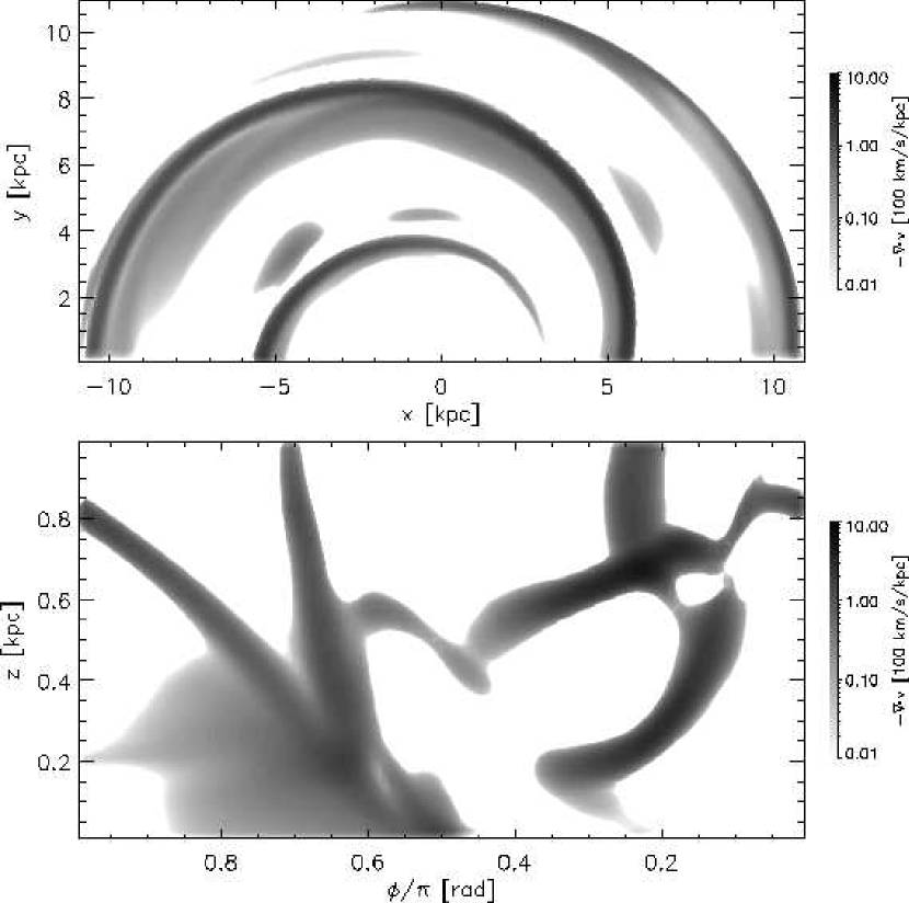
Figure 5: Divergence of the velocity for (1, 0.175, 2)  case at 248 Myr. Only those places with $\nabla\cdot\vec{v}<0$ are shown. The upper panel shows the midplane distribution, peaking at the inner edges of the column density arms of Figure 2. There is a substantial forward leaning shock (between $\phi/\pi=0.6$ and $0.7$) preceeding the forward leaning density ridge of Figure 2. (The high density at the base of the latter dominates the column density maps.) But there are a variety of other shocks as well.

Figure 5 shows the negative of the velocity divergence at the same positions as Figure 3. Only the regions with negative divergence are shown, in order to mark the places where strong compression (and shocks) appear. In the midplane, the compression of the material into the dense features is associated with a complex of intersecting shocks, following a diffuse compression of the material falling toward the arm. Comparison of Figures 3 and 5 shows an important shock 200 pc off the plane, preceding the gaseous arm, also slanting upstream at higher $z$. This shock accelerates gas upwards around $\phi/\pi\approx 0.6$. Over the arm, the flow is nearly horizontal. Behind the arm, it falls with vertical velocities of the order of $20\mbox{~{}km s}^{-1}$, forming secondary shocks. This behavior is more evident along the $\phi$-direction, but it is also visible in radial plots (not shown), since the presence of the stellar arms also induces velocities in that direction. Motions like these are similar to hydraulic jumps and were observed in the simulations performed by MC. MC also found midplane gas concentrations which they attributed to downstream bouncing of the flow. In our calculations, such concentrations are (so far) much smaller or absent in the midplane, but do appear in the lower density high $z$ gas, almost as if it tries to form another gaseous arm between the stellar arms. This interarm structure has little column density, but it is evident in the bottom panels of Figures 2 and 3, and the right hand panels of Figure 4.

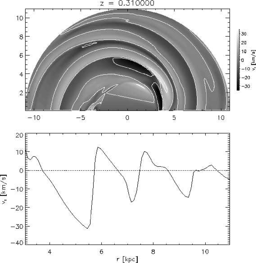
Figure 6: Vertical velocity structure at $z=.31\mbox{~{}kpc}$ for the (1, 0.175, 2)  case at 248 Myr. White contours in the upper panel are drawn at $v_{z}=-20,0\mbox{~{}and~{}}20\mbox{~{}km s}^{-1}$. Lower panel shows a cut along the vertical ($\phi=\pi/2$) line. Comparison of the upper panel with that of Figure 2 shows that the velocity field at this height has twice the frequency of the column density, i. e., it looks like a four arm spiral. The sawtooth pattern of the lower panel is consisntent with the velocity field of Figure 3 and $\nabla\cdot\vec{v}$ in Figure 5. There is a forward leaning shock (in $z$, see Figure 5) preceeding the forward leaning density ridge of the gaseous arm. Upstream from that shock, the gas is falling, downstream it is rising as in a hydraulic jump. Immediately over the arm, the vertical velocity is close to zero; gas flows up and over the density ridge and down the other side. As found by Martos & Cox (1998), the falling gas on the downstream side again shocks. In their case, this led to secondary density maxima in the midplane. In our runs thus far (e. g. Figure 4) there are secondary density maxima at high $z$, but they are too weak to show up in column density maps.

In Figure 6 we present the vertical velocity structure at 310 pc above the plane. The upper panel shows a gray scale of $v_{z}$ with contours at 0 and $\pm 20\mbox{~{}km s}^{-1}$. The gas moves up and over the gaseous structures at the arm and at the interarm positions, generating twice as many spirals in the upper panel of this Figure. Along the $\phi/\pi=0.5$ direction (lower panel), this behavior is clearer. While the arm is at $r\approx 8\mbox{~{}kpc}$ in this direction, the vertical velocity behaves similarly at 6 and 10 kpc. Notice that in all cases, the transition from downflow to upflow is sharp, while the downturn of the gas is much smoother.

3.2 Two Arm Unmagnetized and Four Arm Cases.

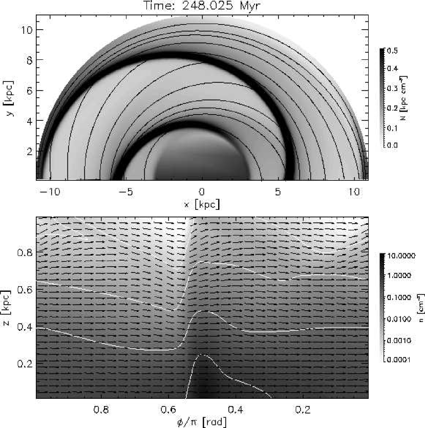
Figure 7: Same as Figure 3, but for the (2.5, 0, 2)  case. The temperature in this case is increased to $2.5\times 10^{4}~{}^{\mbox{o}}\mbox{K}$ in order to have a similar equilibrium density distribution without the magnetic field of the previous case. The arm shock and density ridge are more vertical and closer together than in the magnetized case, and the flow up and over the arms is less extreme. There is a weak shock at the upper right corner of the lower panel, roughly from $(\phi,z)=(.2,.8)$ through (0,.9), where the downflow bounces, but on the whole, the flow is much less structured, less like a hydraulic jump.

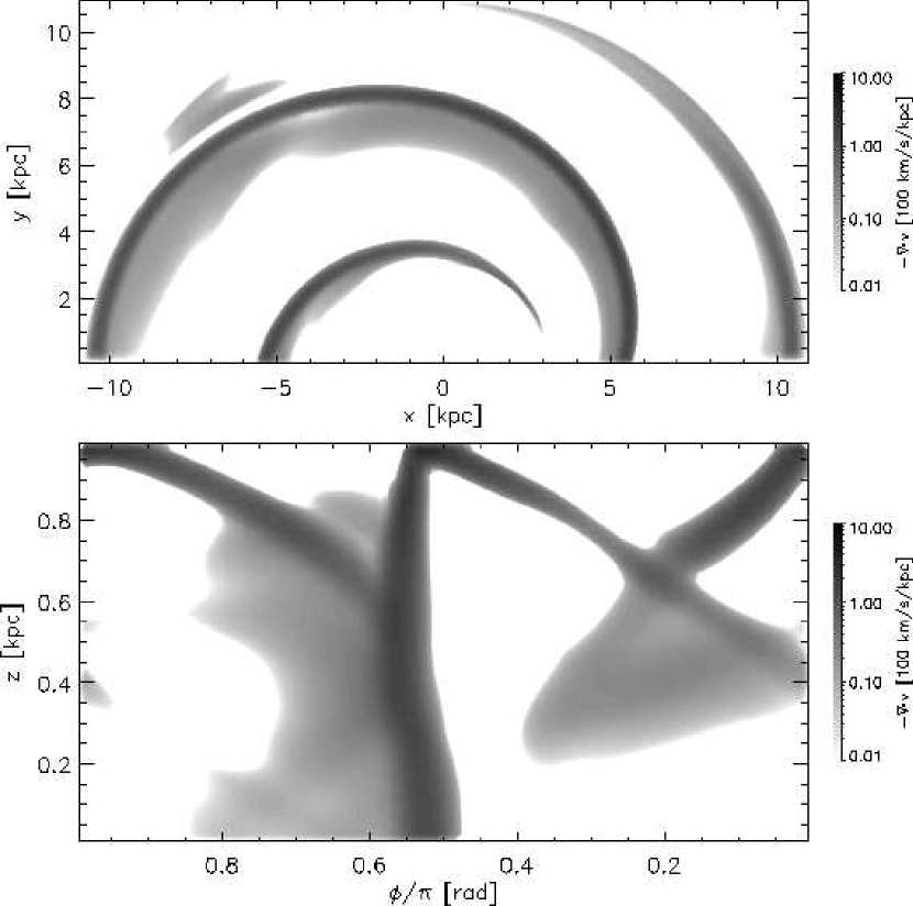
Figure 8: Divergence of the velocity for the (2.5, 0, 2)  case. Again, only those places with negative divergence are presented. Notice the presence of an important vertical shock just upstream from the gaseous arm. High-$z$ slanted shocks behind the arm like those observed in the magnetic case are also present here, but are weaker and may involve significant interaction with the closed upper boundary.

As a comparision, Figures 7 and 8 show the (2.5, 0, 2)  case at 248 Myr. Here, the temperature is higher in order to have a similar vertical density distribution. In the upper panel of Figure 7, we again observe the crowding of the midplane velocity field into the arms, as in Figure 3. The vertical structure now presents a strong shock at the leading edge of a nearly vertical gaseous arm and a much smoother density distribution behind it, which makes the gaseous arms fuzzier on the downstream side. There is vertical velocity structure, similar to the previous case, but with lower magnitude and only in the upper half of the grid.

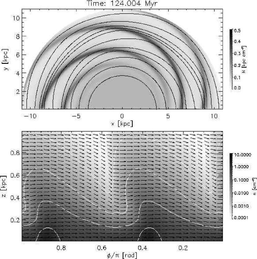
Figure 9: The same as Figure 3, but for the (1, 0.175, 4)  case at a time of 124 Myr. The gas, again, proceeds from left to right through the pattern. The earlier time was chosen so that the number of interactions with the arm potential would be similar, i. e. the flow is at a similar level of maturity. The flow in the reduced interarm space is considerably less complicated than that of the two arm case, apparently with insufficient time for an extra bounce. The column density in the arms is also lower because the concentration is so high that it matters that the material is being shared among four arms rather than two. Notice the substantial downflow preceeding the arm shock and the subsequent almost imperceptible upflow.

At 124 Myr, the four arm case (1, 0.175, 4)  in Figure 9 looks very similar to our standard case. Above 150 pc, strong downflows before the arms change suddenly to upflow at the arm position. In general, the column density is always smaller, since the same amount of mass is being distributed over 4 arms, leading to smaller arm to interarm contrast. This case is identical to the one presented in Figure 2, except for having 4 spiral arms perturbing the potential and that the grid covers only a quarter of the disk. We do not get interarm structures probably because there is not enough room between the arms for it.

Another difference between the four and two arm cases is that, for a given depth, the potential is steeper when four arms are present. Martos et al. (2002) developed a self-consistent model of the galactic spiral arms which resulted in narrower arms with a flat interarm region. They performed 1D MHD simulations with the usual sinusoidal potential and their modified perturbation, and found differences in the gaseous structures generated. The full 3D hydrodynamical effects of the details of the implementation of the perturbation potential will require further investigation.

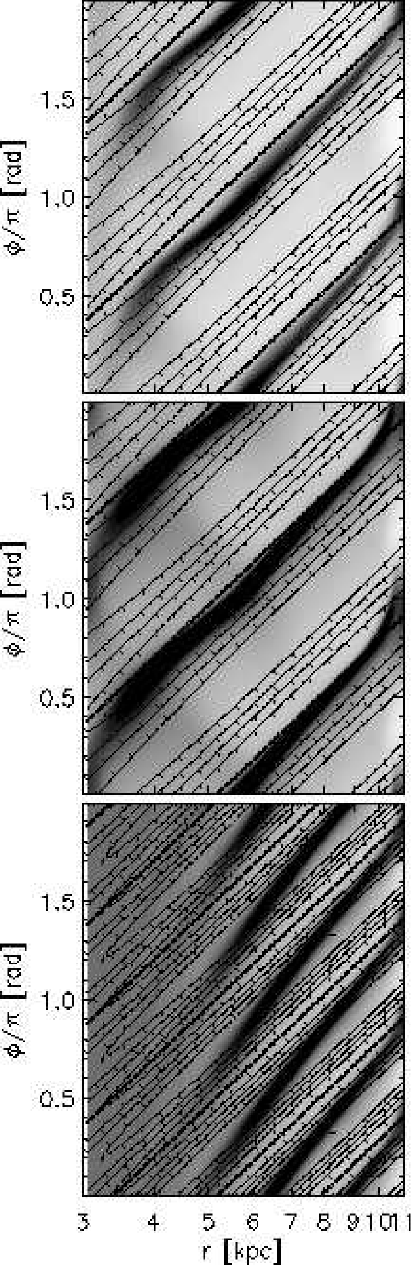
Figure 10: Comparison of the density structures and the spiral perturbation in $\log r-\phi$ space. In the three figures, the gray scales are column density, while the solid lines denote the spiral perturbation. Dotted lines show spirals with a pitch angle of $15\deg$ and run through the potential minima. In our trailing spiral model, the gas flows down from the top. From the top, panels correspond to the (1, 0.175, 2), (2.5, 0, 2)  and (1, 0.175, 4)  cases. Our potential perturbation is full strength only outward from 5 kpc. Notice that in the two arm cases the density concentrations appear downstream from the potential well, angling toward it with increasing $r$. The effect is so strong in the four arm case that the gaseous arm actually crosses the potential maximum (the stellar interarm). In all the cases the gas generates a spiral slightly tighter than that of the imposed potential.

A nice way to examine the phase between gaseous arms and the perturbing potential is by plotting column density in $\phi-\log(r)$ space, so that a logarithmic spiral appears as straight lines. Such plot is presented in Figure 10. Solid lines show contours of the underlying potential perturbation at the midplane, with the tick marks indicating the downhill direction. Dotted lines follow logarithmic spirals with pitch angle equal to the perturbation ($15\deg$), along the perturbation minima. Gray scale indicates column density in arbitrary units. As our model is of trailing spirals, the gas flows down from the top. In the (1, 0.175, 2)  (upper panel), and (2.5, 0, 2)  (middle panel) cases, the gaseous arms are slightly downstream from the potential minimum, by a gradually varying amount. The (1, 0.175, 4)  case (bottom panel), on the other hand, follows a tighter spiral with a pitch angle of about $12\deg$. Also, the gaseous arms do not extend as far into the inner radii. If this difference in pitch turns out to be a robust feature of future simulations, it would lead to differences in the characteristics of the spiral structure of galaxies when comparing observations of Pop II with H I or Pop I tracers (Drimmel, 2000, for example).

3.3 Cyclic Variation.

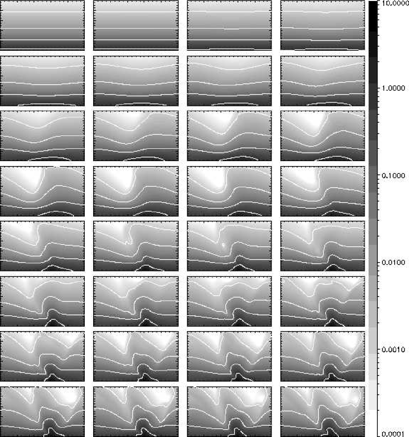
Figure 11: Time sequence of density slices for the (1, 0.175, 2)  case. Each panel corresponds to the lower panel of Figure 2, and there are 8 Myr between each slice. At high $z$ there is some indication of a “breaking-wave like” structure with a period of around 80 to 100 Myr. The period and structural details likely depend on the height (1 kpc) and type of the upper boundary (closed).

The runs presented here do not yet correspond to an asymptotic state, but it appears that they already have some cyclic behavior in the their evolution. Figure 11 presents the time sequence for the evolution of the (1, 0.175, 2)  case. Each panel corresponds to the lower panel in Figure 2, starting at t=0 with 8 Myr spacing. A high density structure above the arm is fully formed and leans upstream at $\approx 120\mbox{~{}Myr}$. It then contracts back as material from the tip falls down ($t\approx 168\mbox{~{}Myr}$), only to rise again from behind the arm, as in a breaking wave. Although it is hard to see in this Figure, such behavior is evident in an animation. The interarm structure (at the left side of the plots) also shows such cycles, with approximately the same phase. The reader must keep in mind that the gas making these structures is constantly moving around the galaxy and, therefore, these motions are really density waves on top of the galactic rotation. These cycles show a period of approximately 80 to 100 Myr. The (1, 0.175, 4)  case presents a similar behavior, with a slightly longer period. The (2.5, 0, 2)  case also presents such a cyclic variation, although it is less prominent. In all cases, the behavior is superposed on secular evolution in the arm structures.

3.4 Later Stages.

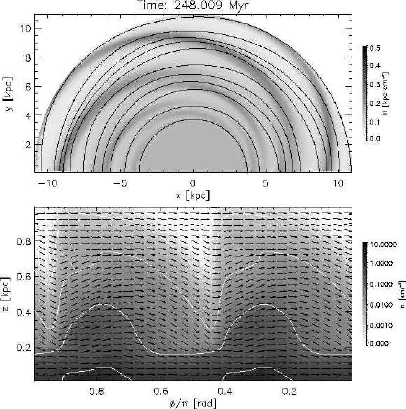
Figure 12: (1, 0.175, 4)  case at 248 Myr. Notice the formation of feathered arms inside 7 kpc. The lower panel (at $r=8\mbox{~{}kpc}$) shows some qualitative changes from Figure 9. The density contours drop more abruptly on the downstream side, the vertical velocities are more pronounced, and the midplane density and total column density distributions are wider and more diffuse.

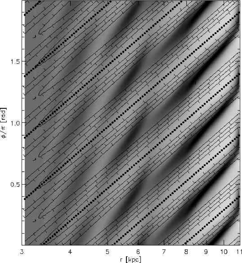
Figure 13: Same as Figure 10 but for the (1, 0.175, 4)  case at 248 Myr. Notice the formation of feathers inside $r=7\mbox{~{}kpc}$. The gaseous arms have locally shallower pitch than the perturbation but manage, by feathering, to achieve close to the same average pitch. The feathers lie along the interarm of the perturbing stellar arms.

Figure 12 show the (1, 0.175, 4)  case at 248 Myr. At this time, the gas has encountered the spiral arms twice as many times as in Figure 9. Fragmented arms are present inside $r=7\mbox{~{}kpc}$, while grand design arms are still present further out. A $\phi\mbox{~{}vs.~{}}\log(r)$ plot (Figure 13) shows the gaseous structures actually distributed along the potential maxima, instead of the minima. In the outer edges, the gaseous arms return to their previous position just downstream of the minimum. A time sequence of this case show that the gaseous arms drift downstream and stabilize at the potential crest. This evolution proceeds from the inner radii out. After a small section of the arms has drifted downstream, the arm breaks and the outer tip remains anchored at its original position. The result is that each individual section follows a tighter spiral, and the locus of all the sections, as a set, follow nearly the same spiral as the pertubation potential. Frequently, observations of the spiral structure in galaxies, even grand design spirals, show this type of feathering, in gaseous or Pop I tracers.

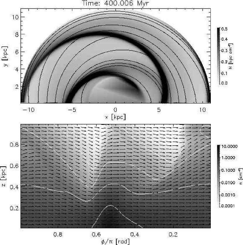
Figure 14: (2.5, 0, 2)  case at 400 Myr. Notice in the upper panel the formation of an interarm bridge in the inner galaxy, stretching between $r=4$ and 5 kpc. This is the regime in which the amplitude of the arm perturbation forces are increasing from zero to their full values. As with the (1, 0.175, 4)  case, the arm density structure has become somewhat more diffuse and the vertical velocity more pronounced, particularly in the interarm region ($\phi/\pi\approx 0.1$).

After 400 Myr, the (2.5, 0, 2)  case also starts developing an interarm structure at small radii (Figure 14), in this case a bridge between arms. As this entire structure is interior to 5 kpc, the smallest radius at which our perturbation forces are fully activated, this structure may be an artifact. The potential for this formation is already evident from the velocity field in the upper panel of Figure 7.

4 SYNTHETIC OBSERVATIONS.

When we have refined our models and followed them into asymptotic behavior, we will examine signatures to compare with observational data. Here, we present some preliminary examples of how our simulated galaxy would look to observers from within, and from the outside.

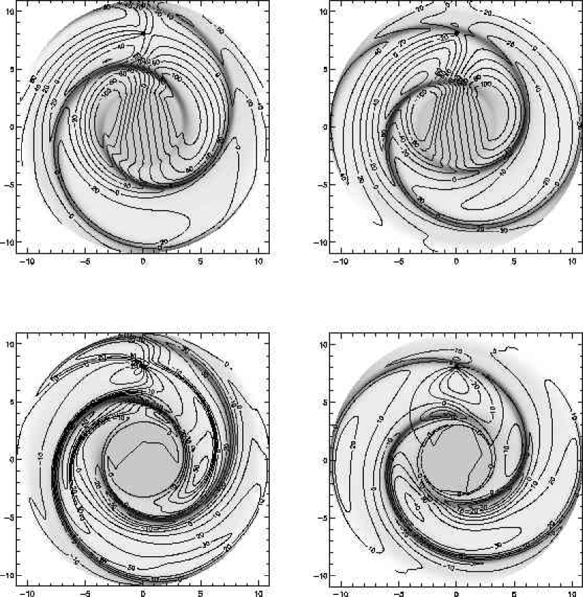
Figure 15: The upper panels show the line-of-sight component of the midplane velocity of the gas (in km/s) when the observer (at $x=0$, $y=8\mbox{~{}kpc}$) is at a interarm region (left panel) or near the inner region of an arm (right panel). The lower panels show the line-of-sight component of the deviation of those velocities from circular rotation. Notice that large velocity differences appear even at locations near the observer.

Gas velocities inconsistent with a circular galactic rotation have been routinely observed (see for example Tripp, Sembach & Savage 1993). In order to study the line-of-sight component of the non-circular motions in our modeled galaxy, we assigned a reference position in the midplane of the disk and calculated the radial velocity from it of all other midplane locations. Upper panels on Figure 15 show that radial component, while the lower panels show the velocity difference between it and a purely azimuthal rotation. The two cases are for an observer in an interarm region and one at the inner edge of a gaseous arm. The circular velocity considered was the solution to our hydrostatics equations discussed in Section 2. The velocity differences frequently exceed $20\mbox{~{}km s}^{-1}$, which would lead to errors in distance determinations of several kpc, even near the observer. Suggestion of problems in the determination of kinematic distances to pulsars have been found by Gómez et al. (2001). After tuning the input parameters in our simulation to a more realistic picture of the Milky Way, we will examine the degree to which those distance inconsistencies can be accounted for by considering non-circular gas motions.

Motions in the ISM are also observed in the form of intermediate velocity gas above the plane. In the simulations presented here, a large layer of gas falls behind the spiral arms (and sometimes, between them), all with similar speed. So, to an observer situated at the right position, this gas would appear as a falling velocity feature, a “cloud,” even without a localized density enhancement. Figure 16 shows this situation. After choosing a particular position in radius and azimuth, we interpolated the vertical distribution to a finer grid in order to generate a smooth artificial spectrum. All the spectra in the Figure correspond to $r=8\mbox{~{}kpc}$. Comparison with Figure 3 shows that the four azimuthal positions correspond to interarm, just before the arm, at the midplane density peak, and the downflow region after the arm. The two left hand panels show the characteristic upflow extending to about $5\mbox{~{}km s}^{-1}$, while the two right hand panels (and to a lesser extent, the lower left one) present an extended wing towards larger negative velocities, together with a small peak at about $-18\mbox{~{}km s}^{-1}$. As seen in Figure 6, the asymmetry in the velocity distribution appears because the upflow happens in a narrower region of higher density and lower velocity than the downflow. Therefore, just by chance, it is easier to pick a region in which the gas seems to be falling than one with upflowing gas, and the velocities are likely higher as well.

Our third example shows the appearance of our galaxy model from outside, in velocity resolved spectra of lines originating in the low density material well off the plane. Vertical motion of the gas have been found in H$\alpha$ observations of NGC 5427 by Alfaro et al. (2001). These motions are consistent with what would be expected by corrugation in the velocity field of the gaseous disk induced by a hydraulic jump around the spiral arms. Our simulations do not include the ionization structure of the gas (and could not without including the ionizing agents) but it is reasonable to expect that the lowest density regions will be ionized and that their behavior will approximate that of the warm ionized component of the interstellar medium and have a direct relation with H$\alpha$ observations. With this in mind, we simulated the study done by Alfaro et al. (2001) in Figure 17 using our (1, 0.175, 2)  case. The continous line is the integrated vertical velocity weighted by the square of the density,

$$w_{z}(r,\phi)=\frac{\sum_{z}v_{z}(r,\phi,z)\times[n(r,\phi,z)f(n)]^{2}}{\sum_{z}[n(r,\phi,z)f(n)]^{2}},$$ (9)

where $f(n)=1$ if $n\leq n_{lim}$, $f(n)=(n/n_{lim})^{-2.17}$ otherwise, and $n_{lim}=0.01\mbox{~{}cm}^{-3}$. The dotted line show the emission measure for these same grid points, defined as

$$EM=\sum_{z}[n(r,\phi,z)f(n)]^{2},$$ (10)

in arbitrary units. The midplane gaseous arm is at $r=8.5\mbox{~{}kpc}$. As observed by Alfaro et al. (2001), the gas moves up as it approaches the arm, falling behind it. A distinctive feature is that the EM peak is upstream from the gaseous arm at the midplane. Notice that the observations of NGC 5427 are for a region outside corotation, and therefore, the gas there moves from the convex to the concave sides of the gaseous arm, in the opposite direction from the gas in our simulation. In addition, the approximate $30\deg$ inclination angle for NGC 5427 should also show the imprint of radial streaming motions in the plane of the galaxy in this kind of observation.

Comparison of our Figures 3 and 17 with Figure 2 in Alfaro et al. (2001) shows that the H$\alpha$ profile of a spiral arm is more ragged than the model profile in higher density gas. While the column density plot in our Figure 3 is a smooth spiral, the H$\alpha$ emission measure in Figure 17 has many wiggles.

5 CONCLUSIONS AND FUTURE WORK.

In this work, we present our early results in the 3D MHD modeling of the large scale interaction of the ISM with a spiral potential. The presence of a thicker, more pressurized gaseous disk, together with the extra freedom the gas has in 3D simulations, allows the generation of density and velocity structures that previous work failed to reveal.

We confirmed and extended the work by MC, in which large scale vertical motions of the gas are an intrinsic feature of the response to the spiral perturbation. The downflow occurs along a much broader region and at higher velocities than the upflow. The falling gas can have large regions with a very similar vertical component, which translates into velocity crowding. In the present models, this gas appears as peaks at about $20\mbox{~{}km s}^{-1}$ in spectra taken directly up from the midplane. These motions are accompanied with rapid flow above the arms and similar “up and over” motions in the radial direction. So far, there are some hints that such motions might be occuring in NGC 5427 (Alfaro et al., 2001).

We also found significant differences in the midplane line-of-sight velocity distribution as compared with a purely circular rotation model. We think that the presence of streaming motions generated by the spiral arms must be considered when estimating the distance to elements of the ISM using their velocity as reference. In the future, when we obtain a more realistic model for the Milky Way, we may be able to provide a reasonable recipe for translating radial velocities and galactic longitude data to distance in a more reliable way.

Our models have a number of numerical simplifications (low resolution, closed boundaries, short run times) and omission of physical processes (heating and cooling of the gas, cosmic rays, self gravity, ionization, star formation or associated energy injection). Improvement on the run times and resolution will allow us to follow the structures to maturity, better examine cyclic features, explore substructure formation such as feathers, bridging and gaseous interarms, follow the magnetic field energy density and geometry to saturation, and to explore radial migrations of material and angular momentum. Addition of a more realistic equation of state to represent heating and cooling of the gas will allow the formation of truly dense regions. The interaction between magnetized flow and these regions may qualitatively alter the general arm structure, the velocity field and the complexity of the magnetic field configuration.

Our results show that failure to consider high $z$ and non-circular motions of the ISM associated just with the response to the spiral potential can easily lead to confusion when interpreting observational results. The study of the gaseous structure of the Milky Way and other galaxies require the consideration of three dimensional effects and a more realistic model of the nature of the ISM and its interaction with other dynamical elements of the system.

Figure 1: Initial state of the (1, 0.175, 2)  case. Cases are labeled with ($T/10^{4}~{}^{\mbox{o}}\mbox{K},~{}p_{mag}/10^{-12}\mbox{~{}dyn}\mbox{~{}cm}^{-2},N$), where $T$ is the temperature, $p_{mag}$ is the coefficient in Equation 8, and $N$ is the number of spiral arms. The gas is in hydrostatic and dynamical equilibrium in the vertical and radial directions with a temperature of $10^{4}~{}^{\mbox{o}}\mbox{K}.$ The density is presented assuming a mean particle mass $\mu=1.27m_{H}$.

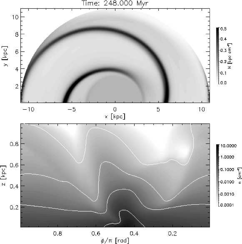
Figure 2: The upper panel shows the column density of the simulation for the (1, 0.175, 2)  case. The lower panel shows density along a cylindrical surface at $r=8\mbox{~{}kpc}$. White contours show density increasing in factors of 10, starting at $10^{-3}\mbox{~{}cm}^{-3}$.

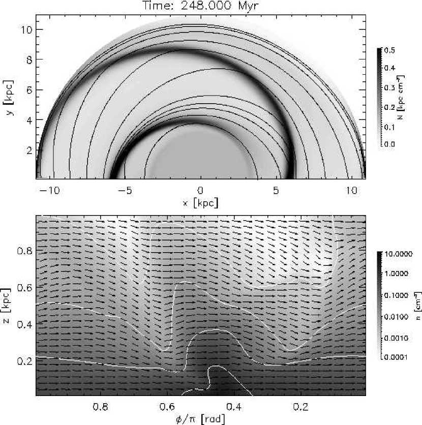
Figure 3: Same as Figure 2, with velocity structures superimposed. The continuous lines in the upper panel show the clockwise velocity field of the gas in the midplane. In the lower panel, the direction and relative length of the arrows is correct, but the length of the individual components is not. See discussion in the text.

Figure 4: Midplane perturbation potential, and density at different heights for the (1, 0.175, 2)  case at 248 Myr, along $\phi=\pi/2$ and $r=8\mbox{~{}kpc}$. Dotted lines show the initial (hydrostatic) density.

Figure 16: Simulated spectra for the (1, 0.175, 2)  case at $r=8\mbox{~{}kpc}$. The panels are picked trying to catch important features from Figure 3, namely an interarm region, at and around the gaseous arm. Even though most of the material sits near the plane, it is possible to obtain secondary peaks in velocity space that do not correspond to real gas concentrations in the physical space.

Figure 17: Synthetic H$\alpha$ observation of the model along $\phi=\pi/2$. This Figure is to be compared to Figure 2 in Alfaro et al. (2001). The solid line is the vertical velocity weighted with the square of the density for those grid-zones with $n<0.01\mbox{~{}cm}^{-3}$. It is similar in every feature to the vertical velocity at $z=0.31\mbox{~{}kpc}$ in Figure 6. The dotted line is the emission measure for the same positions. As the gas approaches the gaseous arm at 8.5 kpc, the flow rises to pass above it and then falls behind. Notice that the peak of the EM is upstream from the higher density gaseous arm in the midplane due to the forward lean of the arm at high $z$.

References

- Alfaro et al. (2001) Alfaro, E. J., Pérez, E., González Delgado, R. M., Martos, M. A., and Franco, J. 2001, ApJ, 550, 253
- Badhwar & Stephens (1977) Badhwar, G. D. and Stephens, S. A. 1977, ApJ, 212, 494
- Benjamin (2002) Benjamin, R. A. 2002 in preparation
- Boulares & Cox (1990) Boulares, A., and Cox, D. P. 1990, ApJ, 365, 544
- Cox & Gómez (2002) Cox, D. P. and Gómez, G. C. 2002, ApJS, submitted
- Dehnen & Binney (1998) Dehnen, W. and Binney, J. 1998, MNRAS, 294, 429
- Dickey, Hanson & Helou (1990) Dickey, J. M., Hanson, M. M. and Helou, G. 1990, ApJ, 352, 522
- Drimmel (2000) Drimmel, R. 2000, A&A, 358, L13
- Georgelin & Georgelin (1976) Georgelin, Y. M. and Georgelin, Y. P. 1976, A&A, 49, 57
- Gómez et al. (2001) Gómez, G. C., Benjamin, R. A. and Cox, D. P. 2001, ApJ, 122, 908
- Grosbøl & Patsis (1998) Grosbøl, P. J. and Patsis, P. A. 1998, A&A, 336, 840
- Kamphuis & Briggs (1992) Kamphuis, J. and Briggs, F. 1992, A&A, 253, 335
- Kamphuis & Sancisi (1993) Kamphuis, J. and Sancisi, R. 1993, A&A, 273, L31
- Kranz, Slyz & Rix (2001) Kranz, T., Slyz, A. and Rix, H.-W. 2001, ApJ, 562, 164
- Lépine, Mishurov & Dedikov (2001) Lépine, J. R. D., Mishurov, Y. N. and Dedikov, S. Y. 2001, ApJ, 546, 234
- Martos & Cox (1998) Martos, M. A. and Cox, D. P. 1998, ApJ, 509, 703 (MC)
- Martos et al. (2002) Martos, M. A., Pichardo, B., Moreno, E. and Espresate, J. 2002, ApJ, submitted
- Puerari & Dottori (1992) Puerari, I. and Dottori, H. A. 1992, A&AS, 93, 469
- Reynolds (1989) Reynolds, R. J. 1989, ApJ, 339, L29
- Rix & Rieke (1993) Rix, H.-W. and Rieke, M. J. 1993, ApJ, 418, 123
- Rix & Zaritsky (1995) Rix, H.-W. and Zaritsky, D. 1995, ApJ, 447, 82
- Roberts (1969) Roberts, W. W. 1969, ApJ, 158, 123
- Soukup & Yuan (1981) Soukup, J. E. and Yuan, C. 1981, ApJ, 256, 376
- Stone, Mihalas & Norman (1992) Stone, J. M., Mihalas, D. and Norman, M. L. 1992, ApJS, 80, 819
- Stone & Norman (1992a) Stone, J. M., and Norman, M. L. 1992a, ApJS, 80, 753
- Stone & Norman (1992b) Stone, J. M., and Norman, M. L. 1992b, ApJS, 80, 791
- Tripp, Sembach & Savage (1993) Tripp, T. M., Sembach, K. R. and Savage, B. D. 1993, ApJ, 415, 652
- Tubbs (1980) Tubbs, A. D. 1980, ApJ, 239, 882
- York et al. (1982) York, D. G., Songaila, A., Blades, J. C., Cowie, L. L., Morton, D. C. and Wu, C.-C. 1982, ApJ, 255, 467