Type Ia supernovae and the formation history of early-type galaxies

Abstract

Using the standard prescription for the rates of supernovae type II and type Ia, we compare the predictions of a simple model of star formation in galaxies with the observed radial gradients of abundance ratios in a sample of early-type galaxies to infer the relative contribution of each type of supernova. The data suggests a correlation between the fractional contribution of Type Ia to the chemical enrichment of the stellar populations ($1-\xi$) and central velocity dispersion of order $1-\xi\sim-0.16\log\sigma_{0}+0.40$, so that the type Ia contribution in stars ranges from a negligible amount in massive ($\sigma_{0}\sim 300$ km s^-1) galaxies up to $10\%$ in low-mass ($\sim 100$ km s^-1) elliptical galaxies. Our model is parametrized by a star formation timescale ($t_{\rm SF}$) which controls the duration of the starburst. A correlation with galaxy radius as a power law ($t_{\rm SF}\propto r^{\beta}$) translates into a radial gradient of the abundance ratios. The data implies a wide range of formation scenarios for a simple model that fixes the luminosity profile, ranging from inside-out ($\beta=2$), to outside-in formation ($\beta=-1$), as is consistent with numerical simulations of elliptical galaxy formation. An alternative scenario that links $t_{\rm SF}$ to the dynamical timescale favours inside-out formation over a smaller range $0.4<\beta<0.6$. In both cases, massive galaxies are predicted to have undergone a more extended period of star formation in the outer regions with respect to their low-mass counterparts.

1 Introduction

Type Ia supernovae (SNIa) describe stellar explosions whose spectra show lines of elements or intermediate mass such as silicon, and of the iron group, but no hydrogen lines. They currently occupy a very special place in cosmology since they can be used as standard candles. Even though their luminosities span an order of magnitude, empirical correlations between their absolute magnitude and the shape of their light curves can be used in order to determine distances (Phillips 1993) in an analogous way to classical Cepheids. Furthermore, the absolute luminosity of SNIa is orders of magnitude brighter than variable stars, enabling us to observe them at high redshift. This is a tool currently being used to constrain the cosmological parameters (e.g. Perlmutter et al. 1999; Riess et al. 1998). However, SNIa also play a very important role in the process of galactic chemical enrichment since they contribute a large amount of iron to the interstellar medium (Thielemann, Nomoto & Yokoi 1986). In fact Type Ia supernovae might even be the main producers of iron in the Universe (Ishimaru & Arimoto 1997; however see Gibson, Loewenstein & Mushotzky 1997). The observed properties of SNIa’s suggest a binary model in which at least one of the stars is a white dwarf that reaches the Chandrasekhar limit ($\sim 1.4M_{\odot}$) by accretion or by merging with another white dwarf. The timescale for the explosion is thereby limited by the lifetimes of stars which end up as white dwarfs, i.e. with masses $M\lower 2.15277pt\hbox{$\;\buildrel<\over{\sim}\;$}8M_{\odot}$. This implies that Type Ia’s can be observed long after star formation subsided. Indeed, all supernovae observed in early-type galaxies — which feature no ongoing star formation — are Type Ia, whereas late-type galaxies display a mixture of Type Ia and Type II supernovae (Cappellaro et al. 1997)

On the other hand, Type II supernovae (SNII) show hydrogen lines in their spectra and arise from the core collapse of a single, massive ($M\lower 2.15277pt\hbox{$\;\buildrel>\over{\sim}\;$}8M_{\odot}$) star at the end of its lifetime, which occurs between $1-50$ Myrs after the core hydrogen burning phase started. Hence, the timescales of either type of supernovae are remarkably different. Furthermore, the yields of chemical elements are also in sharp contrast, since SNIa produce much more iron than SNIIs, so that stars born during the first phases of star formation — when the contribution from SNIa to the interstellar medium was negligible — display an enhancement of $\alpha$ elements over iron, with respect to the younger generations of stars, such as the Sun, which are born in an environment polluted by both types of supernovae.

Observations of radial gradients in the colours (Franx, Illingworth & Heckman 1989; Peletier et al. 1990; Jørgensen, Franx & Kjægaard 1995) and line indices (González 1993; Davies, Sadler & Peletier 1993; Peletier et al. 1999) in elliptical galaxies show gradients, being mostly redder and more metal rich at their centres, although some early-type galaxies display blue cores (Menanteau, Abraham & Ellis 2001). Broadband photometry has been a technique repeatedly used to infer the star formation history of galaxies notwithstanding the age-metallicity degeneracy (Worthey 1994), which prevents us from getting a well-defined picture of galaxy formation using colours alone. A combined analysis of line indices seem to break the degeneracy since their age and metallicity dependence can be rather different (Kuntschner 2000; Trager et al. 2000a, 2000b). Abundance ratios represent an alternative observable since the timescales for SNIa and SNII are remarkably different. Giant early-type galaxies feature an overabundance of $\alpha$ elements over iron (Peletier 1989; Worthey, Faber & González 1992; Trager et al. 2000a; Kuntschner 2000), indicative of a short duration of the star formation stage, so that mostly SNII contribute to the metallicity of the stellar component.

This has been used in several models of galaxy formation in order to constrain the star formation history of galaxies. Matteucci (1994) analysed the observed [Mg/Fe] ratios in ellipticals to constrain the star formation history to timescales shorter than $0.1$ Gyr. Furthermore, the trend of [Mg/Fe] with galaxy mass was used to imply either an increasing star formation efficiency with galaxy mass, or a top-heavy initial mass function, so that more massive stars were formed in ellipticals compared to a more quiescent environment such as in a disk galaxy. A detailed analysis of abundance ratios in metal-poor stars is a valuable tool for determining the star formation history in the solar neighbourhood (Gratton et al. 2000), and this can be extended to stellar populations in globular clusters. In a recent analysis of abundance ratios in a sample of six red giant stars in the $\omega$ Cen cluster, Pancino et al. (2002) found evidence for the contribution of SNIa to the composition of younger, more metal rich red giants.

In this paper we explore the radial gradients observed in abundance ratios such as [Mg/Fe] in elliptical galaxies as a function of the star formation timescale. The relative contribution from SNIa and SNII can be compared with observations to infer the formation process of the stellar components, enabling us to connect the star formation history and the dynamical history of early-type galaxies. In §2 and §3 we describe the model used to predict the rates of either type of supernovae and their contribution to chemical enrichment. §4 describes our model predictions and compares them to observed data. Finally, in §5 we discuss the implications of the comparison between our simple model and the observed data.

2 Rates of type Ia and type II supernovae

The progenitors of type Ia supernovae are still a matter of debate. The most common candidates are either the double degenerate model (Iben & Tutukov 1984) in which two C-O white dwarfs merge, reaching the Chandrasekhar mass and exploding by C deflagration, and the single degenerate model (Whelan & Iben 1973) comprising a close binary system made of a nondegenerate star and a C-O white dwarf which accretes material from the other component, reaching the Chandrasekhar mass and triggering C deflagration. The negative result in the search for close binary systems made up of two massive white dwarfs in a sample of 54 white dwarfs (Bragaglia et al. 1990) hints at the single degenerate model as the most plausible one, which is the one we will assume henceforth. The ESO SNIa progenitor survey, which will use UVES/VLT (Koester et al. 2001) on a sample of 1,500 white dwarfs will clarify this point.

In order to estimate the rates of type Ia supernovae, we follow the prescription of Greggio & Renzini (1983), recently reviewed by Matteucci & Recchi (2001). The rate can be written as a convolution of the initial mass function (IMF) over the mass range that can generate a type Ia supernova. The lower mass limit is $M_{Bm}=3M_{\odot}$ in order to generate a binary with a white dwarf which will reach the Chandrasekhar limit. The upper mass limit is $M_{BM}=16M_{\odot}$ so that neither binary undergoes core collapse. The rate is thus:

$$R_{Ia}(t)={\cal A}\int_{3M_{\odot}}^{16M_{\odot}}dm\phi(m)\int_{\mu_{m}}^{\mu_{\rm max}}d\mu^{\prime}f(\mu^{\prime})\psi(t-\tau_{m_{2}}),$$ (1)

where $m_{t}={\rm max}(3M_{\odot},m(t))$ and $m(t)$ is the mass of a star whose lifetime is $t$, whereas $\tau_{m_{2}}$ is the lifetime of the nondegenerate companion, with mass $m_{2}$. $f(\mu)$ is the fraction of binaries with a mass fraction $\mu\equiv M_{2}/M_{B}$, where $M_{2}$ and $M_{B}$ are the masses of the secondary star and the binary system, respectively. The range of integration goes from $\mu_{m}={\rm max}(m_{2}/m,1-8M_{\odot}/m)$, to $\mu_{max}=0.5$. The analysis of Tutukov & Yungelson (1980) on a sample of about 1000 spectroscopic binary stars suggests that mass ratios close to $\mu=1/2$ are preferred, so that the normalized distribution function of binaries can be written:

$$f(\mu)=2^{1+\gamma}(1+\gamma)\mu^{\gamma},$$ (2)

as suggested by Greggio & Renzini (1983), and we adopt the value of $\gamma=2$. The normalization constant ${\cal A}$ is constrained by the ratio between type Ia and type II supernovae in our Galaxy that best fits the observed solar abundances. We use the result of Nomoto, Iwamoto & Kishimoto (1997), namely $R_{Ia}/R_{II}=0.12$ to find ${\cal A}=0.05$.

The rate of type II supernovae is also given as an integral of the star formation convolved with the IMF, in this case over the mass range expected for the precursors of single component supernovae, i.e. $8<M/M_{\odot}<50$. Here we adopt $50M_{\odot}$ as the upper mass cutoff. We use throughout the paper either a Salpeter (1955) or a Scalo (1986) IMF.

$$R_{II}(t)=\int_{8M_{\odot}}^{50M_{\odot}}dm\phi(m)\psi(t-\tau_{m}),$$ (3)

where we have neglected the contribution from binaries to the IMF over this mass range.

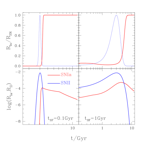
Figure 1: Relative contribution (top) and rates (bottom) of type Ia and type II supernovae for a generic star formation history described by a gaussian function peaked at $3$ Gyr with a star formation timescale of $t_{\rm SF}0.1$ (left) and $1$ Gyr, respectively.

Figure 1 shows the rates of either type of supernovae for a generic star formation history given by a gaussian profile with a width of $t_{\rm SF}=0.1$ Gyr (left panels) or $1$ Gyr, respectively. The shape of the curve plotting the rate of type IIs is nearly identical to the star formation rate given the very short lifetimes of massive stars that undergo core collapse. Hence, the rate of this type of supernovae is negligible a few Myr after the star formation has ceased. On the other hand, the longer timescales of the nondegenerate companions in type Ias imply that these supernovae start contributing significantly to the chemical enrichment of the ISM a few hundred Myr after the main burst of star formation. This effect is more extreme in sharply peaked bursts of star formation although its contribution to chemical enrichment is only important for the interstellar medium and not so much for the metallicities of the stellar populations unless later bursts of star formation allow the ejected metals from SNIas to be locked into subsequent generations of stars.

3 Chemical enrichment

The supernova rates allow us to infer the amount of metals ejected to the interstellar medium. We target magnesium and iron as the main elements which should be observed to discern the contribution between SNIa and SNII. Magnesium is one of the $\alpha$ elements, which are those that can be obtained from the reaction of C and O with helium nuclei. These elements are: Ne, Mg, Si, S. The solar abundance of these elements is slightly enhanced with respect to the mean (given by some average metallicity ${\cal Z}$). Another family of elements — the so-called iron-peak elements, which include Fe and Co — are less abundant with respect to ${\cal Z}$. Notice that the amount of iron-peak elements contributes only a small fraction to the total metallicity (8% at solar abundance), so that changing the abundance of Fe by a large amount does not affect significantly the average metallicity. Hence, it would be more correct to think of a depression in Fe-peak elements in solar abundances, rather than an enhancement of $\alpha$ elements at the centres of elliptical galaxies (Trager et al. 2000b).

The yields from SNIa are taken from the single degenerate model W7 of Thielemann et al. (1986), which assumes a progenitor made up of a $1M_{\odot}$, C$+$O white dwarf with equal parts of ¹²C and ¹⁶O, with an accretion rate of $4\times 10^{-8}M_{\odot}$ yr^-1. The yields from SNII are taken from Thielemann, Nomoto & Hashimoto (1996) for a range of progenitor masses. The stellar initial mass function (IMF) is used in order to take a weighted-average of the yields with respect to mass. The yields used in this paper are shown in Table 1. Notice that a very significant amount of iron is produced in SNIa with respect to the $\alpha$ elements. The mass contained in O-, Ne- and C-burning shells is too small compared with the mass in the Si-burning zone. This implies SNIa ejecta are dominated by the products of complete and incomplete Si-burning, i.e. a higher iron yield compared to the ejecta from core-collapse supernovae. However, this is still debatable because the yields may depend rather sensitively on the initial metallicity. For instance, assuming an average metallicity of $0.5{\cal Z}_{\odot}$ over the star formation history of the galaxy will lead to a total reduction of 25% in the amount of Fe ejected from SNIa (Thielemann et al. 1986).

TABLE 1: Supernovae yields (in $M_{\odot}$)

Type	Mg	$\alpha$	Fe	$[\alpha$/Fe$]$
SNIa	$0.016$	$0.438$	$0.742$	$-1.33$
SNII(Salpeter)	$0.122$	$3.177$	$0.094$	$+0.43$
SNII(Scalo)	$0.102$	$2.663$	$0.105$	$+0.30$

In this paper we do not consider the contribution of low and intermediate-mass stars ($M\leq 8M_{\odot}$) to chemical enrichment. We focus on the contribution from either type of supernova to the star formation history in early-type galaxies through the analysis of Mg and Fe. These elements are not produced in stars which do not undergo core-collapse, except for very small traces of Mg in intermediate mass stars (Marigo, Bressan & Chiosi 1996), which can be neglected for our analysis. However, one could argue that the metallicity dependence of the yields from both supernova types will introduce a dependence on the contribution to chemical enrichment from lower mass stars. We do not consider this dependence in our models but we emphasize this point as a possible factor to improve upon as more developed theoretical models of supernova explosions become available.

Another important factor that needs further work is the “starting” abundance ratios one would expect from Population III stars, the very first stars formed. They are assumed to have a very different IMF, so that their masses are much higher than subsequent generations of stars. The study of the yields from this population is still under way, but some preliminary modelling of high-mass helium cores ($64-133M_{\odot}$) suggests the yields present solar abundances for nuclei with even nuclear charge (Si, S, Ar) and significant defficiencies in odd-charge nuclei (Na, Al, P) (Heger & Woosley 2002). If the pre-enrichment from Population III stars is important, one would have to consider three different contributors to the abundance of Mg and Fe.

Assuming only two contributors, namely SNIa and SNII, we can find the correlation between [Mg/Fe] and the relative contribution of each type of supernova, quantified by the parameter

$$\xi\equiv\frac{R_{II}}{R_{II}+R_{Ia}},$$ (4)

where $R_{Ia}$ and $R_{II}$ are the rates of SNIa and SNII, respectively. Figure 2 shows [Mg/Fe] as a function of $(1-\xi)$ for two different IMFs: Salpeter ($\phi(m)\propto m^{-2.35}$; Salpeter 1955) and Scalo ($\phi(m)\propto m^{-2.65}$; Scalo 1986). The data points are from the detailed analysis of early-type galaxies in the Fornax cluster by Kuntschner (2000), and from the sample of Trager et al. (2000a), evaluated at two radial positions, $r=R_{e}/8$ and $R_{e}/2$. The translation from line indices to metal abundances is done by matching the data against a grid of simple stellar populations over a range of ages and metallicities. The data points are plotted as a function of central velocity dispersion ($\sigma_{0}$, top axis), which has been chosen so that the model prediction — plotted against $(1-\xi)$ — gives a good fit to the data. This implies a correlation of order:

$$(1-\xi)\sim-0.16\log\sigma_{0}+0.43.$$ (5)

The vertical line at $1-\xi=0$ corresponds to the prediction for a model in which no SNIa contribute to the enrichment of the stellar populations. Hence, the contribution of SNIa range from a negligible amount for massive galaxies ($\sigma_{0}\sim 300$ km s^-1) up to 10% for low-mass elliptical galaxies ($\sigma_{0}\sim 100$ km s^-1). The timescales associated to the triggering of SNIa imply star formation occured in a very short burst in massive ellipticals, whereas low-mass galaxies have a slightly more extended period of star formation. This can be accomodated in the framework of hierarchical clustering if we assume that the latest merging stages of massive ellipticals do not give rise to star formation but, rather, involve the merging of the stellar and gas component. Solar abundances are obtained for a contribution of SNIa to the total rate ($1-\xi$) of order 10%, which should not come as a surprise since this is the constraint used in order to compute the proportionaly constant ${\cal A}$ described in §2.

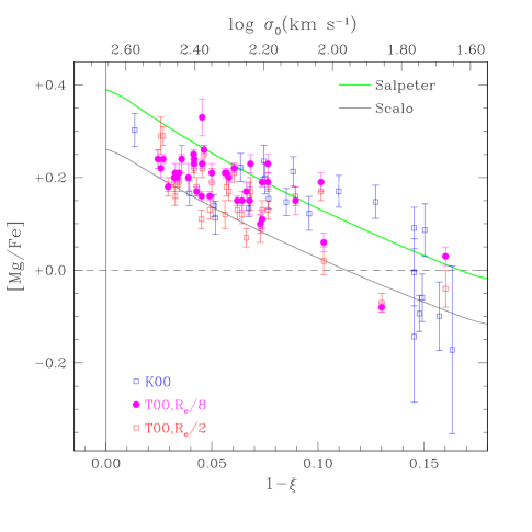
Figure 2: Contribution from SNIa to chemical enrichment. ($1-\xi$) denotes the fractional contribution to the total supernova rate from SNIa, so that $1-\xi=0$ represents a pure contribution from core-collapse supernovae. The data points are from Trager et al. (2000a; T00), evaluated at $R_{e}/8$ (filled squares) and $R_{e}/2$ (hollow circles), and from Kuntschner (2000; K00). The observed data are plotted against central velocity dispersion (top axis). The model prediction is compatible with the data for a linear correlation between central velocity dispersion and SNIa contribution such as: $(1-\xi)=-0.16\log\sigma_{0}+0.43$. The steeper slope of the Scalo IMF at the bright end implies a lower contribution from high mass stars ($M\lower 2.15277pt\hbox{$\;\buildrel>\over{\sim}\;$}20M_{\odot}$), which results in a lower enhancement.

4 Abundance gradients

Observations of colours (Franx et al 1989; Peletier et al. 1990; Jørgensen et al. 1995) and line indices (González 1993; Davies et al. 1993; Peletier et al. 1999) in elliptical galaxies show radial gradients, being redder and richer in metals at their centres. The observed spectral indices display a metallicity gradient of $\Delta[$Fe/H$]/\Delta\log R=-0.2\pm 0.1$ (Davies et al. 1993), consistent with the observed colour gradients. A metallicity gradient can be directly linked to the standard picture of galaxy formation by the dissipative collapse of a gas cloud. Carlberg (1984) analyzed such models with an N-body code, and predicted abundance gradients around $-0.5$ in massive galaxies, flattening towards zero slope in lower mass galaxies. Recent merging events in massive early-type galaxies will dilute any radial signature from an earlier monolithic collapse process, thereby flattening the slope (White 1980; Mihos & Hernquist 1994). Hence, abundance gradients allow us to quantify the degree to which hierarchical clustering has contributed to the formation of galaxies.

We assume a simple model with spherical symmetry and a radially-dependent star formation efficiency. The standard model of star formation assumes a power-law dependence between the star formation rate ($\psi$) and the gas density ($\rho_{g}$; Schmidt 1963), namely:

$$\psi(t)=C_{\rm eff}\rho_{g}^{n}(t)\propto\exp(-t/t_{\rm SF}),$$ (6)

where the constant of proportionality ($C_{\rm eff}$) is the star formation efficiency, and the exponential function is the solution for a linear Schmidt law ($n=1$), in which the star formation timescale $t_{\rm SF}$ can be written as a function of the efficiency timescale ($\tau_{\rm eff}\propto 1/C_{\rm eff}$) and the gas infall timescale ($\tau_{f}$) as:

$$\frac{1}{t_{\rm SF}}=\left(\frac{1}{\tau_{\rm eff}}+\frac{1}{\tau_{f}}\right).$$ (7)

Star formation is known to take place in clouds of molecular hydrogen. Cloud-cloud collisions contribute to the collapse, cooling and subsequent formation of stars. In this simple scenario, we would expect the star formation efficiency to be proportional to the frequency of cloud-cloud collisions, which should scale with the number density of clouds. Hence, the gas density profile traces the star formation efficiency, so that at the centre the star formation timescale should be shorter than in the outer regions. In this scenario $t_{\rm SF}$ is a monotonically increasing function with radius.

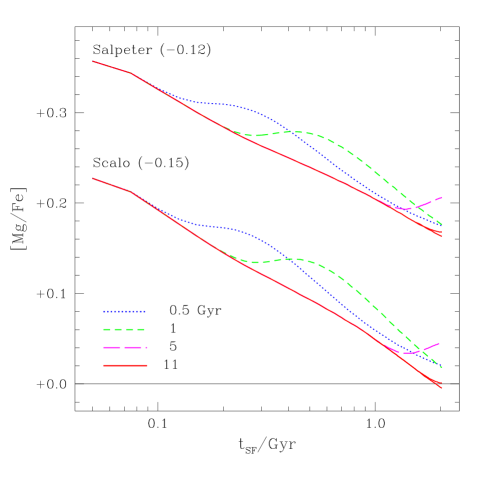
Figure 3: [Mg/Fe] profile as a function of the star formation timescale ($t_{SF}$) which parametrizes the generic star formation history used in this paper. Several curves are given for different ages of the galaxy: 0.5, 1, 5 and 11 Gyr. The numbers in parenthesis give the slope of the profile ($\Delta[$Mg/Fe$]/\Delta\log t_{\rm SF}$) for an age of 11 Gyr.

We assume a generic star formation history described by a gaussian function with a width given by the star formation timescale ($t_{\rm SF}$), which is left as a free parameter. The peak occurs at a time $2\times t_{\rm SF}$ and we assume an age of the Universe of 12 Gyr. Figure 3 shows the predicted relative abundances of this simple model as a function of $t_{\rm SF}$ for both IMFs described above and for a set of ages: 0.5, 1, 5 and 11 Gyr. The number in parenthesis gives the slope of the gradient for both IMFs. It is beyond the scope of this paper to infer a proper functional dependence of the star formation timescale with radius. Hence, we will just assume a generic power-law dependence:

$$t_{\rm SF}\propto r^{\beta}.$$ (8)

We find that the predicted abundance radial gradient for old stellar ages is $\Delta$[Mg/Fe]$/\Delta r\sim-0.15\beta$. In order to compare the model and the observations, we project the 3D radial coordinate ($r$) on to a 2D radius ($R$) using a generic luminosity profile:

$$L(<r)\propto r^{\gamma}\rightarrow L(r)\propto r^{\gamma-3}.$$ (9)

By projecting the volume distribution on to a surface, we can compare the observed slope $a\equiv\Delta$ [Mg/Fe]$/\Delta\log R$ with the model prediction:

$$a=\gamma-2-0.15\beta.$$ (10)

Using the deprojected function presented in Hernquist (1990), which gives a 2D de Vaucouleurs profile, we can choose $\gamma=2$. This value also matches a NFW profile (Navarro, Frenk & White 1997) for radii shorter than the core radius. In this case, the slope of the correlation between radius and star formation timescale can be written:

$$\beta({\rm fixed}\ \gamma)=-\frac{a}{0.15}.$$ (11)

On the other hand, we can fix $\beta$ much in the same way as most semi-analytic modellers do (e.g. Baugh et al. 1998; Kauffmann, White & Guiderdoni 1993) so that the star formation efficiency ($1/t_{\rm SF}$) scales with the dynamical timescale $\sqrt{r^{3}/GM(<r)}$. If we impose a mass-to-light ratio that does not change with radial distance — to be expected in galaxies formed in short duration bursts — we can use equation (9) to write $M(<r)\propto r^{\gamma}$, which implies:

$$\beta=\frac{3-\gamma}{2},$$ (12)

and in turn implies:

$$\gamma=\frac{a+2.225}{1.075}.$$ (13)

Our model assumes that the gradient of the abundance ratios is caused by a formation scenario with different burst lifetimes, which depend on the distance to the centre. One could argue that a large spread of efficiencies in different regions of elliptical galaxies would result in a rather large age spread. However, the age-sensitive Balmer absoption index $H\beta$ does not show any correlation with radial distance (Davies et al. 1993). This implies elliptical galaxies do not have a wide age spread in their stellar populations. Figure 4 shows that even though we consider a large range of star formation timescales, our model is in agreement with the data. We plot in this figure the mass-weighted age of the stellar component as a function of galaxy age for three different star formation timescales. The inset gives the predicted absorption in $H\beta$ as a function of stellar age for simple stellar populations with three different metallicities from the latest population synthesis models of Bruzual & Charlot (in preparation). One can see that after $3-4$ Gyr, it is virtually impossible to determine the stellar ages. This is the age shown as a dashed horizontal line in the figure, which implies that for galaxy ages of 8 Gyr, we can explore a range of star formation timescales up to $t_{\rm SF}\sim 2$ Gyr and still reproduce the observed lack of correlation between radius and Balmer index.

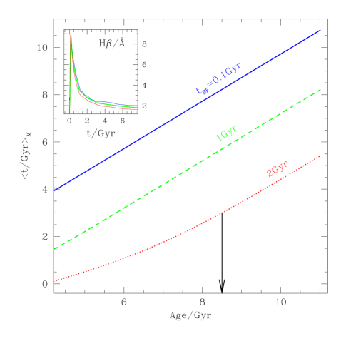
Figure 4: Mass-weighted age of the stellar component as a function of galaxy age for our generic star formation history. The inset shows the predicted equivalent width of $H\beta$ for several metallicities (from the top $Z/Z_{\odot}=\{0.5$,$1$, and $2\}$) using the latest population synthesis models of Bruzual & Charlot (in preparation). Mass-averaged ages older than $\langle t\rangle_{M}\lower 2.15277pt\hbox{$\;\buildrel>\over{\sim}\;$}3$ Gyr (arrow) cannot be discriminated using Balmer indices.

5 Discussion

Our model links the abundance ratios to the star formation timescale, which cannot be directly observed. Instead, the data available give radial gradients. A simple power law, as described in equation (8), can be used in order to throw light on the possible correlation between the infall rate or the star formation efficiency and the dynamical properties of the galaxy. Figure 5 compares the observed radial gradients with the predicted ones, as a function of [Mg/Fe]. The hollow squares represent the data from Trager et al. (2000a), measured at two projected radial positions: $R_{e}/8$ and $R_{e}/2$, which enables us to determine a gradient. A clear trend is seen towards positive gradients in more [Mg/Fe]-enhanced (i.e. more massive) galaxies. The other data points come from the compilation of Kobayashi & Arimoto (1999) from which we selected the work of González (1993, GON); Davies et al. (1993, DSP), and Carollo et al. (1993, CDB) estimated by the authors of the compilation to have the most reliable data. There is a very large scatter in this compilation, with a wide range of slopes, both negative and positive. In agreement with the data from Trager et al. (2000a), a correlation can be seen so that galaxies with positive slopes tend to have the largest super-solar abundances, which correspond to the most massive galaxies as seen in figure 2. The solid line gives a least-squares fit to the data from Trager et al. (2000a). The dashed line also shows a similar trend in the compilation of Kobayashi & Arimoto (1999). Estimating abundance ratios from line indices is still a very delicate issue especially because of the difficulty in finding a suitable set of stars for calibration. Hence, a theoretical approach is called for, using the computations of Tripicco & Bell (1995), who recomputed all of the Lick/IDS spectral indices from a grid of theoretical spectra and atmospheres with varying abundance ratios. The response functions to nonsolar ratios is used to correct the standard population synthesis models of Worthey (1994), calibrated for solar abundance ratios. The uncertainties in such translation frmo abundances to line indices is discussed in Trager et al. (2000a), and an error bar including these uncertainties is shown in figure 5.

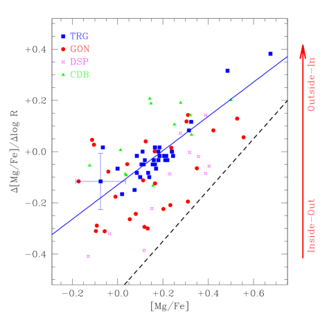
Figure 5: Observed abundance gradients estimated from the measurements of Trager et al. (2000a; TRG; hollow squares) at $R_{e}/8$ and $R_{e}/2$. A typical error bar is shown for illustration. The solid line is a linear squares fit to this data. A rough estimate of [Mg/Fe] gradients from Kobayashi & Arimoto (1999) is also shown. The data points from this compilation correspond to the sample of González (1993, GON); Davies et al. (1993, DSP); and Carollo et al. (1993, CDB). The trend clearly seen in the data from Trager et al. (2000a) as well as hinted at by the void in the lower right corner of the data from Kobayashi & Arimoto (1999), and illustrated by the dashed line, can be interpreted as a hint towards a correlation between galaxy mass (which scales with [Mg/Fe]) and the lower limit of the gradient.

A negative gradient implies an inside-out formation process, which is suggestive of a monolithic collapse scenario, with gas falling towards the centres of dark matter halos, with a gas density profile that decreases outwards and a temperature that decreases inwards, thereby generating a process of star formation that starts at the centre and spreads outwards. On the other hand, recent TreeSPH numerical simulations of galaxy formation (Sommer-Larsen, Gotz & Portinari 2002) find early-type galaxies (both ellipticals and lenticulars) in which star formation proceeds in the opposite way, namely outside-in, mainly triggered by merging. Furthermore, recent observations of field spheroidals in the Hubble Deep Field (Menanteau et al. 2001) show blue cores, result which is currently interpreted as secondary bursts of star formation, but which could be an indication of an outside-in formation process, which implies a positive gradient.

In the light of these data, we infer a varying correlation between the star formation timescale ($t_{\rm SF}$) and galaxy radius. A simple approach, fixing $\gamma$ as in equation (11) gives a slope for this correlation in the range $-1.3<\beta<2$. A better approximation, relating $\beta$ and $\gamma$ through the dynamical timescale, assuming a fixed mass-to-light ratio (12) gives $0.4<\beta<0.6$ with a mass or luminosity profile slope of $1.8<\gamma<2.2$. The higher values of $\gamma$ correspond to positive gradients in the abundance ratio.

The scatter is rather large, and it can only imply a very weak correlation between $\beta$ or $\gamma$ and some dynamical parameter such as central velocity dispersion or mass. This scatter gives another hint of merging as the major mechanism in the assembly process of early-type systems. In a purely monolithic collapse scenario, one would expect a well-defined correlation between the dynamical timescale and the star formation timescale, in such a way that most of the early star formation would occur at the centre. The void in the lower right corner of figure 5 (illustrated by the thick dashed line) shows that we can infer a correlation between [Mg/Fe] (or galaxy mass as shown in Figure 2) and a lower limit to the gradient. This can be interpreted as monolithic collapse being possible only in low mass systems. Higher mass galaxies must be assembled through merging. We emphasize here that the inside-out versus outside-in classification may be an oversimplification. Depending on the simple model we choose — i.e. fixed luminosity profile, as in (11), or correlating $\beta$ with the dynamical timescale, as in (12), massive galaxies give respectively real outside-in star formation ($\beta<0$) or a shallower slope for the correlation between star formation timescale and radius. In either case, the correlation suggested by the dashed line in figure 5 hints at more star formation in the outskirts of massive galaxies compared to low mass systems during the major stage of star formation.

It is worth mentioning that the slope of the abundance ratios is a more robust estimator than the absolute abundance. The latter is strongly dependent on the amount of gas ejected in outflows, which is an important mechanism in early-type galaxies as hinted at by the mass-metallicity relation (Arimoto & Yoshii 1987; Ferreras & Silk 2001), whereas the slope would depend on the scaling of the outflows with radial distance, which should be similar to the scaling of the star formation efficiency and infall timescale, thereby reducing the effect of outflows on the slope.

The radial gradients in abundance ratios represent an alternative way of studying the universality of the IMF, compared to analyses of the metallicities of local stars or the intracluster medium (Wyse 1997). Figure 3 shows that a non-universal IMF would translate into a slope change of the abundance ratio [Mg/Fe]. For instance, if we expect a top-heavy IMF in environments with a high star formation rate (i.e. with a short $t_{\rm SF}$) then the correlation between [Mg/Fe] and star formation timescale should be steeper. However, this calls for a more detailed model which is beyond the scope of this paper. We have also neglected the effect of early galactic winds which could eject $\alpha$-enhanced material out of the galaxy. A correlation of these winds with the local escape velocity could explain the observed radial gradient of Mg abundance in ellipticals (Martinelli, Matteucci & Colafrancesco 1998).

The model presented here relies on the fact that we understand the mechanisms that trigger SNIa and we are able to predict their rates or at least their ratio with respect to SNII. Short bursts of star formation imply that most of the contamination from SNIa will go to the ISM and not so much to the stellar component. Hence, we expect gas in ellipticals to have solar abundance ratios. There has been a long controversy over this point. The study of ASCA observations of a few clusters hinted at a significant SNIa contamination of the gas in rich clusters (Ishimaru & Arimoto 1997). However, Gibson et al. (1997) showed that a different calibration could invalidate this hypothesis. Arimoto et al. (1997) even raised the doubt of whether abundance estimates using the standard iron L-line complex in X-rays is giving wrong metallicities. The latest analysis of six early-type galaxies in Virgo using ROSAT and ASCA observations (Finoguenov & Jones 2000) seem to agree with a high iron content, i.e. an important contribution from SNIa to the enrichment of the ISM in elliptical galaxies.

In this paper, we conclude that a simple treatment of the abundance ratios allows us to infer the star formation history and its connection to the dynamical formation history. The data seems to rule out a monolithic or secular formation scenario for the stellar component of massive ellipticals. On the other hand, the large scatter in the slope of the radial dependence of [Mg/Fe] in low-mass galaxies implies both a merging and a monolithic “mechanism” should be invoked for these systems. A combined analysis of abundance ratios both in the stellar populations and in the interstellar medium will enable us to explore the connection between these two histories, and to quantify the importance of merging events both in the star formation and dynamical histories of early-type galaxies.

References

- [1] Arimoto, N. & Yoshii, 1987, A& A, 173, 23
- [2] Arimoto, N., Matsushita, K., Ishimaru, Y., Ohashi, T. & Renzini, A. 1997, ApJ, 477, 128
- [3] Baugh, C. M., Cole, S., Frenk, C. S. & Lacey, C. G. 1998, ApJ, 498, 504
- [4] Blagaglia, A., Greggio, L., Renzini, A. & d’Odorico, S. 1990, ApJ, 365, L13
- [5] Cappellaro, E., Turatto, M, Tsvetkov, D.-Yu., Bartunov, O. S., Pollas, C., Evans, R. & Hamuy, M. 1997, A&A, 322, 431
- [6] Carlberg, R. G. 1984, ApJ, 286, 403
- [7] Carollo, C . M., Danzinger, I. J. & Buson, L. 1993, MNRAS, 265, 553
- [8] Davies, R. L., Sadler, E. M. & Peletier, R. F. 1993, MNRAS, 262, 650
- [9] Ferreras, I. & Silk, J. 2001, ApJ, 557, 165
- [10] Finoguenov, A. & Jones, C. 2000, ApJ, 539, 603
- [11] Fisher, D., Franx, M. & Illingworth, G. 1996, ApJ, 459, 110
- [12] Franx, M., Illingworth, G., Heckman, T. 1989, AJ, 98, 538
- [13] Gibson, B. K., Loewenstein, M. & Mushotzky, R. F. 1997, MNRAS, 290, 623
- [14] González, J. J. 1993, Ph.D. thesis, Univ. California
- [15] Gratton, R. G., Carretta, E., Matteucci, F. & Sneden, C. 2000, A& A, 358, 671
- [16] Greggio, L. & Renzini, A. 1983, A&A, 118, 217
- [17] Heger, A. & Woosley, S. E. 2002, ApJ, 567, 532
- [18] Hernquist, L. 1990, ApJ, 356, 359
- [19] Iben, I., Jr. & Tutukov, A. V. 1984, ApJS, 54, 335
- [20] Ishimaru, Y., & Arimoto, N. 1997, PASJ, 49, 1
- [21] Jørgensen, I., Franx, M. & Kjægaard, P. 1995, MNRAS, 273, 1097
- [22] Kauffmann, G., White, S. D. M. & Guiderdoni, B. 1993, MNRAS, 264, 201
- [23] Kobayashi, C. & Arimoto, N. 1999, ApJ, 527, 573
- [24] Koester, D. et al. 2001, A&A, 378, 556
- [25] Kuntschner, H. 2000, MNRAS, 315, 184
- [26] Marigo, P., Bressan, A. & Chiosi, C. 1996, A&A, 313, 545
- [27] Martinelli, A., Matteucci, F. & Colafrancesco, S. 1998, MNRAS, 298, 42
- [28] Matteucci, F. & Greggio, L. 1986, A&A, 154, 279
- [29] Matteucci, F. 1994, A& A, 288, 57
- [30] Matteucci, F. & Recchi, S. 2001, ApJ, 558, 351
- [31] Menanteau, F., Abraham, R. G. & Ellis, R. S. 2001, MNRAS, 322, 1
- [32] Mihos, J. C. & Hernquist, L. 1994, ApJ, 427, 112
- [33] Navarro, J. F., Frenk, C. S. & White, S. D. M. 1997, ApJ, 490, 493
- [34] Nomoto, K., Iwamoto, K. & Kishimoto, N. 1997 Science, 276, 1378
- [35] Pancino, E., Pasquini, L., Hill, V., Ferraro, F. R. & Bellazzini, M. 2002, ApJ, 568, L101
- [36] Peletier, R. F. 1989, Ph.D. thesis, Univ. Groningen
- [37] Peletier, R. F., Davies, R. L., Illingworth, G. D., Davis, L. E. & Cawson, M. 1990, AJ, 100, 1091
- [38] Peletier, R. F., Vazdekis, A., Arribas, S., del Burgo, C., García-Lorenzo, B., Gutiérrez, C., Mediavilla, E. & Prada, F. 1999, MNRAS, 310, 863
- [39] Perlmutter, S. et al. 1999, ApJ, 517, 565
- [40] Phillips, M. M. 1993, ApJ, 413, L75
- [41] Riess, A. G. et al. 1998, AJ, 116, 1009
- [42] Salpeter, E. E. 1955, ApJ, 121, 161
- [43] Scalo, J. 1986, Fundam. Cosmic Phys., 11, 1
- [44] Schmidt, M. 1963, ApJ, 137, 758
- [45] Sommer-Larsen, J., Gotz, M. & Portinari, L. 2002, astro-ph/0204366
- [46] Trager, S. C., Faber, S. M., Worthey, G. & González, J. J. 2000a, AJ, 119, 1645
- [47] Trager, S. C., Faber, S. M., Worthey, G. & González, J. J. 2000b, AJ, 120, 165
- [48] Tripicco, M. J. & Bell, R. A. 1995, AJ, 110, 3035
- [49] Thielemann, F., Nomoto, & Yokoi 1986, A&A, 158, 17
- [50] Thielemann, F., Nomoto, & Hashimoto 1996, ApJ, 460, 408
- [51] Tutukov, A. V. & Yungelson, L. R. 1980, in Close binary stars, IAU symp. no. 88, eds. M. J. Plavec, D. M. Popper and R. K. Ulrich, Reidel, Dordrecht, p.15
- [52] Whelan, J. & Iben, I., Jr. 1973, ApJ, 186, 1007
- [53] White, S. D. M. 1980, MNRAS, 191, 1
- [54] Woosley, S. & Weaver, T. 1995, ApJS, 101, 181
- [55] Worthey, G., Faber, S. M. & González, J. J. 1992, ApJ, 398, 69
- [56] Worthey, G. 1994, ApJS, 95, 107
- [57] Wyse, R. F. G. 1997, ApJ, 490, L69