Density profiles of dark matter halos with anisotropic velocity tensors

Abstract

We present density profiles, that are solutions of the spherical Jeans equation, derived under the following two assumptions: (i) the coarse grained phase-density follows a power-law of radius, $\rho/{\sigma}^{3}\propto r^{-\alpha}$, and (ii) the velocity anisotropy parameter is given by the relation $\beta_{a}(r)=\beta_{1}+2\beta_{2}\frac{r/r_{*}}{1+(r/r_{*})^{2}}$ where $\beta_{1}$, $\beta_{2}$ are parameters and $r_{*}$ equals twice the virial radius, $r_{vir}$, of the system. These assumptions are well motivated by the results of N-body simulations. Density profiles have increasing logarithmic slopes $\gamma$, defined by $\gamma=-\frac{\mathrm{d}\ln\rho}{\mathrm{d}\ln r}$. The values of $\gamma$ at $r=10^{-2.5}r_{vir}$, a distance where the systems could be resolved by large N-body simulations, lie in the range $1.-1.6$. These inner values of $\gamma$ increase for increasing $\beta_{1}$ and for increasing concentration of the system. On the other hand, slopes at $r=r_{vir}$ lie in the range $2.42-3.82$. A model density profile that fits well the results at radial distances between $10^{-3}r_{vir}$ and $r_{vir}$ and connects kinematic and structural characteristics of spherical systems is described.

1 Introduction

Density profiles of galactic halos are well fitted by two-power law models. Numerical studies (Quinn et al. [1986]; Frenk et al. [1988]; Dubinski & Garlberg [1991]; Crone et al. [1994]; Navarro et al. [1997], NFW; Cole & Lacey [1996]; Huss et al. [1999]; Fukushige & Makino [1997]; Moore et al. [1998], MGQSL; Jing & Suto [2000], JS) showed that the profile of relaxed halos steepens monotonically with radius. The logarithmic slope $\gamma=-\frac{\mathrm{d}\ln\rho}{\mathrm{d}\ln r}$ is less than 2 near the center and larger than 2 near the virial radius of the system. The value of $\gamma$ near the center of the halo is not yet known. Navarro et al. [1997] claimed $\gamma=1$ while Kravtsov et al. [1998] initially claimed $\gamma\sim 0.7$ but in their revised conclusions (Klypin et al. [2001]) they argue that the inner slope varies from 1 to 1.5. Moore et al. [1998] found a slope $\gamma=1.5$ at the inner regions of their N-body systems.

N-body simulations give also valuable information about the kinematic state of the relaxed structures. Taylor & Navarro [2001], (TN) showed that in a variety of cosmologies the velocity dispersion $\sigma^{2}$ and the density $\rho$ at distance $r$ are connected by a scale free relation $\rho/\sigma^{3}\propto r^{-\alpha}$ with $\alpha=1.875$. They also examined density profiles that resulted from solving the spherical Jeans equation under the above condition assuming an isotropic velocity distribution. Final structures of N-body simulations are radially anisotropic. The radial anisotropy increases outwards taking its maximum value (that is in the range $0.3-0.8$) at about twice the virial radius of the the system. This behavior seems to be universal (Cole & Lacey [1996], Colin et al. [2000], Carlberg et al. [1997]).

In this paper we present solutions of spherical Jeans equation using the above scale free relation given in TN and a model for the velocity anisotropy parameter, in order to construct density profiles for radially anisotropic models. The method for the solution of Jeans equation in described in Sect. 2 and the results are presented in Sect. 3. The conclusions are discussed in Sect. 4.

2 The solution of Jeans equation

Under the assumption of spherical symmetry and no rotation the Jeans equation is:

$$\frac{1}{\rho(r)}\frac{\mathrm{d}}{\mathrm{d}r}(\rho(r){\sigma}_{r}^{2}(r))+\frac{2\beta_{a}(r){\sigma}_{r}^{2}(r)}{r}=-\frac{\mathrm{d}\Phi(r)}{\mathrm{d}r}=-\frac{GM(r)}{r^{2}},\\$$ (1)

where $\beta_{a}$ is the velocity anisotropy parameter given by the relation $\beta_{a}\equiv 1-\frac{{\sigma}^{2}_{t}(r)}{2{\sigma}_{r}^{2}(r)}$ (where ${\sigma}^{2}_{t}$ and ${\sigma}^{2}_{r}$ are the tangential and the radial dispersion of velocities respectively) and $\Phi$ is the potential. Multiplying both sides of (1) with $r^{2}$ and differentiating with respect to $r$ we have

$$\frac{\mathrm{d}}{\mathrm{d}r}\left[{\frac{r^{2}}{\rho(r)}\frac{\mathrm{d}}{\mathrm{d}r}(\rho(r){\sigma}^{2}_{r}(r))+2r\beta_{a}(r){\sigma}^{2}_{r}(r)}\right]=-4\pi G\rho(r)r^{2}.$$ (2)

Under the assumption

$${\rho(r)}/{\sigma}^{3}(r)=(\rho(r_{0})/{\sigma}^{3}(r_{0}))(r/{r_{0}})^{-\alpha},$$ (3)

and after setting $\rho_{0}\equiv\rho(r_{0}),\sigma_{0}\equiv\sigma(r_{0}),x\equiv\ln(r/r_{0})$ and $y\equiv\ln(\rho/{\rho}_{0})$ Jeans equation is written in the form of the following set of differential equations:

$$y^{\prime}_{2}(x)=-ke^{3x+y_{1}(x)},$$ (4)

with $y_{1}(x)\equiv y(x)$ and

$$y^{\prime}_{1}(x)=\frac{3}{5}\left[[3-2\beta_{a}(x)]y_{2}(x)e^{-(\frac{2\alpha+3}{3}x+\frac{2y_{1}}{3})}-\frac{2\alpha}{3}-2\beta_{a}(x)-2\frac{\mathrm{d}\beta_{a}(x)}{\mathrm{d}x}[3-2\beta_{a}(x)]^{-1}\right],\\$$ (5)

where $k\equiv\frac{4\pi G\rho_{0}r^{2}_{0}}{\sigma^{2}_{0}}$. Note that $\sigma$ in (3) is the total dispersion of velocities.
TN showed that the isotropic case ($\beta_{a}\equiv 0$) admits a solution $y_{1}(x)=-\beta x$, (power law in $r-\rho$ space), with $\beta=6-2\alpha$ and $k=2(\beta-1)(3-\beta)/3$. Additionally they used $\alpha=1.875$, a value resulting from the final structures of N-body simulations, to show that for values of $k$ larger than the one that corresponds to the above power-law solution, the density profiles become complex and that for values of $k$ larger than a critical value $k_{crit}$, the density profiles become unrealistic since densities are vanished at some finite radius near the center of the system. The density profile that corresponds to $k_{crit}$ scales as $r^{-0.75}$ in the inner region of the system, close to the NFW profile that scales as $r^{-1}$.

Since the anisotropy of velocities is always present in the results of N-body simulations, it should be interesting to study its effects on the solutions of Jeans equation. N-body simulations for a variety of cosmologies show an almost universal variation of $\beta_{a}$. Starting from the center of the system, $\beta_{a}$ increases outwards taking its maximum radius at about twice the virial radius $r_{vir}$ of the system. The maximum value is in the range 0.3-0.8 (Cole & Lacey [1996], Colin et al. [2000], Carlberg et al. [1997]). Thus we model $\beta_{a}$ as

$$\beta_{a}(r)=\beta_{1}+2\beta_{2}\frac{r/r_{*}}{1+(r/r_{*})^{2}}$$ (6)

where $r$ is the radial distance. The maximum value of $\beta_{a}$ is $\beta_{max}=\beta_{1}+\beta_{2}$ and it is achieved at $r=r_{*}=2r_{vir}$. The initial conditions required for the solution of the above set of differential equations are set in a similar way as in TN: At a radius $r_{0}=1$ we assume a density $\rho_{0}=1$ and $\gamma(r_{0}=1)=2.25$. Thus we take $y_{1}(0)=0$ and $y^{\prime}_{1}(0)=-2.25$. Furthermore, the value of $y_{2}(0)$ is calculated by solving equation (5) for $y_{2}$ leading to the relation:

$$y_{2}(0)=\frac{1}{3-\beta_{a}(0)}\left[\frac{2\alpha}{3}-\frac{5\beta}{3}+2\beta^{\prime}_{a}(0)[3-2\beta_{a}(0)]^{-1}+2\beta_{a}(0)\right]$$ (7)

Obviously $y^{\prime}_{2}(0)=-k$. Then we integrate inwards and outwards to calculate density profiles.

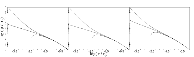
Figure 1: Density profiles derived from the solution of Jeans equation for fixed values of $\beta_{1},\beta_{2}$ and $c$ and varying $k$. For values of $k$ larger than a $k_{crit}$ densities vanish at a finite radius near the center while for $k<k_{crit}$ the slopes increase inwards.

3 Density profiles

The calculation of density profiles is organized as follows: For given values of $r_{vir},\beta_{1},\beta_{2}$ we find the solution of Jeans equation for the maximum value of $k$, named $k_{crit}$, for which the density is a decreasing function of the radial distance. An example of the behavior of the solutions in the inner region of the system is presented in Fig. 1. The curves shown in the left panel are solutions for $\beta_{1}=0,\beta_{2}=0.8$ and $r_{vir}/r_{0}=10$. The upper line corresponds to $k=0.84$, the middle one is the critical solution corresponding to $k=k_{crit}=0.85114$ and the lower one corresponds to $k=0.86$. The middle panel shows solutions for $r_{vir}/r_{0}=5,\beta_{1}=0$ and $\beta_{2}=0.3$. The upper line corresponds to $k=0.85$, the middle one is the critical solution corresponding to $k=0.86146$ and the lower one to $k=0.87$. The right panel contains the solutions for $\beta_{1}=0.15,\beta_{2}=0.35$ and $r_{vir}/r_{0}=10$. The critical solution (middle curve) is obtained for $k=k_{crit}=0.80031$ while the upper and lower curves are solutions for $k=0.79$ and $k=0.81$ respectively. It is shown in this Fig. that for values of $k$ smaller than $k_{crit}$ the slope of the density profile changes significantly at the inner region of the system where it becomes very steep, while for $k>k_{crit}$ density profile becomes unrealistic since it vanishes at a finite distance from the center. Although there is no obvious physical reason to exclude solutions with $k<k_{crit}$ we note that such a behavior of the density profile has not been reported elsewhere and so we restrict ourselves to the study of critical solutions alone.

We studied $21$ different cases. The values of the parameters for every case as well as the resulting values of $k_{crit}$ are given in the Table 1. A convenient concentration parameter $c$ is defined by the relation $c\equiv r_{vir}/r_{0}$, that is the ratio of the virial radius to the radius where the logarithmic slope of the density profile equals to $2.25$.

TN illustrated that the critical solution ($k=k_{crit}$) for the isotropic velocity case yielded a phase-space distribution function ($\mathrm{d}M/\mathrm{d}log({\sigma}^{3}/\rho)$) that was the most peaked, or ’maximally mixed’ (excluding cases that produced hollow-core density profiles). We show that the same holds in anisotropic cases. The left panel of Fig. 2 presents the phase space distribution function for the case with $c=10$, $b_{1}=0$ and $b_{2}=0.8$. The most peaked curve corresponds to $k=k_{crit}=0.85114$ the middle one to $k=0.84$ and the lower one to $k=0.82$. The right panel presents the case with $c=10$, $b_{1}=0.15$ and $b_{2}=0.35$. The most peaked curve of the this panel corresponds to $k=k_{crit}=0.80031$, the middle one to $k=0.78$, while the lower one to $k=0.76$.

Table 1: The parameters and the resulting values of $k_{crit}$ for Cases 1-21

Case No	$c$	$\beta_{1}$	$\beta_{2}$	$k_{crit}$	Case No	$c$	$\beta_{1}$	$\beta_{2}$	$k_{crit}$
Case 1	10.	0.00	0.80	0.85114	Case 10	10.	0.15	0.65	0.78410
Case 2	5.	0.00	0.80	0.80947	Case 11	5.	0.15	0.65	0.74800
Case 3	2.5	0.00	0.80	0.72034	Case 12	2.5	0.15	0.65	0.67110
Case 4	10.	0.00	0.50	0.86638	Case 13	10.	0.15	0.35	0.80031
Case 5	5.	0.00	0.50	0.84107	Case 14	5.	0.15	0.35	0.78150
Case 6	2.5	0.00	0.50	0.78992	Case 15	2.5	0.15	0.35	0.74380
Case 7	10.	0.00	0.30	0.87642	Case 16	10.	0.15	0.15	0.81100
Case 8	5.	0.00	0.30	0.86146	Case 17	5.	0.15	0.15	0.80310
Case 9	2.5	0.00	0.30	0.83184	Case 18	2.5	0.15	0.15	0.78750
					Case 19	10.	0.30	0.50	0.71704
					Case 20	5.	0.30	0.50	0.68700
					Case 21	2.5	0.30	0.50	0.62330

The resulting density profiles are fitted by curves of the form

$$\rho_{fit}(r)=\frac{\rho_{c}}{(\frac{r}{r_{s}})^{\lambda}{(1+(\frac{r}{r_{s}})^{\mu})}^{\nu}}.\\$$ (8)

Models with density cusps that have been proposed in the literature belong to the above class of density profiles. For $\lambda=1,\mu=1$ and $\nu=2$ Eq.(8) corresponds to the NFW model. The model proposed by Hernquist ([1990]) has $\lambda=1,\mu=1$ and $\nu=3$. MGQSL proposed the model with $\lambda=1.5,\mu=1.5$ and $\nu=1$ while JS estimated $\lambda=1.5,\mu=1$ and $\nu=1.5$ for galaxy-size halos. The fitting parameters $\rho_{c}$, $r_{s}$, $\lambda$, $\mu$ and $\nu$ of Eq.(8) are calculated finding the minimum of the sum

$$S=\sum_{i=1}^{NP}\left[\log\rho_{J}(r_{i})-\log\rho_{fit}(r_{i})\right]^{2}$$ (9)

where $\rho_{J}$ is the density profile predicted by the above described solution of Jeans equation. The minimum of $S$ is found using the unconstrained minimizing subroutine ZXMWD of IMSL mathematical library.

Figure 2: The phase-space distribution function for anisotropic cases. The most peaked curves correspond to the critical values of $k$ for every case.The left panel presents systems with $c=10$ $b_{1}=0$ and $b_{2}=0.8$ while the right one shows systems with $c=10$ $b_{1}=0.15$ and $b_{2}=0.35$. The systems of every panel have the same mass and energy.

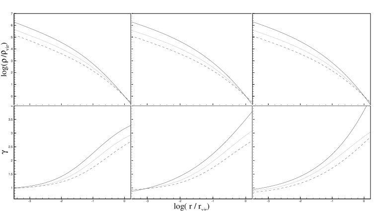
Figure 3: Density profiles and their logaritmic slopes for Cases 1 to 9. First column: Cases 1, 2 and 3 (solid, dotted and dashed line respectively). Second column: as in the first column but for Cases 4, 5, 6. Third column: as in the first column but for Cases 7, 8, 9.

We used values of the density at radial distances in the range $10^{-3.5}r_{vir}$ to $1.5r_{vir}$. The logarithmic slope of the density profile at $r\rightarrow 0$ is given by the value of $\lambda$. For the first nine cases, that are all isotropic at the center ($\beta_{1}=0$), values of $\lambda$ that result from the above fitting are in the range $0.71-0.98$. For the next nine cases (Cases 10 to 18) that have $\beta_{1}=0.15$ the values of $\lambda$ are in the range $0.82-1.02$ while for the last three cases (Cases 19, 20 and 21), that are highly anisotropic at the center ($\beta_{1}=0.3$) the values of $\lambda$ are in the range $1.06-1.22$. We also note that in all cases the values of $\mu$ are in the range $0.32-0.61$ in contrast to all the proposed models that give $\mu\geq 1$.

The quality of fit is excellent and it allows a very good estimation of the logarithmic slope of the density profile all the way from very small to vary large radii through the relation:

$$\gamma=-\frac{\mathrm{d}{\ln(\rho(r))}}{\mathrm{d}\ln r}=\lambda+\mu\nu\frac{(r/r_{s})^{\mu}}{1+(r/r_{s})^{\mu}}$$ (10)

The results for all cases are presented in Fig. 3 and Fig. 4. Figure 3 consists of six panels that show the density profiles as well as the logarithmic slopes of these profiles for the first nine cases. The two figures of the first column correspond to the Cases 1, 2 and 3 (solid, dotted and dashed lines respectively). The second column shows the results for the Cases 4, 5 and 6 respectively while the third one contains the results for Cases 7, 8 and 9. Densities are normalized to the virial density of every case, that is the density of the system at its virial radius, while distances are normalized to the virial radius. In a similar way the rest 12 cases are presented in Fig. 4. The first column shows the Cases 10, 11 and 12 (solid, dotted and dashed line respectively). Cases 13, 14 and 15 are shown in the two figures of the second column. The third column shows the Cases 16, 17 and 18 and the last one corresponds to the three last Cases 19, 20 and 21. In this way every column shows three cases that have the same values of $\beta_{1}$ and $\beta_{2}$ but different values of $c$. Additionally, irrespectively of the column, solid lines correspond to systems with $c=10$, dotted lines to systems with $c=5$ and dashed lines to systems with $c=2.5$

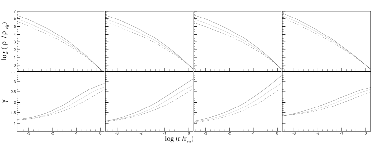
Figure 4: As in Fig.3 but for Cases 10-21.

The results lead to the following conclusions:

1. The slope of the density profile at the central region is closely connected to the amount of the anisotropy of velocities there. It is larger for larger anisotropy. For example at $r=10^{-2.5}r_{vir}$ the first nine Cases 1 to 9 that have $\beta_{1}=0.0$ show central slopes near to unity $[1-1.18]$. Cases 10 to 18 that correspond to $\beta_{1}=0.15$ have slopes in the range $[1.25-1.39]$ and the last three cases, 19, 20 and 21 that have highly anisotropic central regions, ($\beta_{1}=0.3$), have slopes in the range $[1.49-1.61]$.

2. Structures resulting for the same values of $\beta_{1}$ and $\beta_{2}$ show inner slopes that depend on their concentrations. This dependence is not very clear at very small radii, (for example at $r=10^{-3.5}r_{vir})$ but it is obvious at larger radii as those that can be resolved by N-body simulations, $(r\approx 10^{-2.5}r_{vir})$. Thus, if the values of $\beta_{1}$ and $\beta_{2}$ are universal, systems with larger $c$ have larger slopes than those with smaller $c$ at distances that are the same fraction of their virial radii. Note that the results of N-body simulations suggest that $c$ is a decreasing function of the virial mass of the system (NFW, Bullock et al. [2001]). Thus, our results indicate that inner slopes are smaller for systems with larger masses. This dependence is in accordance with the results of N-body simulations. For example JS found that, at $r=0.01r_{vir}$, the slope is $\approx 1.5$ for galaxy-size halos and $\approx 1.1$ for galaxy cluster-size halos respectively. We note at this point that our concentration parameter $c$ is related to the concentration parameter of NFW, $c_{NFW}\equiv r_{vir}/r_{s,NFW}$, by the relation $c_{NFW}=(3/5)c$. The results of N-body simulations indicate that for galaxy-size halos $c_{NFW}\approx 17$ (that corresponds to $c=10$), while for galaxy cluster-size halos $c_{NFW}\approx 7$ that corresponds to $c\approx 4.2$.

3. Slopes at $r=r_{vir}$ show values in the range $2.42-3.82$. For systems with the same values of $\beta_{1}$ and $\beta_{2}$ outer slope is an increasing function of $c$. On the other hand, a comparison between systems with the same values of $c$ and $\beta_{1}$ shows that the ones with smaller values of $\beta_{2}$ have larger outer slopes.

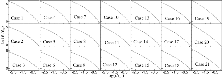
Figure 5: A comparison of all resulting density profiles with our model. Solid lines are the solutions of Jeans equation while the predictions of our fitting models are shown by squares.

We summarize the above results by proposing a fitting formula (FF), that holds for the range $10^{-3}r_{vir}$ to $r_{vir}$ and connects the values of the exponents $\lambda,\mu$ and $\nu$ of Eq. (8) with the values of $\beta_{1}$ and $\beta_{2}$. That is:

$$\lambda=1+2\beta_{1},\mu=0.75-0.3\beta_{1},\nu=\frac{3-2\beta_{1}-\beta_{2}}{\mu}$$ (11)

The two remaining fitting parameters $\rho_{c}$ and $r_{s}$ are found by the minimization procedure described above. The results are shown in Fig. 5. Solid lines are the solutions of Jeans equation while squares are the respective fits given by FF. The fit is more than satisfactory.

Additionally, the resulting concentrations are compared to the input concentrations by the following way: Consider $r_{n}$ the radius where the slope equals to $n$. This $r_{n}$ is related to the fitting parameters by the relation:

$$r_{n}=\left(\frac{n-\lambda}{\lambda+\mu\nu-n}\right)^{\frac{1}{\mu}}r_{s}.$$ (12)

The concentration of the system, resulting from the fitting procedure, is $c_{f}=r_{vir}/r_{2.25}$. The values of $c_{f}$ are close enough to the input values of the concentration $c$. For systems with $c=10$ the values of $c_{f}$ are in the range of $7.8-12.58$, for systems with $c=5$ the values of $c_{f}$ lie in the range $4.28-5.33$, while the density profiles of systems with $c=2.5$ are fitted by density profiles with $c_{f}$ in the range $2.02-2.8$.

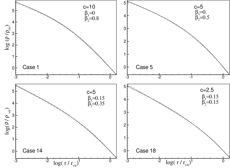
Figure 6: Comparison of resulting density profiles with other models. Solid lines: solutions of Jeans equation, dashed lines: NFW fit (for cases 1 and 5) and MGQSL fit (for cases 14 and 18), circles: FF fit.

In Fig. 6 a detailed comparison between various models is shown. For Cases 1 and 5 the solutions of Jeans equation are shown as solid lines, the results of FF as dotted line and the NFW profile as dashed lines. For cases 14 and 18 solids and dotted lines show the same profiles as in Cases 1 and 5 while dashed lines correspond to the MGQSL profile. It is clear that the NFW profile is an excellent fit for the Case 5 and a very good fit for the Case 1. On the other hand MGQSL is an excellent fit to Case 14 and a good enough fit to Case 18. The FF gives very good fits for all four cases. It is characteristic that analytical models with different values of the parameters $\lambda,\mu$ and $\nu$ can fit equally well the same density profile. This indicates the large degree of degeneracy in these parameters that is already noticed by Klypin et al. [2001]. However a question naturally arises at this point. Can both popular models of NFW and MGQSL fit equally well the same density profile? The answer is no as it can be obtained by looking at Fig.7. Solid lines are the solutions of Jeans equation, dashed lines are the best NFW fit while dotted lines correspond to MGQSL fit. The results of FF are shown as small circles. For the centrally isotropic Case 8 the NFW profile is an excellent fit. For this Case the MGQSL profile does not approximate well the results. On the other hand the results of Case 10, that corresponds to a centrally anisotropic system, are fitted well by the MGQSL profile while the NFW is less steep near the central region and also differs at intermediate distances. The FF is a very satisfactory fit to both cases.

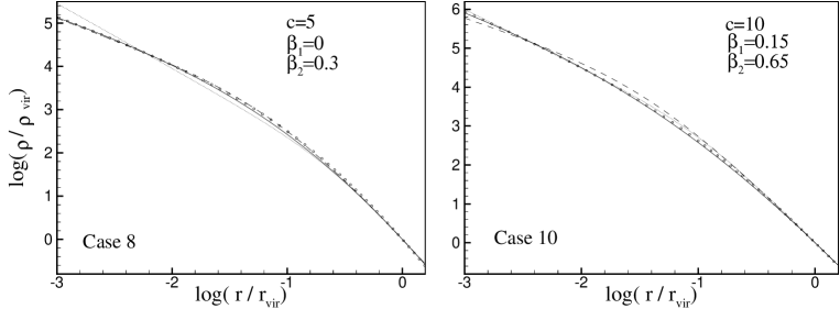
Figure 7: Comparison of resulting density profiles with other models. Solid lines: solutions of Jeans equation, dashed lines: NFW fit, dotted lines: MGQSL fit, circles: FF fit.

4 Discussion

This paper presents density profiles of spherical systems derived by the solution of spherical Jeans equation. These profiles, derived under two assumptions described in previous sections, show a considerable agreement with models proposed in the literature. The results show a number of trends relating kinematic and structural characteristics of the systems. A formula that fits very well the results for $r\geq 10^{-3}r_{vir}$ and connects the values of the anisotropy velocity parameter to the form of the density profile is proposed. If all cases studied above do represent final states of real systems then the idea of a density profile with fixed values of $\lambda,\mu$ and $\nu$ able to fit all halos, by just adjusting the concentration, is not favored. However it should be interesting, large N-body simulations, that are the most powerful methods to deal with the formation of structures, to answer some of the questions that naturally arise by our results. Such questions relate to the validity of our two main assumptions, the universality of the values of $\beta_{1}$ and $\beta_{2}$ as well as the relation between the values of these two parameters and the mass of the system. Answering these questions should reduce the parameter space and help to construct better analytical models so as to improve our understanding about the formation of structures in the universe.

5 Acknowledgements

I would like to thank the referee James Bullock for providing constructive comments on this manuscript and the Empirikion Foundation for its support.

References

- [2001] Bullock, J. S., Kolatt, T. S., Sigad, Y., Somerville, R. S., Kravtsov, A.V., Klypin, A. A., Primack, J. R., Dekel, A., Profiles of dark haloes: evolution, scatter and environment, 2001, MNRAS, 321, 559 (2001MNRAS.321..559B)
- [1997] Carlberg, R. G., Yee, H. K. C., Ellingson,E., The Average Mass and Light Profiles of Galaxy Clusters, 1997, ApJ, 478, 462 (1997ApJ...478..462)
- [1996] Cole, S. & Lacey, C., The structure of dark matter haloes in hierarchical clustering models, 1996, MNRAS, 281, 716 (1996MNRAS.281..716C)
- [2000] Colin, P., Klypin, A. A. & Kravtsov, A. V. Velocity Bias in a Cold Dark Matter Model, 2000, ApJ, 539, 561 (2000ApJ...539..561C)
- [1994] Crone, M. M., Evrard, A. E. & Richstone, D. O., The cosmological dependence of cluster density profiles, 1994, ApJ, 434, 402 (1994ApJ...434..402C)
- [1991] Dubinski, J. & Carlberg, R.G., The structure of cold dark matter halos, 1991, ApJ, 378, 496 (1991ApJ...378..496D)
- [1988] Frenk, C.S, White, S. D. M., Davis, M. & Efstathiou, G., The formation of dark halos in a universe dominated by cold dark matter, 1988, ApJ, 327, 507 (1988ApJ...327..507F)
- [1997] Fukushige, T., & Makino, J., On the Origin of Cusps in Dark Matter Halos, 1997, ApJ, 477, L9 (1997ApJ...477L...9F)
- [1990] Hernquist, L., An analytical model for spherical galaxies and bulges, 1990, ApJ, 356, 359 (1990ApJ...356..359H)
- [1999] Huss, A., Jain B. & Steinmetz, M., The formation and evolution of clusters of galaxies in different cosmogonies, 1999, MNRAS, 308, 1011 (1999MNRAS.308.1011H)
- [2000] Jing, Y. P. & Suto, Y., The Density Profiles of the Dark Matter Halo Are Not Universal, 2000, ApJ, 529, L69 (JS) (2000ApJ...529L..69J)
- [1998] Kravtsov, A. V., Klypin, A. A., Bullock, J. S. & Primack, J. R., The Cores of Dark Matter-dominated Galaxies: Theory versus Observations, 1998, ApJ, 502, 48 (1998ApJ...502...48K)
- [2001] Klypin, A. A., Kravtsov, A. V., Bullock, J. S. & Primack, J. R., Resolving the Structure of Cold Dark Matter Halos, 2001, ApJ, 554, 903 (2001ApJ...554..903K)
- [1998] Moore, B., Governato, F., Quinn, T., Stadel, J. & Lake, G., Resolving the Structure of Cold Dark Matter Halos, 1998, ApJ, 499, L5 (MGQSL) (1998ApJ...499L...5M)
- [1997] Navarro, J. F., Frenk, C. S. & White, S. D. M., A Universal Density Profile from Hierarchical Clustering, 1997, ApJ, 490, 493 (NFW) (1997ApJ...490..493N)
- [2001] Taylor, J. E., Navarro, J. F., The Phase-Space Density Profiles of Cold Dark Matter Halos, 2001 ApJ, 563, 483 (TN) (2001ApJ...563..483T)
- [1986] Quinn, P.J., Salmon, J. K. & Zurek, W. H., Primordial density fluctuations and the structure of galactic haloes, 1986, Nature, 322, 329 (1986Natur.322..329Q)