Thermal Pressures in Neutral Clouds inside the Local Bubble, as Determined from C I Fine-Structure Excitations

Abstract

High-resolution spectra covering the absorption features from interstellar C I were recorded for four early-type stars with spectrographs on the Hubble Space Telescope, in a program to measure the fine-structure excitation of this atom within neutral clouds inside or near the edge of the Local Bubble, a volume of hot ($T\sim 10^{6}\,$K) gas that emits soft x-rays and extends out to about 100 pc away from the Sun. The excited levels of C I are populated by collisions, and the ratio of excited atoms to those in the ground level give a measure of the local thermal pressure. Absorptions from the two lowest levels of C I were detected toward $\alpha$ Del and $\delta$ Cyg, while only marginal indications of excited C I were obtained for $\gamma$ Ori, and $\lambda$ Lup. Along with temperature limits derived by other means, the C I fine-structure populations indicate that for the clouds in front of $\gamma$ Ori, $\delta$ Cyg and $\alpha$ Del, $10^{3}<p/k<10^{4}\,{\rm cm}^{-3}\,$K at about the $\pm 1\sigma$ confidence level in each case. The results for $\lambda$ Lup are not as well constrained, but still consistent with the other three stars. The results indicate that the thermal pressures are below generally accepted estimates $p/k>10^{4}\,{\rm cm}^{-3}\,$K for the Local Bubble, based on the strength of x-ray and EUV emission from the hot gas. This inequality of pressure for these neutral clouds and their surroundings duplicates a condition that exists for the local, partly-ionized cloud that surrounds the Sun. An appendix in the paper describes a direct method for determining and eliminating small spectral artifacts arising from variations of detector sensitivity with position.

1 Introduction

The Sun is immersed in two concentric volumes of interstellar material with very different properties. In the immediate surroundings [out to distances ranging from 0.05 to several pc away (Redfield & Linsky 2000)], the gas is partly ionized, with characteristic properties $0.10<n({\rm H~{}I})<0.24\,{\rm cm}^{-3}$, $0.04<n(e)<0.10\,{\rm cm}^{-3}$ and $T\approx 7500\,$K (Lallement 1998; Puyoo & Ben Jaffel 1998; Ferlet 1999; Gry & Jenkins 2001). This cloud, often called the Local Interstellar Cloud (LIC), is surrounded by a large cavity containing fully-ionized, very hot, low-density material with $n({\rm H}^{+})\approx 0.008\,{\rm cm}^{-3}$ and $T\sim 10^{6}\,$K (Berghöfer et al. 1998; Burrows & Guo 1998) that is prominent in soft x-ray emission (Snowden et al. 1990, 1998). This large volume of hot gas is believed to be the product of probably several supernova explosions (Cox & Reynolds 1987; Breitschwerdt & Schmutzler 1994; Maíz-Apellániz 2001; Smith & Cox 2001) and is known as the Local Bubble (LB). The LB is also conspicuous by showing a general absence of cold, neutral gas up to a well defined boundary (Sfeir et al. 1999; Vergely et al. 2001), as is shown in Figure 1.

A persistent puzzle has been the apparent mismatch in thermal pressures between the two media. Using the parameters stated above, one finds that $1400<p/k<3600\,{\rm cm}^{-3}\,$K for the LIC, which contrasts with an apparent representative value of $16,000\,{\rm cm}^{-3}\,$K for the fully-ionized, hot gas in the LB. The objective of the research presented here is to help answer the question, “What thermal pressures are found for other neutral clouds within the Local Bubble? That is, do they have values similar to the LIC, or are they closer to matching the apparent pressure of the LB?” To gain insights on this question, one can observe stars located behind individual clouds inside the LB and measure their absorption features of C I arising from different fine-structure levels of the ground state. The ratios of populations of these states are governed by an equilibrium between collisional excitations (governed by local densities and temperatures) and spontaneous radiative decays.

Stars suitable for viewing the C I features had to satisfy a number of conditions to yield useful results. Their selection is described in §2; ultimately four such stars were observed in a manner described in §3. The C I absorption features are very weak, and in order to obtain useful measures of their strengths particular care was exercised to remove spurious signals arising from the detector, as outlined in §4.1. (Mathematical details about the correction method are presented separately in the Appendix.) Section 5 describes how the equivalent widths of various absorption features were combined and corrected for saturation (very mild, except for one of the stars). This section also discusses the derivations of fine-structure population ratios, which may be compared to the theoretically expected values for different conditions (§6.1). Before one can derive useful limits for the thermal pressures, the allowable ranges of temperature must be constrained, and different methods of deriving these constraints are discussed in §6.2. Ultimately, the limits for the population ratios and temperatures restrict the possible values for $p/k$ [and local density $n({\rm H})$], as shown for the four cases in the diagrams presented in Fig. 7. Three out of the four stars indicate internal thermal pressures for the foreground clouds that are below the generally accepted value for the LB. Possible explanations for this imbalance, duplicating that seen for LIC, are presented in §7.

2 Selection of Target Stars

Target stars chosen for the survey had to satisfy four fundamental criteria. First, the stars had to be within the Local Bubble or near its edge. Second, they had to have sufficient neutral gas in front so that there was a reasonable expectation of seeing the C I absorption features. Third, the stars had to be bright enough to give a good signal-to-noise ratio in a reasonably short observing time. Finally, the survey avoided stars with projected rotational velocities $v\sin i<50\,{\rm km~{}s}^{-1}$ (Uesugi & Fukuda 1981 – with actual values provided by the VizieR web site at the Strasbourg Data Center), so that stellar features would not cause confusion when the interstellar lines were being identified and measured. To satisfy the first two requirements, the selection included stars less than about 100 pc away that had interstellar D-line absorption features indicating $10^{11}<N$(Na I) $<3\times 10^{11}\,{\rm cm}^{-2}$. A compilation by Welsh et al (1994) was a good source of information about D-line absorption at the time the survey was being planned. Fluxes at 1565 Å listed in the TD-1 Catalogue of Stellar Ultraviolet Fluxes (Thompson et al. 1978) provided a good guide for selecting targets with satisfactory brightness levels.

To increase the chance that the C I features arose from truly intervening material rather than circumstellar disks or shells around the target stars, the survey did not include candidates that had spectral types with an emission-line “e” designation (Hoffleit & Jaschek 1982; Slettebak 1982) or an excess IRAS flux at $12\mu$m relative to the normal expectation. Short-period binaries were also rejected, since they could have interacting gas streams. As a final precaution against skewing the results with cases dominated by gaseous material very near the stars, there was an exclusion of targets that had excess diffuse infrared emission nearby in the sky (Gaustad & Van Buren 1993), signifying the possible presence of dust grains being heated by the star.

Four stars that were ultimately chosen for the survey are listed in Table 1. Their locations with respect to the Local Bubble boundaries mapped by Sfeir et al. (1999) are shown in Figure 1.

Figure 1: Locations of the four program stars listed in Table 1 with respect to the shape of the Local Bubble in the plane of the Galaxy, outlined by contours of increasing Na I D2-line absorption equivalent widths mapped by Sfeir et al (1999). The Galactic center direction is toward the right. To maintain consistency with Sfeir et al’s construction of the contours according to a spherical projection, the distances of the stars from the origin are not foreshortened by $\cos(b)$.

Table 1: Target Stars and Dataset Identifications

Star	HD	$\ell$	$b$	$d$	Spectral	HST Archive
Name	Nr.	(deg)	(deg)	(pc)	Type	Dataset Name
$\gamma$ Ori	35468	196.9	$-16.0$	$75\pm 6$	B2 III	Z3CI0107T
$\lambda$ Lup	133955	326.8	+11.1	$125\pm 11$	B3 V	Z3CI0307T
$\delta$ Cyg	186882	78.7	+10.2	$52\pm 1$	B9.5 IV	Z3CI0407T
$\alpha$ Del	196867	60.3	$-15.3$	$74\pm 4$	B9 IV	O50001010-40

3 Observations

The Goddard High Resolution Spectrograph (GHRS) on HST had a proven capability of achieving large signal-to-noise ratios for bright targets (Cardelli & Ebbets 1994; Cardelli 1995). For this reason, this instrument was considered ideal for the objective of recording the weak C I absorption features. The survey was originally intended to be completed before GHRS was to be replaced by the Space Telescope Imaging Spectrograph (STIS) during the second HST servicing mission, but useful observations of $\alpha$ Del were not accomplished until after STIS was installed.

Observations of $\gamma$ Ori, $\lambda$ Lup and $\delta$ Cyg were carried out with the Ech-A grating on GHRS, with a substep pattern that created 4 spectrum bins per detector diode (STEP-PATT=7) plus a sampling of the background level. The standard option for spectrum shifts (FP-SPLIT mode) allowed for an elimination of the detector’s fixed-pattern noise in the spectrum (§4.1 and Appendix A). The GHRS observations were performed with COSTAR in place to correct for the telescope’s spherical aberration, and the 2″ entrance aperture was used to increase the efficiency. The STIS observations of $\alpha$ Del with the E140H grating had to be done using neutral density filters to prevent the MAMA detector count rate limits from being exceeded. The wavelength resolving powers of the GHRS observations were $\lambda/\Delta\lambda=90,000$ [but with some extended wings in the line-spread function – see Howk, Savage & Fabian (1999)], while that for the STIS spectrum of $\alpha$ Del is 110,000 (Kimble et al. 1998; Leitherer 2001).

The limited wavelength coverage of the GHRS Digicon detector for echelle spectroscopy limited observations to only one multiplet at any particular moment. The multiplet of choice was the one at 1260 Å, since it had well separated lines and was near the peak in the instrument’s sensitivity. However, for late B-type stars ($\delta$ Cyg and $\alpha$ Del), a strong stellar feature seriously depresses the flux level at the position of this multiplet, so other multiplets had to be viewed for these stars. The STIS observation of $\alpha$ Del covered many multiplets, but only the strong ones listed in Table 2 gave useful results. For all stars, the S II triplet with features at 1250.584, 1253.811 and 1259.519 Å was also observed to monitor the presence of a generally undepleted element in its favored stage of ionization in an H I region. The abundance of S II served a useful purpose in constraining the temperature of the gas, as outlined in §6.2.

4 Data Reduction

4.1 Removal of Detector Artifacts

In order to realize the full potential of GHRS in sensing very weak absorption features, it was necessary to remove spurious signal deviations caused by small changes in photocathode sensitivity with position. The intentional displacements in wavelength for different subexposures in the GHRS FP-SPLIT observing routine allowed these variations to be differentiated from real absorption features in the raw spectra. The method used here to derive independently the detector’s fixed-pattern signal and the real spectral signal gave a direct solution and thus differed from the iterative technique described by Ebbets (1992), Cardelli & Ebbets (1994) and Fitzpatrick & Spitzer (1994). Details of this more direct method of solution are given in Appendix A.

It is important to recognize that for any given wavelength offset within the FP-SPLIT procedure, there are two effects that can alter the mapping of photocathode points onto given spectral bins. One of them is a change caused by the Doppler-shift correction for orbital motion (performed internally by GHRS). The extremes of this correction can in principle differ by as much as twice the orbital velocity of approximately $7\,{\rm km~{}s}^{-1}$ times the cosine of the angle of the target with respect HST orbital plane at the time of observation. The other effect, a much smaller one, arises from small changes in the influence of the Earth’s magnetic field on the trajectories of the electrons traveling from the detector’s photocathode to the sensing diodes (Ebbets 1992). Figure 2 illustrates the importance of recognizing these shifts and compensating for them in the analysis that eliminates the fixed-pattern noise. The top panel shows a straight average of the spectra of $\gamma$ Ori (i.e., no attempt to correct for the fixed-pattern noise), after shifts had been implemented to compensate for spectral motions with respect to the diodes. The middle panel shows the outcome for an initial attempt to correct for the fixed-pattern variations by assuming that they remained stationary with respect to the pixel assignments in the accumulated signal transmitted to the ground. Practically no improvement over the simple average is apparent after this correction. However, one may track the movement of the photocathode by measuring the shifts of one or more particularly strong flaws or, if they are not apparent, by cross correlating the spectra. After this is done and the spectra have had their fixed-pattern features aligned, an analysis (with appropriate modifications in the spectral shifts) produces a satisfactory result (bottom panel). However, at the point that we declare the pattern to be fixed with respect to the photocathode, we abandon our ability to compensate for differences in response of the detector’s diode elements. (By an extension of the analysis method presented in Appendix A, it is possible in principle to correct for both sources of variation.)

Figure 2: Different reductions applied to the spectrum of $\gamma$ Ori: (top panel) a simple co-addition of the individual spectra with shifts that line up the spectral features, (middle panel) a composite spectrum corrected for pattern noise assuming that it is fixed with respect to the detector diodes, using the method described in Appendix A, and (bottom panel) once again a spectrum corrected for the detector pattern, but this time with offsets of up to $\Delta\lambda=0.0348$Å ($8.3\,{\rm km~{}s}^{-1}$) to compensate for the fact that the strongest flaws move with respect to the diodes from one exposure to the next. See §4.1 for details. The absorption feature on the left-hand side is the 1260.736 Å transition of C I at a heliocentric velocity of $+31\,{\rm km~{}s}^{-1}$ (uncalibrated for small wavelength errors in the spectrograph). A strong transition of C I* at 1261.122 Å is too weak to be clearly seen (it should appear at 1261.252 Å on the wavelength scale presented here).

The fixed pattern removal is beneficial only when the fluctuations are larger than the random noise arising from the counting of photoevents. For each spectrum a check was made to insure that this condition applied, and, if not, a simple coaddition was performed instead. There was only one instance (the coverage of the 1560 Å multiplet of C I for $\delta$ Cyg) where fluctuations in the fixed-pattern corrected spectrum exceeded those in the simple coadded spectrum, and then by only a small amount.

4.2 Scattered Light Corrections

Echelle spectrographs create complex background light patterns arising from scattering from the echelle and cross-disperser gratings (Cardelli, Ebbets, & Savage 1993). Scattered light corrections supplied by the standard calibrated data products supplied by the Space Telescope Science Institute were utilized for the GHRS spectra. For the STIS spectrum of $\alpha$ Del, the characterization of scattered light developed by Lindler & Bowers (2000) was invoked by utilizing the CALSTIS reduction procedures developed for the STIS Investigation Team. Since the C I features toward all of the stars in this survey are weak, errors in the scattered light corrections have a negligible influence on the results.

4.3 Continuum Definitions

Least-squares fits of Legendre polynomials to intensities on either side of the absorption features defined the reference continuum levels for the line measurements. The procedures of Sembach & Savage (1992) were adopted for determining the appropriate order of the polynomial. However, from mock continuum fitting exercises where no interstellar features were present, it appeared that terms in the error matrix for the polynomial coefficients generally underestimated the true uncertainties in the outcomes by about a factor of two. The additional deviations probably arise from errors in the assumptions that polynomials are truly appropriate for describing stellar continuum levels over arbitrary wavelength intervals. Thus, to account for the uncertainties that are likely to reach beyond the formal errors, the $\pm 2\sigma$ deviations were declared to be really $\pm 1\sigma$ uncertainties.

5 Analysis of the Absorption Features

5.1 Column Densities

Table 2 lists the lines and their measured equivalent widths for the carbon absorption features in the spectra of each of the four target stars. An example of a case ($\delta$ Cyg) where lines from both C I and C I* could be seen is shown in Fig. 3.

Table 2: Absorption Lines and Equivalent Widths

Star	Abs.	$\lambda$	$\log f\lambda$	Wλ
Name	State	(Å)		(mÅ)
$\gamma$ Ori	C I	1260.736	1.870	+$0.85\pm 0.09$
	C I*	1261.122	1.537	+$0.04\pm 0.07$
$\lambda$ Lup	C I	1260.736	1.870	+$0.89\pm 0.13$
	C I*	1260.927	1.517	+$0.24\pm 0.11$
		1260.996	1.444	+$0.09\pm 0.10$
		1261.122	1.537	$-0.03\pm 0.10$
$\delta$ Cyg	C I	1560.309	2.099	+$6.25\pm 0.50$
	C I*	1560.682; .709	2.099	+$1.92\pm 0.52$
$\alpha$ Del	C I	1656.928	2.367	+$7.42\pm 0.86$
		1560.309	2.099	+$3.80\pm 0.43$
		1328.833	2.077	+$3.55\pm 0.75$
		1277.245	2.225	+$2.68\pm 0.43$
				+$3.26\pm 0.38$
	C I*	1656.267	1.987	+$1.45\pm 0.84$
		1657.379	1.765	+$0.43\pm 0.84$
		1657.907	1.890	+$1.82\pm 0.73$
		1560.682; .709	2.099	+$0.73\pm 0.74$
		1329.085; .100; .123	2.166	+$0.30\pm 0.80$
		1277.282	2.017	+$1.11\pm 0.45$
				+$0.12\pm 0.42$
		1277.513	1.703	+$0.52\pm 0.56$
				$-0.14\pm 0.50$

Figure 3: Spectrum of $\delta$ Cyg covering the 1560 Å multiplet of C I. The strong absorption feature is from the 1560.309 Å transition of C I, while the weaker one arises from a blend of two features from C I* at 1560.682 and 1560.709 Å.

Errors in equivalent widths arising from the continuum uncertainties discussed above (§4.3) were evaluated by comparing the measurement outcomes for the most probable continuum levels with those using reasonable departures for the continua (at the declared $\pm 1\sigma$ limits). The resulting uncertainties in $W_{\lambda}$ should be uncorrelated with errors arising from random noise in the signal inside the measurement interval for the line. Hence, in each case the estimates for the amplitudes for these two different kinds of errors could be added in quadrature. The combined error predictions are reflected in the uncertainties in equivalent widths listed in the last column of Table 2. In many cases, the measured values for absorption out of C I* were comparable to or weaker than their associated errors, but these numbers were retained in the subsequent analysis up to the point where the level populations are expressed (in terms of a parameter called $f1$, as described later in this section), in order to preserve the integrity of the final error estimates.

While the lines are generally very weak, it is a mistake to assume that under all circumstances they are either completely unsaturated or fully resolved by the instrument. Very high resolution spectra of Na I features observed with ground-based telescopes reveal features with velocity dispersions that are extremely narrow. Since both C I and Na I represent ionization stages below those favored for H I regions, their abundances are driven in a very similar fashion by local conditions (i.e., primarily the strength of ionizing radiation and local electron density). It is thus appropriate to use Na I as a surrogate for C I when we wish to understand how the lines in the present study might saturate. The only complication in this comparison arises from the mass difference of the two elements. If turbulence is the dominant source of broadening, the profiles of C I and Na I should be virtually identical. Conversely, if thermal broadening dominates, the C I lines are broader by a factor $(23/12)^{0.5}$. In the analysis that produced column densities of C I, both extremes were considered.

Various investigators have determined the nature of the Na I absorptions toward the four stars in this study of C I. Vallerga et al (1993) observed a single absorption component with a velocity dispersion $b=0.33\,{\rm km~{}s}^{-1}$ toward $\gamma$ Ori. Crawford (1991) found a best fit to a single component in the spectrum of $\lambda$ Lup with $b=1.5\,{\rm km~{}s}^{-1}$. Both Blades, Wynne-Jones & Wayte (1980) and Welty, Hobbs & Kulkarni (1994) report very similar values for $b$ for a single component in the spectrum of $\delta$ Cyg (the former lists $b=0.44\,{\rm km~{}s}^{-1}$ while the latter gives $b=0.42\,{\rm km~{}s}^{-1}$). The situation for $\alpha$ Del is more complex than the others: Vallerga et al (1993) found one component with $N$(Na I) = $9.5\times 10^{10}\,{\rm cm}^{-2}$ and $b=1.10\,{\rm km~{}s}^{-1}$ and another, slightly overlapping feature with $N$(Na I) = $1.6\times 10^{10}\,{\rm cm}^{-2}$ and $b=0.90\,{\rm km~{}s}^{-1}$.

Table 3 lists the column densities of C I and C I* based on curves of growth for the two extreme assumptions for the character of the line broadening: (1) the line shapes are exclusively determined by thermal Doppler motions at a temperature

$$T={23m_{p}b_{\rm Na~{}I}^{2}\over 2k}$$ (1)

so that $b_{\rm C~{}I}=(23/12)^{0.5}b_{\rm Na~{}I}$, and (2) the temperatures are arbitrarily small and the broadening arises principally from some form of bulk motion (e.g., turbulence), making the $b$-values for the two elements identical. For either of the two cases, the curve-of-growth corrections were explicitly calculated for each line using the nominal $W_{\lambda}$ values and their accompanying $\pm 1\sigma$ error limits. When more than one transition could be used (or a single transition was viewed more than once – see Table 2), the results reflect a weighted average, with weights proportional to $\sigma_{i}^{-2}$ and a final error equal to $(\sum_{i}\sigma_{i}^{-2})^{-0.5}$. For the strongest C I lines, typical saturation corrections arising from the curves of growth were as follows: 0.05 dex for $\gamma$ Ori, 0.01 dex for $\lambda$ Lup, 0.27 dex (thermal) or 0.51 dex (turbulent) for $\delta$ Cyg, and 0.08 dex for $\alpha$ Del.

Table 3: Column Densities and $f1$ Values

Star	Line	Assumed $T$	$N$(C I)	$N$(C I*)	$f1$
Name	Broadening	(K)	($10^{12}\,{\rm cm}^{-2}$)	($10^{12}\,{\rm cm}^{-2}$)
$\gamma$ Ori	thermal	152	$1.13\pm 0.12$	$0.104\pm 0.171$	$0.083^{+0.124}_{-0.155}$
	turbulent	$\ll 152$	$1.17\pm 0.14$	$0.105\pm 0.171$	$0.081^{+0.124}_{-0.150}$
$\lambda$ Lup	thermal	5560	$1.10\pm 0.16$	$0.251\pm 0.177$	$0.179^{+0.122}_{-0.125}$
	turbulent	$\ll 5560$	$1.11\pm 0.17$	$0.251\pm 0.177$	$0.179^{+0.122}_{-0.125}$
$\delta$ Cyg	thermal	245	$6.78^{+1.20}_{-1.02}$	$1.27\pm 0.40$	$0.154^{+0.064}_{-0.057}$
	turbulent	$\ll 245$	$11.7^{+4.2}_{-2.9}$	$1.36\pm 0.45$	$0.103^{+0.063}_{-0.049}$
$\alpha$ Del	thermal	1680	$1.91\pm 0.13$	$0.51\pm 0.18$	$0.204^{+0.064}_{-0.068}$
	turbulent	$\ll 1680$	$2.07\pm 0.14$	$0.51\pm 0.18$	$0.192^{+0.061}_{-0.065}$

5.2 Fine-Structure Excitations

A conventional means of expressing the fine-structure excitation of C I is through the quantities $f1\equiv N({\rm C~{}I^{*}})/N({\rm C~{}I}_{\rm total})$ and $f2\equiv N({\rm C~{}I^{**}})/N({\rm C~{}I}_{\rm total})$ (Jenkins & Shaya 1979; Jenkins et al. 1981, 1998; Jenkins, Jura, & Loewenstein 1983; Smith et al. 1991; Jenkins & Wallerstein 1995). The utility of this representation arises from the ease of interpreting discrepancies in the excitations of the two levels in terms of a superposition of contributions from regions with contrasting physical conditions (Jenkins & Tripp 2001). Since C I* was the only excited level that created strong enough lines to measure the present survey, the special advantage of the $f1,f2$ representation is lost. Nevertheless, in the interest of maintaining consistency with the earlier studies of conditions elsewhere, there is some merit in retaining the $f1$ representation in favor of the more straightforward quantity $N$(C I*)/$N$(C I).

To evaluate $f1$, one needs to estimate the amount of C I** present, since it makes a small contribution to C I_total. Calculations of the expected level populations indicate that $N({\rm C~{}I^{**}})\approx 0.15N({\rm C~{}I^{*}})$ when the excitations are low and there is no complex mixture of gases with very different conditions [e.g., see the theoretical tracks in Fig. 6 of Jenkins & Tripp (2001)]. Thus, values of $f1$ listed in the last column of Table 3 were evaluated from the expression

$$f1={N({\rm C~{}I^{*}})\over N({\rm C~{}I})+1.15N({\rm C~{}I^{*}})}~{}.$$ (2)

Upper or lower limits for $f1$ represent the outcomes from Eq. 2 using opposite 1-$\sigma$ extremes of the permitted column densities of $N$(C I) and $N$(C I*).

6 Interpretation

6.1 Expected Values of $f1$

The next step in the investigation is to explore the expected behavior of $f1$ over a broad range of possible physical conditions. The equilibrium concentrations of the atoms in different fine-structure excitations are governed by the balance between collisional excitations, collisional de-excitations, and the levels’ rates of spontaneous radiative decay. Small adjustments arise also from optical pumping of the levels (Jenkins & Shaya 1979). The calculations adopted here duplicate those described by Jenkins & Tripp (2001), except for an additional task of estimating the fractional ionization of the gas in the regime of high temperatures and low densities. Knowing the degree of ionization is important because electrons and protons have collision rate constants that are appreciably higher than those of neutral hydrogen atoms when temperatures are much above 100 K (Keenan 1989).

The diffuse, neutral interstellar medium is partly ionized by cosmic rays (at an estimated rate $\xi_{\rm CR}=3\times 10^{-17}\,{\rm s}^{-1}$ that includes ionizations from secondary particles) and EUV and soft x-ray photons (at a rate $\xi_{\rm XR}$) that manage to penetrate through an absorbing layer of neutral H and He near the edges of a region (Wolfire et al. 1995). The fractional ionization of H is governed by the balance between these ionizing processes and recombinations,

$$n({\rm H~{}I})(\xi_{\rm CR}+\xi_{\rm XR})=\alpha_{2,{\rm H}}n(e)^{2}+\alpha_{g,{\rm H}}n(H)n(e)$$ (3)

where the right-hand side of the equation includes two recombination channels for the protons: (1) recombinations with free electrons to all energy states $n=2$ and higher and (2) recombinations with negatively charged, small grains and polycyclic aromatic hydrocarbon molecules (Weingartner & Draine 2001), with a rate constant $\alpha_{g,{\rm H}}$ normalized to the total hydrogen density $n(H)$. If we assume the shielding of the inner region of a cloud arises from an external column density $N({\rm H~{}I})\sim 10^{19}\,{\rm cm}^{-2}$ (an approximately correct value for the regions viewed here; see §6.2), the calculations of Wolfire et al (1995) indicate that $\xi_{\rm XR}=7\times 10^{-17}\,{\rm s}^{-1}$ for $n(e)\sim 10^{-2}\,{\rm cm}^{-3}$. Supplementing the free electrons from the ionization of H (and He) are those created from elements that are almost completely ionized because they have ionization potentials less than 13.5 eV. This contribution is about $2\times 10^{-4}n({\rm H})$.

Figure 4 shows the outcomes for the expected values of $f1$ in the form of a contour diagram in a representation of $\log(p/k)$ vs. $\log n({\rm H})$. It is clear that without independent information that constrains either $T$ or $n({\rm H})$, measurements of $f1$ are of little value in defining the thermal pressure $p$ (except for defining lower bounds when there is a well defined lower limit for $f1$). In the following discussions, we consider different ways to constrain the allowed temperatures in the C I-bearing regions. Even rudimentary limits can be beneficial.

Figure 4: Expected values of $f1\equiv N({\rm C~{}I^{*}})/N({\rm C~{}I}_{\rm total})$ [solid contour levels] as a function of the parameters $\log(p/k)$ and $\log n({\rm H})$. Diagonal straight, dotted lines show the loci of constant temperatures $T$ with labels indicating the values. Curved, dashed lines show the thermal equilibrium curves derived by Wolfire et al. (1995) for two different amounts of shielding of EUV and soft x-ray radiation (upper curve: $N({\rm H~{}I})=10^{18}\,{\rm cm}^{-2}$; lower curve: $N({\rm H~{}I})=10^{19}\,{\rm cm}^{-2}$).

6.2 Temperature Ranges

6.2.1 Upper Limits

The most straightforward upper limits for $T$ arise from the narrowness of the Na I lines seen in the spectra of $\gamma$ Ori and $\delta$ Cyg. The application of Eq. 1 to the $b$-values given in §5.1 yields upper limits $T=152$ and 245 K for the respective stars. These temperatures are located only slightly above the sequence of positions where the $f1$ contours loop down to their minima in $\log(p/k)$ in Fig. 4. Unfortunately, the broader lines for Na I toward $\lambda$ Lup and $\alpha$ Del could allow much higher values of $T$, i.e., ones that do not sufficiently constrain the allowed $p/k$ much below $10^{4.5}\,{\rm cm}^{-3}\,$K for the measured values of $f1$ toward these stars. Additional means for constraining the allowed temperatures must rely on some independent theoretical arguments.

The tactic for determining the largest probable temperatures of material in front of $\lambda$ Lup and $\alpha$ Del will be to prove that above a certain temperature, it is difficult to produce the observed amount of C I. In order to do this, we must start with an estimate of the amount of gas present in each of the C I-bearing clouds. It is generally acknowledged that the abundance of sulfur atoms in the interstellar medium is close to the solar abundance ratio relative to hydrogen, ${\rm S/H}=1.9\times 10^{-5}$ (Federman et al. 1993; Spitzer & Fitzpatrick 1993; Fitzpatrick & Spitzer 1994, 1997; Howk, Savage, & Fabian 1999), i.e., sulfur is not appreciably depleted onto dust grains. Sulfur in its singly ionized form is the most abundant stage expected for H I regions. Since S II can also reside in H II regions (its ionization potential equals 23.4 eV) a determination of $N$(H I) using $N$(S II) is, strictly speaking, only an upper limit. However the arguments about not producing enough ${\rm C~{}I_{\rm total}}$ to match the observations will only be strengthened if $N$(H I) is really less than this limit. Thus we can simplify the discussions and adopt a conservative position by treating the estimate for $N$(H I) as an actual value.

The middle and lowest panels of Figure 5 show the two weakest absorption features of S II in the spectra of $\alpha$ Del and $\lambda$ Lup. The ratios of the $f$-values of the two transitions is 2.0 (Morton 1991), but it is clear from the plots that the ratios of the apparent optical depths in the stronger parts of the profiles are smaller than 2. While one way to determine $N$(S II) is to measure the equivalent widths of the lines and use the standard curve of growth analysis, a better approach is to measure the apparent optical depth ratios of the two lines at every velocity and then apply a method described by Jenkins (1996) to correct for distortions in the weak line caused by unresolved, saturated structures within the profile.

Figure 5: Absorption profiles for various transitions of C I and S II, as indicated, in the spectra of $\alpha$ Del (left) and $\lambda$ Lup (right). The intensities have been normalized to the stellar continua. Note that the scale for the C I transition for $\lambda$ Lup has been expanded.

For $\alpha$ Del, $N({\rm S~{}II})=3.1\times 10^{14}\,{\rm cm}^{-2}$. In turn, one infers that $N({\rm H~{}I})=1.6\times 10^{19}\,{\rm cm}^{-2}$ and $N({\rm C~{}II})=2.2\times 10^{15}\,{\rm cm}^{-2}$ if the abundance of carbon relative to hydrogen is the typical value of about $1.4\times 10^{-4}$ in the interstellar medium (Hobbs, York, & Oegerle 1982; Cardelli et al. 1991, 1993, 1996; Sofia et al. 1997; Sofia, Fitzpatrick, & Meyer 1998). Since the ionization and recombination properties of S II and C II are very similar (Sofia & Jenkins 1998; Howk & Sembach 1999), shifts in the ratio of these two first ions caused by ionization in low density, partly ionized gas should not be a problem. Comparing the neutral carbon column densities toward $\alpha$ Del reported in Table 3 to the inferred $N$(C II) derived here, we arrive at $\log N({\rm C~{}I}_{\rm total})-\log N({\rm C~{}II})=-2.97$. The significance of this number will be evident when it is compared to theoretical expectations under many different conditions.

Figure 6 shows the contours for the expected values of $\log n({\rm C~{}I_{\rm total}})-\log n({\rm C~{}II})$ arising from the equilibrium condition

$$n({\rm C~{}I_{\rm total}})\xi_{\rm C~{}I}=n({\rm C~{}II})[n(e)\alpha_{\rm C}+\alpha_{g,{\rm C}}n({\rm H})]$$ (4)

where the assumed interstellar ionization rate $\xi_{\rm C~{}I}=2.24\times 10^{-10}\,{\rm s}^{-1}$ (Jenkins & Shaya 1979), the recombination rate of singly-ionized carbon with free electrons $\alpha_{\rm C}$ is evaluated from the fitting equation given by Shull & van Steenberg (1982), and the grain/PAH recombination rate $\alpha_{g,{\rm C}}$ is from the relation specified by Weingartner & Draine (2001) with their radiation field strength parameter $G$ set to 1.13. Electron densities $n(e)$ arise from solutions to Eq. 3, as described earlier. [If one neglects grain recombination altogether, the predicted values for $n({\rm C~{}I_{\rm total}})/n({\rm C~{}II})$ are not much different because the reduced total recombination rate is compensated by a larger predicted value for $n(e)$.]

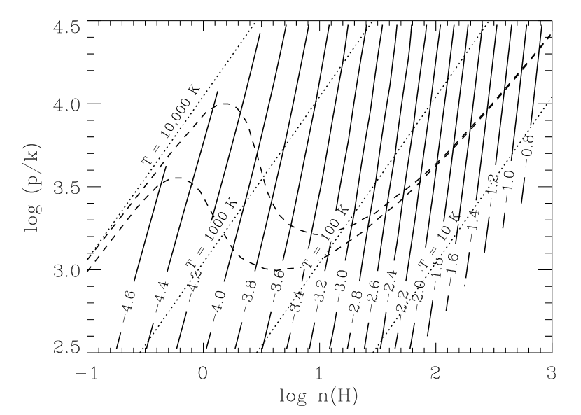
Figure 6: Expected values of $\log n({\rm C~{}I_{\rm total}})-\log n({\rm C~{}II})$ as a function of the parameters $\log(p/k)$ and $\log n({\rm H})$, found by solving Eq. 4. Other lines in the diagram are described in the caption for Fig. 4.

By comparing the contours in Figs. 4 and 6, it is clear that if $\alpha$ Del were to have $f1$ equal to the nominal value of 0.20 (for pure thermal broadening of the lines), the temperature must be equal to or less than 150 K to give an expected yield of ${\rm C~{}I_{\rm total}}$ that is at least as large as the observed value. If $f1$ is as high as the $+1\sigma$ limit, the temperature could be as high as 250 K. The upper limit for $T$ if $f1$ is at its $-1\sigma$ limit is 90 K. These temperature limits are substantially lower than those set by the width of the Na I absorption feature.

For $\lambda$ Lup, the strong, central peak of the S II absorption matches the velocity of the C I profile (see Fig. 5). The S II associated with this peak has a column density $N({\rm S~{}II})=1.2\times 10^{15}\,{\rm cm}^{-2}$. (It is reasonable to consider the gas giving absorptions at velocities on either side of this peak to arise from unrelated material.) Using reasoning identical to that applied to $\alpha$ Del, one finds for $\lambda$ Lup that $N({\rm H~{}I})=6.2\times 10^{19}\,{\rm cm}^{-2}$, $N({\rm C~{}II})=8.7\times 10^{15}\,{\rm cm}^{-2}$, and $\log N({\rm C~{}I}_{\rm total})-\log N({\rm C~{}II})=-3.81$. Clearly, the restriction on $T$ for $\lambda$ Lup is not as stringent as for $\alpha$ Del: a limit $T<2700\,$K arises from the interception of a line corresponding to $f1=0.19$ (nominal value) with the expectation $\log N({\rm C~{}I}_{\rm total})-\log N({\rm C~{}II})=-3.81$. This limit is only mildly more restrictive than the one that arises from the line width of Na I. For $f1=0.05$ (the $-1\sigma$ limit) the limiting temperature drops to 350 K.

6.2.2 Lower Limits

A task which now remains is to confine the allowable temperatures on the low side, since, as with high temperatures, arbitrarily high pressures could occur if $T$ were permitted to be arbitrarily low (again, see Fig. 4). In order to realize such a constraint, one may consider the sequence of temperatures at different densities predicted for thermal equilibrium in the interstellar medium. Wolfire et al. (1995) calculated equilibria for the diffuse phases of interstellar material for various assumptions. The two curved, dashed lines in Fig. 4 show the outcomes for their predictions based on heating rates for material shielded by absorbing columns $N({\rm H~{}I})=10^{18}$ (upper curve) and $10^{19}\,{\rm cm}^{-2}$ (lower curve), using cooling rates based on normal grain and heavy element abundances. According to Field’s (1965) thermal stability criterion, stable phases of the interstellar medium should be located only along portions of the equilibrium curves that have a positive slope in the $\log p$ vs. $\log n$ diagram (Field, Goldsmith, & Habing 1969; Shull 1987; Begelman 1990). In a simplistic application of this principle, one would predict that stable phases would exist only at slightly below 10,000 K (left-hand branch) or in the range $30<T<300\,$K (right-hand branch). In reality, this picture is only partly correct. On the one hand, observations of 21-cm emission and absorption in directions toward extragalactic sources indicate that about half of the H I in the diffuse medium violates this condition (Heiles 2001). The data show strong evidence that gas can often be found at temperatures that are intermediate between the two (positive-slope) equilibrium curves, an effect that is probably attributable to the effects of mixing of the two extremes in a regime strongly dominated by turbulence (Vázquez-Semadeni, Gazol, & Scalo 2000; Gazol et al. 2001). On the other hand, the observations generally show that the lowest H I temperatures coincide with the theoretical expectations. While broad surveys of emission with superposed absorption highlight a few, selected locations where spin temperatures are below 30 K (Gibson et al. 2000; Knee & Brunt 2001), the sight lines toward extragalactic sources offer a chance to sample random volumes: the survey of emission and absorption toward these sources reported by Heiles (2001) and Heiles & Troland (2002) reveals that only about 3.7% of the cold, neutral medium is at temperatures below $25\,$K. In short, the 21-cm data indicate that a good working assumption is that $T$ is usually above the right-hand branch of the thermal equilibrium curve, and violations of the lower limit defined by this curve are rare. For this reason, it is reasonable to regard the nearly coincident dashed lines on the right-hand side of Fig. 4 as a good representation for the lowest probable temperatures for different pressures.

7 Conclusions and Possible Interpretations

A synthesis of the conclusions presented earlier is shown in Figure 7, again in the representation of $\log(p/k)$ vs. $\log n({\rm H})$. To constrain the allowed physical conditions, the outcomes presented in Table 3 for the fine-structure population ratios of C I, represented by the parameter $f1$, must be supplemented by intersecting lines representing temperature limits derived in §6.2. Of these limits, the upper bounds derived from the measurements of the Na I line widths by other investigators are the most direct and reliable. However these measurements are valuable only for the cases of $\gamma$ Ori and $\delta$ Cyg. Alternative means for limiting $T$, such as using the thermal equilibrium curve to define a lower bound and the carbon ionization equilibrium for an upper bound, are indirect and subject to less certain theoretical assumptions.

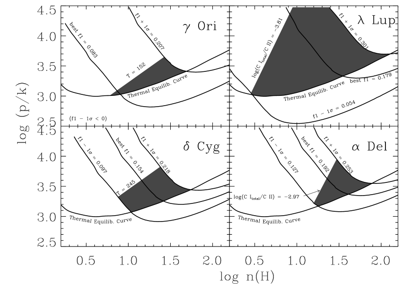
Figure 7: Allowed combinations of $\log(p/k)$ and $\log[n({\rm H})]$ permitted by the $\pm 1\sigma$ error limits for $f1$ for the C I-absorbing regions in front of the four targets. Intersecting constraints arise from the thermal equilibrium curve for an external absorbing column $N({\rm H~{}I})=10^{19}\,{\rm cm}^{-2}$ calculated by Wolfire, et al (1995), and temperature limits defined either from the Doppler width of Na I absorption lines or, alternatively, the requirement that the expected yield of ${\rm C~{}I_{total}}$ relative to C II from the condition of ionization equilibrium (Eq. 4) is as least as much as actually observed. General layouts of the expected C I fine-structure population ratios and ${\rm C~{}I_{\rm total}/C~{}II}$ ionization equilibria are shown in Figs. 4 and 6, respectively.

It should be noted that for each case the lines that border the allowed (shaded) regions do not enclose the worst possible deviations. For instance, the $f1$ limits represent only $\pm 1\sigma$ deviations. The temperature constraints from the width of the Na I absorption lines do not include possible errors in measurement, since they are difficult to assess. The theoretical limits based on thermal equilibria or the expected fractional abundances of carbon in neutral form are only as good as the assumptions that were incorporated into their respective developments. In spite of these shortcomings, when three of the stars (those other than $\lambda$ Lup) are examined collectively, they indicate that clouds within the Local Bubble have thermal pressures in the range $10^{3}<p/k<10^{4}\,{\rm cm}^{-3}\,$K.

From the introductory remarks presented in §1, it is clear that the most interesting limit on pressure is the upper one. Any single case is not compelling enough to support the proposal that $p/k<10^{4}\,{\rm cm}^{-3}\,$K, since deviations in excess of $1\sigma$ in a particular direction can be expected to occur 16% of the time. Nevertheless, if one supposes that all clouds within the Local Bubble have a single representative pressure, it is difficult to imagine that all of the random observational errors would conspire to mislead us to believe that $p/k<10^{4}\,{\rm cm}^{-3}\,$K when in reality the pressure is much higher than this value. The result for $\lambda$ Lup is not helpful in constraining $p$ on the high side, but at least it shows an outcome on the low side that is consistent with those of the other stars. As for systematic errors, the only easily identifiable ones are possible errors in the relative $f$-values of the C I and C I* transitions or errors in the parameters used to develop the predicted values of $f1$, such as the collisional rate constants or spontaneous radiative decay rates.

It is apparent from this study that a seemingly large disparity in pressure between neutral clouds embedded in the Local Bubble and the surrounding hot gas is a general phenomenon and not just confined to the LIC around the Sun. Possible solutions to the dilemma posed by the apparent pressure imbalance may arise from the following considerations:

1. Perhaps the clouds have not had enough time to respond fully to a sudden increase in external pressure that happened during the event(s) that created the LB, perhaps some $10^{5}-10^{7}$ yr ago (Cox & Reynolds 1987). If this is the case, each cloud is in an intermediate condition where a shock is still progressing from the periphery of the cloud, perhaps well outside the portion containing the C I, to its center. However, this explanation is not satisfactory for the LIC, since the distance from the Sun to the closest boundary divided by the sound speed is less than $10^{4}$ yr.

2. Perhaps magnetic fields within the clouds provide the support needed to counteract the high pressure from the outside. An upper limit $B<3\mu$G for the magnetic field just outside the heliosphere (Gloeckler, Fisk, & Geiss 1997) diminishes the attractiveness of this explanation in the case of the LIC.

3. Additional contributions to the clouds’ internal pressures might arise from turbulent motions. However, the narrowness of the Na I lines observed for $\gamma$ Ori and $\delta$ Cyg lowers the prospects for this proposal. For instance, if one uses the limit $n({\rm H})<10^{1.7}\,{\rm cm}^{-3}$ shown in Fig. 7 and assumes the Na I lines are broadened only by turbulence, one finds that $p_{\rm turb}/k=\rho b^{2}/2k<470$ and $800\,{\rm cm}^{-3}\,$K for $\gamma$ Ori and $\delta$ Cyg, respectively.

4. Perhaps the measurements of the thermal pressure for the hot gas in the Local Bubble were incorrect because they relied on either inaccurate models for the line emission or the assumption that the radiation from the hot plasma is emitted under equilibrium conditions. For a plasma that is cooling very rapidly, perhaps through adiabatic expansion, the x-rays may come principally from delayed recombinations in cooler gas, rather than collisional excitations at higher temperatures (Breitschwerdt & Schmutzler 1994). Apart from this theoretical proposal, there have also been persistent difficulties in reconciling measurements of x-ray and EUV line emission with models for a hot plasma in collisional equilibrium and with cosmic abundance ratios of the heavier elements (Jelinsky, Vallerga, & Edelstein 1995; McCammon et al. 2002). In trying to understand the soft x-ray spectrum measured by the Diffuse X-ray Spectrometer (DXS), Sanders et al. (2001) even explored models with depleted element abundances and nonequilibrium conditions arising from either rapid heating or cooling. From their inability to achieve reasonable fits of these more complex models with their data, they suggested that the discrepancies might arise from inaccurate atomic data which were used to predict the expected emission line strengths. If these models are in need of revision, then one might question the earlier estimates of hot gas emission measures from low resolution surveys of x-ray emission that led to the finding that $p/k>10^{4}\,{\rm cm}^{-3}$K within the LB.

Appendix A Fixed-Pattern Noise Analysis

A.1 Equations

The discussion here addresses the problem of disentangling the detector’s fixed pattern response function from the spectrum that moves, on the basis of information presented in the separate exposures. The analysis method solves for the two functions, but with the actual work being carried out in the Fourier Transform domain. This method has two important features. First, it offers a direct evaluation of the solutions, rather than relying on an initial guess for the two functions that is followed by iterations that gradually improve the representations until they converge toward consistent representations. Second, by exploring the properties of equations that operate in the Fourier domain, we gain insights on some near singular conditions that, in some practical circumstances, give poorly defined results when the shift dimensions have common factors in wavelength. This problem, discussed in §A.2, warns us of some potential dangers of programming shifts that are of uniform magnitude, as was intended for the FP-SPLIT routines on GHRS.

An individual spectrum $F(\lambda)$ recorded by a spectrograph consists of the actual spectrum $A(\lambda)$ multiplied by the pattern function $P(\lambda)$, plus a noise contribution arising from statistical fluctuations in the recorded photoevents. For the Digicon detector on GHRS, $P(\lambda)$ has the appearance of a function that, over large scales, is nearly constant, but with a high frequency granularity having an amplitude of a few percent. However, occasionally there are flaws in the photocathode that give much larger spikes (Ebbets 1992). In the reference frame of the detector’s photocathode, separate recordings of $F_{i}(\lambda)$ using the FP-SPLIT routine consist of the stationary pattern function $P(\lambda)$ with different superpositions of the actual spectrum $A(\lambda)$ having offsets with magnitudes $\delta_{i}$ in the wavelength direction, where the subscript $i$ differentiates the separate exposures. The magnitudes of $\delta_{i}$ may be determined by either cross correlating the exposures (for a spectrum with many narrow features) or comparing the offsets of positions of a strong line. The latter is recommended over the former if a single, narrow feature is present, with the rest of the spectrum being mostly random noise or much broader features.

As a first step in the analysis, we can reformulate the observed spectrum $F(\lambda)$ in terms of its logarithm, so that the mixing of two functions represented by $P(\lambda)$ and $A(\lambda)$ is a simple linear sum, $\log[P(\lambda)]+\log[A(\lambda-\delta_{i})]$. A restriction that should be imposed is that downward excursions of both $P(\lambda)$ and $A(\lambda)$ are not very large compared with the average signal levels. If this condition is violated, the negative dips can have a disproportionately large influence on the outcome, especially because the analysis works in the Fourier domain where large (negative) $\delta$-functions can have a global effect. For $P(\lambda)$ this restriction to small amplitudes is generally satisfied for GHRS, except at the locations of serious flaws in the photodiode array (which are normally corrected out beforehand). For the actual spectrum $A(\lambda)$, we require that there are no very deep absorption features. (Methods for overcoming problems with deep features in the spectrum will be discussed very briefly in §A.2.)

In the Fourier domain we define the real and imaginary parts of the pattern’s transform by the functions in inverse wavelength $\omega$,

$$p_{x}(\omega)=\Re\bigl{\{}{\cal F}[\log P(\lambda)]\bigr{\}}$$ (A1)

and

$$p_{y}(\omega)=\Im\bigl{\{}{\cal F}[\log P(\lambda)]\bigr{\}}\ ,$$ (A2)

where $\cal F$ is the Fourier transform operator. For $F(\lambda)$ and $A(\lambda)$ we designate the functions $f_{x}$, $f_{y}$, $a_{x}$ and $a_{y}$ in the same manner and allow for the fact that separate recordings will have different phase shifts for $a$ that are invoked by multiplying the zero-shift, complex function $a_{x}(\omega)+ia_{y}(\omega)$ by a factor $\exp(-2\pi i\omega\delta_{i})$.

The best solutions for $p_{x}(\omega)$, $p_{y}(\omega)$, $a_{x}(\omega)$, and $a_{y}(\omega)$ may be evaluated at each $\omega$ independently by solving for the smallest possible sum $Q^{2}$ of the squared real and imaginary residuals

$$Q^{2}_{x}=\sum_{i=1}^{n}(a_{x}\cos\Delta_{i}+a_{y}\sin\Delta_{i}+p_{x}-f_{x,i})^{2}$$ (A3)

and

$$Q^{2}_{y}=\sum_{i=1}^{n}(-a_{x}\sin\Delta_{i}+a_{y}\cos\Delta_{i}+p_{y}-f_{y,i})^{2}~{},$$ (A4)

where $\Delta_{i}$ is an abbreviation for $2\pi\omega\delta_{i}$. This minimum is achieved by setting the partial differentials of $Q^{2}$ with respect to the four unknowns $a_{x}$, $a_{y}$, $p_{x}$, and $p_{y}$ equal to zero. If ${\bf u}(\omega)$ represents a vector of these respective unknowns at each $\omega$, we must solve a system of 4 linear equations

$${\bf C}(\omega)\cdot{\bf u}(\omega)={\bf b}(\omega)$$ (A5)

where the coefficients of $C_{i,j}$ of the matrix C and $b_{i}$ of the vector b are listed in Table 4.

Table 4: Coefficients  for the Matrix and Vector in Equation A5

Term	$C_{i,j}$					$b_{i}$
	$i$	$j=1$	$j=2$	$j=3$	$j=4$
$\partial Q^{2}\over\partial a_{x}$	1	$n$	0	$\sum\cos\Delta_{i}$	$-\sum\sin\Delta_{i}$	$\sum f_{x,i}\cos\Delta_{i}-\sum f_{y,i}\sin\Delta_{i}$
$\partial Q^{2}\over\partial a_{y}$	2	0	$n$	$\sum\sin\Delta_{i}$	$\sum\cos\Delta_{i}$	$\sum f_{x,i}\sin\Delta_{i}+\sum f_{y,i}\cos\Delta_{i}$
$\partial Q^{2}\over\partial p_{x}$	3	$\sum\cos\Delta_{i}$	$\sum\sin\Delta_{i}$	$n$	0	$\sum f_{x,i}$
$\partial Q^{2}\over\partial p_{y}$	4	$-\sum\sin\Delta_{i}$	$\sum\cos\Delta_{i}$	0	$n$	$\sum f_{y,i}$

After solving for each vector ${\bf u}(\omega)$ over all $\omega$, one simply evaluates the inverse Fourier transforms of the two pairs of terms, $u_{1}(\omega)+iu_{2}(\omega)$ and $u_{3}(\omega)+iu_{4}(\omega)$ to recover the best representations of $A(\lambda)$ and $P(\lambda)$, respectively.

A.2 Limitations

Large increases in the magnitudes of terms in the error matrices $[{\bf C}(\omega)]^{-1}$ at certain frequencies indicate places where the solutions are ill-defined. As one would expect, the outcomes for frequencies whose inverses are much larger than the total span of the $\delta_{i}$ are not well determined. The solutions for $A(\lambda)$ and $P(\lambda)$ can exhibit very broad, spurious undulations (of opposite sign), as an outcome of the analysis program’s attempt to reconcile small differences in the low-frequency components in the observed spectra arising simply from noise and subtle systematic errors. As a practical matter, it is reasonable to assign artificially a condition that any low-frequency components of the observed spectra must arise from either the source spectrum $A(\lambda)$ or the detector response $P(\lambda)$. A similar quandary arises for certain frequencies where integral numbers of sinusoidal variations in the spectrum can exactly match the spacings between all of the $\delta_{i}$. One consequence of this phenomenon is that the programmed intent of having equal step sizes the FP-SPLIT routine for GHRS was a misguided one. Fortunately, in practice the step sizes usually turn out to be not quite equal, and this removes the degeneracies of the solutions.

The presence of deep absorption features in a spectrum poses special difficulties. At the locations of these features, the logarithms of $F(\lambda)$ surge to very large negative values, becoming even uncomputable in the bottoms of lines where the absorption is total. One must acknowledge that there is no way to determine $P(\lambda)$ at locations where less than two of the spectra have non-zero fluxes. Inelegant but nevertheless workable methods of avoiding irregularities in the computations include adding a small offset to the spectrum so that zero intensities are never encountered or, alternatively, eradicating the line and replacing it with a continuum intensity level.

References

- (1)
- (2) Begelman, M. C. 1990, in The Interstellar Medium in Galaxies, ed. H. Thronson & M. Shull (Dordrecht: Kluwer), p. 287
- (3)
- (4) Berghöfer, T. W., Bowyer, S., Lieu, R., & Knude, J. 1998, ApJ, 500, 838
- (5)
- (6) Blades, J. C., Wynne-Jones, I., & Wayte, R. C. 1980, MNRAS, 193, 849
- (7)
- (8) Breitschwerdt, D., & Schmutzler, T. 1994, Nat, 371, 774
- (9)
- (10) Burrows, D. N., & Guo, Z. 1998, in The Local Bubble and Beyond, ed. D. Breitschwerdt, M. J. Freyberg & J. Trümper (Berlin: Springer), p. 279
- (11)
- (12) Cardelli, J. A. 1995, in Calibrating Hubble Space Telescope: Post Servicing Mission, ed. A. Koratkar & C. Leitherer (Baltimore: Space Telescope Science Inst.), p. 173
- (13)
- (14) Cardelli, J. A., & Ebbets, D. 1994, in Calibrating Hubble Space Telescope, ed. J. C. Blades & S. J. Osmer (Baltimore: Space Telescope Science Inst.), p. 322
- (15)
- (16) Cardelli, J. A., Ebbets, D. C., & Savage, B. D. 1993, ApJ, 413, 401
- (17)
- (18) Cardelli, J. A., Savage, B. D., Bruhweiler, F. C., Smith, A. M., Ebbets, D. C., Sembach, K. R., & Sofia, U. J. 1991, ApJ, 377, L57
- (19)
- (20) Cardelli, J. A., Mathis, J. S., Ebbets, D. C., & Savage, B. D. 1993, ApJ, 402, L17
- (21)
- (22) Cardelli, J. A., Meyer, D. M., Jura, M., & Savage, B. D. 1996, ApJ, 467, 334
- (23)
- (24) Cox, D. P., & Reynolds, R. J. 1987, ARA&A, 25, 303
- (25)
- (26) Crawford, I. A. 1991, A&A, 247, 183
- (27)
- (28) Ebbets, D. 1992, Final Report of the Science Verification Program for the Goddard High Resolution Spectrograph for the Hubble Space Telescope, (Boulder: Ball Aerospace Systems Group), pp. 4-34 to 4-36
- (29)
- (30) Federman, S. R., Sheffer, Y., Lambert, D. L., & Gilliland, R. L. 1993, ApJ, 413, L51
- (31)
- (32) Ferlet, R. 1999, A&A Rev., 9, 153
- (33)
- (34) Field, G. B. 1965, ApJ, 142, 531
- (35)
- (36) Field, G. B., Goldsmith, D. W., & Habing, H. J. 1969, ApJ, 155, L149
- (37)
- (38) Fitzpatrick, E. L., & Spitzer, L. 1994, ApJ, 427, 232
- (39)
- (40) — 1997, ApJ, 475, 623
- (41)
- (42) Gaustad, J. E., & Van Buren, D. 1993, PASP, 105, 1127
- (43)
- (44) Gazol, A., Vázquez-Semadeni, E., Sánchez-Salcedo, F. J., & Scalo, J. 2001, ApJ, 557, L121
- (45)
- (46) Gibson, S. J., Taylor, A. R., Higgs, L. A., & Dewdney, P. E. 2000, ApJ, 540, 851
- (47)
- (48) Gloeckler, G., Fisk, L. A., & Geiss, J. 1997, Nat, 386, 374
- (49)
- (50) Gry, C., & Jenkins, E. B. 2001, A&A, 367, 617
- (51)
- (52) Heiles, C. 2001, ApJ, 551, L105
- (53)
- (54) Heiles, C., & Troland, T. H. 2002, preprint
- (55)
- (56) Hobbs, L. M., York, D. G., & Oegerle, W. 1982, ApJ, 252, L21
- (57)
- (58) Hoffleit, D., & Jaschek, C. 1982, The Bright Star Catalogue, 4th ed., (New Haven: Yale U. Obs.)
- (59)
- (60) Howk, J. C., Savage, B. D., & Fabian, D. 1999, ApJ, 525, 253
- (61)
- (62) Howk, J. C., & Sembach, K. R. 1999, ApJ, 523, L141
- (63)
- (64) Jelinsky, P., Vallerga, J. V., & Edelstein, J. 1995, ApJ, 442, 653
- (65)
- (66) Jenkins, E. B. 1996, ApJ, 471, 292
- (67)
- (68) Jenkins, E. B., Jura, M., & Loewenstein, M. 1983, ApJ, 270, 88
- (69)
- (70) Jenkins, E. B., & Shaya, E. J. 1979, ApJ, 231, 55
- (71)
- (72) Jenkins, E. B., & Tripp, T. M. 2001, ApJS, 137, 297
- (73)
- (74) Jenkins, E. B., & Wallerstein, G. 1995, ApJ, 440, 227
- (75)
- (76) Jenkins, E. B., Silk, J., Wallerstein, G., & Leep, E. M. 1981, ApJ, 248, 977
- (77)
- (78) Jenkins, E. B., Tripp, T. M., Fitzpatrick, E. L., Lindler, D., Danks, A. C., Beck, T. L., Bowers, C. W., Joseph, C. L., Kaiser, M. E., Kimble, R. A., Kraemer, S. B., Robinson, R. D., Timothy, J. G., Valenti, J. A., & Woodgate, B. E. 1998, ApJ, 492, L147
- (79)
- (80) Keenan, F. P. 1989, ApJ, 339, 591
- (81)
- (82) Kimble, R. A. et al. 1998, ApJ, 492, L83
- (83)
- (84) Knee, L. B. G., & Brunt, C. M. 2001, Nat, 412, 308
- (85)
- (86) Lallement, R. 1998, in Proc. IAU Colloq. 166: The Local Bubble and Beyond, ed. D. Breitschwerdt, M. J. Freyberg & J. Trümper (Berlin: Springer), p. 19
- (87)
- (88) Leitherer, C. 2001, Space Telescope Imaging Spectrograph Instrument Handbook for Cycle 10, 5.1 ed., (Baltimore: Space Telescope Science Institute)
- (89)
- (90) Lindler, D., & Bowers, C. 2000, BAAS, 32, 1418
- (91)
- (92) Maíz-Apellániz, J. 2001, ApJ, 560, L83
- (93)
- (94) McCammon, D. et al. 2002, astro-ph, 0205012,
- (95)
- (96) Morton, D. C. 1991, ApJS, 77, 119
- (97)
- (98) Ochsenbein, F., Bauer, P., & Marcout, J. 2000, A&AS, 143, 23
- (99)
- (100) Perryman, M. A. C., Lindegren, L., Kovalevsky, J., Hog, E., Bastian, U., Bernacca, P. L., Crèze, M., Donati, F., Grenon, M., Grewing, M., van Leeuwen, F., van der Marel, H., Mignard, F., Murray, C. A., Le Poole, R. S., Schrijver, H., Turon, C., Arenou, F., Froeschlé, M., & Petersen, C. S. 1997, A&A, 323, L49
- (101)
- (102) Puyoo, O., & Ben Jaffel, L. 1998, in The Local Bubble and Beyond, ed. D. Breitschwerdt & M. J. Freyberg (Berlin: Springer), p. 29
- (103)
- (104) Redfield, S., & Linsky, J. L. 2000, ApJ, 534, 825
- (105)
- (106) Sanders, W. T., Edgar, R. J., Kraushaar, W. L., McCammon, D., & Morgenthaler, J. P. 2001, ApJ, 554, 694
- (107)
- (108) Sembach, K. R., & Savage, B. D. 1992, ApJS, 83, 147
- (109)
- (110) Sfeir, D. M., Lallement, R., Crifo, F., & Welsh, B. Y. 1999, A&A, 346, 785
- (111)
- (112) Shull, J. M. 1987, in Interstellar Processes, ed. D. J. Hollenbach & H. A. Thronson (Dordrecht: Reidel), p. 225
- (113)
- (114) Shull, J. M., & Van Steenberg, M. 1982, ApJS, 48, 95
- (115)
- (116) Slettebak, A. 1982, ApJS, 50, 55
- (117)
- (118) Smith, A. M., Bruhweiler, F. C., Lambert, D. L., Savage, B. D., Cardelli, J. A., Ebbets, D. C., Lyu, C.-H., & Sheffer, Y. 1991, ApJ, 377, L61
- (119)
- (120) Smith, R. K., & Cox, D. P. 2001, ApJS, 134, 283
- (121)
- (122) Snowden, S. L., Cox, D. P., McCammon, D., & Sanders, W. T. 1990, ApJ, 354, 211
- (123)
- (124) Snowden, S. L., Egger, R., Finkbeiner, D. P., Freyberg, M. J., & Plucinsky, P. P. 1998, ApJ, 493, 715
- (125)
- (126) Sofia, U. J., Fitzpatrick, E. L., & Meyer, D. M. 1998, ApJ, 504, L47
- (127)
- (128) Sofia, U. J., & Jenkins, E. B. 1998, ApJ, 499, 951
- (129)
- (130) Sofia, U. J., Cardelli, J. A., Guerin, K. P., & Meyer, D. M. 1997, ApJ, 482, L105
- (131)
- (132) Spitzer, L., & Fitzpatrick, E. L. 1993, ApJ, 409, 299
- (133)
- (134) Thompson, G. I., Nandy, K., Jamar, C., Monfils, A., Houziaux, L., Carnochan, D. J., & Wilson, R. 1978, Catalogue of Stellar Ultraviolet Fluxes, (s.l.: Science Research Council)
- (135)
- (136) Uesugi, A., & Fukuda, I. 1981, in Data for Science and Technology, Proceedings of the Seventh International CODATA Conference Kyoto, Japan, 8-11 October 1980, ed. P. S. Glaeser (Oxford: Pergamon), p. 201
- (137)
- (138) Vallerga, J. V., Vedder, P. W., Craig, N., & Welsh, B. Y. 1993, ApJ, 411, 729
- (139)
- (140) Vázquez-Semadeni, E., Gazol, A., & Scalo, J. 2000, ApJ, 540, 271
- (141)
- (142) Vergely, J.-L., Ferrero, R. F., Siebert, A., & Valette, B. 2001, A&A, 366, 1016
- (143)
- (144) Weingartner, J. C., & Draine, B. T. 2001, ApJ, 563, 842
- (145)
- (146) Welsh, B. Y., Craig, N., Vedder, P. W., & Vallerga, J. V. 1994, ApJ, 437, 638
- (147)
- (148) Welty, D. E., Hobbs, L. M., & Kulkarni, V. P. 1994, ApJ, 436, 152
- (149)
- (150) Wiese, W. L., Fuhr, J. R., & Deters, T. M. 1996, Atomic Transition Probabilities of Carbon, Nitrogen, and Oxygen: A Critical Data Compilation, (Journal of Physical and Chemical Reference Data Monographs, 7), (Washington: American Chem. Soc. and American Phys. Soc. for NIST)
- (151)
- (152) Wolfire, M. G., Hollenbach, D., McKee, C. F., Tielens, A. G. G. M., & Bakes, E. L. O. 1995, ApJ, 443, 152