Boundary layer, accretion disk and X-ray variability in the luminous LMXBs.

Using Fourier frequency resolved X-ray spectroscopy we study short term spectral variability in luminous LMXBs. With RXTE/PCA observations of 4U1608–52 and GX340+0 on the horizontal/normal branch of the color-intensity diagram we show that aperiodic and quasiperiodic variability on $\sim$ sec – msec time scales is caused primarily by variations of the luminosity of the boundary layer. The emission of the accretion disk is less variable on these time scales and its power density spectrum follows $P_{\rm disk}(f)\propto f^{-1}$ law, contributing to observed flux variation at low frequencies and low energies only. The kHz QPOs have the same origin as variability at lower frequencies, i.e. independent of the nature of the ”clock”, the actual luminosity modulation takes place on the neutron star surface,

The boundary layer spectrum remains nearly constant in the course of the luminosity variations and is represented to certain accuracy by the Fourier frequency resolved spectrum. In the considered range $\dot{M}\sim(0.1-1)\dot{M}_{\rm Edd}$ it depends weakly on the global mass accretion rate and in the limit $\dot{M}\sim\dot{M}_{\rm Edd}$ is close to Wien spectrum with $kT\sim 2.4$ keV (in the distant observer’s frame). The spectrum of the accretion disk emission is significantly softer and in the 3–20 keV range is reasonably well described by a relativistic disk model with a mass accretion rate consistent with the value inferred from the observed X-ray flux.

1 Introduction

It is commonly accepted that in non-pulsating neutron star X-ray binaries the magnetic field of the neutron star is weak enough and the accretion disk can extend close to the surface of a neutron star. If the neutron star rotation frequency is smaller than the Keplerian frequency at the inner edge of the disk, a boundary layer will be formed near the surface of the neutron star in which the accreting matter decelerates and spreads over star’s surface (Sunyaev & Shakura, 1986; Kluzniak, 1988; Inogamov & Sunyaev, 1999; Popham & Sunyaev, 2001). For a non-rotating neutron star, in Newtonian approximation half of the energy release due to accretion would take place in the boundary/spread layer. The effects of the general relativity can increase this fraction, e.g. up to $\sim 2/3$ in the case of a neutron star with radius $R_{\rm NS}=3R_{\rm g}$ (Sunyaev & Shakura, 1986; Sibgatullin & Sunyaev, 2000). Rotation of the neutron star and deviations of the space-time geometry from Schwarzschild metric further modify the fraction of the energy released on the star’s surface. Consequently, a luminous spectral component, corresponding to the boundary layer emission is expected be present in the X-ray spectrum of a neutron star X-ray binary

X-ray observations of neutron star LMXBs in the high luminosity state reveal rather soft composite X-ray spectra. Based on theoretical expectations they are usually represented as a sum of two components attributed to the optically thick emission of the accretion disk (Shakura & Sunyaev, 1973) and of the boundary layer/neutron star surface (Mitsuda et al., 1984; White et al., 1988). The spectra of these two components are rather similar to each other and decomposition of the X-ray emission into the boundary layer and accretion disk components is often ambiguous, especially when based on the spectral information alone. Not surprisingly, the best fit parameters derived from the data of different instruments and, correspondingly, the inferred values of the physically meaningful quantities are often in contradiction to each other (e.g. Mitsuda et al., 1984; Di Salvo et al., 2001; Done et al., 2002). A robust and sufficiently model independent method of separating the boundary layer and disk emission is of interest.

Mitsuda et al. (1984) and Mitsuda & Tanaka (1986) studied pattern of spectral variability on the timescale of $\sim 10^{3}$ sec in luminous LMXBs and found that the observed spectra can be represented as a sum of two components, having drastically different variability properties: a strongly variable $\sim 2$ keV nearly blackbody component and a stable softer component. They interpreted the hard and soft components as emission from the neutron star surface and from the optically thick accretion disk respectively and concluded that the optically thick disk is stable on the timescales considered. The latter conclusion is in accord with the finding of Churazov et al. (2001), who showed that the same is true in the high luminosity state of the black hole binary Cyg X-1. On time scales $\la 10^{2}$ sec the fractional amplitude of variations of the disk emission is at least an order of magnitude lower than that of the hard Comptonized component. These results indicate that a low level of variability might be an intrinsic property of the optically thick accretion disk, independent of the nature of the compact object.

Figure 1: The color–intensity diagram of GX340+0. Dashed line polygons show the regions at the Horizontal and upper half of the Normal Branch used for the frequency resolved analysis.

Figure 2: Power spectrum of GX340+0 at the upper part of the Horizontal Branch of the color-intensity diagram.

As is well known (see van der Klis, 1986; van der Klis, 2000, for review), aperiodic variability of X-ray flux from LMXBs can be broadly divided into two main phenomena – continuum noise and quasi-periodical oscillations (QPO) with frequencies ranging from several mHz to more than a thousand Hz (e.g. Hasinger & van der Klis, 1989; van der Klis, 2000; Revnivtsev et al., 2001). Mitsuda et al. (1984) studied the difference between the spectra averaged at different intensity levels – that restricted the range of accessible time scales to $\ga 10^{3}$ sec. In this paper we will exploit the technique of Fourier frequency resolved spectroscopy (Revnivtsev et al., 1999) to study spectral variability of luminous LMXBs on a broad range of time scales, including kHz QPO.

As defined in Revnivtsev et al. (1999), the Fourier frequency resolved spectrum is the energy dependent rms amplitude in a selected frequency range, expressed in absolute (as opposite to fractional) units. A similar approach was used by Mendez et al. (1997) to study the energy spectrum of kHz oscillations in 4U0614+09. One of it’s advantages over simple fractional rms–vs.–energy dependence is the possibility to use conventional (i.e. response folded) spectral approximations in order to describe the energy dependence of aperiodic variability. One should keep in mind, however, that the interpretation of the frequency resolved spectra often is not straightforward and might strongly depend on a priori assumptions. Nevertheless, several applications of this technique to variability of black hole binaries gave meaningful results (e.g. Revnivtsev et al., 1999; Gilfanov et al., 2000).

Figure 3: The low (left) and high (right) frequency parts of the power spectrum of 4U1608 averaged over all data used for analysis. The power spectrum of the high frequency part, showing two kHz QPO peaks was obtained by “shift-and-add” method.

The simplest situation, when frequency resolved spectra can be easily interpreted is illustrated by the following example. Consider a two-component spectrum, in which one component is stable and the normalization of the other varies while it’s spectral shape is unchanged. In this case the shape of the frequency resolved spectrum would not depend on Fourier frequency and would be identical to the spectrum of the variable component. The spectrum of the non-variable component could, in principle, be determined by subtracting the frequency resolved spectrum from the average spectrum with appropriate renormalization. Importantly, in this example the X-ray flux in all energy channels will vary coherently and with zero time/phase lag between different energies. Presence of significant phase lag and/or Fourier frequency dependence of the frequency resolved spectra would indicate that a more complex pattern of spectral variability is taking place and interpretation is then less obvious. With few exceptions, phase lag between light curves in different energy bands in luminous LMXBs (e.g. Sco X-1, GX5-1, 4U1608–52, 4U0614+091 etc.) is usually small, $\Delta\phi\la{\rm few}\times 10^{-2}$, coherence is consistent with unity, (e.g. Vaughan et al., 1994, 1999; Dieters et al., 2000) and the fractional rms-vs-energy dependence similar at different Fourier frequencies (van der Klis, 1986). This suggests, that Fourier frequency resolved spectral analysis can be applied and its interpretation is sufficiently straightforward and model-independent.

The structure of the paper is as follows. We briefly describe the data in Sect. 2. In Sect. 3 we present the results of the observations, show that the frequency resolved spectra do not depend upon the Fourier frequency, and constrain the time lags between different energies. The initial observational results are summarized in Subsect. 3.3. In Sect. 4 we show that a particularly simple form of the spectral variability is required in order to satisfy the observational constraints – the flux variations in different energy channels must be related by a simple linear transformation. In Sect. 5 we compare the expected spectra of the disk and boundary layer emission with the frequency resolved spectra. We show that the observed aperiodic and quasiperiodic variability is primarily caused by variations of the luminosity of the boundary layer and its energy spectrum can be represented, to certain accuracy, by the frequency resolved spectra. In Sect. 6 we discuss the boundary layer emission spectrum, it’s dependence on the mass accretion rate and implications of these results for disk and boundary layer models. The results are summarized in Sect. 7.

2 The data

In order to investigate the spectral variability of neutron star LMXBs in the soft (high luminosity) state we have used the RXTE/PCA (Bradt et al., 1993) observations of one of the bright Z-sources (Hasinger & van der Klis 1989) GX340+0. Our choice was defined by the requirement that the PCA configuration combined sufficiently high energy resolution (large number of the energy channels) with good timing resolution and large total exposure time. We selected observations from proposal P20053 performed from Sep.21 to Nov.4, 1997 with total exposure time of $\approx$178 ksec. The PCA configuration provided 31 energy channels in the 3–20 keV energy band with 2 msec time resolution. The detailed timing analysis of these data was presented earlier by Jonker et al. (2000).

The intensity-color diagram of GX340+0 is presented in Fig. 1. The Fig. 2 shows an example of the power density spectrum, corresponding to the beginning of the horizontal branch on the intensity-color diagram. The prominent QPO peak at $\sim 25$ Hz corresponds to so called Horizontal Branch Oscillation (HBO).

The kHz QPOs are known to be rather weak in the case of GX340+0 (especially the upper kHz QPO), and the available data on the source did not have enough sensitivity to study them in detail. Therefore, to investigate the properties of two kHz QPOs and compare them with the lower frequency variability we chose another bright LMXB, 4U1608-52. The data of proposal P30062 provide energy and timing resolution adequate for this purpose. Detailed analysis of kHz QPOs in these observations was presented in Mendez et al. (1999, 2001). During these observations the source was in the high luminosity state and had two strong kHz QPO peaks at frequencies $\sim 600-800$ Hz and $\sim 900-1200$ and somewhat weaker QPO at $\sim$45 Hz (Fig. 3). Our aim is to compare the spectral variability corresponding to these three QPO components.

The reduction of the PCA data was performed with the help of standard tasks from FTOOLS/LHEASOFT, version 5.1. The spectral approximations were done using XSPEC. In all spectral fits the interstellar absorption was fixed at $NH=5\cdot 10^{22}$ cm^-2 and $NH=1\cdot 10^{22}$ cm^-2 for GX340+0 and 4U1608–52 respectively.

Figure 4: Average and frequency resolved spectra of GX340+0 in the Horizontal Branch (Z=0–1, see Fig. 1). The solid lines show the Comptonized emission spectrum rescaled to match the frequency resolved spectra and the high energy part of the average spectrum. The parameters of the Comptonized spectrum are best fit to the frequency resolved spectrum of the $\sim 25$ Hz QPO (Table 2).

Figure 5: GX340+0. Ratios of the frequency resolved spectra in various Fourier frequency bands to that of the 16–32 Hz band, corresponding to the Horizontal branch QPO. The data are from the Horizontal Branch of the color–intensity diagram (Z=0–1), i.e. the same as in Fig. 4. Note that the vertical scale is different in different panels.

3 Fourier frequency resolved spectra

3.1 Low frequency continuum and QPO

As is well known, the X-ray variability properties and parameters of Z-sources depend significantly on the spectral state of the source as given by its position on the Z-diagram, the highest level of variability being observed at the beginning of the Horizontal Branch (see e.g. Jonker et al. (2000)). Therefore throughout most of the paper we used the data averaged over Horizontal Branch of the color-intensity diagram (shown by a polygon in Fig. 1). The results for the normal branch are discussed in Sect. 6. The power spectrum of GX340+0 on the horizontal branch is shown in Fig. 2.

The Fourier frequency resolved spectra in several frequency bands corresponding to the band limited continuum noise component and the $\sim 25$ Hz QPO are shown in Fig. 4 along with the conventional spectrum of the source averaged over the same data. The ratios of the frequency resolved spectra to that of the QPO are presented in Fig. 5. The spectra and the ratios demonstrate that their shape depends on the Fourier frequency at low frequencies and becomes independent of the frequency at $f\ga 0.5$ Hz. Similar behaviour was found by van der Klis (1986) in the case of another bright LMXB – Z-source GX5–1. In particular, it was noted, that Horizontal Branch Oscillations and the low frequency noise have the same, hard, fractional rms spectrum and that at lower frequencies variabilty becomes softer.

The upper limits on the possible variations of the spectral shape with Fourier frequency depend on the photon energy and Fourier frequency and vary from $\sim 5\%$ to $\sim 25\%$ (Fig. 5). Note that in the $0.5\la f\la 30$ Hz frequency range these upper limits are determined by the statistical uncertainties only. At higher frequencies, $f\ga 30$ Hz, there might be an indication, although not statistically significant enough, of a frequency dependence of the spectral shape (lower panel in Fig. 5). Another conclusion from the data presented in Fig. 4, important for the following discussion, is that all frequency resolved spectra are significantly harder than the average source spectrum.

The phase lags as function of energy and Fourier frequency are shown in Fig. 6. No statistically significant phase lags were detected in the Horizontal Branch of GX340+0 with upper limit of $\Delta\phi\sim 10^{-2}$, where phase $\phi$ is normalized to the interval 0–1 (as opposed to $0-2\pi$).

Figure 6: Phase lags for GX340+0 in the Horizontal Branch of the color–intensity diagram (Z=0–1) as function of energy (upper panel) and Fourier frequency (lower panel). The energy dependent phase lags were computed in the 1–32 Hz frequency range, the frequency dependent lags are between 3–6.5 keV and 6.5–13 keV energy bands. The phase is normalized to 0–1 interval.

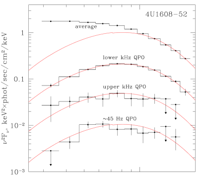
Figure 7: Upper panel: Average and frequency resolved spectra of 4U1608-52. The solid lines show Comptonized disk spectra rescaled to match the frequency resolved spectra and the high energy part of the average spectrum. The parameters of the Comptonization spectrum are the best fits to the frequency resolved spectrum of the lower kHz QPO (Table 2). Lower panel: Ratios of the spectra shown in the upper panel to the spectrum of lower kHz QPO.

3.2 kHz QPOs

As was mentioned above, the strength of the kHz QPOs in the power spectrum of GX340+0 is insufficient to study their frequency resolved spectra in detail. We therefore had to use for this purpose a different source – 4U1608-52 (Fig. 3). As the frequency of the kHz QPO varied during the RXTE observations we used “shift-and-add” technique (Mendez et al., 2001) in order to improve statistics. During the same observations the source showed a lower frequency QPO at $\sim$45 Hz as well.

The Fourier frequency resolved spectra of the two kHz QPOs and the HBO along with their ratios are shown in Fig. 7. As in the case of GX340+0, all three spectra are consistent with each other within the statistical uncertainties. The upper limits on possible variations of the spectral shape, however, are significantly less constraining, $\sim 30-50\%$ at best.

3.3 Summary of the observational results

The results of the above analysis can be summarized as follows:

1. The shape of the frequency resolved spectra does not depend or depends very weakly on the Fourier frequency. This includes the continuum band limited noise component, the Horizontal Branch QPO and the kHz QPOs. The constraints on possible Fourier frequency dependent variations of the spectral shape are rather stringent for the band limited noise and Horizontal Branch oscillations (GX340+0) – $\la 5-25\%$ in the $0.5\ga f\la 30$ Hz frequency range and significantly less restrictive for kHz QPO – $\la 30-50\%$.

2. The Fourier frequency resolved spectra at all frequencies are significantly harder than the average spectrum.

3. No statistically significant phase lags were detected in the case of GX340+0 with upper limits of $\Delta\phi\la 10^{-2}$ in the $0.1-30$ Hz frequency range and $3-17$ keV energy range.

4. At low Fourier frequencies, $f\la 0.5$ Hz, frequency dependent variations of the spectral shape become important – the frequency resolved spectra tend to become softer (GX340+0).

4 Interpretation of the Fourier frequency resolved spectra

We show here that independence of the frequency resolved spectra on the Fourier frequency and the smallness of the phase lags observed in majority of bright LMXBs (but see footnote 1) require a particularly simple form of the spectral variability.

The constancy of the spectral shape with Fourier frequency implies that the power spectrum $P(E,\omega)$ can be represented as a product of two functions, one of which depends on the energy and the other on the frequency only. For convenience we write $P(E,\omega)$ in the form:

$$P(E,\omega)=S^{2}(E)\times f^{2}(\omega)$$ (1)

where non-negative functions $S(E)$ and $f(\omega)$ can be directly determined from the frequency resolved spectra. The Fourier image of the light curve $F(E,t)$ is:

$$\hat{F}(E,\omega)=S(E)\times f(\omega)\times e^{i\phi(E,\omega)}$$ (2)

In the general case the complex argument $\phi(E,\omega)$ can depend both on Fourier frequency $\omega$ and energy $E$. If the phase lags between different energies are negligibly small, $\phi$ depends on the Fourier frequency only and the Fourier image of $F(E,t)$ is:

$$\hat{F}(E,\omega)=S(E)\times f(\omega)\times e^{i\phi(\omega)}$$ (3)

The light curve $F(E,t)$ can be computed via inverse Fourier transform of $\hat{F}(E,\omega)$:

$$F(E,t)=\int d\omega\hat{F}(E,\omega)e^{i\omega t}=$$

$$=S(E)\times\int d\omega f(\omega)e^{i\phi(\omega)}e^{i\omega t}=$$ (4)

$$=S(E)\times f(t)$$

An arbitrary function of energy can obviously be added to the above expression. Thus, the light curve at energy $E$ should satisfy the equation:

$$F(E,t)=S_{0}(E)+S(E)\times f(t)$$ (5)

i.e. the light curves at different energies are related by a linear transformation.

Eq. (5) significantly restricts the pattern of the spectral variability. Suppose that the spectrum of the source at any given moment of time can be represented as:

$$F(E,t)=S_{0}(E)+A(t)\times S(E,p(t))$$ (6)

where $A(t)$ is varying normalization, and $p(t)$ represents variations of the spectral parameter, on which the spectral flux at a given energy depends non-linearly (e.g. temperature, Thompson optical depth etc.). Using Taylor expansion:

$$F(E,t)=S_{0}(E)+A(t)\times S(E,p(t))=\hfill$$

$$=S_{0}(E)+A(t)\times S(E,p_{0})+$$

$$+A(t)\times\frac{\partial S(E,p_{0})}{\partial p}\times(p(t)-p_{0})+$$ (7)

$$+A(t)\times\frac{1}{2}\frac{\partial^{2}S(E,p_{0})}{\partial p^{2}}\times(p(t)-p_{0})^{2}+...$$

In order to satisfy Eq. (5), one of the following two conditions should be fulfilled: (i) $p(t)=p_{0}={\rm const}$, i.e. only the normalization varies with time, or (ii) the normalization is constant and variations of the spectral parameter are sufficiently small, so that the terms higher than linear in the Taylor expansion can be neglected. Simultaneous variations of comparable amplitude of the normalization and the spectral parameter (or of any two spectral parameters) would be consistent with observations only in the case of $A(t)\times(p(t)-p_{0})={\rm const}$ or in the case of specific shape of the power density spectrum of $A(t)$ (e.g. flat).

Figure 8: GX340+0: Coherence between the light curves in the 3–6.5 and 6.5–13 keV energy bands as function of frequency. No correction for the dead time effects has been made.

From Eq. (5) it follows that the coherence of the signals in any two energy bands is exactly unity, as they are related by a linear transformation. This is in agreement with the observed behaviour – as illustrated by an example of GX340+0, shown in Fig. 8, the coherence between the light curves in 3–6.5 and 6.5–13 keV energy bands is close to unity (see also Vaughan et al. 1994, 1999; Dieters et al. 2000 for results for other luminous LMXBs).

4.1 Case of black hole binaries

The spectral variability in the black hole binaries is more complicated than described by Eq. (5) because of the strong dependence of the shape of their frequency resolved spectra upon the Fourier frequency (Revnivtsev et al., 1999), rather than non-zero time/phase lags observed. Indeed, typical values of the phase lags measured for Cyg X-1 are negligible in this context, $\Delta\phi\la{\rm few}\times 10^{-2}$ (e.g Kotov, Churazov & Gilfanov, 2001). Therefore

$$\phi(E,\omega)=\phi_{0}(\omega)+\phi_{1}(E,\omega)$$

where

$$\phi_{1}(E,\omega)<<\phi_{0}(\omega)$$

and Eq. (3) and therefore Eq. (5) will hold with sufficient accuracy if condition of Eq. (1) is fulfilled.

5 Application to bright LMXBs

5.1 Frequency resolved spectra and nature of the variable component

Thus, observed properties of the luminous LMXBs (Sect. 3.3) require a particularly simple form of the spectral variability on time scales from $\sim$ sec to $\sim$ msec, described by Eq. (5). The term $S_{0}(E)$ in Eq. (5) represents constant (non-variable) part of the source spectrum and $f(t)$ represents either (i) variations of the normalization of the variable spectral component (e.g. Churazov et al., 2001) or (ii) small variations of the spectral parameter (e.g. Mendez et al., 1997).

If variability of the X-ray flux is caused mainly by variations of the normalization, it follows from Eq. (1), that the spectrum of the variable component $S(E)$ is identical in shape to the frequency resolved spectrum, i.e. can be directly determined from observations. The spectrum of the non-variable component can, in principle, be obtained subtracting $S(E)$ from the averaged spectrum with appropriate renormalization.

In the second case (small variations of the spectral parameter), the energy dependence of the frequency resolved spectrum $S(E)$ corresponds to the first derivative of the spectrum with respect to the parameter $p$, $\frac{\partial S(E,p)}{\partial p}$, which might differ significantly from the spectrum itself. Indeed, considering a Wien spectrum, $S(E,T)=E^{2}e^{-E/T}$, as an example (cf. Mendez et al. (1997)), the intensity variations are:

$$F(E,t)=S(E,T_{0})+\frac{\partial S(E,T_{0}))}{\partial T}\times\delta T(t)+...=$$ (8)

$$=S_{0}(E)+S_{0}(E)\times\frac{E}{T_{0}}\times\frac{\delta T(t)}{T_{0}}+...$$

Therefore in Eq. (5) $S(E)=S_{0}(E)\times E/T_{0}$, i.e. is harder than the average spectrum. It is intuitively obvious, however, that in order the linear expansion to be valid, the variations amplitude at any energy should be smaller than the average flux. Indeed, for the quadratic term in Eq. (7) to be neglectable, the following condition should be satisfied:

$$\frac{E}{T_{0}}\times\frac{\delta T(t)}{T_{0}}\ll 1$$ (9)

i.e. (cf. Eq. (8)) the frequency resolved spectrum in any frequency range and at any energy should be small in comparison with the average spectrum of the variable component. Equivalently, fractional rms of flux variations computed with respect to the average flux of the variable component (as opposite to the total average flux) should be less than 1.

In the first case identification of the variable component would be easy and unambiguous. However, no distinction between the two possibilities outlined above can be made based solely on the results of the frequency resolved analysis, and additional considerations should be taken into account.

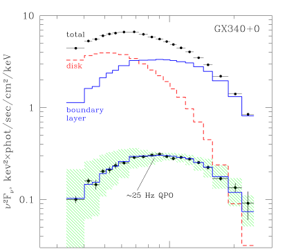
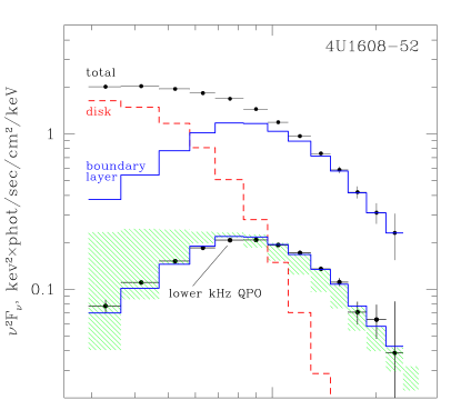
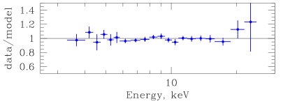
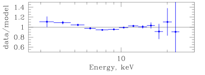
Figure 9: The average and frequency resolved spectra of GX340+0 (left) and 4U1608–52 (right). The GX340+0 data are from horizontal branch of the color–intensity diagram, i.e. the same as used before. The shaded area shows a plausible range of the boundary layer spectral shape calculated subtracting the predicted disk spectrum from the total spectrum and renormalizing the residual to the total energy flux of the frequency resolved spectrum (see Sect. 5.2 and Table 1 for details). The dashed histogram shows the accretion disk spectrum with parameters from Table 2 (Sect. 5.3), the upper solid histogram shows the difference between the total and accretion disk spectrum ($\approx$ boundary layer spectrum). The lower solid histogram is the same but scaled to the total energy flux of the frequency resolved spectrum. The lower panels show ratio of the frequency resolved spectrum to the lower histogram.

5.2 Emission from the boundary layer and accretion disk

Based on theoretical grounds (Sunyaev & Shakura, 1986; Kluzniak, 1988; Inogamov & Sunyaev, 1999; Popham & Sunyaev, 2001) and observational results (e.g. Mitsuda et al., 1984; Mitsuda & Tanaka, 1986; Gierlinski & Done, 2002) it is expected that in the case of accretion onto a slowly rotating weakly magnetized neutron star at sufficiently high mass accretion rates there are two major components of the accretion flow:

1. the optically thick accretion disk extending close to the surface of the neutron star or last marginally stable orbit

2. the boundary layer (e.g. Popham & Sunyaev, 2001) or spreading layer (Inogamov & Sunyaev, 1999) near the surface of the neutron star. In this layer the accreting matter decelerates to the spin frequency of the star and spreads over its surface.

Simple theoretical arguments, taking into account energy released in the accretion disk and in the boundary layer, and difference in their emitting areas suggest that the spectrum of the boundary layer emission should be noticeably harder than that of the optically thick accretion disk (e.g. Mitsuda et al., 1984; Grebenev & Sunyaev, 2002). Considering the restrictions on the character of spectral variability imposed by Eq. (5), it is natural to assume, that the observed variations of the X-ray flux should originate in one of these components. Furthermore, X-ray variability should be mainly caused by either variations of the total luminosity with nearly constant spectral shape or by small variations of the spectral shape. In order to distinguish between these possibilities and to identify the nature of the varying component we consider below theoretical expectations for the disk and boundary layer spectra and compare them with the observed frequency resolved spectra.

Due to complexity of the boundary/spreading layer problem, no models capable to directly predict its emission spectrum exist yet. An attempt of solve the radiation transfer problem using density and temperature profiles obtained in the hydrodynamical simulations (e.g. Popham & Sunyaev, 2001) failed to reproduce, even qualitatively, the observed X-ray spectra and demonstrated importance of the self-consistent treatment (Grebenev & Sunyaev, 2002).

Significantly better progress has been achieved with the spectra of accretion disks (Shakura & Sunyaev, 1973; Shimura & Takahara, 1995; Ross & Fabian, 1996). It has been shown that at sufficiently high mass accretion rates the effects of Compton scattering can be approximately accounted for by introducing a dilution factor to describe deviation of the spectra emitted at each radius of the disk from blackbody (Shimura & Takahara, 1995; Ross & Fabian, 1996). Additional modifications of the disk spectrum arise due to gravitational redshift and Doppler effects (Ebisawa et al., 1991; Ross & Fabian, 1996; Bhattacharyya et al., 2001). Relatively simple models of multicolor disk type which account for the effects of Compton scattering with a simple color-to-effective temperature ratio turned out to be successful in describing the accretion disk spectra observed in the high state of black hole systems (e.g. Ebisawa et al., 1991; Gierlinski et al., 1997).

Table 1: Range of parameters used to estimate plausible range of the accretion disk and boundary layer spectra (Fig. 9)

Parameter	GX340+0	4U1608-52
D, kpc	8.5–10.5	3.5–4.5
$F_{\rm 0.1-30\leavevmode\nobreak\ keV}$ 1	$2.7\cdot 10^{-8}$	$8.8\cdot 10^{-9}$
$\cos(i)$	0.3–0.7
$T_{\rm col}/T_{\rm eff}$	1.6–2.0
$\nu_{\rm NS},Hz$	0–700
$\eta_{\rm tot}$ 2	0.213–0.116
$f_{\rm disk}$ 2	0.26–0.57
$f_{\rm BL}$ 2	0.74–0.43

1 – absorption corrected, erg/s/cm²
2 – derived values of the total accretion efficiency and fraction of the energy released in the disk and boundary layer respectively, corresponding to the considered range of the neutron star spin frequency, for a $1.4M_{\sun}$ neutron star, EOS FPS (Sibgatullin & Sunyaev, 2000).

Therefore we use the predicted disk spectrum as a starting point and subtract it from the total spectrum in order to calculate expected spectrum of the boundary layer. To estimate the plausible range of the boundary layer spectra we investigate the parameter space of the accretion disk model. This approach enables one to predict the disk and the boundary layer spectra based on the observed X-ray flux and spectrum and very generic system parameters, such as neutron star spin frequency or the source distance. For this analysis we adopt the general relativistic accretion disk model by Ebisawa et al. (1991) (the “grad model” in XSPEC). The parameters of the model are: the source distance $D$, mass of the central object $M_{\rm NS}$, disk inclination angle $i$, the mass accretion rate $\dot{M}$ and the color-to-effective temperature ratio $f=T_{\rm col}/T_{\rm eff}$. The source distance was varied in the range 8.5–10.5 kpc (GX340+0) and 3.5-4.5 kpc (4U1608–52), the disk inclination – in the range of $\cos i=0.3-0.7$, color-to-effective temperature ratio – in the range 1.6-2.0 (Shimura & Takahara, 1995).

In order to estimate the plausible range of mass accretion rates we used the total accretion efficiency $\eta_{\rm tot}$ and relative energy release fractions of the disk, $f_{\rm disk}$, and the neutron star surface, $f_{\rm BL}$, calculated by Sibgatullin & Sunyaev (2000). These account exactly for the space-time metric around a neutron star with a given spin frequency and equation of state. In particular we used their results for a neutron star with gravitational mass of 1.4 $M_{\sun}$ described by FPS equation of state (their eqs. (1) and (2)). In computing the relation between the observed luminosity and the mass accretion rate we ignored the light bending and abberation effects, the real geometry of the spreading layer and shadow cast by the neutron star on the disk and boundary layer:

$$L_{\rm obs}=\left(d(i)f_{\rm disk}+d(\frac{\pi}{2}-i)f_{\rm BL}\right)\times\eta_{\rm tot}\dot{M}c^{2}$$ (10)

where emission diagram is described by Chandrasekhar–Sobolev law $d(i)\approx 3/7(1+2.06\cos i)\cos i$. The luminosity $L_{\rm obs}$ was computed from the absorption corrected fluxes extrapolated to 0.1–30 keV energy range. The total correction factor from observed 3–20 keV flux was $\sim 2$ in both cases. Therefore, unless a new spectral component appears outside the 3–20 keV PCA energy range, the uncertainty of the flux correction should not exceed few tens of per cent. The accretion efficiency $\eta_{\rm tot}$ and the disk and boundary layer fractions $f_{\rm disk}$ and $f_{\rm BL}$ depend, obviously, on the neutron star spin, which was varied in the range 0–700 Hz assuming that the neutron star and disk co-rotate.

The investigated range of the disk parameters is summarized in Table 1. Each predicted disk spectrum was subtracted from the total spectrum and the residual ($\approx$boundary layer spectrum) was normalized to the observed 3–20 keV energy flux of the frequency resolved spectrum. The resulting range of the boundary layer spectra for two sources is shown in Fig. 9 as the shaded area along with the average and frequency resolved spectra of the 25 Hz and kHz QPO and the best fit model described in Subsect. 5.3. The lower panels in Fig. 9 show ratio of the frequency resolved spectrum to predicted boundary layer spectrum. Different models of the disk emission, e.g. ignoring the relativistic effects (the “diskpn” model in XSPEC, Gierlinski et al. 1997) or model of Ross & Fabian (1996) which more accurately accounts for the Compton scattering effects, but assuming Newtonian dynamics, change the details but do not alter the general conclusion. The close similarity of the expected boundary layer and the observed frequency resolved spectra strongly suggests that X-ray variability is caused by variations of the luminosity of the boundary layer component. It also implies that the spectrum of the boundary layer emission does not change significantly in the course of these variations (cf. example given by Eq. (8)).

Figure 10: The energy dependence of the fractional rms of the kHz QPO in 4U1608–52. Flattening above $\sim 10$ keV indicates, that the energy spectrum of the oscillations at these energies has the same shape as the total spectrum.

On the other hand it is obvious from Fig. 9 that the disk spectrum is significantly softer and can not reproduce the observed frequency resolved spectrum. Qualitatively, this fact does not rule out the possibility that X-ray variability is due to variations of the disk emission spectrum. Indeed, variations of e.g. disk temperature can result in the frequency resolved spectra significantly different (in particular, harder, cf. Eq. (8)) than the average spectrum. However, as discussed in Sect. 5.1, in order to maintain constancy of the shape of the frequency resolved spectra and zero time lags between different energy channels it is required, that frequency resolved spectra in any frequency range are $\ll$ than the average spectrum of the variable component. This condition is obviously violated at $E\ga 10-15$ keV (Fig. 9 – cf. the disk and the frequency resolved spectra).

Considering the quick decline of the disk emission above $\sim 10$ keV, another test of the suggested interpretation might be the behavior of the frequency resolved spectrum (or fractional rms) at high energy, $\ga 10-15$ keV. Indeed, as at $E\ga 10-15$ keV the total spectrum is dominated by the boundary layer emission, the fractional rms in the above scenario is expected to become independent of the photon energy. Due to insufficient energy coverage this can not be checked in the case of GX340+0 where the disk temperature is rather high. Flattening of the fractional rms is clearly seen in 4U1608–52 (lower-most panel in Fig. 7 and Fig. 10), having $\sim 10$ times lower mass accretion rate and correspondingly lower disk temperature and softer disk spectrum. Similar behavior was observed by Mitsuda et al. (1984) for Sco X-1 using TENMA data.

Thus, we conclude that the bulk of the X-ray variability observed in GX340+0 and 4U1608–52 and, presumably, in other luminous LMXBs, on $\sim$ second – millisecond time scales is due to variations of the boundary layer luminosity. The shape of the boundary layer emission spectrum remains nearly constant in the course of these variations. Therefore the energy spectrum of the variable component – the frequency resolved spectrum should be representative, to some accuracy, of the spectrum of the boundary layer emission. This can be used to separate the boundary layer and the accretion disk contribution to the total spectrum and permits to check quantitatively the predictions the accretion disk and boundary layer models. It also opens the possibility to measure relative contributions of these two components of the accretion flow to the total observed X-ray emission.

Table 2: Parameters of the spectral modeling

Parameter	GX340+0	4U1608-52
D, kpc	8.5	4.0
NH, cm-2	$5\cdot 10^{22}$	$1\cdot 10^{22}$
$F_{\rm 3-20\leavevmode\nobreak\ keV}$ 1 erg/s/cm2	$1.4\cdot 10^{-8}$	$4.2\cdot 10^{-9}$
$F_{\rm 0.1-30\leavevmode\nobreak\ keV}$ 2 erg/s/cm2	$2.7\cdot 10^{-8}$	$8.8\cdot 10^{-9}$
$L_{\rm 0.1-30keV}$ 2 erg/s	$2.3\cdot 10^{38}$	$1.7\cdot 10^{37}$
$\dot{M}$ 3, g/s	$3.1\cdot 10^{18}$	$2.0\cdot 10^{17}$
QPO frequency resolved spectra ($\approx$boundary layer)4
power law with exponential cutoff (phabs$\times$cutoffpl)
$\alpha$	$-0.55\pm 0.16$	$-1.28\pm 0.13$
$E_{\rm f}$, keV	$3.3\pm 0.2$	$2.4\pm 0.1$
$\chi^{2}$/dof	13.9/16	4.8/9
Comptonization model (phabs$\times$comptt)
$kT_{\rm bb}$, keV	$1.3\pm 0.2$	$1.4\pm 0.4$
$kT_{\rm e}$, keV	$3.1_{-0.3}^{+0.9}$	$2.6_{-0.3}^{+\infty}$
$\tau$	$6.0_{-2.1}^{+1.8}$	$6.7_{-5.3}^{+5.7}$
$\chi^{2}$/dof	11.3/15	4.0/8
average spectra4
phabs$\times$(grad+pexrav+gaussian)
inclination5	$60\degr$	$70\degr$
$T_{\rm col}/T_{\rm eff}$ 5	1.7	1.8
$\dot{M}$, $10^{18}$ g/s	$3.0\pm 0.04$	$0.34\pm 0.01$
$\dot{M}/\dot{M}_{\rm Edd}$ 6	$\approx 0.9$	$\approx 0.1$
$\Omega/2\pi$	$0.27\pm 0.07$	$\la 0.1$
$EW$ 7, eV	$48\pm 10$	$147\pm 17$
$L_{\rm BL}/L_{tot}$, 3–20 keV	47%	57%

1 – observed; 2 – absorption corrected; 3 – calculated from the total unabsorbed luminosity using the accretion efficiency for the neutron star spin frequency of $\nu_{\rm NS}=500$ Hz (Sibgatullin & Sunyaev, 2000, see Sect. 5.2, Eq. (10)); 4 – the details of spectral modeling are given in Sect. 5.3; 5 – fixed at fudicial value; 6 – assuming $\dot{M}_{\rm Edd}=2\cdot 10^{38}/c^{2}\eta_{\rm disk}\approx 3.5\cdot 10^{18}$ g/s, where $\eta_{\rm disk}=0.066$ – accretion disk efficiency for $\nu_{NS}=500$ Hz and $M_{NS}=1.4M_{\sun}$; 7 – line energy and width were fixed at $E_{\rm line}=6.7$ keV and $\sigma_{\rm line}=0.5$ keV

5.3 Spectral modeling

As small variations of the spectral shape of the boundary layer emission in the course of flux variations can not be excluded and are likely to take place, the frequency resolved spectra represent the boundary layer emission with a certain accuracy only. This should be kept in mind while interpreting the spectral fitting results described in this subsection. However, the reasonable quality of the spectral fits and values of the spectral parameters for two sources with significantly different mass accretion rate provide additional indirect support to the main conclusion of this section.

Below we approximate the frequency resolved spectrum ($\approx$ spectrum of the boundary layer emission) with a plausible model and then fit the total spectrum adding the accretion disk component. This procedure is equivalent to subtracting the renormalized frequency resolved spectrum from the total spectrum, with the renormalization coefficient determined by requirement to minimize $\chi^{2}$.

The simplest models of the blackbody or Wien spectrum with $kT\sim 2-2.2$ keV, although they reproduce approximately the shape of the frequency resolved spectra, show statistically significant deviations from the data (Fig. 11) and give unacceptable value of $\chi^{2}$. Significantly better the spectra can be described by the Comptonized emission models (Sunyaev & Titarchuk, 1980; Poutanen & Svensson, 1996). Although simple Comptonization models are not expected to be directly applicable to the emission spectra emerging from the boundary layer, we give in Table 2 the best fit parameters for comptt model in XSPEC (Titarchuk, 1994) for easy comparison with other results. A convenient parameterization of the frequency resolved spectra is provided by a power law spectrum with exponential cut-off, which we will use for the following analysis of the average spectra.

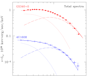
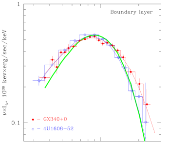
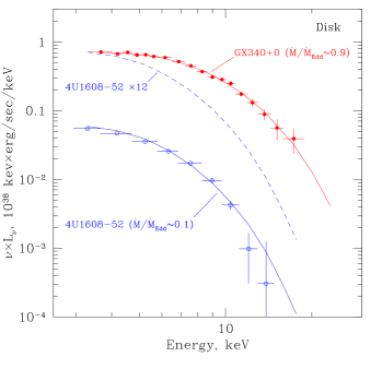
Figure 11: The absorption corrected average (upper panel), frequency resolved ($\approx$ boundary layer, middle) and accretion disk (lower) spectra of GX340+0 and 4U1608–52. The solid, dashed and dotted lines in the upper panel show the best fit total, boundary layer and accretion disk spectra. The thin solid lines in the middle panel are best fit Comptonized spectra, the thick grey line is Wien spectrum with $kt=2.1$ keV. The frequency resolved spectra are normalized to the same energy flux. The solid lines in the lower panel show best fit spectra of the accretion disk, the dashed line is 4U1608–52 spectrum multiplied by a factor of 12. See Table 2 for values of the spectral parameters.

As the second step, we approximate the average spectra by a two component model including the disk, boundary layer emission and the reflected component appearing due to reflection of the latter from the accretion disk: phabs$\times$(grad+pexrav+gaussian). The shape (but not the normalization) of the boundary layer emission was fixed at the values determined from approximation of the frequency resolved spectrum. The reflection was modeled using pexrav model (Magdziarz & Zdziarski, 1995) and a broad gaussian line at 6.4–6.7 keV. All parameters of the grad model were fixed except the mass accretion rate. The mass of the neutron star was fixed at 1.4$M_{\sun}$. The disk inclination angle and the color-to-effective temperature ratio were fixed at somewhat arbitrary, although reasonable, values, which were chosen to approximately minimize the residuals. Note, that presence of the line at $E\sim 6-7$ keV in the average spectrum is statistically significatly required by the data, especially in the case of 4U1608–52. The parameters of the spectral fits are summarized in the Table 2. The best fit models and different components are depicted Fig. 9 and 11. Although the $\chi^{2}$ values of the fits to the average spectra are in the range 3.0–4.5 per d.o.f. and are formally unacceptable, the models describe the observed total spectra (having very statistical significance, signal/noise$\sim 10^{2}-10^{3}$ per energy channel) reasonably well, with relative accuracy of $\la 1-2\%$ in the 3–20 keV band.

6 Discussion

The best fit values of the mass accretion rates obtained from the spectral fits agree, within a factor of $\la 1.7$ with the values predicted from the observed energy flux and the accretion efficiency expected for a neutron star with spin frequency of $\sim 500$ Hz (Eq. (10)). This fact is especially encouraging, as the two sources have accretion rates different by a factor of $\sim 10$ (Table 2). For such difference in the accretion rate the expected disk temperatures should differ by a factor for $\sim 1.7-1.8$, resulting in the different shape and total flux of the disk spectra (Fig. 11, lower panel). However, after the contribution of the boundary layer is accounted for, the relativistic disk emission model is capable of reproducing both spectral shape and normalization.

Despite large difference in the mass accretion rate in the two sources, the energy spectra of the boundary layer emission are very similar to each other. This is in line with the finding that variations of the boundary layer luminosity in the broad range of time scales from $\sim$sec to $\sim$msec are not accompanied by significant variations of the spectral shape. Similar behavior was found by Mitsuda et al. (1984) and Mitsuda & Tanaka (1986) on longer time scales of $\sim 10^{3}$ sec.

Due to short light travel time of the accretion disk in the vicinity of the neutron star, $\sim$msec, the reflected component, if originating in the inner disk, could contribute to the variable emission and cause deviation of the frequency resolved spectra from the true boundary layer spectrum. This can not be directly verified with the present data – upper limit on the equivalent width of the 6.4-6.7 keV line is in the case of both sources $\approx 110$ eV (90% confidence). However, for the observed shape of the spectrum of the boundary layer, contribution of the reflected component with $\Omega/2\pi\sim 0.2-0.3$, if any, would not exceed $10\%$ in the $\sim 10-20$ keV energy range, i.e. is comparable or smaller than other uncertainties involved.

Further along the Z-track of GX340+0 in the color-intensity diagram, on normal and flaring branches, the fractional rms of the X-ray variability decreases significantly, by a factor of $\sim 5-10$. However, the statistics is sufficient to place meaningful constrains on the behavior of the frequency resolved spectra at the first half of the normal branch (Fig. 1). The data indicates that the behavior of the frequency resolved spectra does not change its character – at sufficiently high frequency, $f\ga 1$ Hz, their shape does not depend upon the Fourier frequency and is significantly harder than the average spectrum and expected spectrum of the accretion disk. Therefore, in the same line of arguments as above, it is representative of the spectrum of the boundary layer spectrum. Fit to the frequency resolved spectrum by Comptonization model requires infinitely large values of the Comptonization parameter. Correspondingly, the boundary layer spectrum in the normal branch can be well fit by Wien or blackbody spectrum (which are close to each other in the 3-20 keV range) with the best fit temperature of $kT\approx 2.4$ keV. As evident from Fig. 11 and, especially, from Fig. 12 the high energy part, E$\ga 8$ keV of the spectrum of 4U1608–52 and horizontal branch of GX340+0 also follows Wien spectrum with temperature in the range $kT\sim 2.1-2.3$. The composite fit of the total spectrum with the disk + boundary layer spectrum, the same as in Subsect. 5.3, gives a best fit value of the mass accretion rate of $\dot{M}\approx 4.6\cdot 10^{18}$ g/s, i.e. higher than in the horizontal branch (cf. Table 2). This is consistent with the commonly accepted interpretation that the mass accretion rate increases along the Z-track on the color-intensity diagram.

The frequency resolved spectra ($\approx$boundary layer spectra) on the normal and horizontal branch of the color-intensity diagram are plotted in Fig. 12 along with Wien spectrum with $kT=2.4$ keV. Combined with the middle panel in Fig. 11 this plot shows trend in the dependence of the boundary layer spectrum upon the mass accretion rate in the range $\dot{M}\sim(0.1-1.0)\dot{M}_{\rm Edd}$. We can tentatively conclude that with increase of the mass accretion rate up to a value close to critical Eddington rate the boundary layer spectrum in the 3–20 keV energy range approaches a Wien spectrum. Interestingly, at lower values of $\dot{M}$ the character of the deviations of the boundary layer spectrum from the Wien spectrum is similar to that expected in the situation when Compton scatterings are important factor of the spectral formation in the media with inhomogeneous temperature distribution (Ross & Fabian, 1996). In particular they are qualitatively similar to the numerical results of Grebenev & Sunyaev (2002) on the formation of the spectrum of the boundary layer.

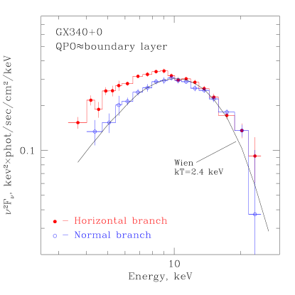
Figure 12: The absorption corrected frequency resolved spectra of QPO ($\approx$ boundary layer emission) in GX340 in the horizontal branch, Z=0–1 (lower $\dot{M}$) and upper half of the normal branch, Z=1–1.5 (higher $\dot{M}$). See Fig. 1 for specification of the regions in the color-intensity diagram. The horizontal branch data is same as in Fig. 4, 9 and 11. The solid line shows Wien spectrum with $kT=2.4$ keV.

The relatively weak dependence of the shape of the boundary layer spectrum upon the mass accretion rate (Fig. 11 and 12) and the relative constancy of the Wien temperature is somewhat surprising. It implies that in the considered range of $\dot{M}\ga 0.1\dot{M}_{\rm Edd}$ the plasma temperature at Comptonization depth in the boundary layer weakly depends upon the mass accretion rate, i.e. increase of the $\dot{M}$ does not change significantly vertical temperature structure in the boundary layer.

The fact that kHz QPO show the same behavior as other components of the aperiodic variability indicates, that they have the same origin, i.e. are caused by the variations of the luminosity of the boundary layer. Although the kHz “clock” can be in the disk or due to it’s interaction with the neutron star, the actual modulation of the X-ray flux occurs on the neutron star surface. Mendez et al. (1997) suggested similar interpretation of kHz QPO in 4U0614+09. In particular they showed, that energy spectrum of the kHz QPO can be approximately described by a blackbody spectrum with $kT\sim 1.5-1.6$ keV. Note, however, that they found different energy depedence of continuum aperiodic variability at lower frequencies. That can possibly be explained by the fact that the source was in significantly lower luminosity state, $\dot{M}\sim 10^{-2}\dot{M}_{\rm Edd}$ and it’s energy spectrum had a distinct power law component which could dominate variability at lower frequencies.

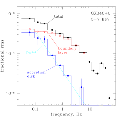
Figure 13: The power density spectra of GX340+0 in the 3–7 keV energy range (horizontal branch, same data as in Fig. 4, 9 and 11). The histogram with the error bars show power spectra of total, disk and boundary layer emission, obtained using the procedure described in the Sect. 6; the straight solid line shows a power law $P(f)=3.5e-5\times f^{-1}$. The power density is shown in units of fractional rms per Hz and all three spectra are normalized to the total count rate in the 3–7 keV band. Note, that the lower-most frequency bin is affected by the windowing effects, suppressing the power.

The disk emission is significantly less variable and does not contribute significantly to the variability of the X-ray flux at $f\ga 0.5-1$ Hz. This conclusion is in agreement with results of Churazov et al. (2001) for the high state of Cyg X-1, indicating that stability of the X-ray emission might be a common property of the optically thick accretion disk, independently on the nature of the compact object. The origin of the variable component, however, is different in the case of Cyg X-1 (and presumably in the soft state of other black hole binaries). Indeed, the spectrum of the variable component in the soft state of Cyg X-1 is identical to the time average spectrum of the hard spectral component and is adequatly represented by unsaturated Comptonization in hot ($kT_{\rm e}\sim 50-100$ keV) and optically thin ($\tau_{\rm T}\la 1$) coronal flow with possible contribution of non-thermal Comptonization. Variable component in luminous LMXBs considered in this paper, if interpreted in the framework of the Comptonization model, requires saturated Comptonizaion (Comptonization parameter $y\sim 1$) in the relatively low temperature ($kT_{\rm e}\sim 2-3$ keV) plasma and is inconsistent both qualitatively and quantitatively with the corona models usually applied to black hole binaries.

In the bright LMXB systems, the contribution of the disk variability becomes noticeable at lower frequencies, below $\sim 0.5$ Hz, where the frequency resolved spectrum changes it’s shape and becomes softer (Fig. 4 and 5; cf. results of van der Klis 1986 for GX5–1). This can be used to estimate the contribution of the disk to the observed variability of the X-ray flux. The result depends on the character of the disk variability. In order to make a crude estimate we assume that the disk variations also obey a simple linear relation described by Eq. (5):

$$F(e,t)=F_{\rm disk}(E,t)+F_{\rm BL}(E,t)\approx$$ (11)

$$\approx S_{\rm disk}(E)\times f_{\rm disk}(t)+S_{\rm BL}(E)\times f_{\rm BL}(t)$$

If disk and boundary layer variations were uncorrelated, the power density of the total signal would be:

$$P(E,\omega)\propto S_{\rm disk}(E)^{2}\times|\hat{f}_{\rm disk}(\omega)|^{2}+S_{\rm BL}(E)^{2}\times|\hat{f}_{\rm BL}(\omega)|^{2}$$

where within the accuracy of this consideration one can assume that $S_{\rm disk}(E)$ and $S_{\rm BL}(E)$ are the disk and boundary layer spectra determined in Sect. 5.3. The functions $|\hat{f}_{\rm disk}(\omega)|^{2}$ and $|\hat{f}_{\rm BL}(\omega)|^{2}$ after appropriate renormalization represent power density spectra of the disk and boundary layer and can be determined from linear fit to the square of the frequency resolved spectra in each frequency interval. The power density spectra thus computed are shown in Fig. 13 along with the total power spectrum of GX340+0 in the soft 3–7 keV energy band. The power spectrum of the accretion disk flux variations is different from that of the boundary layer, does not extend significantly to the high frequency domain, and is consistent with a power law with slope of $-1$:

$$P_{\rm disk}(f)\propto f^{-1}$$

The excess power seen at low frequencies, $F\la 0.5-1$ Hz in the soft energy band (cf. Fig. 2) can be explained as the contribution of the disk variations. At higher frequencies the variability is dominated by the boundary layer emission, giving primary contribution to quasi-periodic oscillations and the so called band limited noise compoinent (e.g. van der Klis, 1986).

7 Summary

The initial observational results are listed in Subsect. 3.3. Below we summarize the constrains on the character of the spectral variability and implications for the boundary layer and accretion disk models.

7.1 Constrains on the pattern and origin of the spectral variability in luminous LMXBs

1. Using RXTE/PCA observations of two luminous low mass X-ray binaries GX340+0 (on the horizontal/normal branch of the color-intensity diagram) and 4U1608-52 we show that the shape of the Fourier frequency resolved spectra on $\sim$ second – millisecond time scales does not depend on Fourier frequency (Fig. 4, 5 and 7).  The range of investigated timescales includes the band limited continuum noise, the kHz QPO and lower frequency QPOs observed at few tens Hz (Fig. 2, 3). Combined with the negligibly small phase lags, $\Delta\phi\la 10^{-2}$ (Fig. 6), this restricts significantly the possible pattern of spectral variability of X-ray flux and requires linear relation between flux variations at different energies (Eq. (5)).

   Considering significant difference in the expected spectra of the accretion disk and boundary layer the observed variations should be associated with either one of these two major components of the accretion flow. The X-ray variability is caused either by variations of it’s luminosity under constant spectral shape, or by small variations of a spectral parameter (e.g temperature or optical depth) – Eq. (7).

2. We compared the Fourier frequency resolved spectra with the expected spectra of the accretion disk and of the boundary layer. The predicted spectra were based on the observed energy flux/spectrum and very generic system parameters such as the source distance and neutron star spin frequency. The frequency resolved spectra are well consistent with the range of the boundary layer spectra expected for plausible range of the system parameters (Fig. 9, Table 1). On the other hand, they are significantly harder than the expected spectrum of the accretion disk. It is unlikely that the observed variations are associated with variations of the disk luminosity or spectral shape unless the disk temperature is $\sim 3-4$ kev, i.e. current accretion disk models are inapplicable to the neutron star binaries.

3. The above suggests that the major part of aperiodic and quasiperiodic variability observed in luminous LMXBs above $\sim 0.5$ Hz is caused by variations of the luminosity of the boundary layer. Its spectral shape remains nearly constant in the course of the luminosity variations. This interpretations receives additional support from the constancy of the fractional rms with energy at $E\ga 10$ keV, where expected accretion disk emission vanishes, found in case of 4U1608–52 (Fig. 10).

7.2 Implications for the models of the boundary layer and disk emission

The frequency resolved spectrum is representative of the energy spectrum of the boundary layer emission. This can be used for a more precise decomposition of the spectra of luminous LMXBs into accretion disk and boundary layer components and for quantitative comparison with predictions of the theoretical models. In the following we shall assume that boundary layer spectrum is identical to the frequency resolved spectrum, bearing in mind that this is true to certain accuracy.

1. In the considered range of the mass accretion rate $\dot{M}\sim(0.1-1)\dot{M}_{\rm Edd}$, the boundary layer spectrum in the 3–20 keV energy range depends weakly on $\dot{M}$. Its shape is remarkably similar in GX340+0 and 4U1608–52 (Fig. 11), despite the fact that the two sources have a factor of $\sim 10$ difference in the mass accretion rate (Table 2).

   In the limit of high $\dot{M}$, of the order of $\sim\dot{M}_{\rm Edd}$ (normal branch of GX340+0), the boundary layer spectrum in the 3–20 keV energy range can be adequately represented by the Wien spectrum with temperature $kT\approx 2.4$ keV (Fig. 12). At lower values of $\dot{M}$ (4U1608–52 and horizontal branch of GX340+0) the spectra are better described by Comptonization model with electron temperature of $\sim 2-4$ keV and Comptonization parameter $y\sim 1$ (Table 2). Their high energy part, $E\ga 10$ keV, is well represented by Wien spectrum with temperature of $\approx 2.1-2.3$ keV.

2. The average spectra can be adequately described by the sum of the renormalized frequency resolved spectrum and the accretion disk emission (Fig. 11). The spectrum of the latter is well described by the general relativistic accretion disk model. The other parameters, such as source distance and disk inclination angle being fixed at fudicial but plausible values, the best fit value of the mass accretion rate coincides, within a factor of $\la 1.7$ with that inferred from the observed X-ray flux and accretion efficiency appropriate for a 1.4$M_{\sun}$ neutron star with spin frequency of $\sim 500$ Hz (Table 2). This agreement is especially remarkable, given the luminosity and mass accretion rate in the two sources differ by the factor of $\sim 10$.

3. The accretion disk emission is significantly less variable than the boundary layer emission at Fourier frequencies $f\ga 0.5-1$ Hz. The power density spectrum of the disk appears to follow a power law $P_{\rm disk}(f)\propto f^{-1}$ and contributes to the overall variability in the soft energy band and in the low frequency domain only (Fig. 13).

4. The kHz QPOs apear to have the same origin as aperiodic and quasiperiodic variability at lower frequencies. The msec flux modulations originate on the surface of the neutron star although the kHz “clock” might reside in the disk or be determined by the disk – neutron star interaction.

5. Finally we point out that in the case of GX340+0 and presumably other Z–sources, the above results apply to the normal and horizontal branches of the color-intensity diagram. The source behaviour on the flaring branch, believed to correspond to super-Eddington accretion is more complex and is beyond the scope of this paper.