A Taylor-Couette Dynamo

Recent experiments have shown that it is possible to study a fundamental astrophysical process such as dynamo action in controlled laboratory conditions using simple MHD flows. In this paper we explore the possibility that Taylor-Couette flow, already proposed as a model of the magneto-rotational instability of accretion discs, can sustain generation of magnetic field. Firstly, by solving the kinematic dynamo problem, we identify the region of parameter space where the magnetic field’s growth rate is higher. Secondly, by solving simultaneously the coupled nonlinear equations which govern velocity field and magnetic field, we find a self-consistent nonlinearly saturated dynamo.

1 Motivation

Even though astrophysical objects possessing observable magnetic fields are extremely diverse, it is widely accepted that the physical mechanisms supporting the fields are fairly universal and rely on features common to virtually all astrophysical objects (e.g. differential rotation, convective or turbulent motions, etc.). MHD dynamo theory quantifies this idea and states that astrophysical magnetic fields are created by inductive currents driven by motions of electrically conducting plasmas (Moffatt 1978). Until recently, dynamo action was the subject of theoretical or numerical investigations only. The recent demonstration of dynamo action in controlled laboratory experiments (Gailitis et al. 2001; Stieglitz & Muller 2001) has stimulated interest in the study of dynamo action in confined geometries of potential laboratory interest, such as spheres or cylinders. The configuration of an MHD fluid confined between concentric cylinders (Taylor-Couette flow) is particularly relevant. Dynamo action is associated with spiral and sheared flows, which suggests that Taylor-vortex flow is good candidate for dynamo experiments in a simple geometry.

At the same time, Taylor-Couette flow is already a useful benchmark for studying instabilities relevant to astrophysical processes (Balbus & Hawley 1991; Ji et al. 2001; Rüdiger & Zhang 2001), as the flow pattern can model Keplerian motion. In particular we note the works of Dobler et al. (2002) who studied the dynamo mechanism in the presence of an imposed axial flow (resulting in a screw dynamo) and of Laure et al. (2000) who concentrated on the basic Taylor-Couette configuration. The latter performed a kinematic dynamo calculation in this geometry and demonstrated that an imposed Taylor-vortex flow is capable of dynamo action. The combination of shear with simple roll flows has also been modelled by Dudley & James (1989) in spherical geometry. There it was demonstrated that magnetic field generation is sensitive to the nature of the driving flow. Our work differs from the studies of Dudley & James (1989) and Laure et al. (2000) in two important respects: first (kinematic dynamo) we use the velocity fields that are actual solutions of the Navier-Stokes equations to generate a magnetic field, not arbitrary imposed flow fields; secondly (fully self-consistent dynamos) we let these velocity fields evolve alongside the magnetic field, thus solving the full MHD equations.

The aim of this work is two-fold. Firstly we widen the study of Laure et al. (2000) in the parameter space by finding the growth of the magnetic field as a function of the flow patterns. Secondly, and more importantly, we go beyond the limits of (linear) kinematic theory and investigate the fully self-consistent dynamo mechanism (magnetic fields and flow pattern affect each other and saturate nonlinearly).

2 Model

We consider an incompressible fluid contained between two coaxial cylinders of inner radius $R_{1}$ and outer radius $R_{2}$ which rotate at prescribed angular velocities $\Omega_{1}$ and $\Omega_{2}$. The velocity and magnetic fields, $\@vec{V}(r,\theta,z,t)$ and $\@vec{B}(r,\theta,z,t)$ are determined by the MHD equations which we write in dimensionless form as

$$\frac{\partial\@vec{V}}{\partial t}+(\@vec{V}\cdot\mbox{\boldmath$\nabla$})\@vec{V}=-\mbox{\boldmath$\nabla$}p+\nabla^{2}\@vec{V}+(\mbox{\boldmath$\nabla$}\wedge\@vec{B})\wedge\@vec{B},$$ (1)

$$\frac{\partial\@vec{B}}{\partial t}=\frac{1}{P_{m}}\nabla^{2}\@vec{B}+\mbox{\boldmath$\nabla$}\wedge(\@vec{V}\wedge\@vec{B}),$$ (2)

$$\mbox{\boldmath$\nabla$}\cdot\@vec{B}=0,\quad\mbox{\boldmath$\nabla$}\cdot\@vec{V}=0,$$ (3)

where $p$ is the pressure. In writing (1) and (2) we used $\delta=R_{2}-R_{1}$ as unit of length, $\delta^{2}/\nu$ as unit of time and $(\mu_{0}\rho)^{\frac{1}{2}}\nu/\delta$ as unit of magnetic field, where the kinematic viscosity $\nu$, the density $\rho$ and the permeability $\mu_{0}$ are constant. The governing dimensionless parameters of the system are the Reynolds numbers $\mbox{\it Re}_{1}$, $\mbox{\it Re}_{2}$, the radius ratio $\eta$, and rotation ratio $\mu$,

$$\mbox{\it Re}_{1}=\frac{R_{1}\Omega_{1}\delta}{\nu},\quad\mbox{\it Re}_{2}=\frac{R_{2}\Omega_{2}\delta}{\nu},\quad\eta=\frac{R_{1}}{R_{2}},\quad\mu=\frac{\Omega_{2}}{\Omega_{1}},$$ (4)

together with the magnetic Prandtl number $P_{m}$,

$$P_{m}=\frac{\nu}{\lambda},$$ (5)

where $\lambda=1/(\mu_{0}\sigma)$ is the magnetic diffusivity and $\sigma$ is the electrical conductivity.

We assume no-slip boundary conditions for $\@vec{V}$, and electrically insulating boundary conditions for $\@vec{B}$. For modes of the form $\@vec{B}(r,t,z)=\@vec{B}(r)\,{\mathrm{e}}^{{\mathrm{i}}(\alpha z+m\theta)}$ these conditions are

$$\begin{array}[]{rl}\alpha=m=0:&B_{\theta}=B_{z}=0;\\[2.0pt] \alpha=0,\,m\neq 0:&\partial_{\theta}B_{r}=\pm mB_{\theta},\quad B_{z}=0;\\[2.0pt] \alpha\neq 0:&{\displaystyle\partial_{z}B_{r}=\frac{\partial_{r}{\mathcal{B}}_{m}}{{\mathcal{B}}_{m}}\,B_{z},\quad\frac{1}{r}\,\partial_{\theta}B_{z}=\partial_{z}B_{\theta},}\end{array}$$ (6)

where for $\pm$ we take $+$ at $R_{1}$, $-$ at $R_{2}$. The symbol ${\mathcal{B}}_{m}(r)$ indicates the modified Bessel functions, $I_{m}(\alpha r)$ at $R_{1}$ and $K_{m}(\alpha r)$ at $R_{2}$. The axial wavelength of a pair of Taylor-vortices is $2\pi/\alpha$.

Our numerical method for timestepping the 3D nonlinear MHD equations is detailed in Willis & Barenghi (2002). The formulation is based on representing $\@vec{V}$ and $\@vec{B}$ with the toroidal-poloidal decomposition

$$\@vec{A}=\psi_{0}\,{{\hat{\@vec{\theta}\mkern 3.0mu}\mkern-3.0mu}{}}+\phi_{0}\,{{\hat{\@vec{z}\mkern 3.0mu}\mkern-3.0mu}{}}+\mbox{\boldmath$\nabla$}\wedge(\psi\@vec{r})+\mbox{\boldmath$\nabla$}\wedge\mbox{\boldmath$\nabla$}\wedge(\phi\@vec{r}),$$ (7)

where $\psi(r,t,z)$, $\phi(r,t,z)$ and $\psi_{0}(r)$, $\phi_{0}(r)$ contain the periodic and non-periodic parts of the field respectively. The potentials are expanded spectrally over Fourier modes in the azimuthal and axial directions and over Chebyshev polynomials in the radial direction.

The governing equations for the magnetic field are the $r$-components of the induction equation and its first curl. For the velocity we follow the procedure applied to the magnetic field and take the $r$-components of the momentum equation and its first curl. As the pressure has not been eliminated, we also take the divergence to obtain the pressure–Poisson equation. All five governing equations are second order in $r$. Time stepping is based on a combination of second order accurate Crank-Nicolson and Adams-Bashforth methods. The code has been tested against published results with and without a magnetic field (Chandrasekhar 1961; Roberts 1964; Marcus 1984; Jones 1985; Barenghi 1991).

3 Kinematic dynamo

For prescribed Reynolds number $\mbox{\it Re}_{1}$, wavenumber $\alpha$, rotation ratio $\mu$ and radius ratio $\eta$ the Navier-Stokes Eq. (1) is solved in the absence of a magnetic field. We always assume $\mbox{\it Re}_{1}>\mbox{\it Re}_{1c}$, where $\mbox{\it Re}_{1c}$ is the critical Reynolds number at which azimuthal Couette flow is unstable to the formation of axisymmetric Taylor vortices (Chandrasekhar 1961). We also assume $\alpha=3.14$, which corresponds to almost square cells. The nonlinear Taylor-vortex flow $\@vec{V}$ thus obtained is used when solving the induction Eq. (2) for $\@vec{B}$, starting from a small magnetic seed field of wavelength $\alpha_{B}$.

Note that $\@vec{V}$ being fixed, (2) is linear and has eigenfunction solutions $\@vec{B}$ which grow or decay exponentially. If the real part of the growth rate $\sigma_{B}\hskip 1.2pt$ is positive then the magnetic field grows (kinematic dynamo action). Following Laure et al. (2000) we assume $\alpha_{B}=\frac{1}{2}\alpha$, the characteristic length for the magnetic field is the length of two pairs of Taylor-vortices. In several calculations with $\alpha_{B}=\alpha$ we found the magnetic seed field decayed quickly.

Figure 1: Growth rates $\sigma_{B}\hskip 1.2pt$ for various $\eta$ and $m$, where $\mbox{\it Re}_{1}=2\mbox{\it Re}_{1c}(\eta)$, $P_{m}=2$.

The axisymmetric flow cannot generate an $m=0$ magnetic field. In Fig. 1 we see that in narrower gaps the dynamo prefers larger $m$. The dynamo is local here in the sense that the characteristic length scale for the magnetic field comply with the scale of the flow. As the Taylor-vortex flow is itself unstable to non-axisymmetric perturbations in narrower gaps (see Jones 1985), we usually consider the case $\eta=0.5$ where $m=1$ is preferred. The relative stability of Taylor-vortex flow in wider gaps also allows for a clearer interpretation of the affect of the magnetic field in the nonlinear self-consistent solutions presented in Sect. 4.

Figure 2: Growth rates $\sigma_{B}\hskip 1.2pt$ for various $\eta$ as a function of $P_{m}$, where $\mbox{\it Re}_{1}=2\mbox{\it Re}_{1c}(\eta)$, $m=1$. Critical Reynolds numbers at $\eta=0.3,0.5,0.7,0.9$ are respectively $\mbox{\it Re}_{1c}=73.3,68.2,79.5,131.6$.

Figure 2 shows that, not surprisingly, $\sigma_{B}\hskip 1.2pt$ falls off sharply when $P_{m}<1$, in which case much larger Reynolds numbers (relative to $\mbox{\it Re}_{1c}$) are needed for dynamo action. Generally it is easier to generate a magnetic field in media with larger magnetic Prandtl numbers. This is believed to be the case for warm weakly ionised gas, McIvor (1977), Kulsrud & Anderson (1992).

Figure 3: Growth rates $\sigma_{B}\hskip 1.2pt$ as versus $\mbox{\it Re}_{1}$ at $\eta=0.5$.

Figure 3 shows growth rates as a function of $\mbox{\it Re}_{1}$ with $\mbox{\it Re}_{2}=0$, $\eta=0.5$ for a few values of $P_{m}$. Driving the flow harder seems to move the flow into a regime which is less favourable for magnetic field generation when the outer cylinder is fixed. Allowing co-rotation, the stability boundary for onset of Taylor-vortex flow tends to the Rayleigh line $\mu=\eta^{2}$ for large Reynolds numbers. As circular-Couette flow $\Omega(r)=a+b/r^{2}$ alone is not capable of dynamo action, we must consider flows which are Rayleigh unstable, $\mu<\eta^{2}$.

Figure 4: Growth rates $\sigma_{B}\hskip 1.2pt$ with co-rotation. $\eta=0.5$, $P_{m}=2$. At $\mu=0,\,\frac{1}{2}\eta^{2},\,\frac{3}{4}\eta^{2},\,\frac{7}{8}\eta^{2}$, critical Reynolds numbers are $\mbox{\it Re}_{1c}=68.2,84.3,112.7,155.3$ respectively.

Figure 4 shows growth rates as a function of $\mbox{\it Re}_{1}$ for different values of $\mu$. Again, we normalise the intensity of the drive $\mbox{\it Re}_{1}$ by the critical value $\mbox{\it Re}_{1c}$. It is apparent that magnetic field generation is easier with co-rotating cylinders and $\mu=\frac{3}{4}\eta^{2}$ is an important case. At this particular $\mu$ the amplitude of the azimuthal disturbance $V^{\prime}_{\theta}=V_{\theta}-r\,\Omega(r)$ and $V_{z}$ are similar, seen in Fig. 5.

Figure 5: Amplitude of the azimuthal disturbance $V^{\prime}_{\theta}=V_{\theta}-r\,\Omega(r)$ drops as $\mu\to\eta^{2}$ in the absence of a magnetic field. At each $\mbox{\it Re}_{1}/\mbox{\it Re}_{1c}$ the amplitudes of $V_{z}$ are close for all $\mu$.

At a given $\mbox{\it Re}_{1}/\mbox{\it Re}_{1c}(\mu)$, the components $V_{r}$, $V_{z}$ appear to be very similar in structure and amplitude. However, $V_{\theta}$ changes significantly with $\mu$.

Figure 6: Dependence on $P_{m}$ for the driving required for field generation. $\mu=\frac{3}{4}\eta^{2}$, $\eta=0.5$.

Of the rotation ratios considered in Fig. 4, $\mu=\frac{3}{4}\eta^{2}$ would appear to be most favourable for magnetic field generation. We define $\mbox{\it Re}_{1}^{*}$ as the critical Reynolds number at which $\sigma_{B}\hskip 1.2pt=0$ (marginal state for the onset of dynamo action) for this $\mu$. Figure 6 shows how $\mbox{\it Re}_{1}^{*}$ depends on $P_{m}$. Fitting the last three points for small $P_{m}$ we obtain the slope $-1.1$. Approximately, $\mbox{\it Re}_{1}^{*}/\mbox{\it Re}_{1c}\propto 1/P_{m}$, for small $P_{m}$. Our interest in this case is linked to the small magnetic Prandtl numbers of laboratory fluids. Defining the magnetic Reynolds number $\mbox{\it Re}_{m}$ as

$$\mbox{\it Re}_{m}=\frac{R_{1}\,\Omega_{1}\,\delta}{\lambda}=\mbox{\it Re}_{1}\,P_{m}$$ (8)

we conclude that the critical magnetic Reynolds number $\mbox{\it Re}_{m}^{*}=\mbox{\it Re}_{1}^{*}\,P_{m}$ is approximately constant and ${\mathcal{O}}(10^{2})$ for suitably chosen $\eta$, $\mu$. Here $\mu\approx\frac{3}{4}\eta^{2}$ but the most suitable $\mu$ is likely to vary for other $\eta$. The $\mbox{\it Re}_{m}^{*}$ above are also consistent with the results of Laure et al. (2000) who found $\mbox{\it Re}_{m}^{*}={\mathcal{O}}(10^{2})$ in their calculations with $\mu=0$.

4 Self-consistent dynamo

In this section Eqs. (1) and (2) are solved simultaneously using as initial conditions the previously prescribed Taylor-vortex flow $\@vec{V}$ and the accompanying eigenfunction $\@vec{B}$.

Figure 7: Magnetic energy versus time as the magnetic field saturates. $\eta=0.5$, $P_{m}=2$. (a) $\mu=0$, $\mbox{\it Re}_{1}=1.5\mbox{\it Re}_{1c}$, $E_{\mbox{\it\scriptsize CCF}}=4.15\times 10^{4}$. (b) $\mu=\frac{3}{4}\eta^{2}$, $\mbox{\it Re}_{1}=2\mbox{\it Re}_{1c}$, $E_{\mbox{\it\scriptsize CCF}}=3.63\times 10^{5}$.

Figure 7 shows that after an initial transient the magnetic energy $E_{B}$ saturates to a constant value, indicating dynamo action. At the parameters in Fig. 7 the calculations required 16 Chebyshev modes radially, 16 axial and 12 azimuthal Fourier modes with a timestep of $10^{-4}\tau$, where $\tau$ is the rotation period of the inner cylinder. The magnetic energy is plotted as a fraction of the energy of the driving circular-Couette flow $E_{\mbox{\it\scriptsize CCF}}$, the energy source for the dynamo. The energy sink is an increased viscous dissipation in the velocity disturbance in addition to Ohmic dissipation. In these calculations the dynamo is dynamically self consistent ($\@vec{V}$ and $\@vec{B}$ evolve together).

Figures 8 and 9 show the typical field structure of the initial conditions.

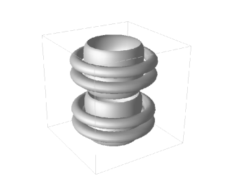
Figure 8: Isosurface of helicity $|\@vec{V}\cdot\mbox{\boldmath$\nabla$}\wedge\@vec{V}|$ at $\eta=0.5$, $\mbox{\it Re}_{1}=1.5\mbox{\it Re}_{1c}$, $\mu=0$. Shown over two axial periods.

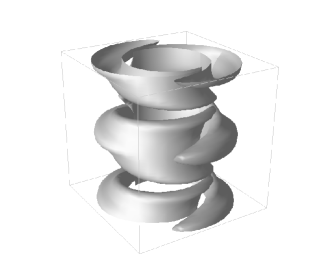
Figure 9: Isosurface of $|\@vec{B}|$. The field is $m=1$. Same parameters as Fig. 8 with $P_{m}=2$ (as in Fig. 7a).

A fixed outer cylinder was taken for visualisation purposes as the surfaces are less self-obscuring. The initial flow pattern $\@vec{V}$ has $m=0$ symmetry and as $\mbox{\it Re}_{1}>\mbox{\it Re}_{1c}$ vortex cores are slightly shifted towards the outflow regions. The eigenfunction $\@vec{B}$ in Fig. 9 has $m=1$ symmetry. The flow pattern, initially axisymmetric is deformed by the action of the Lorentz force $(\mbox{\boldmath$\nabla$}\wedge\@vec{B})\wedge\@vec{B}$ and acquires an $m=2$ contribution visible in Fig. 10.

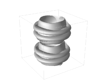
Figure 10: Isosurface of helicity at magnetic field saturation. The flow is $m=2$, looking the same if rotated by $180^{\circ}$. Parameters as in Fig. 7a.

Figure 11: Kinetic energy of the velocity disturbance and the magnetic energy of the various azimuthal modes. Parameters as in Fig. 7a.

Figure 11 shows the kinetic energy of the velocity disturbance and the magnetic energy of the various azimuthal modes, $E(m)$ and $E_{B}(m)$ respectively, for the saturated dynamo of Fig. 7a. The velocity has contributions $m=0,2,4,\dots$ and the magnetic field has $m=1,3,5,\dots$ etc. The perturbation to the magnetic field is difficult to appreciate visually on the dominant $m=1$ structure. It remains rather similar to Fig. 9.

5 Discussion

By solving the kinematic dynamo problem, we have determined that a Taylor-vortex flow pattern can sustain a growing magnetic field.

Like in the models of Dudley & James (1989) we also find that the dynamo is sensitive to the flow pattern. Further, for flows that are capable dynamo action we see that the growth rate is not a monotonic increasing function of the Reynolds number. This is not seen in Dudley & James (1989), most likely due to the prescribed form for the driving flow patterns.

In the Taylor-vortex flow the best growth rates have been obtained with co-rotation. The relative magnitude of the shear and roll in the flow plays an important part in the success of the dynamo mechanism.

Solving the full MHD equations we have demonstrated the existence of a fully self-consistent nonlinearly saturated dynamo. Hopefully these results will stimulate experimental work on the problem. Future theoretical work will investigate dynamo action in hydrodynamically stable flows and address the nature of the magnetic field structure when the dynamo is driven harder – our dynamo is laminar. Most of the present work is concerned with wider gaps.

References

- Balbus & Hawley (1991) Balbus, S. A. & Hawley, J. F. 1991, ApJ, 376, 214.
- Barenghi (1991) Barenghi, C. F. 1991, J. Comput. Phys. 95, 175
- Chandrasekhar (1961) Chandrasekhar, S. 1961, Hydrodynamic and Hydromagnetic Stability (Oxford).
- Dobler et al. (2002) Dobler, W., Shukurov, A. & Brandenburg, A. 2002, Phys. Rev. E 65 art. no. 036311.
- Dudley & James (1989) Dudley, M. L. & James, R. W. 1989, Proc. R. Soc. Lond. A 425, 407-429.
- Gailitis et al. (2001) Gailitis, A., Lielausis, O., Platacis, E. et al., Phys. Rev. Lett. 86, 3024-3027.
- Ji et al. (2001) Ji, H., Goodman, J. & Kageyama, A. 2001, MNRAS, 325, L1-L5.
- Jones (1985) Jones, C. A. 1985, J. Fluid Mech. 157, 135.
- Kulsrud & Anderson (1992) Kulsrud, R. M. & Anderson, S. W. 1992, ApJ, 396, 606.
- Laure et al. (2000) Laure, P., Chossat, P. & Daviaud, F. 2000 In Dynamo and dynamics, a mathematical challenge. Nato science series II, 26, pp. 17-24
- Marcus (1984) Marcus, P. S. 1984, J. Fluid Mech., 146, 45.
- McIvor (1977) McIvor, I. 1977, MNRAS 178, 85-99.
- Moffatt (1978) Moffatt, H. K. 1978, Magnetic field generation in electrically conducting fluids (Cambridge).
- Roberts (1964) Roberts, P. H. 1964, Proc. Cam. Phil. Soc. 60, 635.
- Rüdiger & Zhang (2001) Rüdiger, G. & Zhang, Y. 2001 A&A, 378, 302.
- (16) Steiglitz, R. & Müller, U. 2001 Phys. Fluids 13, 561-564.
- Willis & Barenghi (2002) Willis, A. P. & Barenghi, C. F. 2002, to appear in J. Fluid Mech.