More on the determination of the coronal heating function from Yohkoh data

Abstract

Two recent works have analyzed a solar large and steady coronal loop observed with Yohkoh/SXT in two filter passbands to infer the distribution of the heating along it. Priest et al. (2000) modelled the distribution of the temperature obtained from filter ratio method with an analytical approach, and concluded that the heating was uniform along the loop. Aschwanden (2001) found that a uniform heating led to an unreasonably large plasma column depth along the line of sight, and, using a two component loop model, that a footpoint-heated model loop (with a minor cool component) yields more acceptable physical solutions. We revisit the analysis of the same loop system, considering conventional hydrostatic single loop models with uniformly distributed heating, and with heating localized at the footpoints and at the apex, and an unstructured background contribution extrapolated from the region below the analyzed loop. The flux profiles synthesized from the loop models have been compared in detail with those observed in both filter passbands with and without background subtraction; we find that background-subtracted data are fitted with acceptable statistical significance by a model of relatively hot loop ($\sim 3.7$ MK) heated at the apex, with a column depth $\sim 1/10$ of the loop length. In discussing our results, we put warnings on the importance of aspects of data analysis and modeling, such as considering diffuse background emission in complex loop regions.

1 Introduction

The most recent solar X-ray and UV missions (Yohkoh, SoHO, TRACE) have produced a significant amount of spectacular data and images of the corona. The improved spatial resolution and sensitivity of the detectors have revealed the highly structured and variable nature of the corona and have stimulated the interest of solar physics community.

Whereas the morphological interpretation of the images is often straightforward and has highlighted the presence of a variety of new structures and phenomena, the physical interpretation of the data and the inference of indications about items such as the heating of the corona is a much more delicate matter. A possible problem is that many physical and instrumental effects act concurrently and non-linearly. The coronal plasma is highly thermally conductive along the magnetic field lines but much less across them. As a result, non-uniform and localized heating sources which ignite coronal loops will at the same time be elusive, because the temperature increases rapidly along the whole loop, and determine a significant thermal stratification across the loop and along the line of sight. Since the coronal plasma is mostly optically thin, a telescope observing a loop will then collect the emission from multiple thermal components along the line of sight, filter them with different weights, depending on its passband, and sum them up to yield a single data number for each image pixel. The reconstruction of the original thermal structure of the plasma column in a pixel is a difficult task and some attempts have been made possible by multi-line observations with SoHO (Schmelz et al. 2001). When analyzing data from wide-band imaging instruments such as Yohkoh/SXT, one approach is to obtain maps of the weighted average temperature of the various thermal components along the line of sight. The interpretation of temperature distributions is somewhat easier along bright loop structures, because there one has the reasonable expectation that one thermal plasma component has a much larger emission measure than the others, and therefore dominates the emission and can be determined reliably.

This vision has driven recent studies of the thermal structure along coronal loops, and of its usage as indicator of the distribution of the heating deposition within the loop (Priest et al. 2000, Aschwanden 2001). The concept of these works was to compare the temperature distributions of bright coronal loops derived from the data with those obtained from models of thermally structured single coronal loops (or combinations of them). Priest et al. (2000) used an analytical approach and devised a method to infer the heating distribution along the loops from the analysis of temperature profiles, showing that along several bright steady-state large-scale loops observed at the solar limb the temperature distribution indicates uniformly distributed heating. Aschwanden (2001) revisited the analysis of one of the loops selected by Priest et al. (2000), and found that the previous approach led to inconsistent results and, in particular, to an unreasonably large plasma column depth required to match the emission measure inferred from the data. Using a two component loop model to explain the observations, he also found that the data are consistently fitted instead by a model coronal loop with a heating highly localized at the footpoints and with a cool background component.

In this work we present a further analysis of the same loop system, motivated as follows. The selected loop system is relatively bright, well outstanding at the solar limb. We might then suppose relatively large emission measure, high plasma pressure, and assuming that it is a steady structure, we can also infer, according to loop scaling laws (Rosner et al. 1978), high temperature at their apex, maybe higher than $\sim 2$ MK, which is the temperature obtained from the previous data analyses. On the other hand, neither previous analyses include, or include only partially, a component which instead may be important: “the loop system is embedded in a hazy background” (Aschwanden 2001). This background is significant, especially in the region of the loop apex, where the loop signal is fainter than elsewhere, due to the plasma gravitational stratification. One possible hypothesis, that we pursue here, is that the haze may be the effect of the presence of many other disordered faint loops, or of a streamer, which extend over the whole loop system and intersect the analysed structure along the line of sight. Such background may not be described as a simple hydrostatic equilibrium, and deserves proper attention, since it may affect systematically the filter ratio and temperature values. Another item stimulating our analysis is the finding by Aschwanden (2001) of a solution with a very small scaling height of the heating and temperature maxima at the loop footpoints, quite a puzzling result in the light of previous well-established loop modeling (Rosner et al. 1978, Serio et al. 1981).

Here we revisit the loop system, describing the main loop component with conventional hydrostatic single loop models and deriving the background component directly from the data. We compare the brightness profiles observed along the loop in the two SXT filter passbands with and without background subtraction to those obtained from the loop models. The modeling explores three different scenarios of heating deposition: uniform distribution, localized at the footpoints and localized at the apex, i.e. a more complete sampling than in Aschwanden (2001). The model results are compared to data with detailed fitting procedures, and attention is paid to the values of column depth obtained to match the observed fluxes. Section 2 describes the analysis of the data and their comparison with loop models; Sect. 3 discusses the results and their implications.

2 Data Analysis and Modeling

2.1 The Data

The loop system was observed with Yohkoh/SXT on 3 October 1992. The data consist of a sequence of full-disk 512$\times$512 pixel images ($\approx 5$” pixel side), basically in the Al.1 and Al/Mg/Mn filter passbands, taken with various exposure times during the whole day. The data have been preliminarily processed with the standard Yohkoh data analysis system (SXT_PREP).

We have checked that the loop to be analyzed remains quite stable and stationary during the whole day. In order to enhance the signal-to-noise ratio, we then average the long-exposure (2.7 s and 15 s) images over the whole day (as done in Aschwanden 2001, 57 images in the Al.1 filter and 55 images in the Al/Mg/Mn filter). Fig. More on the determination of the coronal heating function from Yohkoh data shows the resulting image in the Al.1 filter passband. We extract the loop flux profiles within the arch-like strip (14 pixels wide) outlined in the figure. The strip has been divided into 31 sectors with approximately equal area. The flux profiles are then the sequences of Data Numbers averaged over each sector along the loop. DN fluctuations from each image to the other have been taken as the main source of data uncertainty.

As remarked by Aschwanden (2001), the loop system is embedded in a ”hazy” background. Here we make the hypothesis that this background is mostly due to the presence of other disordered faint loops and/or of a streamer which extend over the whole loop system and intersect the loop along the line of sight. Since the brightness of the haze is comparable to the loop brightness in the upper loop region, the effect of the background may be significant in the analysis and modeling of the loop emission. Some enhancement of the data quality was achieved by Priest et al. (2000) by reducing the radiation scattering due to SXT wings (Foley 1998), but, as we have checked (using the procedure SXT_SCATTER), the amount of scattering ($\leq 20$ %) cannot account for the high background.

In the hypothesis that the background emission includes disorganized contributions from other faint structures, our approach has been to evaluate it with a model-independent procedure and to subtract it from the emission measured along the loop. To evaluate the background, we measure the emission in a region below the main visible arcade, where the emission is relatively faint, unstructured and as far as possible free of small evident loops. We then assume that, in the loop region, the background is stratified in the radial direction from the Sun center, and extends to involve the whole loop system. We extract the background fluxes (one for each filter) along the rectilinear strip (ten pixels wide) outlined in Fig. More on the determination of the coronal heating function from Yohkoh data, roughly perpendicular to the disk limb. This strip is chosen to have a signal decreasing upwards as far as possible smoothly. The resulting radial background profiles are then subtracted from the respective loop flux profiles, as a function of the distance of the loop sectors from the limb. One of the background profiles is shown in Fig. More on the determination of the coronal heating function from Yohkoh data, described below. The background flux results to be negligible nowhere along the loop, being of the order of 50% of the total flux. This procedure also allows us to limit the number of free parameters in fitting the dominant loop structure, which is the main target of the analysis.

We extract the loop flux within the arch-like strip shown in Fig. More on the determination of the coronal heating function from Yohkoh data which follows the geometry of the loop system. The loop enclosed in the strip does not appear to be perfectly semicircular, and symmetric around an axis perpendicular to the limb. We have assumed this to be due to a projection effect: the loop may not lie on a plane perpendicular to the line of sight. Then we have considered the data along half of the loop (the right leg) and corrected the coordinates along the loop for the projection effect (assuming a rotation around the symmetry axis only). As shown by the modeling results below, this allows us to make detailed comparisons with semicircular symmetric loop models.

2.2 Modeling

As done in Priest et al. (2000) and Aschwanden (2001), we try to compare the loop data with hydrostatic loop models. Priest et al. (2000) compare temperature values derived from the data with those predicted by models. Temperature values are obtained from the data with the filter ratio method, i.e. using the ratio of the flux in two filter passbands. The temperature values are then affected by two sources of uncertainties (one for each filter Data Number) and by the presence of high background. Instead of using temperature, our approach is then to compare flux profiles synthesized from model results directly to observed flux profiles corrected for background subtraction. The diagnostics on plasma temperature will then descend from the parameters of the model (or models) which is (are) found to provide a good description of the data.

The loop system is stable and steady on a time scale ($\sim 1$ day) much longer than the relevant physical time scales, i.e. the sound crossing time and the cooling times ($\lesssim$ few hours). We then consider standard hydrostatic single loop models as in Serio et al. (1981), semicircular, with constant cross-section along the loop and symmetric with respect to the loop apex. Given the extension of the loop system, gravity cannot be ignored and the loop is assumed to be perpendicular to the solar surface. The loop half-length is set to L = 380 Mm as in Aschwanden (2001). The model is based on the equations of plasma hydrostatic equilibrium and of energy balance among radiative losses, a phenomenological term of local heat input in the plasma and thermal conduction according to Spitzer’s formulation. The lower boundary of the loop is set at $2\times 10^{4}$ K, and there we assign the base pressure and the conduction flux ($F_{C}\sim 0$).

We generate models with various loop base pressures, corresponding to loop apex temperature logarithmically spaced (with step $\sim 0.05$) in the range 1 – 10 MK, for three different distributions of the heating along the loop: uniform heating, heating localized at the footpoints, and heating localized at the loop apex. The heating at the footpoints is described with a heating distribution exponentially decreasing upwards from the loop base, with a scale height $s_{H}=127$ Mm, i.e. 1/3 the loop half length. With this heating distribution we explore solutions for loop maximum temperatures below $\sim 5$ MK. We do not consider models with significantly smaller heating scale heights: they lead to loops with temperature maximum localized in the region of the loop footpoints. Such loops have been shown to be unstable (Rosner et al. 1978, Serio et al. 1981), and therefore unlikely to describe the loop analyzed here, which appear to be steady for a time of the order of a whole day. For the cases of heating at the apex, we assume a Gaussian distribution centered at the apex, with width $\sigma_{H}=10$ Mm.

Table 1: Parameters of loop models

					Al.1		AlMgMn
N.	Modela	$P_{0}^{b}$	$T_{max}^{c}$	$H_{0}^{d}$	Col.Dep.e	$\chi^{2}_{\nu}$	Col.Dep.e	$\chi^{2}_{\nu}$	Shift
		dyne cm-2	MK	$10^{-3}$ erg cm-3 s-1	pix		pix		pix
Unsubtracted data - Uniform heating
1	L	0.13	2.3	0.007	820	370	830	240	0
2	B	0.38	3.3	0.025	17	65	16	31	0
3	H	1.5	5.3	0.14	0.51	260	0.43	110	0
Unsubtracted data - Base heating
4	L	0.09	1.7	0.014	3800	4300	5000	1500	0
5	B	0.19	2.2	0.033	300	21	310	30	0
6	H	0.53	3.1	0.12	7.0	120	6.4	47	0
Unsubtracted data - Top heating
7	L	0.07	2.2	0.09	20000	4600	25000	1500	-6
8	B	0.15	2.9	0.23	740	230	730	88	-6
9	H	0.7	4.9	1.5	4.9	780	4.4	340	-6
Bkg-subtracted - Uniform heating
10	L	0.09	2.0	0.004	1300	15	1600	31	0
11	H	0.38	3.3	0.025	6.5	24	6.3	78	0
12	B	3.0	6.7	0.33	0.05	11	0.04	19	0
Bkg-subtracted - Base heating
13	L	0.09	1.7	0.014	1700	47	2100	100	0
14	B	0.13	1.9	0.021	500	5.0	570	7.8	0
15	H	0.53	3.1	0.12	2.7	13	2.6	31	0
Bkg-subtracted - Top heating
16	L	0.07	2.2	0.09	8500	53	10000	130	-6
17	B	0.30	3.7	0.5	22	0.50	20	1.7	-6
18	H	3.0	8.3	9.6	0.09	2.8	0.07	8.1	-6

^a - Label of the model as in Fig. More on the determination of the coronal heating function from Yohkoh data, B, L and H indicate ”Best fit model”, ”Lower temperature model” and ”Higher temperature model”, respectively.
^b - Pressure at the loop footpoints
^c - Maximum loop temperature
^d - Maximum heating rate per unit volume
^e - Column depth obtained from normalization of the emission synthesized from the loop models to best-fit the data.

From the temperature and density profiles obtained from the models we synthesize the loop emission filtered through the two SXT filter passbands, with the same procedure as in Aschwanden (2001). We then perform a best-fit procedure to the data along half of the loop, by finding analytically the normalization factor which minimizes the $\chi^{2}$ of each model to the data points. This normalization factor is the only parameter of the fitting and represents the plasma column depth of the loop system along the line of sight. We then look for the models yielding the lowest $\chi^{2}$ values among the models with different maximum temperatures and the same heating distribution, and then for the best-fit model among those with different heating distributions. This procedure is repeated on the data, both with and without background subtraction. In order to make the fitting in some way independent of possible errors in the determination of the loop length and of the real position of the relevant footpoint (see also the problem of submerged footpoints presented in McKay et al. 2000), the first three data points from the left are excluded from the $\chi^{2}$ calculation, and we repeat the fitting for two different values of the relative shift of the model to the data, one assuming the model loop footpoint coincident with the data origin, and the other shifted backwards by $2\times 10^{9}$ cm. In the following we will show results only for the value of the shift yielding the better $\chi^{2}$ value. We cannot exclude also some effects on the results due to loop opening at the base the loop. These are not expected to be important in corona (Serio et al. 1981), and may somewhat influence the normalization factor (Aschwanden 2001), but warnings on this have been raised due to the possibility that the coronal footpoint of a loop may have any base temperature since it may virtually be thermally isolated from the chromosphere (Dowdy et al. 1985).

Table 1 and Figs. More on the determination of the coronal heating function from Yohkoh data and  More on the determination of the coronal heating function from Yohkoh data show some relevant results of the modeling, separating the cases of data without (hereafter unsubtracted data) and with background subtraction, and of models with uniform, base and top heating. Table 1 shows the significant parameters of the models in Figs. More on the determination of the coronal heating function from Yohkoh data and  More on the determination of the coronal heating function from Yohkoh data, and in particular the pressure at the base of the model loop, its maximum temperature (at the top of the model loop), the (maximum) heating rate per unit volume, the loop plasma column depth derived as normalization factor, the reduced $\chi^{2}$ values (11 d.o.f.), respectively obtained for the two filters, and the shift value yielding the best $\chi^{2}$.

In Fig. More on the determination of the coronal heating function from Yohkoh data, each panel shows the data (data points) in both filters, the best-fitting model (solid lines) and other two models, one with lower and one with higher maximum temperature, for comparison. The origin of the reference system is at the loop footpoint. The panels on the left show data without background subtraction, those on the right data with background subtraction. From top to bottom, Fig. More on the determination of the coronal heating function from Yohkoh data shows fitting results for models with uniform heating, heating at the footpoints and heating at the apex, respectively. The upper left panel also shows one of the background profiles which are subtracted from the data to obtain the values shown in the lower two panels. The (similar) profile in the other filter passband is not shown for the sake of clarity.

Fig. More on the determination of the coronal heating function from Yohkoh data shows plots of the minimum $\chi^{2}$ obtained from fitting the data with models with different maximum temperature for the two filters (data and models order as in Fig. More on the determination of the coronal heating function from Yohkoh data).

Several considerations are in order. The trends and values of the unsubtracted data are similar to those shown in Aschwanden (2001). Due to their lower statistics, the error bars of the background-subtracted data are larger than those of the unsubtracted data, and they are largest close to the loop apex, and in the Al/Mg/Mn filter passband. The background profile is monotonic, decreases toward the loop apex, and its trend is only partially similar to that of the full loop signal along the loop. The background-subtracted flux becomes quite small around the loop apex, below 1 DN/s in the Al/Mg/Mn filter passband.

Loop models with uniform heating resemble the trends of the unsubtracted data more closely than those of the background-subtracted data, although the latter ones yield better $\chi^{2}$ values (because of the lower data statistics). The loop model with uniform heating best-fitting both the unsubtracted data and the background-subtracted data is the one with maximum temperature 3.3 MK (model 2 and 11 in Table 1) and a pressure $\sim 0.4$ dyne cm^-2. The values of column depth obtained in the two filters are similar and reasonable ($\lesssim 20$ pixels), but the fitting is poor (high $\chi^{2}$) in the region around the loop apex (Fig. More on the determination of the coronal heating function from Yohkoh data). Notice that the 2 MK models (e.g. model 1 and 10 in Table 1) yield an even worse fitting in the same region, and too large column depths, in agreement with Aschwanden (2001).

Models with heating at the footpoints are more in agreement with data both with and without background subtraction. Unsubtracted data are best-fit by the model with temperature 2.2 MK at the top (base pressure 0.2 dyne cm^-2, model 5 in Table 1). However, the $\chi^{2}$ value is high, and the column depth is unreasonably large (larger than the solar radius). Background-subtracted data are best-fitted by a model with a lower maximum temperature (1.9 MK, model 14 in Table 1), which yields a better (but still not statistically acceptable) $\chi^{2}$ value, but an even larger column depth. Notice that both best-fit base-heated models, as well as those with uniform heating, do not describe well the flux at the footpoint, especially in the softer Al.1 filter passband, and systematically overestimate the flux at the loop apex.

Going to models with heating at the loop top, the one best-fitting the unsubtracted data (2.9 MK, model 8 in Table 1) largely underestimates the emission in the apex region, and yields very high $\chi^{2}$ values and very large column depth values. On the other hand, the background-subtracted data appear to be adequately described in both filters by the (best-fit) top-heated loop model with a maximum temperature of 3.7 MK (model 17 in Table 1): the observed flux is well described anywhere along the loop, at the footpoint and at the apex altogether; the values $\chi^{2}_{\nu}\sim 1$ make the fitting statistically acceptable in both filters, and make such model the absolute best-fitting one among all the models explored here. Furthermore, the column depth values ($\lesssim 10^{10}$ cm) are reasonable for large scale or arcade structures. The low emission obtained at the apex with the best-fit top-heated model is the natural result of the localized heating excess, which steepens the temperature distribution to be more peaked at the apex, and makes the density decrease to maintain the pressure balance (Fig. More on the determination of the coronal heating function from Yohkoh data). The maximum temperature and the pressure at the footpoint (0.3 dyne cm^-2) are not unreasonably high for large scale loops.

The fitting of the unsubtracted data invariably shows well-defined $\chi^{2}$ minima (Fig. More on the determination of the coronal heating function from Yohkoh data, left column). This is true also for background-subtracted data, with the exception of the fitting with models with uniform heating, which shows quite a constant $\chi^{2}$ with model maximum temperatures, and similar $\chi^{2}$ values at low ($\sim 2$ MK) and high ($>5$ MK) temperatures (but with very different column depth values). High temperature top-heated models fitting the background-subtracted data is the only combination to yield statistically acceptable results.

Notice in Fig. More on the determination of the coronal heating function from Yohkoh data that fitting unsubtracted data in the Al/Mg/Mn filter passband yields generally better results than in the Al.1 filter passband. The opposite is true for background-subtracted data.

3 Discussion and Conclusions

This work has been stimulated by the contrasting results obtained from the analysis of the same loop system observed with Yohkoh/SXT by two subsequent works. In the earlier one (Priest et al. 2000) the data, and in particular the temperature distribution along the loop, were best matched by a loop model with a uniform heating distribution. The later one (Aschwanden 2001) found instead that a model dominated by a heating deposited at the loop footpoints, with a minor cooler component, provides more self-consistent results, because it predicts also reasonable values of the plasma column depth.

The present work extends the analysis of the same loop system, by including models with heating at the loop apex, and by considering a significant background emission possibly due to the intersection with other structures, such as disorganized fainter loops and/or a streamer, along the line of sight, which adds to the loop emission. The analysis shows that, if background emission is not subtracted, none of single loop models explored acceptably fits the data, indicating that the system cannot be described only as in a simple hydrostatic equilibrium. A base-heated loop model with maximum temperature 2.2 MK yields the best results on unsubtracted data, but, besides the high $\chi^{2}$, it involves a column depth larger than the solar radius and trends not matching the data in some regions along the loop. We did not explore loop models with heating confined in a narrow region near the loop footpoints, as in Aschwanden (2001): such heating leads to a temperature maximum localized at the loop footpoints, and such configuration is well-known to be unstable (Rosner et al. 1978, Serio et al. 1981). On the other hand, the coronal plasma density of $10^{10.3}$ cm^-3 predicted by the base-heated “best” model loop in Aschwanden (2001) is unusually large for large scale coronal structures (e.g. Vaiana & Rosner 1978). The best-fit uniformly-heated loop (with maximum temperature 3.3 MK) matches the data slightly worse than the best-fit base-heated model, but implies much more reasonable values of the column depth.

We do find a model fitting acceptably the background-subtracted data: a loop heated at the loop apex, with a maximum temperature of 3.7 MK (model 17 in Table 1). The corresponding column depth ($\sim 1/10$ of the loop length) represents a reasonable aspect for a loop system. Although the lower statistics of background-subtracted data should allow in general to obtain more easily an acceptable fitting, the model above is the only one to fit the data with high statistical significance. The combination of an acceptable fitting and of a realistic column depth provides a scenario globally self-consistent and consistent with the data.

Several considerations are now in order:

• Our best model is a loop heated at the apex, with a relatively high (still reasonable) temperature, a pressure of 0.3 dyne cm^-2 at the footpoints and a density decreasing to $\sim 3\times 10^{7}$ cm^-3 close to the apex. Such pressure and density values are not unusual for large scale structures (e.g. Vaiana & Rosner 1978). A loop heating localized in corona is not a new result (e.g. Reale et al. 2000).

• The best fitting results have been obtained after subtraction of an unstructured background emission, extrapolated directly from the data, in the hypothesis that it is due mostly to chance alignment of disordered faint loops and/or of a streamer along the line of sight, and therefore not to be modelled in hydrostatic equilibrium. This is one possible description of the scenario, not necessarily the best one, but, in our opinion, it is at least as realistic as other more local or model-dependent estimations of the background.

• High data statistics, obtained in this case by averaging over tens of exposures, is important to discriminate among loop models with different temperature and heating location. Fig. More on the determination of the coronal heating function from Yohkoh data shows that larger error bars would made such discrimination much harder. This shows, once again, that the task of fitting data with loop models is not at all trivial, and requires both detailed modeling and high quality data.

Of course, this work suffers from limitations. The background evaluation may not be unique, and a single loop model may be a simplified approximation to describe part of an arcade. Also the exploration of the loop parameter space is forcedly limited, and we cannot exclude that a more refined tuning of the free parameters, and including other effects, such as strong geometrical variations at the base of the loop, could bring to equally good or better fitting results. However, our analysis and modeling lead to a statistically acceptable description of the data, and to physically sound results (loop heating and plasma conditions, column depth), and appears therefore to be adequate to the data quality.

This work shows that the analyzed observational data can be described with a conventional hydrostatic and non-isothermal loop models and with an unstructured vertically stratified spurious emission. The deposition of heat at the apex of large scale structures is a different result from those of both previous works, and may not be in agreement with recent results based on the analysis of data from the TRACE mission (Aschwanden et al. 2001). Since there are serious independent arguments which make the analysis and temperature diagnostics with narrow band EUV instruments a very delicate issue (Schmelz et al. 2001), we believe that, at variance with Aschwanden (2001), the problems of the diagnostics of the heating function in corona and of the coherent interpretation of observations with different telescopes (e.g. Yohkoh and TRACE) are both still open.

We do not pretend to put a conclusive word on this topic, nor claim that our results are necessarily the best ones, rather we want to stimulate the community toward a more careful attention to aspects of the data analysis, such as the evaluation of background emission, important for a correct interpretation and modeling of the data. Other authors (McKay et al. 2000) come to similar conclusions, although with a totally different analysis. The present work also emphasizes the importance of the selection of the loops to be analyzed: loops embedded in crowded and complex coronal regions may not be the best ones, because emission from structures of different kind and characteristics may intersect along the line of sight, which may be difficult to evaluate. Further extensive and systematic analysis and modeling of bright, and as far as possible isolated, loop structures may provide more constraints on the issue of coronal heating deposition.

Region of the solar corona including the analyzed loop system observed with Yohkoh/SXT in the Al.1 filter passband. The data to be compared with models have been extracted within the marked arch-like strip (grey), and averaged in each sector inside the strip. The background emission has been evaluated in the other (black) strip.

Results of fitting the data along half of the loop system with loop models: observed flux in the Al.1 filter passband (triangles) and in the Al/Mg/Mn filter (diamonds), and the respective profiles from the best-fit model (solid lines, labeled B in Fig. More on the determination of the coronal heating function from Yohkoh data) and from two other models, one with lower (dotted, L) and one higher (dashed, H) maximum temperature, for comparison. The origin of the reference system is at the loop footpoint. The upper left panel also shows the background profile in the Al/Mg/Mn filter (stars). Unsubtracted data are shown on the left, background-subtracted data on the right. From top to bottom: fitting with the models with uniform heating, heating at the footpoints, and heating at the apex.

Results of the fitting of loop models with data along half of the loop system: $\chi^{2}$ obtained with the models with different maximum temperature, for the Al.1 filter (symbols) and for the Al/Mg/Mn filter (dashed line). Order as in Fig. More on the determination of the coronal heating function from Yohkoh data.

Temperature and density distributions along half of the loop of the best fit loop model with heating at the top (model 17 in Table 1, solid lines) and of other two models, one with uniform heating (model 2 in Table 1, dashed lines), and one with heating at the footpoints (model 5 in Table 1, dotted lines).

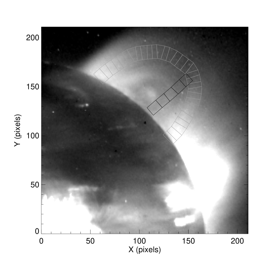
Figure 1:

Figure 2:

Figure 3:

Figure 4: