Fast CMB Power Spectrum Estimation of Temperature and Polarisation with Gabor Transforms

Abstract

We extend the analysis of Gabor transforms on a Cosmic Microwave Background (CMB) temperature map [Hansen, Górski & Hivon 2002] to polarisation. We study the temperature and polarisation power spectra on the cut sky, the so-called pseudo power spectra. The transformation kernels relating the full-sky polarisation power spectra and the polarisation pseudo power spectra are found to be similar to the kernel for the temperature power spectrum. This fact is used to construct a fast power spectrum estimation algorithm using the pseudo power spectrum of temperature and polarisation as data vectors in a maximum likelihood approach. Using the pseudo power spectra as input to the likelihood analysis solves the problem of having to invert huge matrices which makes the standard likelihood approach infeasible.

1 introduction

Most theories of the early universe predict the temperature and polarisation fluctuations of the CMB to be Gaussian distributed. In such models, the angular temperature and polarisation power spectra contain all the information about the cosmological parameters which one can determine from observations of the CMB sky. As several combinations of the cosmological parameters can give rise to similar temperature power spectra, estimating the polarisation power spectra will break the degeneracy and will be of great importance for accurate estimation of cosmological parameters. Also the error bars on these parameters can be reduced by exploiting the extra information present in the CMB polarisation power spectra.

Much effort has been made recently in order to find methods to analyse the CMB temperature power spectrum [Hansen, Górski & Hivon 2002, Oh, Spergel & Hinshaw 1999, Wandelt, Górski & Hivon 2000, Wandelt 2000, Wandelt & Hansen 2001, Bond 1995, Bond, Jaffe & Knox 2000, Bartlett et al. 2000, Tegmark 1997, Dore, Knox & Peel 2001, Szapudi et al. 2000, Hivon et al. 2002, Balbi et al. 2002]. There has been very few publications confronting the even harder task of estimating the polarisation power spectra. The framework for analysing the polarisation power spectra has been set in [Zaldarriaga & Seljak 1997, Kamionkowski, Kosowsky & Stebbins 1997] but these papers only describe the full likelihood method which is far too time consuming also when only considering the temperature power spectrum. In [Tegmark & de Oliveira-Costa 2001] a quadratic polarisation power spectrum estimation method was introduced, similar to the one presented in [Tegmark 1997] for temperature only.

In this paper we will extend the method of using the pseudo power spectrum as input to a likelihood estimation procedure of the power spectrum as described in [Hansen, Górski & Hivon 2002] (from now on called HGH). We will include the $E$ and $C$ mode polarisation pseudo power spectra in the data vector and use techniques similar to those described in HGH to estimate the power spectra. This can be done because the kernels that connect the full sky polarisation power spectra with the polarisation pseudo power spectra on an apodised sky are similar to the kernel for the temperature power spectrum. In the first part of this paper we will derive the formulae for these kernels and for the polarisation pseudo power spectra and discuss their shapes. Then in the second part this will be used for likelihood estimation.

In this paper the $B$ component polarisation will mostly be neglected. The $B$ polarisation power spectrum is expected to be very small and will hardly be detectable by the upcoming $MAP$ or $Planck$ satellite experiments [Jaffe, Kamionkowski & Wang 2001]. Also the $E$ and $B$ components of polarisation mix on the cut sky as will be discussed in this paper, making the $B$ polarisation pseudo spectrum to be dominated by the $E$ component [Lewis, Challinor & Turok 2001, Chiueh & Ma 2001, Tegmark & de Oliveira-Costa 2001, Bunn et al. 2002].

2 The Gabor Transformation

In this paper we will use the polarisation power spectra as they are defined in [Zaldarriaga & Seljak 1997]. There are three polarisation power spectra, $C^{E}_{\ell}$, $C^{B}_{\ell}$ and $C^{C}_{\ell}$. These are defined as

$$C^{E}_{\ell} = \sum_{m}\frac{a^{E}_{\ell m}a^{E*}_{\ell m}}{2\ell+1},$$ (1)

$$C^{B}_{\ell} = \sum_{m}\frac{a^{B}_{\ell m}a^{B*}_{\ell m}}{2\ell+1},$$ (2)

$$C^{C}_{\ell} = \sum_{m}\frac{a^{E}_{\ell m}a^{T*}_{\ell m}}{2\ell+1},$$ (3)

where the $a_{\ell m}$ coefficients are given in Appendix (E). In the following when we write the full sky power spectrum $C_{\ell}$ for temperature or polarisation, we will always mean the ensemble averaged power spectrum $\langle C_{\ell}\rangle$.

As discussed in more detail in HGH, the Gabor transformation of a dataset [Gabor 1946] is just the Fourier transformation of the dataset multiplied with a window function called the Gabor window. The window function can be used to cut out parts of the dataset in order to study only smaller segments of the dataset at a time. The window can be a top-hat window, just setting the unwanted parts of the dataset to zero. Another option is to use a function like a Gaussian to smooth the edges between the segment which one wants to study and the parts which are set to zero in order to avoid ringing in the Fourier spectrum. In HGH this formalism was extended to the sphere and used for CMB analysis. A disc on the CMB sky was cut out, using either a top-hat or a Gaussian window. The Gabor coefficients on this cut sky, called the pseudo power spectrum was expressed in terms of the full-sky power spectrum and the kernel connecting the full-sky and the cut-sky power spectrum was studied. The aim of this first section is to extend this to polarisation.

When multiplying the polarisation map with a Gabor window $G(\mathbf{n},\mathbf{n}_{0})$ which is axissymmetric about the point $\mathbf{n}_{0}$, the pseudo spectra on this apodised CMB sky can be written in terms of the full-sky spectra as (Appendix E)

$$\langle\tilde{C}_{\ell}^{E}\rangle = \sum_{\ell^{\prime}}C_{\ell^{\prime}}^{E}K_{2}(\ell,\ell^{\prime})+\sum_{\ell^{\prime}}C_{\ell^{\prime}}^{B}K_{-2}(\ell,\ell^{\prime}),$$ (5)

$$\langle\tilde{C}^{B}_{\ell}\rangle = \sum_{\ell^{\prime}}C_{\ell^{\prime}}^{B}K_{2}(\ell,\ell^{\prime})+\sum_{\ell^{\prime}}C_{\ell^{\prime}}^{E}K_{-2}(\ell,\ell^{\prime}),$$ (6)

$$\langle\tilde{C}^{C}_{\ell}\rangle = \sum_{\ell^{\prime}}C_{\ell^{\prime}}^{C}K_{20}(\ell,\ell^{\prime}),$$ (7)

where the kernels $K_{\pm 2}$ and $K_{20}$ are given in Appendix (E). These kernels are expression in terms of the $h_{2}(\ell,\ell^{\prime},m,m^{\prime})$ function which is defined similar to the $h(\ell,\ell^{\prime},m,m^{\prime})$ function used to express the kernel for the temperature power spectrum in HGH.

As with the temperature kernels, the polarisation kernels can be evaluated either using the analytical Wigner symbol expressions (134) and (137) or faster by direct integration and recursion of the $h_{2}(\ell,\ell^{\prime},m,m^{\prime})$ functions. The recursion for the $h_{2}(\ell,\ell^{\prime},m,m^{\prime})$ functions in Appendix (D) is one of the major results in this paper. This is an extension of the recursion for $h(\ell,\ell^{\prime},m,m^{\prime})$ derived in HGH.

In Appendix (E) and (F) we show that the polarisation pseudo power spectra are rotationally invariant. For this reason we will in the rest of the paper put the centre of the Gabor window on the north pole. This makes the calculations easier while keeping the generality of the results.

In this section we will study the Gabor kernel for a Gaussian and a top-hat Gabor window. The Gaussian is defined as

$$G(\theta)= e^{-\theta^{2}/(2\sigma^{2})} \theta\leq\theta_{C},$$ (9)

$$G(\theta)= 0 \theta>\theta_{C},$$ (10)

where we will use $5$ and $15$ degrees FWHM (corresponding to $\sigma=2.12^{\circ}$ and $\sigma=6.38^{\circ}$) and a cut-off angle $\theta_{C}=3\sigma$. We will also be comparing with a top-hat window covering the same area on the sky ($\theta_{C}$ is the same). The top-hat window is defined as

$$G(\theta)= 1 \theta\leq\theta_{C},$$ (11)

$$G(\theta)= 0 \theta>\theta_{C}.$$ (12)

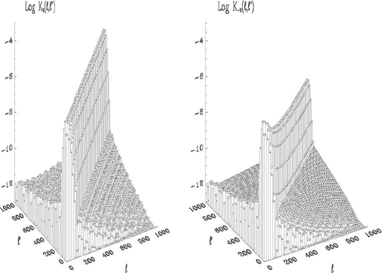
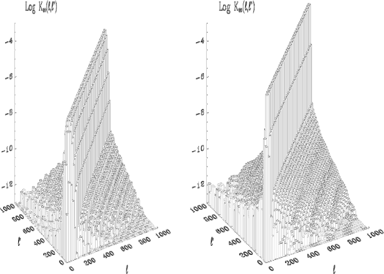
Studying equation (5) and (6) one sees that the $E$ and $B$ modes are mixing when only a portion of the sky is observed. The kernel $K_{2}(\ell,\ell^{\prime})$ is the kernel which takes full sky $C^{E}_{\ell}$ modes to the pseudo coefficients $\tilde{C}^{E}_{\ell}$ and similarly for $C^{B}_{\ell}$. The kernel $K_{-2}(\ell,\ell^{\prime})$ is the one which causes the mixing. In figure (1) and (2) we have plotted the kernels $K_{2}(\ell,\ell^{\prime})$ together with $K_{-2}(\ell,\ell^{\prime})$ for a $5$ and $15$ degree FWHM Gaussian Gabor window with $\theta_{C}=3\sigma$. One can see that the diagonal of the $K_{2}(\ell,\ell^{\prime})$ kernel is about an order of magnitude larger than the diagonal of the mixing kernel $K_{-2}(\ell,\ell^{\prime})$. This means that $C^{E}_{\ell}$ would dominate $\tilde{C}^{E}_{\ell}$ and $C^{B}_{\ell}$ would dominate $\tilde{C}^{B}_{\ell}$ provided that the two spectra $C^{E}_{\ell}$ and $C^{B}_{\ell}$ were of the same order of magnitude. However as discussed before, the $C^{B}_{\ell}$ are expected to be considerably smaller than $C^{E}_{\ell}$ in most cosmological models. For the $E$ mode this is not a problem as $C^{E}_{\ell}$ will then hardly be affected. The problem is the $B$ mode which in this case will be dominated by the $E$ mode.

Figure 1: The kernels $K_{2}(\ell,\ell^{\prime})$ (left plot) and $K_{-2}(\ell,\ell^{\prime})$ (right plot) connecting full and cut sky polarisation power spectra $C^{E}_{\ell}$ and $C^{B}_{\ell}$. The left kernel is the one which takes full sky $C^{E}_{\ell}$ into cut sky $\tilde{C}^{E}_{\ell}$ and full sky $C^{B}_{\ell}$ into cut sky $\tilde{C}^{B}_{\ell}$. The right kernel is the one which mixes the two giving contributions from full sky $C^{E}_{\ell}$ in cut sky $\tilde{C}^{B}_{\ell}$ and vice versa.

Figure 2: The same as figure (1) for a $15$ degree FWHM Gaussian Gabor window.

The separation of $E$ and $B$ modes of polarisation on the cut sky was already discussed in [Lewis, Challinor & Turok 2001, Chiueh & Ma 2001, Tegmark & de Oliveira-Costa 2001, Bunn et al. 2002]. We will in this paper assume that the $B$ mode polarisation component is neglible, but note that a possible extension of the power spectrum estimation method outlined here to $B$ mode polarisation would be to define

$$a_{+,\ell m} = a_{E,\ell m}+ia_{B,\ell m}$$ (13)

$$a_{-,\ell m} = a_{E,\ell m}-ia_{B,\ell m},$$ (14)

with the corresponding pseudo quantities

$$\tilde{a}_{+,\ell m} = \sum_{\ell^{\prime}}a_{+,\ell^{\prime}m}(H_{2}(\ell,\ell^{\prime},m)+H_{-2}(\ell,\ell^{\prime},m)),$$ (15)

$$\tilde{a}_{-,\ell m} = \sum_{\ell^{\prime}}a_{-,\ell^{\prime}m}(H_{2}(\ell,\ell^{\prime},m)-H_{-2}(\ell,\ell^{\prime},m)),$$ (16)

written in terms of the $H_{2}$ functions defined in Appendix (E). For the power spectra one gets,

$$\langle C^{+}_{\ell}\rangle \equiv \sum_{m}\frac{\langle a_{+,\ell m}a_{+,\ell m}^{*}\rangle}{2\ell+1}=\langle C^{E}_{\ell m}\rangle+\langle C^{B}_{\ell m}\rangle,$$ (18)

$$\langle C^{-}_{\ell}\rangle \equiv \sum_{m}\frac{\langle a_{-,\ell m}a_{-,\ell m}^{*}\rangle}{2\ell+1}=\langle C^{E}_{\ell m}\rangle-\langle C^{B}_{\ell m}\rangle.$$ (19)

To get the pseudo power spectra one can use equations (15) and (16) to get

$$\langle\tilde{C}^{+}_{\ell}\rangle = \sum_{\ell^{\prime}}C^{+}_{\ell}K_{+}(\ell,\ell^{\prime}),$$ (21)

$$\langle\tilde{C}^{-}_{\ell}\rangle = \sum_{\ell^{\prime}}C^{-}_{\ell}K_{-}(\ell,\ell^{\prime}),$$ (22)

where the kernels can be written

$$K_{+}(\ell,\ell^{\prime}) = \frac{1}{2\ell+1}\sum_{m}(H_{2}(\ell,\ell,m)+H_{-2}(\ell,\ell^{\prime},m))^{2},$$ (23)

$$K_{-}(\ell,\ell^{\prime}) = \frac{1}{2\ell+1}\sum_{m}(H_{2}(\ell,\ell,m)-H_{-2}(\ell,\ell^{\prime},m))^{2}.$$ (24)

Separation of $E/B$ modes will not be discussed further in this paper as this is extensively treated in the references above.

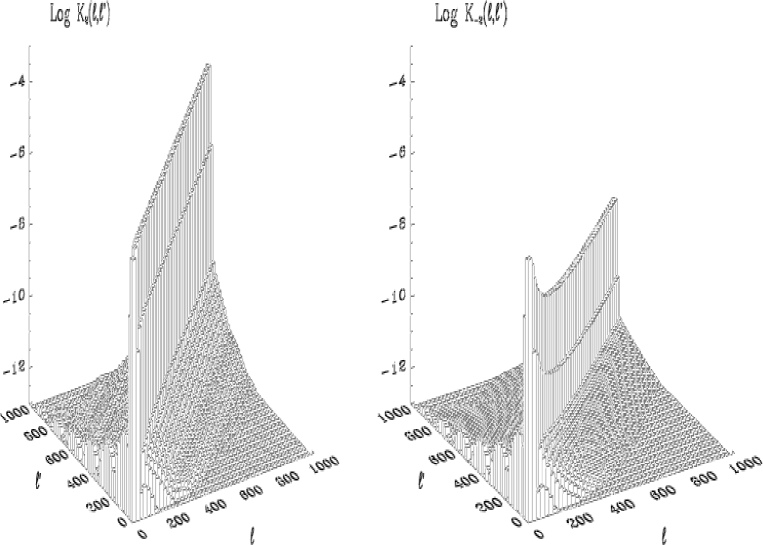
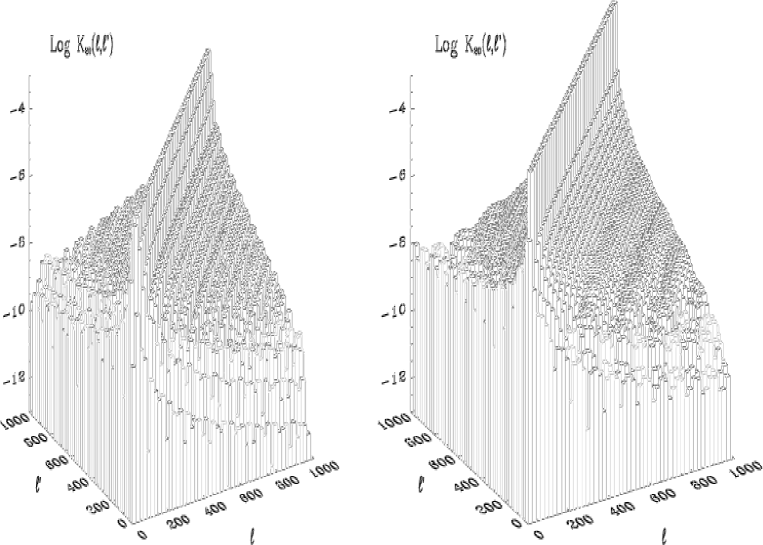
In figure (3) and (4) we have plotted the $K_{2}(\ell,\ell^{\prime})$ and $K_{-2}(\ell,\ell^{\prime})$ kernels for a tophat window covering the same area on the sky as the Gaussian windows in figure (1) and (2).

Figure 3: The same as figure (1) for a tophat Gabor window covering the same area on the sky as the Gaussian window in figure (1)

Figure 4: The same as figure (2) for a tophat Gabor window covering the same area on the sky as the Gaussian window in figure (2)

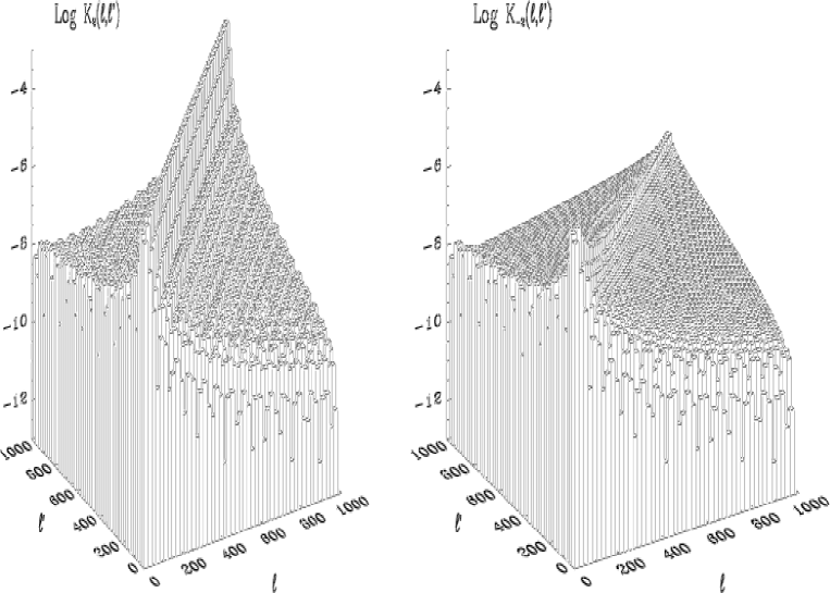
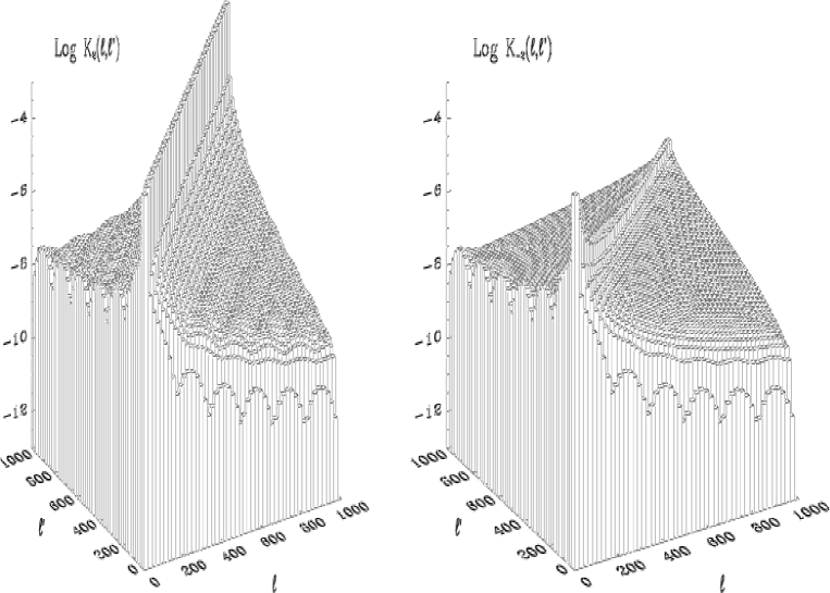
The kernel $K_{20}(\ell,\ell^{\prime})$ for the cross polarisation power spectrum $C^{C}_{\ell}$ is shown in figure (5) for a $5$ and $15$ degree Gaussian window and in figure (6) for the corresponding tophat windows.

Figure 5: The kernel $K_{20}(\ell,\ell^{\prime})$ connecting the full sky cross polarisation spectrum $C^{C}_{\ell}$ and the cut sky spectrum $\tilde{C}^{C}_{\ell}$ for a $5$ (left plot) and $15$ (right plot) degree FWHM Gaussian Gabor window. The negative elements have a brighter colour.

Figure 6: Same as figure (5) for the corresponding tophat windows.

As for the temperature kernels, all the polarisation kernels show the same behaviour when changing type and size of the window. When going from smaller to larger windows, the diagonals get sharper. Also the tophat kernels have more long range correlations than the Gaussian kernels (note that all the plots have the same vertical scale and can be compared directly).

In figure (7) we have plotted slices of the different kernels at $\ell=200$ for comparison. The slices are made of the kernels for $5$ and $15$ degree FWHM Gaussian Gabor windows. The first thing to note is that the temperature kernel $K(\ell,\ell^{\prime})$, the $E$ and $B$ kernel $K_{2}(\ell,\ell^{\prime})$ and the temperature-polarisation cross spectrum kernel $K_{20}(\ell,\ell^{\prime})$ only differ for the far off-diagonal elements. At the diagonal their shape and size are the same. For this reason the relation shown in HGH between the width of the kernel and the width of the size of the window for the temperature power spectrum is also valid for polarisation. This is an important result to be used for the likelihood estimation of the polarisation power spectra in the next section. It shows that the number of polarisation pseudo spectrum coefficients to be used in the likelihood analysis should be the same as for the likelihood estimation of the temperature power spectrum.

In figure (8) a similar plot is shown for the corresponding tophat windows. The plot shows that the conclusions made for the Gaussian windows are also valid in this case. The shape and size of the three kernels are the same around the diagonal. For this reason the results shown for the temperature kernel that the tophat window has larger long range correlations whereas the Gaussian window has large short range correlations and therefore a wider kernel is also valid for polarisation.

Figure 7: A slice at $\ell=200$ of the kernels combining the full sky and cut sky power spectra. The thick solid line is the kernel $K(\ell,\ell^{\prime})$ for the temperature power spectrum, the thin solid line is the kernel $K_{2}(\ell,\ell^{\prime})$ for $E$ and $B$ mode polarisation and the dotted line is the kernel for the temperature-polarisation cross power spectrum $K_{20}(\ell,\ell^{\prime})$. All these kernels go together around the diagonal. They only differ for the far off-diagonal elements. The dashed line is the mixing kernel $K_{-2}(\ell,\ell^{\prime})$ which mixes the $E$ and $B$ mode polarisation power spectra on the cut sky. This kernel is lower than the other kernels. The upper plot is for a $5$ degree Gaussian Gabor window and the lower plot for a $15$ degree FWHM Gaussian window.

Figure 8: Same as figure (7) but for tophat windows covering the same area on the sky.

The kernel $K_{-2}(\ell,\ell^{\prime})$ which mixes the $E$ and $B$ modes on the cut sky is plotted as a dashed line in figures (7) and (8). It is much smaller than the three other kernels and the shape seems to differ as well. Note that the height of the mixing kernel relative to the other kernels is lower for the $15$ degree window than for the $5$ degree window. That the size of the mixing kernel relative to the other kernels is dropping when the size of the window is increasing was to be expected since in the limit of full sky coverage the $E$-$B$ mixing disappears and the mixing kernel must go to zero.

In figure (9) a slice at $\ell=200$ of the temperature kernel and the mixing kernel is shown for the $5$ and $15$ degree FWHM Gaussian Gabor window. The kernels are normalised to one at the peak so that the shapes can be compared. For the Gaussian window, the shapes of the kernels still seem to be the same. But the kernels for the corresponding tophat windows shown in figure (10) does not have a Gaussian shape and differs significantly from the other kernels.

Figure 9: A slice at $\ell=200$ of the kernel $K(\ell,\ell^{\prime})$ connecting the full sky temperature power spectrum with the cut sky temperature power spectrum (solid line) and the kernel $K_{-2}(\ell,\ell^{\prime})$ which is mixing the $E$ and $B$ mode polarisation power spectra on the cut sky. The upper plot is for a $5$ degree FWHM Gaussian Gabor window and the lower plot for a $15$ degree Gaussian window. The kernels are here normalised to $1$ at the peak at $\ell=200$ in order to compare the shapes of the kernels.

Figure 10: This figure is the same as figure (9) for tophat windows covering the same area on the sky.

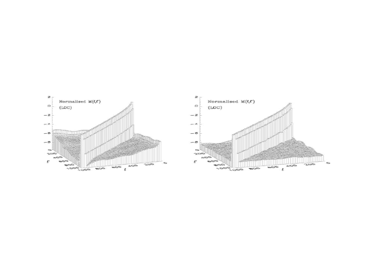
Since the kernels for the polarisation power spectra have a shape similar to that of the temperature power spectrum the effect of a Gabor window on the shape of the power spectrum should also be similar. This can be seen in figure (11) and (12). The figures show the full sky polarisation power spectra (dashed line) $C_{\ell}^{E}$ (figure 11) and $C_{\ell}^{C}$ (figure 12) for a standard CDM model. In this model the $B$ component of polarisation is zero. On top of the full sky power spectra we have plotted the polarisation pseudo power spectra for a $5$ and $15$ degree Gaussian Gabor window (upper and lower plots respectively) normalised so that it can be compared to the full sky spectrum. The pseudo spectra for the corresponding tophat windows are plotted as dotted lines. As expected the shape of the polarisation pseudo spectra relative to the full sky spectra is similar to that for the temperature spectrum shown in HGH. One difference is that the polarisation pseudo spectra for the Gaussian window do not have the characteristic extra peak at low multipole which is seen in the temperature pseudo spectrum. This peak in the temperature spectrum arose due to the steep $1/\ell(\ell+1)$ fall-off of the temperature spectrum at low multipole. The polarisation spectra do not have this steep fall-off and for this reason there is no extra peak.

Figure 11: The windowed polarisation power spectra $\tilde{C}_{\ell}^{E}$ for a $5$ and $15$ degree FWHM Gaussian Gabor window cut at $\theta_{C}=3\sigma$ (solid line) and for a tophat window covering the same area on the sky (dotted line). All spectra are normalised in such a way that they can be compared directly with the full sky spectrum which is shown on each plot as a dashed line. Only in the first plot are all three lines visible. In the three last plots, the full sky spectrum and the Gaussian pseudo spectrum (dashed and solid line) are hardly distinguishable.

Figure 12: Same as figure (11) for the temperature-polarisation cross power spectrum $C^{C}_{\ell}$.

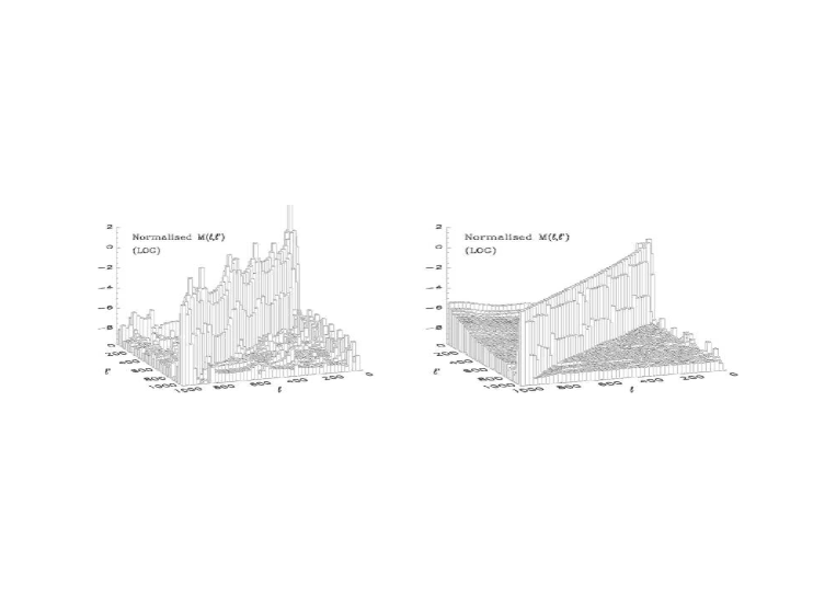
Because of the mixing of $E$ and $B$ modes there is also a $B$ polarisation component $\tilde{C}^{B}_{\ell}$ for the pseudo spectrum even when the input full sky $C^{B}_{\ell}$ were zero. This is shown in figure (13) where we have plotted the full sky spectrum $C^{E}_{\ell}$ and the pseudo spectra $\tilde{C}_{\ell}^{B}$ for the $5$ and $15$ degree FWHM Gaussian Gabor windows and corresponding tophat windows. The pseudo spectra are normalised so that they can be compared directly to the full sky spectrum. The dashed lines show the pseudo spectra for the Gaussian window. The upper line is for the $5$ degree window and the lower line for the $15$ degree window. As expected the size of the $B$ component is dropping with increasing window size. The $\tilde{C}^{B}_{\ell}$ for the tophat windows are plotted as dotted lines. The shape of the pseudo spectra $\tilde{C}^{B}_{\ell}$ for the Gaussian windows are roughly following the shape of the full sky $C^{E}_{\ell}$. This could be expected because the mixing kernel $K_{-2}(\ell,\ell^{\prime})$ for the Gaussian window has a Gaussian shape close to the diagonal, similar to the other kernels (see figure (9)). The pseudo spectra $C^{B}_{\ell}$ for the tophat windows however are much smoother due to the much broader kernel (figure 10).

Figure 13: The full sky $C^{E}_{\ell}$ power spectrum plotted together with the spectra $\tilde{C}^{B}_{\ell}$ on the windowed sky. The dashed lines show the $B$ spectra for a $5$ and $15$ degree FWHM Gaussian Gabor window (upper and lower line respectively). The dotted lines are for the corresponding tophat windows. The pseudo spectra are normalised so that they can be compared directly with the full sky spectrum. In the model used, there was no $B$ polarisation spectrum for the full sky. The $\tilde{C}^{B}_{\ell}$ shown arise due to the mixing of $E$ and $B$ modes on the cut sky only.

In the same way as for the temperature power spectrum, we have shown that the polarisation pseudo spectra resemble the full sky polarisation spectra when the patches on the sky are large enough. This motivates the use of the polarisation pseudo power spectra as input to a likelihood estimation of the polarisation power spectra in the same way as for the temperature power spectrum showed in HGH. To do likelihood analysis one needs to find theoretical expressions for the correlations between different $\tilde{C}_{\ell}^{Z}$ (Z={T,E,C}).

3 Likelihood Analysis

In HGH a Gaussian likelihood ansatz with the pseudo power spectrum as the input data was successfully used to estimate the power spectrum. Because of the similarities between the kernels of the polarisation power spectra and the temperature power spectrum we can assume that this works for the estimation of the polarisation power spectra as well. We will now show the results of some Monte Carlo simulations confirming this assumption. In this section we will assume that the $B$ component of polarisation is so small that it can be neglected. We will only concentrate on the $T$, $E$ and $C$ components as in most standard theories of the early universe the $B$ component will be too small to be measured by the MAP and Planck satellite experiments [Jaffe, Kamionkowski & Wang 2001].

In figure (14) and (15) we have plotted the probability distribution of the $\tilde{C}^{E}_{\ell}$ and $\tilde{C}^{C}_{\ell}$ from 10000 simulations. The probability distribution (histogram) is plotted on top of a Gaussian (dashed line) with mean and FWHM taken from the theoretical expressions derived in Appendix (G). In these simulations we were using a $5$ degree FWHM Gaussian Gabor window with $\theta_{C}=3\sigma$. In figure (16) and (17) we show the results of similar simulations with a $15$ degree FWHM Gaussian Gabor window. As expected the trend is that the distributions get more and more Gaussian for higher multipoles and for bigger windows. For the $15^{\circ}$ FWHM window, the distribution is very close to a Gaussian for the multipoles above $\ell=50$.

Figure 14: The probability distribution of $\tilde{C}^{E}_{\ell}$ taken from 10000 simulations with a $5^{\circ}$ FWHM Gaussian Gabor window truncated at $\theta_{C}=3\sigma$. The variable $x$ is given as $x=(\tilde{C}^{E}_{\ell}-\langle\tilde{C}^{E}_{\ell}\rangle)/\sqrt{\langle(\tilde{C}^{E}_{\ell}-\langle\tilde{C}^{E}_{\ell}\rangle)^{2}\rangle}$. The dashed line is a Gaussian with the theoretical mean and standard deviation of the $\tilde{C}^{E}_{\ell}$. The plot shows the $\tilde{C}^{E}_{\ell}$ distribution for $\ell=50$, $\ell=200$, $\ell=500$, and $\ell=800$. The probabilities are normalised such that the integral over $x$ is $1$.

Figure 15: Same as figure (14) for the temperature-polarisation cross spectra $\tilde{C}^{C}_{\ell}$.

Figure 16: Same as figure (14) for a $15^{\circ}$ FWHM Gaussian Gabor window.

Figure 17: Same as figure (15) for a $15^{\circ}$ FWHM Gaussian Gabor window.

Figure (18) and (19) show the probability distribution for a tophat window covering the same area on the sky as the Gaussian window used in figure (16) and (17). Also this distribution is very close to a Gaussian.

Figure 18: Same as figure (16) for a tophat window covering the same area on the sky

Figure 19: Same as figure (17) for a tophat window covering the same area on the sky

The previous plots have shown that a Gaussian likelihood ansatz for the polarisation pseudo spectra seems to be a very good approximation provided that the window is big enough. As for the temperature spectrum, the approximation is no longer valid for the lowest multipoles, but as was shown for the temperature power spectrum, this might only give rise to a very small downward bias for the estimates of the lowest multipoles.

The form of the log-likelihood to minimise is therefore still

$$L=\mathbf{d}^{T}\mbox{$\textbf{{M}}$}^{-1}\mathbf{d}+\ln{\det{\mbox{$\textbf{{M}}$}}},$$ (25)

where the data vector now consists of the temperature and polarisation power spectra $\mathbf{d}=\{\mathbf{d}^{T},\mathbf{d}^{E},\mathbf{d}^{C}\}$. Here the $\mathbf{d}^{Z}$ vectors are given as

$$d_{i}^{Z}=\tilde{C}_{\ell_{i}}^{Z}-\langle\tilde{C}_{\ell_{i}}^{Z}\rangle,$$ (26)

where $Z=\{T,E,B\}$. Similarly the correlation matrix M will consist of blocks $\mbox{$\textbf{{M}}$}_{ZZ^{\prime}}$ defined as

$$M_{ZZ^{\prime},ij}=\langle\tilde{C}_{\ell_{i}}^{Z}\tilde{C}_{\ell_{j}}^{Z^{\prime}}\rangle-\langle\tilde{C}_{\ell_{i}}^{Z}\rangle\langle\tilde{C}_{\ell_{j}}^{Z^{\prime}}\rangle.$$ (27)

This structure of the data vector and correlation matrix is shown in figure (20).

Figure 20: The figure shows the structure of the datavector $\mathbf{d}$ on the left hand side and the correlation matrix M on the right hand side used for joint likelihood estimation of temperature and polarisation power spectra.

For fast likelihood estimation, it is crucial that one can calculate the average pseudo spectra $\langle\tilde{C}^{Z}_{\ell}\rangle$ and correlation matrix M fast. The formalism in HGH which enabled fast calculations of these quantities for the temperature power spectrum is extended to polarisation in Appendix (G) (signal) and Appendix (H) (noise).

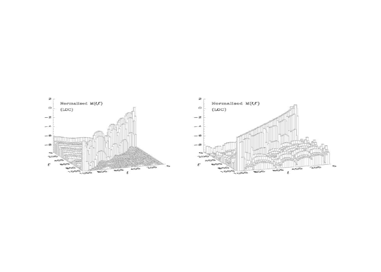
In figure (21) we have plotted the signal correlation matrix $M^{TT}_{\ell\ell^{\prime}}$ next to the matrix $M^{EE}_{\ell\ell^{\prime}}$. A standard CDM power spectrum without $B$ mode polarisation was used. The two matrices are very similar. One big difference is that the matrix for $E$ mode polarisation is missing the ’wall’ at low multipoles present in the temperature matrix. As discussed before this is because of the different shapes for the $T$ and $E$ power spectra at low multipoles. The temperature power spectrum drops steeply at low $\ell$ while this is not the case for the $E$ mode polarisation spectrum.

Figure 21: The correlation matrices $M(\ell,\ell^{\prime})$ in the figure show the correlations between the temperature pseudo power spectrum coefficients and between the $E$ mode polarisation pseudo spectrum coefficients for a $15$ degree FWHM Gaussian Gabor window. The left plot shows $(\langle\tilde{C}^{T}_{\ell}\tilde{C}^{T}_{\ell^{\prime}}\rangle-\langle\tilde{C}^{T}_{\ell}\rangle\langle\tilde{C}^{T}_{\ell^{\prime}}\rangle)/(\langle\tilde{C}^{T}_{\ell}\rangle\langle\tilde{C}^{T}_{\ell^{\prime}}\rangle)$ and the right plot shows $(\langle\tilde{C}^{E}_{\ell}\tilde{C}^{E}_{\ell^{\prime}}\rangle-\langle\tilde{C}^{E}_{\ell}\rangle\langle\tilde{C}^{E}_{\ell^{\prime}}\rangle)/(\langle\tilde{C}^{E}_{\ell}\rangle\langle\tilde{C}^{E}_{\ell^{\prime}}\rangle)$. A standard CDM power spectrum was used to produce the plots.

In figures (22) and (23) the $M^{CC}_{\ell\ell^{\prime}}$, $M^{TC}_{\ell\ell^{\prime}}$, $M^{TE}_{\ell\ell^{\prime}}$ and $M^{EC}_{\ell\ell^{\prime}}$ matrices are shown. All matrices are diagonally dominant and since the values on the diagonals all have the same order of magnitude, they all have to be included in the total matrix $M$.

Figure 22: The correlation matrices $M(\ell,\ell^{\prime})$ in the figure show the correlations between the cross-correlation pseudo power spectrum $C$ coefficients and between the temperature and cross correlation pseudo spectrum coefficients $C$ for a $15$ degree FWHM Gaussian Gabor window. The left plot shows $(\langle\tilde{C}^{C}_{\ell}\tilde{C}^{C}_{\ell^{\prime}}\rangle-\langle\tilde{C}^{C}_{\ell}\rangle\langle\tilde{C}^{C}_{\ell^{\prime}}\rangle)/(\langle\tilde{C}^{C}_{\ell}\rangle\langle\tilde{C}^{C}_{\ell^{\prime}}\rangle)$ and the right plot shows $(\langle\tilde{C}^{T}_{\ell}\tilde{C}^{C}_{\ell^{\prime}}\rangle-\langle\tilde{C}^{T}_{\ell}\rangle\langle\tilde{C}^{C}_{\ell^{\prime}}\rangle)/(\langle\tilde{C}^{T}_{\ell}\rangle\langle\tilde{C}^{C}_{\ell^{\prime}}\rangle)$. A standard CDM power spectrum was used to produce the plots.

Figure 23: The correlation matrices $M(\ell,\ell^{\prime})$ in the figure show the correlations between the temperature and $E$ mode polarisation pseudo spectrum coefficients and between the $E$ mode polarisation and cross correlation pseudo spectrum coefficients $C$ for a $15$ degree FWHM Gaussian Gabor window. The left plot shows $(\langle\tilde{C}^{T}_{\ell}\tilde{C}^{E}_{\ell^{\prime}}\rangle-\langle\tilde{C}^{T}_{\ell}\rangle\langle\tilde{C}^{E}_{\ell^{\prime}}\rangle)/(\langle\tilde{C}^{T}_{\ell}\rangle\langle\tilde{C}^{E}_{\ell^{\prime}}\rangle)$ and the right plot shows $(\langle\tilde{C}^{E}_{\ell}\tilde{C}^{C}_{\ell^{\prime}}\rangle-\langle\tilde{C}^{E}_{\ell}\rangle\langle\tilde{C}^{C}_{\ell^{\prime}}\rangle)/(\langle\tilde{C}^{E}_{\ell}\rangle\langle\tilde{C}^{C}_{\ell^{\prime}}\rangle)$. A standard CDM power spectrum was used to produce the plots.

4 Results of Likelihood Estimations

The likelihood estimation was carried out in the same way as for the temperature power spectrum. As discussed in HGH, when we observe the cut-sky we do not have enough information to estimate the full-sky $C_{\ell}$ for all multipoles. One has to estimate the $C_{\ell}$ in $N^{bin}$ bins. Also, the $\tilde{C}_{\ell}$ coefficients are not independent on the cut sky, so a limited number $N^{in}\leq N^{bin}$ of pseudo spectrum coefficients have to be used as input to the likelihood. How many multipoles depends on the width $\Delta\ell$ of the Gabor kernel for a given window which is discussed in more detail in HGH.

The power spectra were estimated in bins defined as

$$C^{T}_{\ell} = \frac{D^{T}_{b}}{\ell(\ell+1)},\ \ \ell_{b}\leq\ell<\ell_{b+1},$$ (28)

$$C^{E}_{\ell} = \frac{D^{E}_{b}}{\ell(\ell+1)},\ \ \ell_{b}\leq\ell<\ell_{b+1},$$ (29)

where $\ell_{b}$ is the first multipole in bin $b$. A similar binning does not work for for the temperature-polarisation cross correlation power spectrum. The reason for this is the Schwarz inequality $C^{C}_{\ell}\leq\sqrt{C^{T}_{\ell}C^{E}_{\ell}}$. During likelihood maximisation one must make sure that the estimated value of $C^{C}_{\ell}$ never exceeds $\sqrt{C^{T}_{\ell}C^{E}_{\ell}}$. The way we solved this problem was to estimate for $C^{C}_{\ell}/\sqrt{C^{T}_{\ell}C^{E}_{\ell}}$ under the constraint that this value never exceeds $1$. So the binning is then

$$C^{C}_{\ell} = D^{C}_{b}\sqrt{C^{T}_{\ell}C^{E}_{\ell}}$$ (31)

$$= \frac{D^{C}_{b}\sqrt{D^{T}_{b}D^{E}_{b}}}{\ell(\ell+1)},$$ (32)

where as before $\ell_{b}\leq\ell<\ell_{b+1}$.

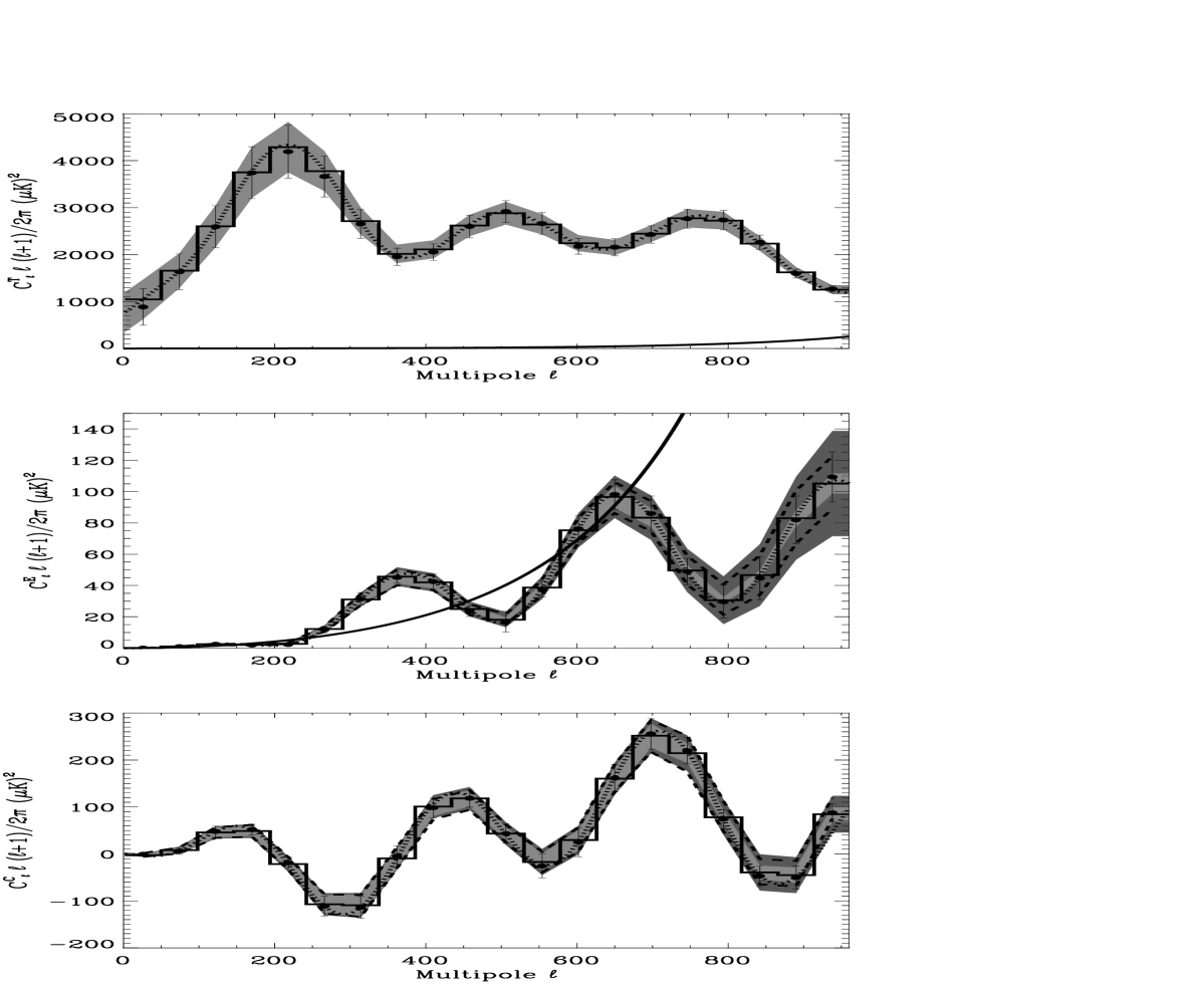
As an example we simulated a sky using $N_{side}=512$ resolution in Healpix [Górski, Hivon and Wandelt 1998] and a $10^{\prime}$ beam. We added non-uniform noise to the map. A reasonable assumption about the size of the noise deviations for polarisation is to take $\sigma^{P}_{j}=\sqrt{2}\sigma^{T}_{j}$ [Zaldarriaga & Seljak 1997]. This is what we used in this test, but note that the formalism do not require any relation between $\sigma_{T}$ and $\sigma_{P}$. The noise level was set so that the signal to noise ration for the temperature power spectrum was always well above $1$ below the maximum multipole $\ell=1024$ whereas for the $E$ mode polarisation power spectrum it was mostly below $1$ (see figure (25)). This is close to the values expected for the Planck HFI $143GHz$ [Bersanelli et al. 1996] channel. For the analysis we used a $15$ degree Gaussian Gabor window. The result of one single estimation is shown in figure (25). In this estimation we used $N^{in}=100$ pseudo spectrum multipoles as input and estimated for $N^{bin}=20$ multipole bins for each of the $T$, $E$ and $C$ modes.

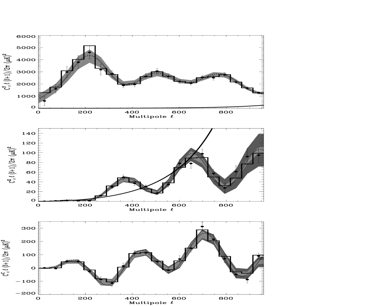
To test whether the method is bias or not, we did 60 Monte Carlo simulations. The result of the average of these simulations is shown in figure (24). The method seems to be unbiased also for the estimates of the polarisation power spectra. Note that the expected noise variance taken from the often used analytic formula for uniform noise (shaded areas on the plot) given in [Hivon et al. 2002] and HGH here fails to predict the size of the error bars on the estimates. The expected variance taken from the inverse Fisher matrix (dashed lines) fits better with the error bars from Monte Carlo. The reason is that we used a noise profile with increasing noise from the centre of the disc and down to the edges, opposite of the Gaussian window. This gives the observation with high $S/N$ higher significance in the analysis. This is similar to a result for the temperature power spectrum discussed further in HGH.

5 Discussion

We have presented a maximum likelihood method to simultaneously estimate the temperature and polarisation power spectra from high resolution CMB data in the presence of non-uniform noise and a symmetric Gabor window. An extension of the power spectrum estimation method developed in HGH has been made in order to estimate for the polarisation power spectra in addition to the temperature power spectrum. In most standard theories for the early universe, the $B$ component polarisation will be too small to be observed by the MAP and Planck experiments. For this reason, the method has been tested here under the assumption that the $B$ mode polarisation is negligible. In this case the method appears to give unbiased estimates of the polarisation power spectra also in the presence of non-uniform noise and a Gabor window.

The kernels connecting the full sky polarisation power spectra with the cut sky polarisation pseudo power spectra were studied and found to be very similar to the kernel for the temperature power spectrum. For this reason the effect of a cut sky and a Gabor window on the polarisation power spectra is similar to the effect on the temperature power spectrum. This explains that the method of estimating the power spectrum from the pseudo power spectrum for polarisation was as successful as it was for temperature.

One issue which has not been studied fully here is the inclusion of the $B$ mode polarisation. We demonstrated that the $E$ and $B$ mode polarisation power spectra are mixing on the cut sky making detections of the much weaker $B$ component difficult. Further work needs to be done in order to include the $B$ component in the likelihood analysis.

In HGH it was discussed how one can find the noise correlation matrix for temperature using Monte Carlo. This might be faster than the analytical approach presented here when the size of the dataset is very huge. With a sufficient number of Monte Carlo simulations this was shown to give similar error bars as the analytic treatment. The results for the temperature noise matrix is expected to be valid also for the polarisation noise matrices and can be used when the dataset is so big that the Monte-Carlo approach is significantly faster, or when correlated noise is present.

Another extension which was discussed in HGH was the simultaneous analysis of several patches on the CMB sky. This extension was shown to work for the temperature power spectrum and we expect that this could work also for polarisation, allowing data from several different experiments to be analysed together. In HGH it was shown that with this power spectrum estimation method, huge datasets like the ones to be expected from MAP or Planck can be analysed in a reasonable amount of time. The most time-consuming step in the method is the construction of the correlation matrix, which in the case of polarisation is 9 times longer. This makes also the joint temperature and polarisation power spectrum estimation feasible for huge datasets.

Figure 24: The result of a joint likelihood estimation of the temperature power spectrum (upper plot) and the $E$ (middle plot) and $C$ (lower plot) polarisation power spectra. The dotted line shows the full sky average spectrum. The histogram shows the binned input pseudo spectrum without noise. The shaded areas around the binned average full sky power spectrum (not shown) show the expected deviations from the average using the approximate formula for uniform noise. The bright shaded area shows the cosmic and sample variance only whereas the dark shaded area also shows expected variance due to noise. The dots show the estimate with $1\sigma$ error bars taken from the inverse Fisher matrix. In the analysis a $15$ degree FWHM Gaussian Gabor window with a $\theta_{C}=3\sigma$ cutoff was used.

Figure 25: Same as figure (24) but the dots here are the average of 60 estimates from Monte Carlo simulations. The error bars are the average deviations taken from the simulations. The dotted line shows the average full sky spectrum. The shaded areas which are plotted around the binned full sky power spectrum (not shown) show the variance taken from the approximate variance formula for uniform noise. The dashed lines show the expected variance taken from the inverse Fisher matrix.

Appendix A Rotation Matrices

A spherical function $T(\mathbf{\hat{n}})$ is rotated by the operator $\hat{D}(\alpha\beta\gamma)$ where $\alpha\beta\gamma$ are the three Euler angles for rotations [Risbo 1996] and the inverse rotation is $\hat{D}(-\gamma-\beta-\alpha)$. For the spherical harmonic functions, this operator takes the form,

$$Y_{\ell m}(\mathbf{\hat{n}}^{\prime})=\sum_{m^{\prime}=-\ell}^{\ell}D_{m^{\prime}m}^{\ell}(\alpha\beta\gamma)Y_{\ell m^{\prime}}(\mathbf{\hat{n}}),$$ (33)

where $D_{m^{\prime}m}^{\ell}$ has the form

$$D_{m^{\prime}m}^{\ell}(\alpha\beta\gamma)=e^{im^{\prime}\alpha}d_{m^{\prime}m}^{\ell}(\beta)e^{im\gamma}.$$ (34)

Here $d_{m^{\prime}m}^{\ell}(\beta)$ is a real coefficient with the following property:

$$d_{m^{\prime}m}^{\ell}(\beta)=d_{mm^{\prime}}^{\ell}(-\beta).$$ (35)

The D-functions also have the following property:

$$D_{m^{\prime}m}^{\ell}(\alpha\beta\gamma)=\sum_{m^{\prime\prime}}D_{m^{\prime}m^{\prime\prime}}^{\ell}(\alpha_{2}\beta_{2}\gamma_{2})D_{m^{\prime\prime}m}^{\ell}(\alpha_{1}\beta_{1}\gamma_{1}),$$ (36)

where $(\alpha\beta\gamma)$ is the result of the two consecutive rotations $(\alpha_{1}\beta_{1}\gamma_{1})$ and $(\alpha_{2}\beta_{2}\gamma_{2})$.

The complex conjugate of the rotation matrices can be written as

$$D^{\ell*}_{mm^{\prime}}=(-1)^{m+m^{\prime}}D^{\ell}_{(-m)(-m^{\prime})}.$$ (37)

See also Appendix (B).

Appendix B Spin-s Harmonics

The spherical harmonic functions $Y_{\ell m}(\mathbf{\hat{n}})$ can be generalised to spin-s harmonics using the rotation matrices in Appendix (A). The general definition is

$$D^{\ell}_{-sm}(\phi_{2},\theta,\phi_{1})=\sqrt{\frac{4\pi}{2\ell+1}}\ _{s}Y_{\ell m}(\theta,\phi_{2})e^{-is\phi_{1}},$$ (38)

or in the form which will be mostly used in this paper

$${}_{s}Y_{\ell m}(\theta,\phi)=\sqrt{\frac{2\ell+1}{4\pi}}D^{\ell}_{-sm}(\phi,\theta,0).$$ (39)

The spin-s harmonics have the orthogonality and completeness relations given by

$$\int d\mathbf{\hat{n}}\ _{s}Y_{\ell m}(\mathbf{\hat{n}})\ _{s}Y_{\ell m}(\mathbf{\hat{n}}) = \delta_{\ell\ell^{\prime}}\delta_{mm^{\prime}}$$ (40)

$$\sum_{\ell m}\ {}_{s}Y_{\ell m}(\mathbf{\hat{n}})\ _{s}Y_{\ell m}(\mathbf{\hat{n}}_{0}) = \delta(\mathbf{\hat{n}}-\mathbf{\hat{n}}_{0}).$$ (41)

The complex conjugate of the spin harmonics can be written

$$_{s}Y_{\ell m}^{*}(\mathbf{\hat{n}})=(-1)^{s+m}\ _{-s}Y_{\ell(-m)}(\mathbf{\hat{n}}).$$ (42)

Appendix C Some Wigner Symbol Relations

Throughout the paper, the Wigner 3j Symbols will be used frequently. Here are some relations for these symbols, which are used. The orthogonality relation is,

$$\sum_{mm^{\prime}}{\left(\begin{array}[]{ccc}\ell&\ell^{\prime}&\ell^{\prime\prime}\\ m&m^{\prime}&m^{\prime\prime}\\ \end{array}\right)}{\left(\begin{array}[]{ccc}\ell&\ell^{\prime}&L^{\prime\prime}\\ m&m^{\prime}&M^{\prime\prime}\\ \end{array}\right)}=(2\ell^{\prime\prime}+1)^{-1}\delta_{\ell^{\prime\prime}L^{\prime\prime}}\delta_{m^{\prime\prime}M^{\prime\prime}}.$$ (43)

The Wigner 3j Symbols can be represented as an integral of rotation matrices (see Appendix(A)),

$$\frac{1}{8\pi^{2}}\int d\cos\theta d\phi d\gamma D_{m_{1}m^{\prime}_{1}}^{\ell}D_{m_{2}m^{\prime}_{2}}^{\ell^{\prime}}D_{m_{3}m^{\prime}_{3}}^{\ell^{\prime\prime}}={\left(\begin{array}[]{ccc}\ell&\ell^{\prime}&\ell^{\prime\prime}\\ m_{1}&m_{2}&m_{3}\\ \end{array}\right)}{\left(\begin{array}[]{ccc}\ell&\ell^{\prime}&\ell^{\prime\prime}\\ m^{\prime}_{1}&m^{\prime}_{2}&m^{\prime}_{3}\\ \end{array}\right)}.$$ (44)

This expression can be reduced to,

$$\int d\mathbf{\hat{n}}Y_{\ell m}(\mathbf{\hat{n}})Y_{\ell^{\prime}m^{\prime}}(\mathbf{\hat{n}})Y_{\ell^{\prime\prime}m^{\prime\prime}}(\mathbf{\hat{n}})=\sqrt{\frac{(2\ell+1)(2\ell^{\prime}+1)(2\ell^{\prime\prime}+1)}{4\pi}}{\left(\begin{array}[]{ccc}\ell&\ell^{\prime}&\ell^{\prime\prime}\\ m&m^{\prime}&m^{\prime\prime}\\ \end{array}\right)}{\left(\begin{array}[]{ccc}\ell&\ell^{\prime}&\ell^{\prime\prime}\\ 0&0&0\\ \end{array}\right)}.$$ (45)

Appendix D Extension of the Recurrence Relation to Polarisation

For fast calculations of correlation matrices for polarisation, it would be pleasant to have a recurrence relation for

$$h_{2}(\ell,\ell^{\prime},m,m^{\prime})\equiv\int d\mathbf{\hat{n}}G(\mathbf{\hat{n}})\ _{2}Y_{\ell m}(\mathbf{\hat{n}})\ _{2}Y_{\ell^{\prime}m^{\prime}}(\mathbf{\hat{n}}),$$ (46)

similar to the one for $h(\ell,\ell^{\prime},m,m^{\prime})$ derived in the Appendix of HGH. Again we simplify the notation by calling the function $A_{\ell m}^{\ell^{\prime}m^{\prime}}$. Separating the spin-2 harmonic one can write

$${}_{2}Y_{\ell m}(\theta,\phi)=\ _{2}\lambda_{\ell m}(\cos\theta)e^{-im\phi}.$$ (47)

In this way one can write $A_{\ell m}^{\ell^{\prime}m^{\prime}}$ as

$$A_{\ell m}^{\ell^{\prime}m^{\prime}}=\int dx\ _{2}\lambda_{\ell m}(x)\ _{2}\lambda_{\ell^{\prime}m^{\prime}}(x)\underbrace{\int_{0}^{2\pi}d\phi G(\theta,\phi)e^{-i\phi(m-m^{\prime})}}_{\equiv F_{mm^{\prime}}(x)},$$ (48)

where $x=\cos\theta$. As before we define

$$X_{\ell m}^{\ell^{\prime}m^{\prime}}=\int dxx\ _{2}\lambda_{\ell m}(x)\ _{2}\lambda_{\ell^{\prime}m^{\prime}}(x)F_{mm^{\prime}}(x),$$ (49)

where obviously $F_{mm^{\prime}}(x)^{*}=F_{m^{\prime}m}(x)$ and therefore $X_{\ell m}^{\ell^{\prime}m^{\prime}}=(X_{\ell^{\prime}m^{\prime}}^{\ell m})^{*}$. The next step is to use a recurrence relation for spin-2 harmonics

$$x\ _{2}\lambda_{\ell m}(x)=p_{\ell m}\ {}_{2}\lambda_{(\ell+1)m}(x)-q_{\ell m}\ {}_{2}\lambda_{\ell m}(x)+p_{(\ell-1)m}\ {}_{2}\lambda_{(\ell-1)m}(x),$$ (50)

where

$$p_{\ell m} = \frac{1}{\ell+1}\sqrt{\frac{((\ell+1)^{2}-m^{2})((\ell+1)^{2}-4)}{4(\ell+1)^{2}-1}},$$ (51)

$$q_{\ell m} = \frac{2m}{\ell(\ell+1)}.$$ (52)

In this way one has

$$X_{\ell m}^{\ell^{\prime}m^{\prime}} = p_{\ell m}A_{(\ell+1)m}^{\ell^{\prime}m^{\prime}}-q_{\ell m}A_{\ell m}^{\ell^{\prime}m^{\prime}}+p_{(\ell-1)m}A_{(\ell-1)m}^{\ell^{\prime}m^{\prime}},$$ (53)

$$X_{\ell^{\prime}m^{\prime}}^{\ell m} = p_{\ell^{\prime}m^{\prime}}A_{(\ell^{\prime}+1)m^{\prime}}^{\ell m}-q_{\ell^{\prime}m^{\prime}}A_{\ell^{\prime}m^{\prime}}^{\ell m}+p_{(\ell^{\prime}-1)m^{\prime}}A_{(\ell^{\prime}-1)m^{\prime}}^{\ell m},$$ (54)

Subtracting the complex conjugate of equation (54) from equation (53) the left side is zero and one is left with

$$A_{\ell m}^{\ell^{\prime}m^{\prime}} = \frac{1}{p_{(\ell^{\prime}-1)m^{\prime}}}\biggl{[}p_{\ell m}A_{(\ell+1)m}^{(\ell^{\prime}-1)m^{\prime}}+(q_{(\ell^{\prime}-1)m^{\prime}}-q_{\ell m})A_{\ell m}^{(\ell^{\prime}-1)m^{\prime}}$$ (56)

$$+p_{(\ell-1)m}A_{(\ell-1)m}^{(\ell^{\prime}-1)m^{\prime}}-p_{(\ell^{\prime}-2)m^{\prime}}A_{\ell m}^{(\ell^{\prime}-2)m^{\prime}}\biggr{]}.$$

This is the final recursion formula. The $A_{m^{\prime}m^{\prime}}^{\ell m}$ elements must be provided before the recurrence is started. Then for each $(m,m^{\prime})$, set $\ell^{\prime}=m^{\prime}+1$ and let $\ell$ go from $\ell^{\prime}$ and upwards, then set $\ell^{\prime}=m^{\prime}+2$ and again let $\ell$ go from $\ell^{\prime}$ and upwards. Continue to the desired size of $\ell^{\prime}$. Note that, in order to get all objects up to $A_{\ell_{max}m}^{\ell_{max}m^{\prime}}$ one need to go up to $\ell=2\ell_{max}$ for each row of $\ell^{\prime}$. This is because of the $A_{(\ell+1)m}^{(\ell^{\prime}-1)m^{\prime}}$ term which demands an object indexed $(\ell+1)$ in the previous $\ell^{\prime}$ row.
To start the recurrence, one can precomputed the $A_{\ell m}^{m^{\prime}m^{\prime}}$ factors fast and easily using FFT and a sum over rings on the grid. As an example, for the HEALPix grid, we did it the following way,

$$A_{\ell m}^{m^{\prime}m^{\prime}}=\sum_{r}\lambda^{r}_{m^{\prime}m^{\prime}}\lambda^{r}_{\ell m}\sum_{j=0}^{N_{r}-1}e^{-2\pi ij/N_{r}(m-m^{\prime})}G_{rj},$$ (57)

where the last part is the Fourier transform of the Gabor window, calculated by FFT, $r$ is ring number on the grid and $j$ is azimuthal position on each ring. Ring $r$ has $N_{r}$ pixels.

It turns out that the recurrence can be numerically unstable dependent on the window and multipole, and in order to avoid problems we (using double precision numbers) restart the recurrence with a new set of precomputed $A^{\ell m}_{\ell^{\prime}m^{\prime}}$ for every 50th $\ell^{\prime}$ row. However for some windows and multipoles the recurrence can run for hundreds of $\ell$-rows without problems.

Appendix E The Polarisation Pseudo Power Spectrum

The polarisation spherical harmonic coefficients are defined by means of the tensor spherical harmonics ${}_{2}Y_{\ell m}(\mathbf{\hat{n}})$ as

$$a_{2,\ell m} = \int d\mathbf{\hat{n}}\ _{2}Y^{*}_{\ell m}(\mathbf{\hat{n}})(Q+iU)(\mathbf{\hat{n}}),$$ (58)

$$a_{-2,\ell m} = \int d\mathbf{\hat{n}}\ _{-2}Y^{*}_{\ell m}(\mathbf{\hat{n}})(Q-iU)(\mathbf{\hat{n}}),$$ (59)

and the inverse transforms are given as

$$(Q+iU)(\mathbf{\hat{n}}) = \sum_{\ell^{\prime}m^{\prime}}a_{2,\ell^{\prime}m^{\prime}}\ {}_{2}Y_{\ell^{\prime}m^{\prime}}(\mathbf{\hat{n}})$$ (60)

$$(Q-iU)(\mathbf{\hat{n}}) = \sum_{\ell^{\prime}m^{\prime}}a_{-2,\ell^{\prime}m^{\prime}}\ {}_{-2}Y_{\ell^{\prime}m^{\prime}}(\mathbf{\hat{n}}).$$ (61)

It will be advantageous to write these spherical harmonics in terms of the rotation matrices $D^{\ell}_{mm^{\prime}}$ defined in Appendix (A). Using the formulae in Appendix (B) one can write

$$\ {}_{2}Y_{\ell m}(\mathbf{\hat{n}}) = \sqrt{\frac{2\ell+1}{4\pi}}D_{-2m}^{\ell}(\phi,\theta,0),$$ (62)

$$\ {}_{-2}Y_{\ell m}(\mathbf{\hat{n}}) = \sqrt{\frac{2\ell+1}{4\pi}}D_{2m}^{\ell}(\phi,\theta,0).$$ (63)

The corresponding complex conjugates can be written as (using the relations in Appendix (A))

$$\ {}_{2}Y_{\ell m}^{*}(\mathbf{\hat{n}}) = \sqrt{\frac{2\ell+1}{4\pi}}D_{-2m}^{\ell*}(\phi,\theta,0)$$ (65)

$$= \sqrt{\frac{2\ell+1}{4\pi}}(-1)^{m}D_{2-m}^{\ell}(\phi,\theta,0),$$ (66)

$$\ {}_{-2}Y_{\ell m}^{*}(\mathbf{\hat{n}}) = \sqrt{\frac{2\ell+1}{4\pi}}D_{2m}^{\ell*}(\phi,\theta,0)$$ (67)

$$= \sqrt{\frac{2\ell+1}{4\pi}}(-1)^{m}D_{-2-m}^{\ell}(\phi,\theta,0).$$ (68)

Finally, the power spectrum can be written in terms of a ‘divergence free’ $E$ component and a ‘curl free’ $B$ component

$$a_{E,\ell m} = -\frac{1}{2}(a_{2,\ell m}+a_{-2,\ell m}),$$ (69)

$$a_{B,\ell m} = \frac{1}{2}i(a_{2,\ell m}-a_{-2,\ell m})$$ (70)

Now we will define the windowed coefficients $\tilde{a}_{\ell m}$ and $\tilde{C}_{\ell}$ for polarisation in an analogous way as for temperature. As in HGH we Legendre expand the Gabor Window $G(\theta)$ which is an axissymmetric function centred at $\mathbf{\hat{n}}_{0}$,

$$G(\theta) = \sum_{\ell^{\prime\prime}}\frac{2\ell^{\prime\prime}+1}{4\pi}g_{\ell^{\prime\prime}}P_{\ell^{\prime\prime}}(\cos\theta)=\sum_{\ell^{\prime\prime}m^{\prime\prime}}g_{\ell^{\prime\prime}}Y_{\ell^{\prime\prime}m^{\prime\prime}}(\mathbf{\hat{n}})Y^{*}_{\ell^{\prime\prime}m^{\prime\prime}}(\mathbf{\hat{n}}_{0}).$$ (71)

$$= \sum_{\ell^{\prime\prime}m^{\prime\prime}}g_{\ell^{\prime\prime}}\sqrt{\frac{2\ell^{\prime\prime}+1}{4\pi}}D_{0m^{\prime\prime}}^{\ell^{\prime\prime}}(\phi,\theta,0)Y_{\ell^{\prime\prime}m^{\prime\prime}}(\mathbf{\hat{n}}_{0}).$$ (72)

We define the windowed coefficients $\tilde{a}_{\ell m}$ as

$$\tilde{a}_{2,\ell m}=\int d\mathbf{\hat{n}}\ _{2}Y_{\ell m}^{*}(\mathbf{\hat{n}})(Q+iU)(\mathbf{\hat{n}})G(\mathbf{\hat{n}},\mathbf{\hat{n}}_{0})$$ (73)

Using the expression for (60) $(Q+iU)(\mathbf{\hat{n}})$ and writing all $\ {}_{2}Y_{\ell m}$ as $D$-matrices using expressions (62), (63), (66) and (68) one gets,

$$\tilde{a}_{2,\ell m} = \sum_{\ell^{\prime}m^{\prime}}a_{2,\ell^{\prime}m^{\prime}}\sum_{\ell^{\prime\prime}m^{\prime\prime}}g_{\ell^{\prime\prime}}\frac{\sqrt{(2\ell+1)(2\ell^{\prime}+1)(2\ell^{\prime\prime}+1)}}{(4\pi)^{3/2}}(-1)^{m}$$ (74)

$$\times Y_{\ell^{\prime\prime}m^{\prime\prime}}(\mathbf{\hat{n}}_{0})\int d\mathbf{\hat{n}}D_{-2m^{\prime}}^{\ell^{\prime}}(\phi,\theta,0)D_{2-m}^{\ell}(\phi,\theta,0)D_{0m^{\prime\prime}}^{\ell^{\prime\prime}}(\phi,\theta,0)$$ (75)

$$= \sum_{\ell^{\prime}m^{\prime}}a_{2,\ell^{\prime}m^{\prime}}\sum_{\ell^{\prime\prime}m^{\prime\prime}}g_{\ell^{\prime\prime}}\frac{\sqrt{(2\ell+1)(2\ell^{\prime}+1)(2\ell^{\prime\prime}+1)}}{(4\pi)^{3/2}}(-1)^{m}\frac{1}{2\pi}$$ (76)

$$\times Y_{\ell^{\prime\prime}m^{\prime\prime}}(\mathbf{\hat{n}}_{0})\int d\mathbf{\hat{n}}d\gamma D_{-2m^{\prime}}^{\ell^{\prime}}(\phi,\theta,\gamma)D_{2-m}^{\ell}(\phi,\theta,\gamma)D_{0m^{\prime\prime}}^{\ell^{\prime\prime}}(\phi,\theta,\gamma)$$ (77)

$$= \sum_{\ell^{\prime}m^{\prime}}a_{2,\ell^{\prime}m^{\prime}}h_{2}(\ell,\ell^{\prime},m,m^{\prime},\mathbf{\hat{n}}_{0}).$$ (78)

By using equation (73), one can also write this as,

$$\tilde{a}_{2,\ell n}=\sum_{\ell^{\prime}m^{\prime}}a_{2,\ell^{\prime}m^{\prime}}\int d\mathbf{\hat{n}}G(\mathbf{\hat{n}},\mathbf{\hat{n}}_{0})\ _{2}Y^{*}_{\ell m}(\mathbf{\hat{n}})\ _{2}Y_{\ell^{\prime}m^{\prime}}(\mathbf{\hat{n}}).$$ (79)

Using the two last expressions, the $h_{2}$ function can be written in two ways (using relation (44) for the last expression),

$$h_{2}(\ell,\ell^{\prime},m,m^{\prime},\mathbf{\hat{n}}_{0}) \equiv \int d\mathbf{\hat{n}}G(\mathbf{\hat{n}},\mathbf{\hat{n}}_{0})\ _{2}Y^{*}_{\ell m}(\mathbf{\hat{n}})\ _{2}Y_{\ell^{\prime}m^{\prime}}(\mathbf{\hat{n}})$$ (80)

$$= \sum_{\ell^{\prime\prime}m^{\prime\prime}}g_{\ell^{\prime\prime}}\sqrt{\frac{(2\ell+1)(2\ell^{\prime}+1)(2\ell^{\prime\prime}+1)}{4\pi}}(-1)^{m}$$ (81)

$$\times Y_{\ell^{\prime\prime}m^{\prime\prime}}(\mathbf{\hat{n}}_{0}){\left(\begin{array}[]{ccc}\ell&\ell^{\prime}&\ell^{\prime\prime}\\ -2&2&0\\ \end{array}\right)}{\left(\begin{array}[]{ccc}\ell&\ell^{\prime}&\ell^{\prime\prime}\\ m^{\prime}&-m&m^{\prime\prime}\\ \end{array}\right)}.$$ (86)

As we soon will show, the polarisation pseudo power spectra are rotationally invariant under rotation of the Gabor window. For that reason, one can put the centre of the Gabor window on the north pole giving,

$$\tilde{a}_{2,\ell m}=\sum_{\ell^{\prime}}a_{2,\ell^{\prime}m}h_{2}(\ell,\ell^{\prime},m),$$ (87)

where,

$$h_{2}(\ell,\ell^{\prime},m) = h_{2}(\ell,\ell^{\prime},m,m,0)$$ (88)

$$= \sum_{\ell^{\prime\prime}}g_{\ell^{\prime\prime}}\frac{\sqrt{(2\ell+1)(2\ell^{\prime}+1)}(2\ell^{\prime\prime}+1)}{4\pi}$$ (89)

$$\times (-1)^{m}{\left(\begin{array}[]{ccc}\ell&\ell^{\prime}&\ell^{\prime\prime}\\ -2&2&0\\ \end{array}\right)}{\left(\begin{array}[]{ccc}\ell&\ell^{\prime}&\ell^{\prime\prime}\\ m&-m&0\\ \end{array}\right)}.$$ (94)

Similarly one gets,

$$\tilde{a}_{-2,\ell m}=\sum_{\ell^{\prime}}a_{-2,\ell^{\prime}m}h_{2}(\ell,\ell^{\prime},-m)$$ (95)

and

$$\tilde{a}_{E,\ell m} = -\frac{1}{2}(\tilde{a}_{2,\ell m}+\tilde{a}_{-2,\ell m})$$ (96)

$$= \sum_{\ell^{\prime}}a_{E,\ell^{\prime}m}H_{2}(\ell,\ell^{\prime},m)+i\sum_{\ell^{\prime}}a_{B,\ell^{\prime}m}H_{-2}(\ell,\ell^{\prime},m)$$ (97)

$$\tilde{a}_{B,\ell m} = i\frac{1}{2}(\tilde{a}_{2,\ell m}-\tilde{a}_{-2,\ell m})$$ (98)

$$= \sum_{\ell^{\prime}}a_{B,\ell^{\prime}m}H_{2}(\ell,\ell^{\prime},m)-i\sum_{\ell^{\prime}}a_{E,\ell^{\prime}m}H_{-2}(\ell,\ell^{\prime},m)$$ (99)

Please note that whereas $h(\ell,\ell^{\prime},-m)=h(\ell,\ell^{\prime},m)$ a similar relation does not exist for $h_{2}(\ell,\ell^{\prime},-m)$. Using the expression above, one has that,

$$h_{2}(\ell,\ell^{\prime},-m) = \sum_{\ell^{\prime\prime}}g_{\ell^{\prime\prime}}\frac{\sqrt{(2\ell+1)(2\ell^{\prime}+1)}(2\ell^{\prime\prime}+1)}{4\pi}(-1)^{m}$$ (100)

$$\times {\left(\begin{array}[]{ccc}\ell&\ell^{\prime}&\ell^{\prime\prime}\\ -2&2&0\\ \end{array}\right)}{\left(\begin{array}[]{ccc}\ell&\ell^{\prime}&\ell^{\prime\prime}\\ m&-m&0\\ \end{array}\right)}(-1)^{\ell+\ell^{\prime}+\ell^{\prime\prime}}$$ (105)

The reason why this is not equal to $h_{2}(\ell,\ell^{\prime},m)$ is that the first Wigner symbol is not zero when $\ell+\ell^{\prime}+\ell^{\prime\prime}$ is even, which is the case when the whole lower row in the Wigner symbol is 0, as in the case with $h(\ell,\ell^{\prime},m)$. It is also obvious from the expression (79). For the scalar case, the relation $Y_{\ell(-m)}(\mathbf{\hat{n}})=(-1)^{m}Y_{\ell m}(\mathbf{\hat{n}})$ ensures that there is no dependency on $m$ in $h(\ell,\ell^{\prime},m)$ whereas a similar relation does not exist for the tensor harmonics (but see relation (42)).

We have further defined,

$$H_{2}(\ell,\ell^{\prime},m) = \frac{1}{2}\left(h_{2}(\ell,\ell^{\prime},m)+h_{2}(\ell,\ell^{\prime},-m)\right)$$ (106)

$$H_{-2}(\ell,\ell^{\prime},m) = \frac{1}{2}\left(h_{2}(\ell,\ell^{\prime},m)-h_{2}(\ell,\ell^{\prime},-m)\right)$$ (107)

which contrary to $h_{2}(\ell,\ell^{\prime},m)$ have an $m$-symmetry

$$H_{2}(\ell,\ell^{\prime},-m) = H_{2}(\ell,\ell^{\prime},m)$$ (108)

$$H_{-2}(\ell,\ell^{\prime},-m) = -H_{-2}(\ell,\ell^{\prime},m)$$ (109)

To find the $\tilde{C}_{\ell}$ and (later) the correlation matrices, the following quantities will be needed

$$\langle\tilde{a}_{E,\ell m}\tilde{a}_{E,\ell^{\prime},m^{\prime}}^{*}\rangle = \delta_{mm^{\prime}}\biggl{[}\sum_{\ell^{\prime\prime}}C_{\ell^{\prime\prime}}^{E}H_{2}(\ell,\ell^{\prime\prime},m)H_{2}(\ell^{\prime},\ell^{\prime\prime},m)$$ (111)

$$+\sum_{\ell^{\prime\prime}}C_{\ell^{\prime\prime}}^{B}H_{-2}(\ell,\ell^{\prime\prime},m)H_{-2}(\ell^{\prime},\ell^{\prime\prime},m)\biggr{]}$$

$$\langle\tilde{a}_{B,\ell m}\tilde{a}_{B,\ell^{\prime},m^{\prime}}^{*}\rangle = \delta_{mm^{\prime}}\biggl{[}\sum_{\ell^{\prime\prime}}C_{\ell^{\prime\prime}}^{B}H_{2}(\ell,\ell^{\prime\prime},m)H_{2}(\ell^{\prime},\ell^{\prime\prime},m)$$ (113)

$$+\sum_{\ell^{\prime\prime}}C_{\ell^{\prime\prime}}^{E}H_{-2}(\ell,\ell^{\prime\prime},m)H_{-2}(\ell^{\prime},\ell^{\prime\prime},m)\biggr{]}$$

$$\langle\tilde{a}_{E,\ell m}\tilde{a}_{B,\ell^{\prime},m^{\prime}}^{*}\rangle = \delta_{mm^{\prime}}i\biggl{[}\sum_{\ell^{\prime\prime}}C_{\ell^{\prime\prime}}^{E}H_{2}(\ell,\ell^{\prime\prime},m)H_{-2}(\ell^{\prime},\ell^{\prime\prime},m)$$ (115)

$$+\sum_{\ell^{\prime\prime}}C_{\ell^{\prime\prime}}^{B}H_{-2}(\ell,\ell^{\prime\prime},m)H_{2}(\ell^{\prime},\ell^{\prime\prime},m)\biggr{]}$$

$$\langle\tilde{a}_{E,\ell m}\tilde{a}_{\ell^{\prime},m^{\prime}}^{*}\rangle = \delta_{mm^{\prime}}\sum_{\ell^{\prime\prime}}C_{\ell^{\prime\prime}}^{C}H_{2}(\ell,\ell^{\prime\prime},m)h(\ell^{\prime},\ell^{\prime\prime},m)$$ (116)

$$\langle\tilde{a}_{B,\ell m}\tilde{a}_{\ell^{\prime},m^{\prime}}^{*}\rangle = -i\delta_{mm^{\prime}}\sum_{\ell^{\prime\prime}}C_{\ell^{\prime\prime}}^{C}H_{-2}(\ell,\ell^{\prime\prime},m)h(\ell^{\prime},\ell^{\prime\prime},m)$$ (117)

For $\langle\tilde{C}_{\ell}^{E}\rangle$ one now has,

$$\langle\tilde{C}_{\ell}^{E}\rangle=\sum_{m}\frac{\langle\tilde{a}_{E,\ell m}^{*}\tilde{a}_{E,\ell m}\rangle}{2\ell+1}=\sum_{\ell^{\prime}}C_{\ell^{\prime}}^{E}K_{2}(\ell,\ell^{\prime})+\sum_{\ell^{\prime}}C_{\ell^{\prime}}^{B}K_{-2}(\ell,\ell^{\prime}).$$ (118)

Where,

$$K_{\pm 2}(\ell,\ell^{\prime})=\frac{1}{2\ell+1}\sum_{m}H_{\pm 2}^{2}(\ell,\ell^{\prime},m)$$ (119)

Using the expression for $h_{2}(\ell,\ell^{\prime},m)$, one gets

$$K_{\pm 2}(\ell,\ell^{\prime}) = \frac{1}{2}\frac{1}{2\ell+1}\sum_{m}\left(h_{2}^{2}(\ell,\ell^{\prime},m)\pm h_{2}(\ell,\ell^{\prime},m)h_{2}(\ell,\ell^{\prime},-m)\right)$$ (120)

$$= \sum_{\ell^{\prime\prime}L^{\prime\prime}}g_{\ell^{\prime\prime}}g_{L^{\prime\prime}}\frac{(2\ell^{\prime}+1)(2\ell^{\prime\prime}+1)(2L^{\prime\prime}+1)}{32\pi^{2}}$$ (121)

$$\times {\left(\begin{array}[]{ccc}\ell&\ell^{\prime}&\ell^{\prime\prime}\\ -2&2&0\\ \end{array}\right)}{\left(\begin{array}[]{ccc}\ell&\ell^{\prime}&L^{\prime\prime}\\ -2&2&0\\ \end{array}\right)}(1\pm(-1)^{\ell+\ell^{\prime}+\ell^{\prime\prime}})$$ (126)

$$\times \underbrace{\sum_{m}{\left(\begin{array}[]{ccc}\ell&\ell^{\prime}&\ell^{\prime\prime}\\ m&-m&0\\ \end{array}\right)}{\left(\begin{array}[]{ccc}\ell&\ell^{\prime}&L^{\prime\prime}\\ m&-m&0\\ \end{array}\right)}}_{(2\ell^{\prime\prime}+1)^{-1}\delta_{\ell^{\prime\prime}L^{\prime\prime}}}$$ (131)

$$= \sum_{\ell^{\prime\prime}}g^{2}_{\ell^{\prime\prime}}\frac{(2\ell^{\prime}+1)(2\ell^{\prime\prime}+1)}{32\pi^{2}}{\left(\begin{array}[]{ccc}\ell&\ell^{\prime}&\ell^{\prime\prime}\\ -2&2&0\\ \end{array}\right)}^{2}$$ (134)

$$\times (1\pm(-1)^{\ell+\ell^{\prime}+\ell^{\prime\prime}}).$$ (135)

Similarly,

$$\langle\tilde{C}^{B}_{\ell}\rangle = \sum_{\ell^{\prime}}C_{\ell^{\prime}}^{B}K_{2}(\ell,\ell^{\prime})+\sum_{\ell^{\prime}}C_{\ell^{\prime}}^{E}K_{-2}(\ell,\ell^{\prime})$$ (136)

$$\langle\tilde{C}^{C}_{\ell}\rangle = \sum_{\ell^{\prime}}C_{\ell^{\prime}}^{C}K_{20}(\ell,\ell^{\prime})$$ (137)

$$K_{20}(\ell,\ell^{\prime}) = \frac{1}{2\ell+1}\sum_{m}H_{2}(\ell,\ell^{\prime},m)h(\ell,\ell^{\prime},m)$$ (138)

$$= \sum_{\ell^{\prime\prime}}g^{2}_{\ell^{\prime\prime}}\frac{(2\ell^{\prime}+1)(2\ell^{\prime\prime}+1)}{16\pi^{2}}{\left(\begin{array}[]{ccc}\ell&\ell^{\prime}&\ell^{\prime\prime}\\ -2&2&0\\ \end{array}\right)}{\left(\begin{array}[]{ccc}\ell&\ell^{\prime}&\ell^{\prime\prime}\\ 0&0&0\\ \end{array}\right)}.$$ (143)

Before studying these kernels we will first show the rotational invariance. To show that $\langle\tilde{C}^{E}_{\ell}\rangle$, $\langle\tilde{C}^{B}_{\ell}\rangle$ and $\langle\tilde{C}^{C}_{\ell}\rangle$ are rotationally invariant under rotations of the window, one can keeps the dependency on the angle and the expression for the kernel turns out to be,

$$K_{\pm 2}(\ell,\ell^{\prime},\mathbf{\hat{n}}_{0}) = \frac{1}{2}\frac{1}{2\ell+1}\sum_{mm^{\prime}}\biggl{(}h_{2}^{2}(\ell,\ell^{\prime},m,m^{\prime},\mathbf{\hat{n}}_{0})$$ (145)

$$\pm h_{2}(\ell,\ell^{\prime},m,m^{\prime},\mathbf{\hat{n}}_{0})h_{2}(\ell,\ell^{\prime},-m,-m^{\prime},\mathbf{\hat{n}}_{0})\biggr{)}$$

$$= \sum_{\ell^{\prime\prime}L^{\prime\prime}}\sum_{m^{\prime\prime}M^{\prime\prime}}g_{\ell^{\prime\prime}}g_{L^{\prime\prime}}\frac{(2\ell^{\prime}+1)\sqrt{(2\ell^{\prime\prime}+1)(2L^{\prime\prime}+1)}}{8\pi}$$ (146)

$$\times Y_{\ell^{\prime\prime}m^{\prime\prime}}(\mathbf{\hat{n}}_{0})Y_{L^{\prime\prime}M^{\prime\prime}}^{*}(\mathbf{\hat{n}}_{0}){\left(\begin{array}[]{ccc}\ell&\ell^{\prime}&\ell^{\prime\prime}\\ -2&2&0\\ \end{array}\right)}{\left(\begin{array}[]{ccc}\ell&\ell^{\prime}&L^{\prime\prime}\\ -2&2&0\\ \end{array}\right)}$$ (151)

$$\times \underbrace{\sum_{mm^{\prime}}{\left(\begin{array}[]{ccc}\ell&\ell^{\prime}&\ell^{\prime\prime}\\ m^{\prime}&-m&m^{\prime\prime}\\ \end{array}\right)}{\left(\begin{array}[]{ccc}\ell&\ell^{\prime}&L^{\prime\prime}\\ m^{\prime}&-m&M^{\prime\prime}\\ \end{array}\right)}}_{(2\ell^{\prime\prime}+1)^{-1}\delta_{\ell^{\prime\prime}L^{\prime\prime}}\delta_{m^{\prime\prime}M^{\prime\prime}}}$$ (156)

$$\times (1\pm(-1)^{\ell+\ell^{\prime}+\ell^{\prime\prime}})$$ (157)

$$= \sum_{\ell^{\prime\prime}}g^{2}_{\ell^{\prime\prime}}\frac{2\ell^{\prime}+1}{8\pi}{\left(\begin{array}[]{ccc}\ell&\ell^{\prime}&\ell^{\prime\prime}\\ -2&2&0\\ \end{array}\right)}^{2}\underbrace{\sum_{m^{\prime\prime}}|Y_{\ell^{\prime\prime}m^{\prime\prime}}(\mathbf{\hat{n}}_{0})|^{2}}_{\frac{2\ell^{\prime\prime}+1}{4\pi}}$$ (160)

$$\times (1\pm(-1)^{\ell+\ell^{\prime}+\ell^{\prime\prime}})$$ (162)

$$=K_{\pm 2}(\ell,\ell^{\prime}).$$

This is independent on the angle $\mathbf{\hat{n}}_{0}$ which shows the rotational invariance of the pseudo polarisation power spectra.

Appendix F Rotational Invariance

We now want to show that the pseudo power spectra for polarisation are (as the temperature power spectra) rotationally invariant under a common rotation of the sky and window. First, note that the rotation matrices $D^{\ell}_{mm^{\prime}}$ are rotating both the normal spherical harmonics and the spin-s harmonics. This is easy to show. Assume that one wants to rotate $\ {}_{s}Y_{\ell m}(\mathbf{\hat{n}})$ with the Euler angles $(\alpha,\beta,\gamma)$. Using the formula for the normal spherical harmonics one gets,

$$\ {}_{s}Y_{\ell m}^{\textrm{rot}}(\mathbf{\hat{n}}) = \sum_{m^{\prime}}D_{m^{\prime}m}^{\ell}(\alpha,\beta,\gamma)\ _{s}Y_{\ell m^{\prime}}(\mathbf{\hat{n}})$$ (163)

$$= \sqrt{\frac{2\ell+1}{4\pi}}\sum_{m^{\prime}}D_{m^{\prime}m}^{\ell}(\alpha,\beta,\gamma)D_{-sm^{\prime}}^{\ell}(\phi,\theta,0)$$ (164)

$$= D_{-sm}^{\ell}(\phi_{rot},\theta_{rot},0)\sqrt{\frac{2\ell+1}{4\pi}}$$ (165)

$$= \ {}_{s}Y_{\ell m}(\mathbf{\hat{n}}_{rot}),$$ (166)

where $\mathbf{\hat{n}}_{rot}$ is the rotation of the angle $\mathbf{\hat{n}}$ by $(\alpha,\beta,\gamma)$. This is clearly general for all spin-s harmonics. Therefore we use the method from HGH to show that polarisation pseudo power spectra are rotationally invariant,

Consider a rotation of the sky and window by the angles $(-\gamma-\beta-\alpha)$. Then the $\tilde{a}_{s,\ell m}$ becomes,

$$\tilde{a}_{s,\ell m}^{\textrm{rot}}=\int d\mathbf{\hat{n}}[\hat{D}(-\gamma-\beta-\alpha)T(\mathbf{\hat{n}})G(\mathbf{\hat{n}})]\ _{s}Y^{*}_{\ell m}(\mathbf{\hat{n}}).$$ (167)

If one makes the inverse rotation of the integration angle $\mathbf{\hat{n}}$, one can write this as;

$$\tilde{a}_{s,\ell m}^{\textrm{rot}}=\int d\mathbf{\hat{n}}T(\mathbf{\hat{n}})G(\mathbf{\hat{n}})[\hat{D}^{*}(\alpha\beta\gamma)\ _{s}Y^{*}_{\ell m}(\mathbf{\hat{n}})],$$ (168)

which is just

$$\tilde{a}_{s,\ell m}^{\textrm{rot}}=\sum_{m^{\prime}}D_{m^{\prime}m}^{\ell*}(\alpha\beta\gamma)\int T(\mathbf{\hat{n}})G(\mathbf{\hat{n}})\ _{s}Y^{*}_{\ell m^{\prime}}(\mathbf{\hat{n}}).$$ (169)

The last integral can be identified as the normal $\tilde{a}_{s,\ell m}$.

$$\tilde{a}_{s,\ell m}^{\textrm{rot}}=\sum_{m^{\prime}}D_{m^{\prime}m}^{\ell*}(\alpha\beta\gamma)\tilde{a}_{s,\ell m}.$$ (170)

Thus,

$$\tilde{a}_{E,\ell m}^{\textrm{rot}}=\sum_{m^{\prime}}D_{m^{\prime}m}^{\ell*}(\alpha\beta\gamma)\tilde{a}_{E,\ell m}\ \ \ \tilde{a}_{B,\ell m}^{\textrm{rot}}=\sum_{m^{\prime}}D_{m^{\prime}m}^{\ell*}(\alpha\beta\gamma)\tilde{a}_{B,\ell m}.$$ (171)

For $\tilde{C}_{E,\ell m}$ (and analogously for $\tilde{C}_{B,\ell m}$ and $\tilde{C}_{C,\ell m}$) one gets

$$\tilde{C}_{E,\ell}^{\textrm{rot}} = \frac{1}{2\ell+1}\sum_{m}a^{\textrm{rot}}_{E,\ell m}a^{\textrm{rot*}}_{E,\ell m}$$ (172)

$$= \frac{1}{2\ell+1}\sum_{m}\sum_{m^{\prime}}\sum_{m^{\prime\prime}}D_{m^{\prime}m}^{\ell}(\alpha\beta\gamma)D_{m^{\prime\prime}m}^{\ell*}(\alpha\beta\gamma)\tilde{a}_{E,\ell m^{\prime}}\tilde{a}_{E,\ell m^{\prime\prime}}^{*}$$ (173)

$$= \frac{1}{2\ell+1}\sum_{m^{\prime}m^{\prime\prime}}\tilde{a}_{E,\ell m^{\prime}}\tilde{a}_{E,\ell m^{\prime\prime}}^{*}\underbrace{\sum_{m}D_{m^{\prime}m}^{\ell}(\alpha\beta\gamma)D_{m^{\prime\prime}m}^{\ell*}(\alpha\beta\gamma)}_{\delta_{mm^{\prime}}}$$ (174)

$$= \tilde{C}_{E,\ell}.$$ (175)

Appendix G The Polarisation Correlation Matrix

To find the correlation matrix M for likelihood estimation of the polarisation power spectra one needs the formulae given in equations (111) to (117). As shown there the correlations of the pseudo $\tilde{a}_{\ell m}$ coefficients can be written in terms of the $h(\ell,\ell^{\prime},m)$ function from HGH and the $H_{2}(\ell,\ell^{\prime},m)$ and $H_{-2}(\ell,\ell^{\prime},m)$ functions. These function can be quickly calculated using the important recursion formulae deduced in Appendix (D) and in the Appendix of HGH. The starting points of these recursions can also be quickly provided using summations and FFT as explained in HGH. We will now show that the correlation function M can be expressed in terms of these functions and for this reason can be calculated quickly.

The pseudo power spectra can be written as

$$\langle\tilde{C}^{T}_{\ell}\rangle = \sum_{m}\frac{\langle\tilde{a}^{T}_{\ell m}\tilde{a}^{T*}_{\ell m}\rangle}{2\ell+1},$$ (176)

$$\langle\tilde{C}^{E}_{\ell}\rangle = \sum_{m}\frac{\langle\tilde{a}^{E}_{\ell m}\tilde{a}^{E*}_{\ell m}\rangle}{2\ell+1},$$ (177)

$$\langle\tilde{C}^{C}_{\ell}\rangle = \sum_{m}\frac{\langle\tilde{a}^{T}_{\ell m}\tilde{a}^{E*}_{\ell m}\rangle}{2\ell+1}.$$ (178)

To find the correlation function between $\tilde{C}_{\ell}$ for polarisation one can follow the same steps as for the temperature correlation functions in HGH, and get,

$$M_{EE,\ell\ell^{\prime}} = \frac{2}{(2\ell+1)(2\ell^{\prime}+1)}\sum_{m}\langle\tilde{a}_{E,\ell m}\tilde{a}_{E,\ell^{\prime}m}^{*}\rangle^{2},$$ (179)

$$M_{BB,\ell\ell^{\prime}} = \frac{2}{(2\ell+1)(2\ell^{\prime}+1)}\sum_{m}\langle\tilde{a}_{B,\ell m}\tilde{a}_{B,\ell^{\prime}m}^{*}\rangle^{2},$$ (180)

$$M_{CC,\ell\ell^{\prime}} = \frac{1}{(2\ell+1)(2\ell^{\prime}+1)}\sum_{m}\biggl{[}\langle\tilde{a}_{E,\ell m}\tilde{a}_{E,\ell^{\prime}m}^{*}\rangle\langle\tilde{a}_{\ell m}\tilde{a}_{\ell^{\prime}m}^{*}\rangle$$ (182)

$$+\langle\tilde{a}_{E,\ell m}\tilde{a}_{\ell^{\prime}m}^{*}\rangle\langle\tilde{a}_{E,\ell^{\prime}m}\tilde{a}_{\ell m}^{*}\rangle\biggr{]},$$

$$M_{ET,\ell\ell^{\prime}} = \frac{2}{(2\ell+1)(2\ell^{\prime}+1)}\sum_{m}\langle\tilde{a}_{E,\ell m}\tilde{a}_{\ell^{\prime}m}^{*}\rangle^{2},$$ (183)

$$M_{BT,\ell\ell^{\prime}} = \frac{2}{(2\ell+1)(2\ell^{\prime}+1)}\sum_{m}|\langle\tilde{a}_{B,\ell m}\tilde{a}_{\ell^{\prime}m}^{*}\rangle|^{2},$$ (184)

$$M_{CT,\ell\ell^{\prime}} = \frac{2}{(2\ell+1)(2\ell^{\prime}+1)}\sum_{m}\langle\tilde{a}_{E,\ell m}\tilde{a}_{\ell^{\prime}m}^{*}\rangle\langle\tilde{a}_{\ell m}\tilde{a}_{\ell^{\prime}m}^{*}\rangle,$$ (185)

$$M_{EB,\ell\ell^{\prime}} = \frac{2}{(2\ell+1)(2\ell^{\prime}+1)}\sum_{m}|\langle\tilde{a}_{E,\ell m}\tilde{a}_{B,\ell^{\prime}m}^{*}\rangle|^{2},$$ (186)

$$M_{EC,\ell\ell^{\prime}} = \frac{2}{(2\ell+1)(2\ell^{\prime}+1)}\sum_{m}\langle\tilde{a}_{E,\ell m}\tilde{a}_{E,\ell^{\prime}m}^{*}\rangle\langle\tilde{a}_{E,\ell m}\tilde{a}_{\ell^{\prime}m}^{*}\rangle,$$ (187)

$$M_{BC,\ell\ell^{\prime}} = \frac{2}{(2\ell+1)(2\ell^{\prime}+1)}\sum_{m}\langle\tilde{a}_{E,\ell^{\prime}m}\tilde{a}_{B,\ell m}^{*}\rangle\langle\tilde{a}_{\ell^{\prime}m}^{*}\tilde{a}_{B,\ell m}\rangle,$$ (188)

where the correlation between $\tilde{a}_{\ell m}$ are given in equations (111) to (117) as sums of $h(\ell,\ell^{\prime},m)$ and $H_{\pm 2}(\ell,\ell^{\prime},m)$.

Appendix H Polarisation with Noise

Analogously to HGH we will now discuss the noise pseudo power spectra and the noise correlation matrix for polarisation. Each pixel in the temperature map has a noise temperature $n_{j}$ and for the polarisation maps we assume $n^{Q}_{j}$ and $n^{U}_{j}$ to have the following properties,

$$\langle n_{j}\rangle=0, \langle n_{j}n_{j^{\prime}}\rangle=\delta_{jj^{\prime}}(\sigma^{T}_{j})^{2},$$ (190)

$$\langle n^{Q}_{j}\rangle=0, \langle n^{Q}_{j}n^{Q}_{j}\rangle=\delta_{jj^{\prime}}(\sigma^{P}_{j})^{2},$$ (191)

$$\langle n^{U}_{i}\rangle=0, \langle n^{U}_{i}n^{U}_{j}\rangle=\delta_{ij}(\sigma^{P}_{j})^{2},$$ (192)

We also assume that there is no correlation between noise in the different maps T,Q and U. For the full sky one has,

$$\langle a^{N}_{\ell m}a_{\ell m}^{N*}\rangle = \sum_{j}(\sigma^{T}_{j})^{2}|Y^{j}_{\ell m}|^{2}$$ (193)

$$\langle a^{N}_{2,\ell m}a_{2,\ell m}^{N*}\rangle = 2\sum_{j}(\sigma^{P}_{j})^{2}|\ _{2}Y_{\ell m}^{j}|^{2},$$ (194)

$$\langle a^{N}_{-2,\ell m}a_{-2,\ell m}^{N*}\rangle = 2\sum_{j}(\sigma^{P}_{j})^{2}|\ _{-2}Y_{\ell m}^{j}|^{2},$$ (195)

$$\langle a^{N}_{2,\ell m}a_{-2,\ell m}^{N*}\rangle = 0,$$ (196)

$$\langle a^{N}_{E,\ell m}a_{E,\ell m}^{N*}\rangle = 2\sum_{j}(\sigma^{P}_{j})^{2}(|\ _{2}Y_{\ell m}^{j}|^{2}+|\ _{-2}Y_{\ell m}^{j}|^{2}|),$$ (197)

$$\langle a^{N}_{B,\ell m}a_{B,\ell m}^{N*}\rangle = \langle a^{N}_{E,\ell m}a_{E,\ell m}^{N*}\rangle,$$ (198)

$$\langle a^{N}_{E,\ell m}a_{B,\ell m}^{N*}\rangle = 0,$$ (199)

which for this type of noise gives $C^{EN}_{\ell}=C^{BN}_{\ell}$.

The pseudo $a_{2,\ell m}$ coefficients can now be found using equations (58) and (59) we define

$$\tilde{a}^{N}_{\pm 2,\ell m}=\sum_{j}(n_{j}^{Q}\pm in_{j}^{U})G_{j}\ {}_{\pm 2}Y_{\ell m}^{j},$$ (200)

for an axissymmetric Gabor window $G$ having the value $G_{j}$ in pixel $j$. The $E$ and $B$ components are then similarly

$$\tilde{a}^{N}_{E,\ell m} = -\frac{1}{2}\sum_{j}\biggl{[}n_{j}^{Q}\left(\ {}_{2}Y_{\ell m}^{j}+\ _{-2}Y_{\ell m}^{j}\right)+in_{j}^{U}\left(\ {}_{2}Y_{\ell m}^{j}-\ _{-2}Y_{\ell m}^{j}\right)\biggr{]}G_{j},$$ (201)

$$\tilde{a}^{N}_{B,\ell m} = \frac{1}{2}i\sum_{j}\biggl{[}n_{j}^{Q}\left(\ {}_{2}Y_{\ell m}^{j}-\ _{-2}Y_{\ell m}^{j}\right)+in_{j}^{U}\left(\ {}_{2}Y_{\ell m}^{j}+\ _{-2}Y_{\ell m}^{j}\right)\biggr{]}G_{j}.$$ (202)

The correlations between these coefficients are

$$\langle\tilde{a}^{N}_{E,\ell m}\tilde{a}^{N*}_{E,\ell^{\prime}m^{\prime}}\rangle = \frac{1}{4}\sum_{j}\biggl{[}(\sigma^{P}_{j})^{2}\left(\ {}_{2}Y_{\ell m}^{j}+\ _{-2}Y_{\ell m}^{j}\right)$$ (207)

$$\times\left(\ {}_{2}Y_{\ell^{\prime}m^{\prime}}^{j}+\ _{-2}Y_{\ell^{\prime}m^{\prime}}^{j}\right)$$

$$+(\sigma^{P}_{j})^{2}\left(\ {}_{2}Y_{\ell m}^{j}-\ _{-2}Y_{\ell m}^{j}\right)$$

$$\times\left(\ {}_{2}Y_{\ell^{\prime}m^{\prime}}^{j}-\ _{-2}Y_{\ell^{\prime}m^{\prime}}^{j}\right)\biggr{]}G_{j}^{2}$$

$$= \frac{1}{2}[h_{2}^{\prime}(\ell,\ell^{\prime},m,m^{\prime})$$

$$+(-1)^{m+m^{\prime}}h^{\prime}_{2}(\ell,\ell^{\prime},-m,-m^{\prime})]$$

$$\equiv H^{\prime}_{2}(\ell,\ell^{\prime},m,m^{\prime}),$$ (209)

where the last line defines $H^{\prime}_{2}(\ell,\ell^{\prime},m,m^{\prime})$. The $h^{\prime}_{2}(\ell,\ell^{\prime},m,m^{\prime})$ is defined similar to the $h^{\prime}(\ell,\ell^{\prime},m,m^{\prime})$ function in HGH

$$h^{\prime}_{2}(\ell,\ell^{\prime},m,m^{\prime})=\sum_{j}G_{j}^{2}(\sigma^{P}_{j})^{2}\ _{2}Y_{\ell m}^{j}\ {}_{2}Y_{\ell^{\prime}m^{\prime}}^{j},$$ (210)

Note the following relation which was used to obtain equation (H)

$$\sum_{j}G_{j}^{2}(\sigma^{P}_{j})^{2}\ _{-2}Y_{\ell m}^{j}\ {}_{-2}Y_{\ell^{\prime}m^{\prime}}^{j}=(-1)^{m+m^{\prime}}h_{2}(\ell,\ell^{\prime},-m,-m^{\prime}).$$ (211)

Again, one can see that when the Gabor window AND noise have azimuthal symmetry this reduces simply to,

$$h^{\prime}_{2}(\ell,\ell^{\prime},m,m^{\prime})=h^{\prime}_{2}(\ell,\ell^{\prime},m).$$ (212)

In a similar manner the other $a_{\ell m}$ relations can be found

$$\langle\tilde{a}^{N}_{B,\ell m}\tilde{a}^{N*}_{B,\ell^{\prime}m^{\prime}}\rangle = \langle\tilde{a}^{N}_{E,\ell m}\tilde{a}^{N*}_{E,\ell^{\prime}m^{\prime}}\rangle$$ (213)

$$\langle\tilde{a}^{N}_{E,\ell m}\tilde{a}^{N*}_{B,\ell^{\prime}m^{\prime}}\rangle = \frac{1}{2}i[h^{\prime}_{2}(\ell,\ell^{\prime},m,m^{\prime})-$$

$$(-1)^{m+m^{\prime}}h^{\prime}_{2}(\ell,\ell^{\prime},-m,-m^{\prime})]$$

$$\equiv iH^{\prime}_{-2}(\ell,\ell^{\prime},m,m^{\prime}),$$ (215)

where the last line again defines $H^{\prime}_{-2}(\ell,\ell^{\prime},m,m^{\prime})$. The $H_{\pm 2}(\ell,\ell^{\prime},m,m^{\prime})$ functions which are needed to find the noise correlation matrices can be quickly calculated using the recursion in appendix (D).

Using these relations one can now find the polarisation pseudo spectra

$$\langle\tilde{C}_{\ell}^{EN}\rangle=\langle\tilde{C}_{\ell}^{BN}\rangle = \frac{1}{2\ell+1}\sum_{m}\langle\tilde{a}_{E,\ell m}^{N}\tilde{a}_{E,\ell m}^{N*}\rangle,$$ (216)

$$\langle\tilde{C}_{\ell}^{CN}\rangle = 0$$ (217)

One can further use this to find the noise correlation matrices $M_{ZZ^{\prime},\ell\ell^{\prime}}^{N}$, defined as,

$$M_{ZZ^{\prime},\ell\ell^{\prime}}^{N}=\langle C_{\ell}^{ZN}C_{\ell^{\prime}}^{Z^{\prime}N}\rangle-\langle C_{\ell}^{ZN}\rangle\langle C_{\ell^{\prime}}^{Z^{\prime}N}\rangle,$$ (218)

where $Z=\{T,E,B,C\}$. We find,

$$M_{TT,\ell\ell^{\prime}}^{N} = \frac{2}{2\ell+1}\sum_{mm^{\prime}}|\langle\tilde{a}_{\ell m}^{N}\tilde{a}_{\ell^{\prime}m^{\prime}}^{N*}\rangle|^{2},$$ (219)

$$M_{EE,\ell\ell^{\prime}}^{N} = \frac{2}{2\ell+1}\sum_{mm^{\prime}}|\langle\tilde{a}_{E,\ell m}^{N}\tilde{a}_{E,\ell^{\prime}m^{\prime}}^{N*}\rangle|^{2},$$ (220)

$$M_{BB,\ell\ell^{\prime}}^{N} = \frac{2}{2\ell+1}\sum_{mm^{\prime}}|\langle\tilde{a}_{B,\ell m}^{N}\tilde{a}_{B,\ell^{\prime}m^{\prime}}^{N*}\rangle|^{2},$$ (221)

$$M_{CC,\ell\ell^{\prime}}^{N} = \frac{1}{2\ell+1}\sum_{mm^{\prime}}\langle\tilde{a}_{E,\ell m}^{N}\tilde{a}_{E,\ell^{\prime}m}^{N*}\rangle\langle\tilde{a}_{\ell m}^{N}\tilde{a}_{\ell^{\prime}m^{\prime}}^{N*}\rangle,$$ (222)

$$M_{EB,\ell\ell^{\prime}}^{N} = \frac{2}{2\ell+1}\sum_{mm^{\prime}}|\langle\tilde{a}_{E,\ell m}^{N}\tilde{a}_{B,\ell^{\prime}m^{\prime}}^{N*}\rangle|^{2},$$ (223)

all others combinations are zero. We then find the total correlation matrix $M_{ZZ^{\prime},\ell\ell^{\prime}}$ consisting of both signal and noise. As for temperature, this is not simply the sum of the correlation matrix for signal and noise, one also gets cross terms. The final result is

$$M_{TT,\ell\ell^{\prime}} = M_{TT,\ell\ell^{\prime}}^{S}+M_{TT,\ell\ell^{\prime}}^{N}+$$ (226)

$$\frac{4}{2\ell+1}\sum_{mm^{\prime}}\langle\tilde{a}_{\ell m}^{S}\tilde{a}_{\ell^{\prime}m^{\prime}}^{S*}\rangle\langle\tilde{a}_{\ell m}^{N}\tilde{a}_{\ell^{\prime}m^{\prime}}^{N*}\rangle,$$

$$M_{EE,\ell\ell^{\prime}} = M_{EE,\ell\ell^{\prime}}^{S}+M_{EE,\ell\ell^{\prime}}^{N}+$$ (228)

$$\frac{4}{2\ell+1}\sum_{mm^{\prime}}\langle\tilde{a}_{E,\ell m}^{S}\tilde{a}_{E,\ell^{\prime}m^{\prime}}^{S*}\rangle\langle\tilde{a}_{E,\ell m}^{N}\tilde{a}_{E,\ell^{\prime}m^{\prime}}^{N*}\rangle,$$

$$M_{BB,\ell\ell^{\prime}} = M_{BB,\ell\ell^{\prime}}^{S}+M_{BB,\ell\ell^{\prime}}^{N}+$$ (230)

$$\frac{4}{2\ell+1}\sum_{mm^{\prime}}\langle\tilde{a}_{B,\ell m}^{S}\tilde{a}_{B,\ell^{\prime}m^{\prime}}^{S*}\rangle\langle\tilde{a}_{B,\ell m}^{N}\tilde{a}_{B,\ell^{\prime}m^{\prime}}^{N*}\rangle,$$

$$M_{CC,\ell\ell^{\prime}} = M_{CC,\ell\ell^{\prime}}^{S}+M_{CC,\ell\ell^{\prime}}^{N}+$$ (233)

$$\frac{1}{2\ell+1}\sum_{mm^{\prime}}\biggl{(}\langle\tilde{a}_{E,\ell m}^{S}\tilde{a}_{E,\ell^{\prime}m^{\prime}}^{S*}\rangle\langle\tilde{a}_{\ell m}^{N}\tilde{a}_{\ell^{\prime}m^{\prime}}^{N*}\rangle$$

$$+\langle\tilde{a}_{\ell m}^{S}\tilde{a}_{\ell^{\prime}m^{\prime}}^{S*}\rangle\langle\tilde{a}_{E,\ell m}^{N}\tilde{a}_{E,\ell^{\prime}m^{\prime}}^{N*}\rangle\biggr{)},$$

$$M_{TE,\ell\ell^{\prime}} = M_{TE,\ell\ell^{\prime}}^{S}$$ (234)

$$M_{TB,\ell\ell^{\prime}} = M_{TB,\ell\ell^{\prime}}^{S}$$ (235)

$$M_{TC,\ell\ell^{\prime}} = M_{TC,\ell\ell^{\prime}}^{S}+\frac{2}{2\ell+1}\sum_{mm^{\prime}}\langle\tilde{a}_{\ell m}^{S}\tilde{a}_{E,\ell^{\prime}m^{\prime}}^{S*}\rangle\langle\tilde{a}_{\ell m}^{N}\tilde{a}_{\ell^{\prime}m^{\prime}}^{N*}\rangle,$$ (236)

$$M_{EB,\ell\ell^{\prime}} = M_{EB,\ell\ell^{\prime}}^{S}+M_{EB,\ell\ell^{\prime}}^{N}+$$ (238)

$$\frac{4}{2\ell+1}\sum_{mm^{\prime}}\langle\tilde{a}_{E,\ell m}^{S}\tilde{a}_{B,\ell^{\prime}m^{\prime}}^{S*}\rangle\langle\tilde{a}_{E,\ell m}^{N}\tilde{a}_{B,\ell^{\prime}m^{\prime}}^{N*}\rangle,$$

$$M_{EC,\ell\ell^{\prime}} = M_{EC,\ell\ell^{\prime}}^{S}+\frac{2}{2\ell+1}\sum_{mm^{\prime}}\langle\tilde{a}_{E,\ell m}^{S}\tilde{a}_{\ell^{\prime}m^{\prime}}^{S*}\rangle\langle\tilde{a}_{E,\ell m}^{N}\tilde{a}_{E,\ell^{\prime}m^{\prime}}^{N*}\rangle,$$ (239)

$$M_{BC,\ell\ell^{\prime}} = M_{BC,\ell\ell^{\prime}}^{S}+\frac{2}{2\ell+1}\sum_{mm^{\prime}}\langle\tilde{a}_{B,\ell m}^{S}\tilde{a}_{\ell^{\prime}m^{\prime}}^{S*}\rangle\langle\tilde{a}_{B,\ell m}^{N}\tilde{a}_{E,\ell^{\prime}m^{\prime}}^{N*}\rangle,$$ (240)