Inferring X-ray coronal structures from Zeeman-Doppler images

Abstract

We have modelled the X-ray emission from the young rapid rotator AB Doradus (P_rot = 0.514 days) using as a basis Zeeman-Doppler maps of the surface magnetic field. This allows us to reconcile the apparently conflicting observations of a high X-ray emission measure and coronal density with a low rotational modulation in X-rays. The technique is to extrapolate the coronal field from the surface maps by assuming the field to be potential. We then determine the coronal density for an isothermal corona by solving hydrostatic equilibrium along each field line and scaling the plasma pressure at the loop footpoints with the magnetic pressure. We set the density to zero along those field lines that are open and those where at any point along their length the plasma pressure exceeds the magnetic pressure. We then calculate the optically thin X-ray emission measure and rotational modulation for models with a range of coronal densities. Although the corona can be very extended, much of the emission comes from high-latitude regions close to the stellar surface. Since these are always in view as the star rotates, there is little rotational modulation. We find that emission measures in the observed range of $10^{52.8}-10^{53.3}$cm^-3 can be reproduced with densities in the range $10^{9}-10^{10.7}$cm^-3 for coronae at temperatures of $10^{6}-10^{7}$K.

1 Introduction

Studies of stellar coronae have been invigorated recently by the wealth of results from Chandra and XMM-Newton. Some previous observations with ROSAT and ASCA had suggested that magnetically active stars have coronae whose hotter gas is more extended than the cooler gas (e.g. gudel95). Eclipse mapping of binaries also showed stars with extended coronal emission, of which the hotter component suffered less rotational modulation [White et al.1990]. This was not, however a universally accepted view (see singh96,siarkowski96,giampapa96) and the physical extent and location of the magnetic loops producing this emission was very much in question [Jeffries1998]. One of the most challenging results however came from line ratio studies that suggested that coronal densities in the binaries Capella, $\sigma$ Gem and 44i Bootis are very high, perhaps up to $10^{13}$cm^-3 [Dupree et al.1993, Schrijver et al.1995, Brickhouse & Dupree1998]. More recent observations of Capella by FUSE, Chandra and XMM-newton have also indicated high densities [Audard et al.2001, Mewe et al.2001, Young et al.2001] (see also gudel01 for XMM-Newton results for a range of stars).

These high densities are problematical because, it is believed, such plasmas can only be confined in small, compact, solar-like loops. These loops cannot explain the lack of rotational modulation, unless they are located at very high latitudes and are always in view as the star rotates or as it is eclipsed by a binary companion. Doppler images of active stars do indeed often show polar or high-latitude spots (see strassmeier96table for a review), but they also typically show spots at all other latitudes. For AB Dor in particular, Zeeman-Doppler images are also available [Donati, Henry & Hall1995, Donati & Brown1997]. These show flux at the kilogauss level at all latitudes. Measurements of coronal densities for AB Dor are also high, ranging from the $3\times 10^{10}$cm^-3 derived from XMM-Newton observations [Güdel et al.2001b] to the $3\times 10^{9}$cm^-3 in quiescence and $10^{12}$cm^-3 during flaring derived from modelling a flare decay observed with BeppoSAX [Maggio et al.2000]. This last observation is particularly interesting as it follows the flare decay over a timescale longer than a rotation cycle. There was no rotational eclipse or modulation of the emission, and modelling of the flare decay phase suggested that the loop structure was small, with a maximum height of only about $0.3$R_⋆. This suggests that the flaring loop or loops must have originated at latitudes above 60^∘ (the stellar inclination) in order to remain in view. Observations of directed radio emission from AB Dor [Lim et al.1994] also place the emitting regions at high latitudes.

Simply placing the X-ray emitting loops close to the pole may not be the whole solution, however. Emission measures for these stars are typically very high. Values determined for AB Dor at temperatures from $10^{6}$K to above $10^{7}$K based on observations with EXOSAT [Collier Cameron et al.1988], ASCA/EUVE [Mewe et al.1996], XMM-Newton [Güdel et al.2001b] and HST [Vilhu et al.2001] have upper and lower limits of $10^{52.8}-10^{53.3}$cm^-3 when summed over all temperature bins. These emission measures require a large volume even at the observed high densities. Any model must also explain any observed rotational modulation, or the lack of it. kurster97 presented a long-term study of the X-ray emission from AB Dor and concluded that a small rotational modulation at the level of $5\%-13\%$ was present. Coronal models must also be able to explain the presence of very massive prominences often observed in active stars. In the case of AB Dor, these are typically observed to be trapped in the corona at some 3-5 R_⋆ from the rotation axis [Collier Cameron & Robinson1989a, Collier Cameron & Robinson1989b]. In order for these prominences to form, there must be sufficient material at these heights to sustain the radiative instability thought to trigger their formation.

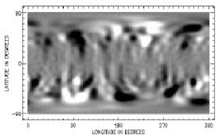
Figure 1: A map of the surface radial magnetic field of AB Dor. White represents -800G and black represents 800G. Since AB Dor is inclined at 60^∘ to the observer, Zeeman-Doppler images provide only limited information in the lower hemisphere. In order to compensate for this, we have generated this combined surface map, with the 1995 map in the upper hemisphere and the 1996 map in the lower hemisphere. The observable hemisphere of AB Dor typically shows one longitude range of predominantly positive polarity, while the remaining range of longitudes is of predominantly negative polarity. We have chosen the alignment of the 1995 and 1996 maps such that they are antisymmetric about the equator, with the predominantly positive polarity regions 180 degrees apart in longitude in the two hemispheres.

The aim of this paper is to use the Zeeman-Doppler maps of the surface magnetic field of AB Dor to extrapolate the coronal field and hence, by assuming hydrostatic equilibrium, to determine the coronal density and X-ray emission. By varying the base density and calculating the emission measure and the rotational modulation, we can determine if it is possible to reconcile the observations of high densities and high emission measures with the low rotational modulation.

2 Field extrapolation

The method of extrapolating the coronal field has been described in jardine01structure and will not be repeated in detail here. We use the source surface method pioneered by altschuler69 and a code originally developed by vanballegooijen98. Briefly, we write the magnetic field ${B}$ in terms of a flux function $\Psi$ such that $\mbox{\boldmath${B}$}=-\mbox{\boldmath${\nabla}$}\Psi$ and the condition that the field is potential ($\mbox{\boldmath${\nabla}$}\times\mbox{\boldmath${B}$}=0$) is satisfied automatically. The condition that the field is divergence-free then reduces to Laplace’s equation $\mbox{\boldmath${\nabla}$}^{2}\Psi=0$ with solution in spherical co-ordinates $(r,\theta,\phi)$

$$\Psi=\sum_{l=1}^{N}\sum_{m=-l}^{l}[a_{lm}r^{l}+b_{lm}r^{-(l+1)}]P_{lm}(\theta)e^{im\phi},$$ (1)

where the associated Legendre functions are denoted by $P_{lm}$. The coefficients $a_{lm}$ and $b_{lm}$ are determined by imposing the radial field at the surface from the Zeeman-Doppler maps and by assuming that at some height $R_{s}$ above the surface the field becomes radial and hence $B_{\theta}(R_{s})=0$. This second condition models the effect of the plasma pressure in the corona pulling open field lines to form a stellar wind. Since large slingshot prominences are observed on AB Dor mainly around the co-rotation radius which lies at $2.7R_{\star}$ from the rotation axis, we know that a significant fraction of the corona is closed out to those heights and so we set the value of $R_{s}$ to $3.4R_{\star}$.

We find that much of the corona is filled with open field lines, and will therefore be dark in X-rays. These open field lines originate in two opposite-polarity, mid-latitude regions located 180^∘ apart in longitude. The closed field volume between these two “coronal holes” forms a torus that extends almost over both poles and whose axis connects the two “open field” longitudes.

3 Calculating the density

In order to relate our model to the observations, we determine the X-ray emission from the closed field regions. As a first step, we calculate the pressure structure of the corona assuming it to be isothermal and in hydrostatic equilibrium. Hence for a stellar rotation rate $\omega$, the pressure at any point is $p=p_{0}e^{\int g_{s}ds}$ where $g_{s}=({\bf g.B})/|{\bf B}|$ is the component of gravity (allowing for rotation) along the field and

$$g(r,\theta)=\left(-GM_{\star}/r^{2}+\omega^{2}r\sin^{2}\theta,\omega^{2}r\sin\theta\cos\theta\right).$$ (2)

We note that for AB Dor, $\omega=1.4\times 10^{-4}$s^-1, a factor of 50 times greater than the corresponding solar value. At the loop footpoints we scale the plasma pressure $p_{0}$ to the magnetic pressure such that $p_{0}(\theta,\phi)=RB^{2}_{0}(\theta,\phi)$ where $R$ is a constant. The plasma pressure within any volume element of the corona is set to zero if the field line through that volume element is open. In order to mimic the effect of a high gas pressure forcing closed field lines to open up, we also investigate the effect of setting the plasma pressure to zero if the plasma pressure is greater than the magnetic pressure i.e. where $\beta>1$. From the pressure, we calculate the density assuming an ideal gas and determine the morphology of the optically thin X-ray emission by integrating along lines of sight through the corona.

Figure 2: Emission measure $\int n_{e}^{2}dV$ for an isothermal corona at a temperature of $10^{6}$K for solar maximum (solid line) and solar minimum (dotted line) as a function of the emission-measure weighted density. In each case the branching of the curves at high densities shows the amount by which the emission is reduced if field lines where the plasma pressure exceeds the magnetic pressure are assumed to have been forced open.

This technique has been used for some time now to extrapolate the coronal field of the Sun. Comparisons of the resulting morphology of the corona with LASCO C1 images [Wang et al.1997] show good agreement for much of the corona, except near the polar hole boundaries where the potential field approximation is likely to break down at the interface between open and closed field regions. wang97 found the best agreement with observations was obtained with a scaling of $p_{0}\propto B^{0.9}_{0}$. The question of the optimal scaling is one that is often addressed in the context of the heating of the solar corona (see aschwanden2001 and references therein) and indeed recent work suggests that scaling laws developed on the basis of detailed solar observations may be extrapolated to more rapidly rotating stars [Schrijver & Aschwanden2002]. Given that our intent is not to discriminate between heating models, but rather to demonstrate that the observed surface field distributions are consistent with the X-ray observations, we opt for the simplest prescription that fits the data. Our choice of $p_{0}\propto B^{2}_{0}$ ensures that regions of high field strength will emit strongly. This naturally concentrates much of the emission at high latitudes.

Figure 3: Rotational modulation of the emission measure for three different surface maps. The dashed curve is for the 1995 dataset. The other two curves are for a mixed dataset with the 1995 map in the upper hemisphere and the 1996 dataset in the lower hemisphere. In each case the relative orientation of the two maps is different. The dotted line is the case where the regions of predominantly the same polarity in each hemisphere are 180^∘ apart in longitude; the solid line is the case shown in Fig. 1 where they are at the same longitude.

Figure 4: Emission measure for the combined surface map shown in Fig. 1 with a dipole component of different strengths added.

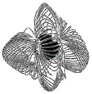
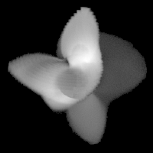
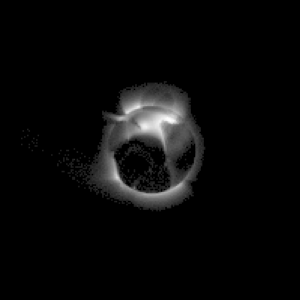
Figure 5: The effect of the coronal temperature on the emission measure. Fig. 5 shows the magnetic structure of the large-scale field based on the surface map shown in Fig. 1. The field is viewed from longitude $128^{\circ}$. Figs. 5 and 5 show the corresponding emission measure images on a squre-root stretch at temperatures of 10⁷K, and 10⁶K respectively. The corresponding emission-measure weighted densities are $4\times 10^{8}$cm^-3 and $2\times 10^{8}$cm^-3.

In order to test the model, we extrapolate the field from two solar magnetograms taken from the NSO/KP data archive, one from solar maximum (1992 Feb 1) and one from solar minimum (1996 April 8). With a source surface set to 2.5 R_⊙ and a uniform temperature of $10^{6}$K we determine the total emission measure ($\int n_{e}^{2}dV$) for a range of values of the scaling constant $R$. Although the density at the base of the corona is the parameter that we can vary with this model, this is not necessarily the density that is observed. We therefore determine the emission-measure weighted density ($\int n_{e}^{3}dV/\int n_{e}^{2}dV$) and use this as a measure of the coronal density. Fig. 2 shows the resulting emission measure for the two magnetograms. In each case, emission measures were calculated both with and without a cutoff for high pressures. This causes the branching of the curves at high densities, with the lower branch being the case where a cutoff was imposed. We do not expect this simple one-temperature model to reproduce the detailed changes in the magnitude and temperature distribution of the Sun’s X-ray emission through its cycle. Nonetheless, the overall morphology of the emission and the observed range of emission measures of $10^{49}-10^{50}$cm^-3 are easily reproduced and correspond to densities of the order of $10^{9}$cm^-3 [Peres et al.2000].

4 Modelling the corona of AB Dor

In the case of the Sun, resolved X-ray observations can be used to test field extrapolation models. For other stars however we generally have only the emission measure and the rotational modulation to give us insight into the field structure. In this section we determine the effect of the different assumptions of our model on these two quantities.

4.1 The effect of hidden flux

Flux can be undetected by the Zeeman-Doppler method if it is located in the unobservable hemisphere of the star, or in regions of the stellar surface that are dark, such as the polar cap. jardine01structure explored the effect of this hidden flux by adding to the maps of the observable hemisphere either a polar field (in the form of a global dipole) or the surface map for another year added in to the hidden hemisphere (see Fig. 1). In all these cases the structure of the field (and in particular the positions of the open field regions) is quite different. These differences are, however, unlikely to be apparent in the rotational modulation and magnitude of the X-ray emission measure which is the main observational signature of this field.

This is demonstrated in Fig. 3 which shows this rotational modulation for three different surface maps. The lowest curve comes from a surface map that has data only in the observable hemisphere. There is very little rotational modulation, since flux in the lower hemisphere which might be eclipsed as the star rotates is missing. The upper two curves show the effect of having flux in both hemispheres. In one case, the predominantly positive polarity regions in the two hemispheres are aligned, and in the other case they are 180^∘ apart in longitude (this is the case shown in Fig. 1). There is little difference in the rotational modulation of these two cases.

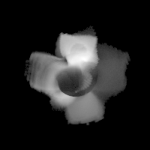
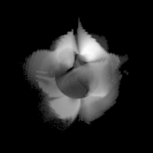
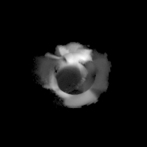
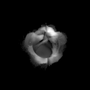
Figure 6: The effect of the coronal density on the emission measure. Shown are both emission measure images (viewed from longitudes $128^{\circ}$ and $38^{\circ}$) and the corresponding rotational modulation. All models have the same magnetic structure as Fig. 5, a temperature of 10⁷K and a cutoff imposed in the emission for $\beta>1$. The top panels are for a model with an emission-measure weighted density $n_{e}=4\times 10^{8}$cm^-3, while the bottom panels have $n_{e}=1.5\times 10^{10}$cm^-3.

jardine01structure also examined the change in field structure produced by a “pseudo-dipole” field hidden in the dark polar cap. This field is not a true dipole since the longest field lines (those that emerge from the highest latitudes on the star) extend to the source surface and so are forced to be open. As the flux in the dipolar component is increased, it has a progressively greater influence on the overall field structure until, once it dominates completely, the large-scale field is indistinguishable from the pseudo-dipole. Beyond this point, increasing the polar field strength has little effect on the field structure, but it would increase the emission measure. Since for an isothermal corona, the density scales as the plasma pressure (and hence in our model as the field strength squared) we would expect the emission measure to scale as the polar field strength to the power four. Fig. 4 shows the variation of the emission measure with the strength of a polar field added in to the combined surface map shown in Fig. 1. Adding a weak polar field ($\leq 200$G) reduces the emission measure as it forces some of the high-latitude field that was originally closed to become open. Beyond this field strength, the addition of the dipolar component increases the emission measure. Even with a polar field strength of a few kilogauss, however, the emission measure is increased by only a factor of 10. Dipolar fields stronger than this would be observable in the Zeeman maps.

Clearly, while the effect of the hidden flux is important in influencing the field topology and the location of the open field regions from which the wind may escape, the observational capabilities we have at present are not sufficient to distinguish the nature of this flux. The different cases we have examined all show rotational modulations less than around $20\%$ which is close to the observed range. While adding a dipole field could in principal give an observable change to the emission measure, the field strengths that can be hidden in the dark polar cap are not large enough to make an observable difference.

In the light of this, we keep the same field topology for the rest of this paper, using only the combined surface map shown in Fig. 1.

4.2 The effect of the coronal temperature

The coronal temperature influences the X-ray emission primarily through its effect on the density scale height. As Fig. 5 shows, at T=10⁶K the corona is much more confined than at T=10⁷K. Lowering the temperature not only lowers the overall emission level (in this case by two orders of magnitude) but it increases the rotational modulation. This increase (from $5\%$ to $12\%$) is, however, small because the regions that emit most strongly are at high enough latitudes that they are always in view. In both these cases, the magnetic structure is the same. Hence, for this low-temperature model, large loops still exist, but their summit density is much lower and hence they are not so bright in X-rays. This may of course have implications for the formation of the very massive prominences on AB Dor that are observed at some 3-5R^⋆ from the rotation axis. If the density at this height is too low, it may simply not be possible to sustain the radiative instability required to form the prominences.

4.3 The effect of the coronal density

This is perhaps the most critical parameter to examine as it is currently the subject of such debate. We have chosen a sample of base densities and calculated the total emission measure and the rotational modulation. In addition, we have explored the effect of modelling the breaking open of field lines when the gas pressure exceeds the magnetic pressure. In these cases, we imposed a cutoff in the emission (i.e. the density was set to zero) on those field lines where at any point along their length the plasma $\beta$, which is the ratio of plasma to magnetic pressure, was greater than one. This cutoff has little effect in models where the coronal temperature is low (T=10⁶K) since in this case the plasma pressure is also low. For the higher temperature models, however (T=10⁷K) it makes a more significant difference.

Fig. 6 shows emission measure images of the X-ray corona at two different densities. In both cases, there is a cutoff in the emission for those fieldlines with $\beta>1$. Also shown is the rotational modulation of the emission measure. These images show clearly that as the coronal density rises, the accompanying rise in plasma pressure forces open more field lines and so the volume of the emitting corona shrinks, even although the total emission measure is rising. This is accompanied by a slight increase in the magnitude of the rotational modulation, although it is still well within the observed range. The effect of imposing a cutoff in the emission where the plasma pressure exceeds the magnetic pressure can be seen by comparing Figs. 5 and 6. For both of these models, the viewing angle, base density and coronal temperature are the same, but in Fig. 5 there is no cutoff imposed. As a result, the emitting volume is independent of the density and pressure and the emission measure is larger. The rotational modulation is small in both cases.

In order to quantify this behaviour we have run a series of models of increasing base density and calculated the rotational modulation and emission measure. Fig. 7 shows the rotational modulation for a family of models at $T=10^{7}$K where a cutoff in the emission is imposed for $\beta>1$. The modulation is remarkably constant for a very wide range of coronal densities. It only begins to increase significantly at densities in excess of $10^{12}$cm^-3. At these densities, the plasma pressure at the loop footpoints is so large that even very low-lying loops are forced open by the plasma pressure. As a result, the rotational modulation increases steeply and the emission-measure weighted density in fact falls slightly. In the case where no cutoff was imposed (or the temperature was so low at $T=10^{6}$K that the cutoff was never needed) the rotational modulation is constant at $5\%$ for all models.

Although the rotational modulation of the emission measure varies little with the density of the emitting corona, the magnitude of the emission measure increases steeply. Fig. 8 shows the results of models at $T=10^{7}$K (solid) and $T=10^{6}$K (dashed). At each temperature, the curves branch into two: the upper branch is the case where there is no cutoff, while the lower branch shows how the emission is reduced when a cutoff is imposed. In the case where there is no cutoff in the emission, the volume of the emitting corona is independent of the density and so the emission measure essentially scales as $n_{e}^{2}$. This can be seen in the slope of the upper branches. As noted in the discussion of the rotational modulation, an attempt to increase the base density much above $10^{12}$cm^-3 actually results in a reduction of the emission-measure weighted density, as can be seen in the last few data points.

Figure 7: Rotational modulation of the emission measure as a function of the emission-measure weighted coronal density.

Figure 8: Total emission measure as a function of the emission-measure weighted coronal density. Models with isothermal coronae at 10⁶K (dashed) and 10⁷K (solid) are shown. In each case the curves have two branches. The lower branch shows the amount by which the emission is reduced if field lines where the plasma pressure exceeds the magnetic pressure are assumed to have been forced open. This simulates the opening up of field lines to form a stellar wind.

Figure 9: Density-weighted filling factor as a function of the emission-measure weighted coronal density. The corona is assumed to be isothermal at a temperature of 10⁷K. The lower branch shows the reduction in the filling factor if field lines where the plasma pressure exceeds the magnetic pressure are assumed to have been forced open.

Clearly, cutting off the emission when the plasma pressure exceeds the magnetic pressure results in the emission measure increasing less steeply with density. As the density increases, more and more field lines reach the critical plasma pressure and the emitting volume of the corona shrinks. This effect can be seen in Fig. 9 where we show the behaviour of the density-weighted filling factor $f$ which we define as

$$f=\frac{\int n_{e}^{2}dV}{\frac{4}{3}(R_{s}^{3}-R_{\star}^{3})n_{e}^{2}}.$$ (3)

This is the calculated emission measure as a fraction of the emission measure of a sphere extending to the source surface $R_{s}$ and uniformly filled with plasma at the coronal density. For our isothermal model, this filling factor simply measures the fraction of the coronal volume that is emitting. For the case where there is no cutoff in the emission, the filling factor is independent of the density and depends only on the structure of the magnetic field and particularly on the location and extent of the open field regions. For the models with a cutoff imposed, however, the filling factor falls sharply with increasing density as a smaller and smaller fraction of the corona contributes to the emission. For models calculated at a lower temperature of $10^{6}$K, the pressure scale height is smaller and this filling factor is correspondingly less ($~{}2\times 10^{-4}$) and independent of peak density. While the behaviour of this filling factor gives a useful qualitative understanding of the structure of the corona of AB Dor, the numerical values should be treated with caution since they refer only to an isothermal plasma. A true stellar corona is a multi-temperature plasma, and defining a filling factor is a much more complex issue since fine-scale structure in both temperature and density may contribute [Almleaky, Brown & Sweet1989, Judge2001]. Nonetheless, klimchuk2001 show that the commonly-used spectroscopic filling factor (similar to the one defined here) is a good measure of the fraction of the volume occupied by plasma within a narrow temperature band.

The observed range of total emission measures for AB Dor extends from $10^{52.8}-10^{53.3}$cm^-3 [Vilhu et al.2001]. On the basis of the models shown in Fig. 8 this corresponds to densities in the range $10^{9}-10^{10.7}$cm^-3. Using a model with a cutoff imposed for high-pressure fieldlines reduces this range to $10^{9.4}-10^{10.5}$cm^-3. In either case, the implied densities are high by solar standards, but span the value of $10^{10.5}$cm^-3 obtained from XMM-Newton observations [Güdel et al.2001a]. In fact a model run for a temperature of $3\times 10^{6}$K appropriate for these observations gives an emission measure of $10^{53.6}$cm^-3 for a density of $10^{10.5}$cm^-3.

5 Conclusions

While our calculation of the coronal magnetic field structure of AB Dor is based directly on the Zeeman-Doppler images, our calculation of the pressure and density structure of the corona is more model-dependent. With the very simplest of assumptions however (an isothermal plasma in hydrostatic equilibrium) we have been able to reproduce the observed emission measures, densities and rotational modulation in X-rays. The key to our ability to reconcile the high emission measures and densities with the low rotational modulation lies in the complex nature of the magnetic field. The Zeeman-Doppler images show a surface that is densely covered in flux. Extrapolating this surface field shows that the corona contains loops on all scales and with a range of field strengths. In the low-density models, the corona is very extended and so shows little rotational modulation. In the higher density models, the emitting corona is more compact, but again shows little rotational modulation since the brightest regions are at high latitudes where they are always in view as the star rotates.

6 Acknowledgements

We would like to thank Dr A. van Ballegooijen for allowing us to use his code for calculating the potential field extrapolation. The synoptic magnetic data used in this study were produced cooperatively by NSF/NOAO, NASA/GSFC, NOAA/SEL and NSO/Kitt Peak and made publicly accessible via the World Wide Web.

References

- [\citefmtAlmleaky, Brown & Sweet1989] Almleaky Y., Brown J., Sweet P., 1989, A&A, 224, 328
- [\citefmtAltschuler & Newkirk, Jr.1969] Altschuler M. D., Newkirk, Jr. G., 1969, Solar Phys., 9, 131
- [\citefmtAschwanden2001] Aschwanden M., 2001, ApJ, 560, 1035
- [\citefmtAudard et al.2001] Audard M., Behar E., Güdel M., Raassen A., Porquet D., Mewe R., Foley C., Bromage G., 2001, aanda, 365, L329
- [\citefmtBrickhouse & Dupree1998] Brickhouse N., Dupree A., 1998, ApJ, 502, 918
- [\citefmtCollier Cameron & Robinson1989a] Collier Cameron A., Robinson R. D., 1989a, MNRAS, 236, 57
- [\citefmtCollier Cameron & Robinson1989b] Collier Cameron A., Robinson R. D., 1989b, MNRAS, 238, 657
- [\citefmtCollier Cameron et al.1988] Collier Cameron A., Bedford D. K., Rucinski S. M., Vilhu O., White N. E., 1988, MNRAS, 231, 131
- [\citefmtDonati & Brown1997] Donati J.-F., Brown S., 1997, A&A, 326, 1135
- [\citefmtDonati, Henry & Hall1995] Donati J.-F., Henry G. W., Hall D. S., 1995, A&A, 293, 107
- [\citefmtDupree et al.1993] Dupree A., Brickhouse N., Doschek G., Green J., Raymond J., 1993, ApJ, 418, L41
- [\citefmtGiampapa et al.1996] Giampapa M., Rosner R., Kashyap V., Fleming T., Schmitt J., Bookbinder J., 1996, ApJ, 463, 707
- [\citefmtGüdel et al.1995] Güdel M., Schmitt J., Benz A., Elias II N., 1995, A&A, 301, 201
- [\citefmtGüdel et al.2001a] Güdel M. et al., 2001a, A&A, 365, L336
- [\citefmtGüdel et al.2001b] Güdel M. et al., 2001b, in R. Giaconni L. Stella S. S., ed, Proceedings of “X-ray astronomy 2000”. ASP conference series
- [\citefmtJardine, Collier Cameron & Donati2002] Jardine M., Collier Cameron A., Donati J.-F., 2002, MNRAS, 333, 339
- [\citefmtJeffries1998] Jeffries R., 1998, MNRAS, 295, 825
- [\citefmtJudge2001] Judge P., 2001, ApJ, 531, 585
- [\citefmtKlimchuk & Cargill2001] Klimchuk J. A., Cargill P., 2001, ApJ, 553, 440
- [\citefmtKürster et al.1997] Kürster M., Schmitt J., Cutispoto G., Dennerl K., 1997, A&A, 320, 831
- [\citefmtLim et al.1994] Lim J., White S., Nelson G., Benz A., 1994, ApJ, 430, 332
- [\citefmtMaggio et al.2000] Maggio A., Pallavicini R., Reale F., Tagliaferri G., 2000, A&A, 356, 627
- [\citefmtMewe et al.1996] Mewe R., Kaastra J., White S., Pallavacini R., 1996, A&A, 315, 170
- [\citefmtMewe et al.2001] Mewe R., Raassen A., Drake J., Kaastra J., van der Meer R., Porquet D., 2001, A&A, 368, 888
- [\citefmtPeres et al.2000] Peres G., Orlando S., Reale F., Rosner R., Hudson H., 2000, ApJ, 528, 537
- [\citefmtSchrijver & Aschwanden2002] Schrijver C., Aschwanden M., 2002, ApJ, 566
- [\citefmtSchrijver et al.1995] Schrijver C., Mewe R., van den Oord G., Kaastra J., 1995, A&A, 302, 438
- [\citefmtSiarkowski et al.1996] Siarkowski M., Prés P., Drake S., White N., Singh K., 1996, ApJ, 473, 470
- [\citefmtSingh, White & Drake1996] Singh K., White N., Drake S., 1996, ApJ, 456, 766
- [\citefmtStrassmeier1996] Strassmeier K., 1996, in Strassmeier, K.G., Linsky, J.L., eds, IAU Symposium 176: Stellar Surface Structure. Kluwer, p. 289
- [\citefmtvan Ballegooijen, Cartledge & Priest1998] van Ballegooijen A., Cartledge N., Priest E., 1998, ApJ, 501, 866
- [\citefmtVilhu et al.2001] Vilhu O., Mulhi P., Mewe R., Hakala P., 2001, A&A, 375, 492
- [\citefmtWang et al.1997] Wang Y.-M. et al., 1997, ApJ, 485, 419
- [\citefmtWhite et al.1990] White N. E., Shafer R. A., Horne K., Parmar A. N., Culhane J. L., 1990, ApJ, 350, 776
- [\citefmtYoung et al.2001] Young P., Dupree A., Wood B., Redfield S., Linsky J., Ake T., Moos H., 2001, ApJ, 555, L121