Luminosity Functions beyond the spectroscopic limit

We have developed a Monte Carlo method to compute the luminosity function of galaxies, based on photometric redshifts, which takes into account the non-gaussianity of the probability functions, and the presence of degenerate solutions in redshift. In this paper we describe the method and the mock tests performed to check its reliability. The NIR luminosity functions and the redshift distributions are determined for near infrared subsamples on the HDF-N and HDF-S. The results on the evolution of the NIR LF, the stellar mass function, and the luminosity density, are presented and discussed in view of the implications for the galaxy formation models. The main results are the lack of substantial evolution of the bright end of the NIR LF and the absence of decline of the luminosity density up to a redshift $z\sim 2$, implying that most of the stellar population in massive galaxies was already in place at such redshift.

1 Introduction

The study of galaxy formation and evolution implies the availability of statistical samples at large look-back times. At large redshifts, though, only star forming galaxies will be entering the samples obtained in the visible bands and, to be able to probe their stellar masses, observations at longer wavelengths are needed. In the last decade, deep photometric galaxy samples have become available, namely through the observations by HST of the HDF-N (Williams et al. williams (1996)) and HDF-S (Casertano et al. casertano (2000)), which have been coordinated with complementary observations from the ground at near-infrared (NIR) wavelengths (Dickinson et al.dick (2000); da Costa et al. dacosta (1998)). At the same time, reliable photometric redshift techniques have been developed, allowing estimates of the distances of faint galaxies for which no spectroscopic redshifts can be obtained nowadays, even with the most powerful telescopes (e.g. Connolly et al.  con (1997); Wang et al. wan (1998); Giallongo et al. gia (1998); Fernández-Soto et al. fsoto (1999); Arnouts et al. arnouts (1999); Furusawa et al. furu (2000); Rodighiero et al. rodighiero (2001); Le Borgne & Rocca-Volmerange leborgne (2002); Bolzonella et al. hyperz (2000) and the references therein).

One of the main issues for photometric redshifts is to study the evolution of galaxies beyond the spectroscopic limits. The relatively high number of objects accessible to photometry per redshift bin allows to enlarge the spectroscopic samples towards the faintest magnitudes, thus increasing the number of objects accessible to statistical studies per redshift bin. Such slicing procedure can be adopted to derive, for instance, redshift distributions, luminosity functions in different bands, or rest-frame colours as a function of absolute magnitudes, among the relevant quantities to compare with the predictions derived from the different models of galaxy formation and evolution. This approach has been recently used to infer the star formation history at high redshift from the UV luminosity density, to analyse the stellar population and the evolutionary properties of distant galaxies (e.g. SubbaRao et al. subba (1996); Gwyn & Hartwick gwyn (1996); Sawicki et al. sawicki (1997); Connolly et al. con (1997); Pascarelle et al. pascarelle (1998); Giallongo et al. gia (1998); Fernández-Soto et al. fsoto (1999); Poli et al. poli (2001)), or to derive the evolution of the clustering properties (Arnouts et al. arnouts (1999); Magliocchetti & Maddox maglio (1999), Arnouts et al. arnouts2 (2002)).

We have developed a method to compute luminosity functions (hereafter LFs), based on our public code hyperz to determine photometric redshifts (Bolzonella et al. hyperz (2000)). This original method is a Monte Carlo approach, different from the ones proposed by SubbaRao et al. (subba (1996)) and Dye et al. (dye (2001)) in the way of accounting for the non-gaussianity of the probability functions, and specially to include degenerate solutions in redshift. In this paper we present the method and the tests performed on mock catalogues, and we apply it specifically to derive NIR LFs and their evolution on the HDF-N and HDF-S.

The NIR luminosity is directly linked to the total stellar mass, and barely affected by the presence of dust extinction or starbursts. According to Kauffmann & Charlot (kauff (1998)), the NIR LF and its evolution constitute a powerful test to discriminate between the different scenarios of galaxy formation, i.e. if galaxies were assembled early, according to a monolithic scenario, or recently from mergers. The theoretical NIR LFs derived by Kauffmann & Charlot exhibit a sharp difference between the two models at redshifts $z>1$. The PLE models foresee a constant bright-end for the LF, whereas hierarchical models are expected to undergo a shift towards faint magnitudes with increasing redshift. In this paper we compare the theoretical predictions with the observations on the HDFs, in order to extend the analysis performed from spectroscopic surveys (Glazebrook et al. glaze (1995), Songaila et al. songaila (1994), Cowie et al. cowie2 (1996)) up to $z\sim 2$. The comparison between the present NIR LF results and a similar study in the optical-UV bands, obtained with the same photometric redshift approach (Bolzonella et al. Paper II, in preparation), could provide with new insights on the galaxy formation scenario.

The plan of this paper is the following. Section 2 gives a brief description of the photometric catalogues used to select the samples, their properties being discussed in Sect. 3. In Sect. 4 we describe the technique conceived to compute the luminosity functions using the hyperz photometric redshift outputs, and the test of the method through mock catalogues. The results obtained on the HDFs near-infrared LF are presented and discussed in Section 5, together with the Luminosity Density and the Mass Function derived from them. The implications of the present results on the galaxy formation models are discussed in Sect. 6, and the main results are summarized in Sect. 7.

Throughout this paper we adopt the cosmological parameters $\Omega_{0}=1$, $\Omega_{\Lambda}=0$, when not differently specified. Magnitudes are given in the AB system (Oke oke (1974)). Throughout the paper, the Hubble Space Telescope filters F300W, F450W, F606W and F814W are named $U_{300}$, $B_{450}$, $V_{606}$ and $I_{814}$ respectively.

2 Photometric catalogues

The HDF-N (Williams et al. williams (1996)) and HDF-S (Casertano et al. casertano (2000)) are the best data sets to which the photometric redshift techniques can be applied, because of the wavelength coverage extending from the $U_{300}$ to the $K_{s}$ bands through a combination of space and ground based data, and of the accurate photometry available. Table 1 gives the characteristics of the filters involved.

For the HDF-N we adopted the photometric catalogue provided by Fernández-Soto et al. (fsoto (1999)). These authors used the SExtractor (Bertin & Arnouts bertin (1996)) package and detected objects in the $I_{814}$ image. The final catalogue consists of a total of $1067$ galaxies (after exclusion of known stars) in $5.31$ arcmin². The reference aperture used to measure the fluxes in the different bands is defined by the threshold isophote on the $I_{814}$ image. This catalogue is divided in 2 zones: the deepest one (Z1) consists of 946 objects in $3.92$ arcmin² and it has been limited to $I_{814}(AB)\leq 28$ (in “best” magnitudes, see SExtractor user manual), the shallowest one (Z2, including field edges and the planetary camera) contains 121 objects to $I_{814}(AB)\leq 26$, in an area of $1.39$ arcmin².

For the HDF-S we adopted the photometric catalogue prepared by Vanzella et al. vanzella (2001) and available on the web. The catalogue contains $1611$ objects, detected in the $V_{606}+I_{814}$ image and with magnitudes measured inside a variable aperture suited to compute photometric redshifts. The NIR imaging has been carried out with the near-infrared spectrometer/imager VLT-ISAAC and the photometry has been measured taking into account the different PSF of NIR images.

Table 1: Characteristics of photometric data used in this paper: effective wavelength, bandpass and AB conversion (conv${}_{\rm AB}=m_{\rm AB}-m_{\rm Vega}$) for the different filters, and limiting magnitudes in the HDF-N and HDF-S (see text).

Filter	$\lambda_{\rm eff}$	$\Delta\lambda$	convAB	$m_{\rm lim}^{\rm HDF-N}$	$m_{\rm lim}^{\rm HDF-S}$
	Å	Å	mag	mag	mag
$U_{300}$	3010	854	1.381	29.0	28.3
$B_{450}$	4575	878	-0.064	28.5	28.5
$V_{606}$	6039	1882	0.132	28.5	28.5
$I_{814}$	8010	1451	0.439	28.0	28.0
$J$	12532	2651	0.937	25.5	25.8
$H$	16515	2903	1.407	25.0	25.0
$K_{s}$	21638	2724	1.871	25.0	25.3

3 Sample properties

3.1 Photometric Redshifts

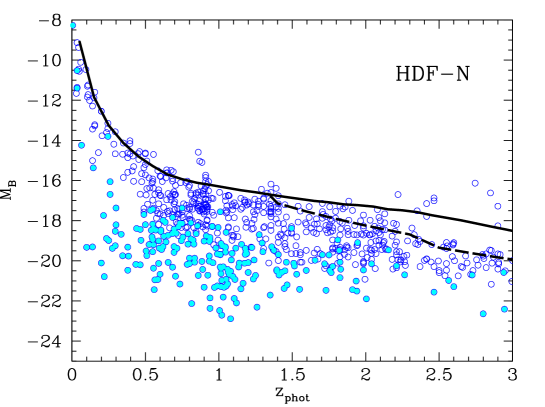
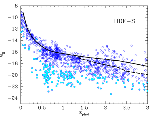
Figure 1: Absolute magnitude in the $B$-band as a function of photometric redshift in the HDF-N and HDF-S for objects with $B_{450}\leq 28.5$. The filled dots represent the subsample with $K_{s}\leq 24$, used to estimate the luminosity functions in Section 4. The solid lines mark the limiting absolute magnitude computed using the apparent limiting magnitude of the sample in the $B_{450}$ band, and the mean $k$-correction over a mix of spectral types. The dashed lines display the same result when using the limiting magnitudes for the NIR filters.

To compute photometric redshifts, we converted the fluxes $f_{\nu}$ into AB magnitudes, assigning the magnitude value of $99$ (corresponding to an undetected object in our photometric redshift scheme) in case of negative fluxes, negative error fluxes, or $S/N=f_{\nu}/\Delta f_{\nu}<1$. Moreover, we added in quadrature a photometric error of $0.02$ magnitudes in all filters, to account for systematics in the zeropoints.

Then, we applied the public code hyperz to compute the photometric redshifts of galaxies in the HDF-N and HDF-S. A full description of the technique and the analysis of the performances on the HDFs can be found in Bolzonella et al. (hyperz (2000)). Here we only recall that an interesting characteristic of the hyperz code is the possibility of computing probability functions in the redshift space. We will make full use of this facility to derive the LFs.

A full description of the different parameters used by hyperz can be found in the User’s Manual of the code, available on the web pages. The most relevant parameters used here are the following:
– The limiting magnitudes applied in case of undetected objects are given in Table 1. We choose $P(<m)=0.8$ in the cumulative histograms to set the adopted limiting magnitudes, which roughly correspond to objects with a $S/N\sim 1$.
– We used Calzetti’s (calzetti (2000)) law to produce reddened templates, with $A_{V}$ ranging from $0$ to $1.2$ magnitudes.
– The Lyman forest blanketing is modelled according to the standard prescriptions of Madau (madau (1995)), without variations along the different lines of sight.
– As galaxy template set we selected the $5$ “standard” SEDs built using the GISSEL98 library by Bruzual & Charlot (bruzual (1993)), with solar metallicity; the CWW SEDs were not considered because they are redundant.
– The range of absolute magnitudes $M_{B}$ constraining the allowed solutions is $[-28,-9]$.

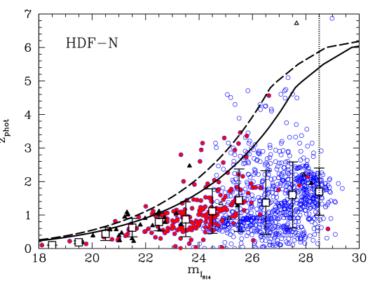
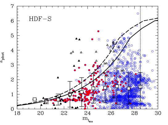
Figure 2: Hubble diagram for objects in the HDF-N and HDF-S samples. Filled symbols represent the subsample with $K_{s}\leq 24$. Triangles show the objects for which $P(z_{\rm phot})=0$ everywhere. Dashed and solid lines display the location on this diagram of a local $L^{*}$ galaxy, with cosmological parameters ($\Omega_{0}=1$, $\Omega_{\Lambda}=0$) and ($\Omega_{0}=0.3$, $\Omega_{\Lambda}=0.7$) respectively, with $H_{0}=50\,{\rm km\,s^{-1}\,Mpc^{-1}}$. The vertical dotted line marks the $I_{814}=28.5$ magnitude at which the signal-to-noise ratio is $S/N=3$. The mean redshift and the $1\sigma$ dispersion have also been plotted.

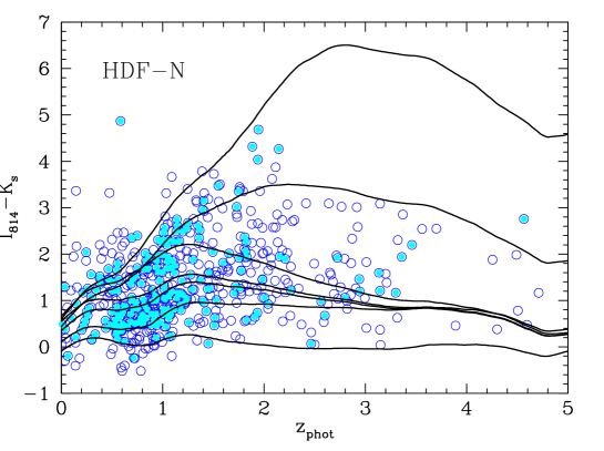
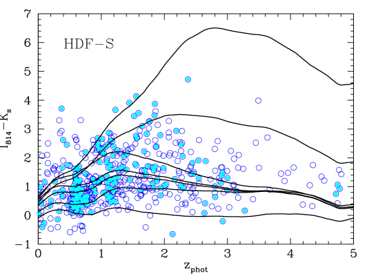
Figure 3: Colour $I_{814}-K_{s}$ as a function of photometric redshift, compared to the predictions for different synthetic SEDs. From top to bottom: Elliptical galaxy of fixed $10$ and $5$ Gyr age, evolving E, Sa, Im, and Im of fixed $1$ and $0.1$ Gyr age. Empty dots illustrate the sample with $K_{s}\leq 26$ in the HDF-N and HDF-S samples, corresponding to $S/N=1$, whereas filled dots represent objects with $K_{s}\leq 24$, i.e. with $S/N\geq 3$. The observed colours are enclosed in the limits of colours foreseen from the synthetic SEDs.

A comparison between the photometric and spectroscopic redshifts has been shown in Bolzonella et al. (hyperz (2000)). Here we assume that galaxies in the photometric sample will follow the same behaviour, i.e. the same dispersion around the true values. Beyond $I_{814}=25$ our spectroscopic knowledge falls dramatically. Very few objects are available to calibrate the photometric redshifts in this domain, and so larger discrepancies are always possible. Nonetheless, these objects will remain beyond the spectroscopic limits till the arrival of larger telescopes in the future, and photometric redshifts are presently the only available tool to study them.

We used the results of the photometric redshift estimate to examine some properties of the sample and to give an estimate of the evolution in the samples.

Figure 1 displays the absolute magnitude in the $B$-band, obtained as standard output of hyperz, as a function of the photometric redshift for objects with $B_{450}\leq 28.5$. The thick solid line represents the limiting absolute magnitude computed for a $B=28.5$ object and a mean $k$-correction computed over a mix of spectral types, with the method explained below in Sect. 4.3. For comparison, the thick dashed lines show the same result when using the limiting magnitudes given in Table 1 for the NIR filters. It is worth to remark the sequence of theoretical absolute magnitudes, in agreement with the observational limits, obtained without imposing stringent constraints in $M_{B}$.

In Fig. 2 we plot the observed $I_{814}$ magnitudes versus the photometric redshift, viz the Hubble diagram. The mean redshift per magnitude bin is also shown, with its $1\sigma$ dispersion. The faintest objects are also the farthest ones, as we expect for an expanding universe. The position on this Hubble diagram of a local $L^{*}$ galaxy is also shown for comparison, for the two sets of cosmological parameters used in this paper. In the HDF-S there are some objects well above the $L^{*}$ lines: most of them are objects with $P(z_{\rm phot})=0$, shown as triangles. Nearly half of these objects are classified by SExtractor as stars in the Vanzella et al. (vanzella (2001)) catalogue. When we fit their SEDs with stellar templates (Pickles pickles (1998)) and quasar spectra (according to the method described by Hatziminaoglou et al. evanthia (2000)), only one of these objects has colors fully consistent with a highly reddened star. In all the other cases, these objects are not well fitted neither with the standard SEDs for galaxies nor with the stellar or quasar templates. Thus, we have no reason to exclude them when computing LFs.

The inspection of these two figures indicates that the statistical properties of the photometric redshift samples display the expected behaviour. According to our previous simulations, aiming to reproduce the properties of the HDFs (Bolzonella et al. hyperz (2000)), the redshift distribution beyond the spectroscopic limits can be considered as reliable.

In Fig. 3 we plot the apparent colour $I_{814}-K_{s}$ versus the photometric redshift, as well as the colours computed from the synthetic SEDs of different types: from top to bottom, an Elliptical galaxy at fixed ages of $10$ Gyr and $5$ Gyr, evolving E, Sa, Im, Im of fixed $1$ Gyr and $0.1$ Gyr age. A few objects redder than old ellipticals seem to be present at $z<1$ in both fields. Also, a group of objects with $I_{814}-K_{s}>2.6$ and $1\la z\la 2$ is detected: these objects are EROs according to the usual criteria (e.g. Cimatti et al. cimatti (1999); Scodeggio & Silva scodeggio (2000); Moriondo et al. mori (2000)).

3.2 Redshift distribution

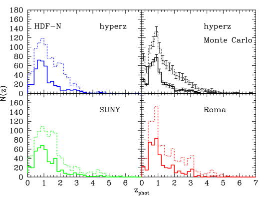
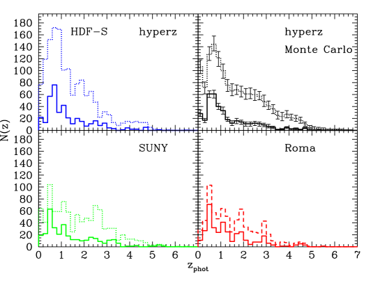
Figure 4: Redshift distributions obtained for the $I_{814}$ selected samples in the HDF-N and HDF-S by different authors. Left panel: $N(z)$ in the HDF-N obtained using the SUNY catalogue by hyperz, hyperz with a Monte Carlo method, Fernández-Soto et al. (fsoto (1999)) and Fontana et al. (fonta1 (2000)), with limiting magnitudes of $I_{814}=28.5$ (dotted line) and $I_{814}=26$ (solid line). Right panel: $N(z)$ in the HDF-S, with the same two limiting magnitudes. Fontana et al. (fonta1 (2000)) used the SUNY catalogue, limiting their analysis to $I_{814}=27.5$ (dashed line).

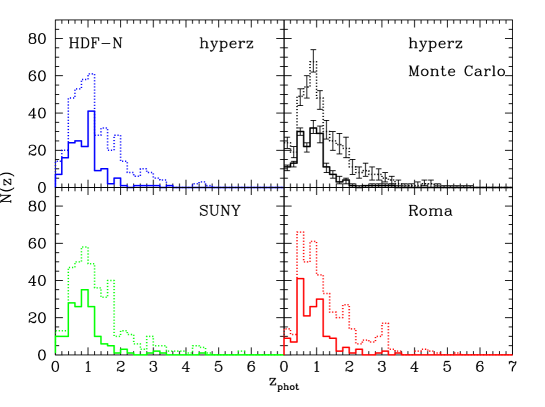
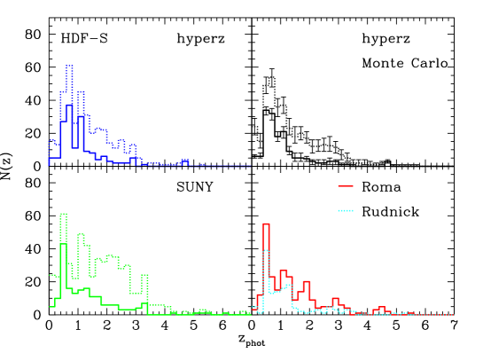
Figure 5: Redshift distributions obtained for the $K_{s}$ selected subsamples in the HDF-N and HDF-S by different authors. Left panel: $N(z)$ in the HDF-N obtained using the SUNY catalogue by hyperz, hyperz with a Monte Carlo method, Fernández-Soto et al. (fsoto (1999)) and Fontana et al. (fonta1 (2000)) with two limiting magnitudes: $K_{s}\leq 25$ (dotted line) and $K_{s}\leq 23.5$ (solid line). Right panel: the same in the HDF-S. In the lower right panel the solid line represents the $N(z)$ at $K_{s}\leq 23.5$ obtained by Fontana et al. (fonta1 (2000)) and the dotted line the $N(z)$ at the same limit by Rudnick et al. (rudnick (2001)).

Figure 4 shows the redshift distributions, as obtained from the photometric redshift computation, for the HDFs catalogues. We have compared our result on the HDF-N with the redshift distributions obtained by Fernández-Soto et al. (fsoto (1999), SUNY group) and Fontana et al. (fonta1 (2000), Roma group), using the same catalog (see Section 2). In the HDF-S, we compared our redshift distribution, obtained with the catalogue by Vanzella et al. (vanzella (2001)) with the $N(z)$ computed using the SUNY catalogue by Fernández-Soto et al.  (fsoto (1999)) and Fontana et al. (fonta1 (2000)). We have also computed a median redshift distribution, obtained with the Monte Carlo method we applied to estimate the luminosity function, and detailed in Section 4.2. This redshift distribution takes into account the probability functions of individual objects, in such a way that objects will be scattered in their allowed range of photometric redshifts, according to their $P(z_{\rm phot})$. Objects with flat $P(z_{\rm phot})$ will spread over a wide range of $z_{\rm phot}$, whereas objects with narrow $P(z_{\rm phot})$ will be always assigned to a redshift close to the best fit one. We show the result of 100 iterations, represented by the median and the error bars, computed as 10% and 90% of the values distribution in each redshift bin.

Considering the fainter sample of the HDF-N presented in the left panel of Figure 4, the Kolmogorov-Smirnov test shows that the hyperz and SUNY distributions are compatible, whereas the hyperz and Roma distributions are not. We reject the hypothesis that two distributions were issued from the same parent distributions when the significance level is lower than a conservative value of 1%. Using the same criterium, the median $N(z)$ computed with the hyperz-Monte Carlo method is compatible with both the SUNY and the Roma distributions. At $I_{814}\leq 26$, the KS test shows that each $N(z)$ is consistent with the others.

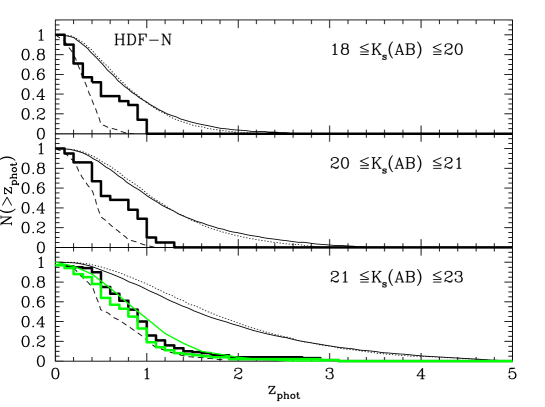
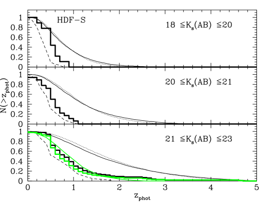
Figure 6: Cumulative redshift distribution in the $K_{s}$ band selected samples in HDF-N and HDF-S obtained with the Monte Carlo method (thick solid lines), compared to the theoretical expectations by Kauffmann & Charlot (kauff (1998)): solid and dotted lines correspond to $\Omega_{0}=1$ and $\Omega_{0}=0.2$ PLE models with null cosmological constant, whereas dashed lines correspond to their hierarchical galaxy formation model based on a $\Omega_{0}=1$ cosmology. The $3$ apparent $K_{s}$ magnitude bins roughly correspond to the original ones used by Kauffmann & Charlot (kauff (1998)). The light gray cumulative histogram in the lower panels represents $N(>z)$ for the sample with $K_{s}<23$, whereas the light gray continuous line is the theoretical expectation at the same limiting magnitude computed by Fontana et al. (fontana (1999)) for a hierarchical model based on a $\Lambda$CDM cosmology.

In the HDF-S, we show the comparison of $N(z)$ for the same two limiting magnitudes, $I_{814}\leq 28.5$ and $I_{814}\leq 26$. Fontana et al. (fonta1 (2000)) selected their subsample imposing $I_{814}\leq 27.5$ (dashed line). The KS test for the subsample with $I_{814}\leq 28.5$ shows that the distributions are not drawn from the same parent distribution, but considering the bright subsample with $I_{814}\leq 26$ the distributions are fully consistent each other, even if they are obtained from different photometric catalogues.

In Figure 5 we show the same comparison carried out for the $K_{s}$-band selected subsample we used in the following of this paper. We have analysed the distributions obtained when selecting objects with $K_{s}\leq 25$ and $K_{s}\leq 23.5$. In the HDF-N the agreement among the different $N(z)$ distributions is remarkable: by means of the Kolmogorov-Smirnov test we obtain that we can reject the possibility that the distributions were drawn from different parent distributions with a confidence level ranging from $23$% (minimum) and $70$% (maximum) at $K_{s}\leq 25$, and a probability ranging from $41$% to $100$% at $K_{s}\leq 23.5$.

In the HDF-S the same comparison shows that the hyperz and SUNY distributions are not compatible, even choosing the conservative value of $1$% for the confidence level, whereas the hyperz and Roma results are marginally consistent. On the other hand, the redshift distributions of the bright subsample show a better agreement, with probabilities in each case larger than the chosen limit, even if the catalogues are different, in particular in the NIR dataset. In the lower right panel we also show the redshift distribution obtained by Rudnick et al. (rudnick (2001)) for a sample limited to $K_{s}\leq 23.5$ and a catalogue built by these authors using ISAAC-VLT images. Also in this case we found that the redshift distributions are compatible. Even considering the subsample with $K_{s}\leq 24$, i.e. the limit chosen computing LFs, the redshift distributions are in general consistent.

In conclusion, some small differences are observed in the redshift distribution when using different methods, mostly affecting the faintest samples, whereas the results are compatible for the bright ones. At faint limits in magnitude, the redshift distribution obtained with the hyperz-Monte Carlo method avoids introducing spurious features, and it makes the relevant $N(z)$ distributions compatible. At brighter limits, by means of the comparison with the other photometric redshift estimates, we have shown that the results are consistent and characterized by a high quality in the redshift determination. The differences among different authors become very smooth when the Monte Carlo approach is used; this procedure allow us to compute reliable LFs in Sect. 5.

3.3 Cumulative redshift distribution

Kauffmann & Charlot (kauff (1998)) argued that the cumulative redshift distribution in the $K$-band can be used as a test for the scenarios of galaxy formation. In Fig. 6 we have compared our data with the theoretical expectations given by Kauffmann & Charlot (kauff (1998)), in the case of monolithic (PLE) and hierarchical galaxy formation scenarios. The original $K$-band magnitude bins have been shifted by $\sim 2$ magnitudes to match the AB magnitudes used here. The fraction of galaxies at high redshifts is much larger in the case of the PLE models than in the hierarchical scenario. The observed HDFs cumulative redshift distribution lie between the two models and, in any case, it is always below the predictions of the PLE models. This result was already pointed out by Kauffmann & Charlot (kauff (1998)), when comparing their predictions with the results found with the Songaila et al. (songaila (1994)) and Cowie et al. (cowie2 (1996)) samples, in the two brightest magnitude bins. The present results on the HDFs extend this trend towards the faintest magnitude bins. However, this results must be considered with caution, mainly because of the small size of the surveyed fields and uncertainties affecting the models. For instance, Kauffmann & Charlot derived their PLE model from the $B$-band LF. The expectations derived from monolithic and hierarchical scenarios should be more compatible in the forthcoming new generation of models (Pozzetti, private communication). On the other hand, expectations derived by Fontana et al. (fontana (1999)) for a hierarchical model in the framework of a $\Lambda$CDM cosmology seem to be in good agreement with the HDFs data. Due to the models uncertainties affecting the comparison of cumulative redshift distributions, we applied the more powerful test on the $K$-band LF proposed by Kauffmann & Charlot (kauff (1998)), whose results are shown in Sect. 5.

4 Luminosity Functions

The Luminosity Function represents the number of objects per unit volume with luminosities in the range $[L,L+dL]$. Differently from galaxy counts, distances are involved in the LF computation, where the intrinsic luminosities are considered rather then the apparent ones (except the LFs of objects belonging to a unique structure, like galaxy clusters). This characteristic makes the LF an important cosmological test, containing much more information than galaxy counts.

The LFs are of crucial importance in the description of sample statistical properties in observational cosmology. The LF can measure the amount of luminous matter in the universe, depending on the cosmological parameters. Moreover, the analysis of its characteristics and its evolution provides fundamental insights on the galaxy evolution mechanisms and can constrain the formation epoch. Studying the LFs in a wide range of absolute magnitudes is a necessity to understand the galaxy formation process. To attain this goal, more and more fainter apparent magnitudes must be reached.

4.1 LF estimators

We applied three different methods to estimate the LF: the $1/V_{\rm max}$, the $C^{-}$ and the STY methods. Willmer (willmer (1997)) and Takeuchi et al. (take (2000)) have recently reviewed and compared these estimators.

The $1/V_{\rm max}$ is the so-called classical method, first published by Schmidt (schmidt (1968)), and detailed later by Felten (felten (1976)). It was conceived for quasars, as many of the other LF estimators, but it is extensively applied in the galaxy LF computation:

$$V_{\rm max}=\int_{\min(z_{2},z_{\rm max})}^{\max(z_{1},z_{\rm min})}\frac{dV}{dz}\,dz$$ (1)

where $V_{\rm max}$ is the minimum comoving volume in the survey in which the galaxy $i$ with absolute magnitude $M_{i}$ remains observable, given $z_{1}$ and $z_{2}$, the redshift range of the survey. It is a non-parametric method, i.e. it does not assume a shape for the LF. One of the advantages of this method is its simplicity. Moreover, it is a non-parametric estimator and thus it gives the shape and the normalization at the same time. Also, it is an unbiased estimator of the source density. Of course, there are also some shortcomings. First of all, the $1/V_{\rm max}$ estimator is very sensitive to density fluctuations, especially in pencil beam surveys. Furthermore, one loses information on where in the magnitude bin a galaxy is located, but for small bins ($dM$) it is a reasonable estimate.

The $C^{-}$ method was introduced by Lynden-Bell (lynden (1971)); the original technique was simplified and developed by Chołoniewski (cholo (1987)) in such a way as to compute simultaneously the shape of the LF and the density. We adopted the Chołoniewski approach: the observed distribution of galaxies is assumed to be separable in its dependences on the absolute magnitude $M$ and the redshift $z$. As the $1/V_{\rm max}$ estimator, this method is non parametric, but it has the advantage of being insensitive to density inhomogeneities. SubbaRao et al. (subba (1996)) realized a modified version of this method, to take into account a continuum distribution of redshifts arising from the photometric redshift computation. We discuss this case later.

We also applied the STY method proposed by Sandage, Tammann & Yahil (sty (1979)). This estimator uses a maximum likelihood technique to find the most probable parameters of an analytical LF $\phi(M)$, in general assumed to be the Schechter function:

$$\phi(L)\,dL=\phi^{*}\left(\frac{L}{L^{*}}\right)^{\alpha}\exp\left(-\frac{L}{L^{*}}\right)\,d\!\left(\frac{L}{L^{*}}\right)\>,$$ (2)

that, transformed into magnitudes, becomes:

$$\phi(M)\,dM = 0.4\ln(10)\phi^{*}10^{-0.4(M-M^{*})(\alpha+1)}\times$$

$$\exp[-10^{-0.4(M-M^{*})}]\,dM\>.$$ (3)

Because the data are not binned, the method takes advantage of all the information in the sample. Imposing a functional shape, we cannot test if the assumed $\phi(M)$ is a good representation of data. Then the non-parametric methods allow to plot the data points and the STY estimator can be used to search for the better parametrization. The unknown parameters of equations 2 and 3 are the normalization $\phi^{*}$, the faint end slope $\alpha$, that assumes negative values, and the characteristic luminosity $L^{*}$ or magnitude $M^{*}$, that marks the separation between the exponential law prevailing in the bright part of the LF and the power law with index $\alpha$ dominant in the faint end. All these parameters can depend on the morphological type of galaxies under consideration. Several methods have been conceived to compute in an unbiased way the mean galaxy density and thus the parameter $\phi^{*}$. A detailed discussion of the density estimators can be found in Davis & Huchra (davis (1982)) or in Willmer (willmer (1997)).

Davis & Huchra (davis (1982)) derived a minimum variance estimator:

$$\bar{n}=\frac{\sum_{i=1}^{N}N_{i}(z_{i})\,w(z_{i})}{\int_{z_{1}}^{z_{2}}s(z)\,w(z)\,\frac{dV}{dz}\,dz}$$ (4)

where $N_{i}$ is the number of galaxies at $z=z_{i}$ (in general $N_{i}=1$, but it can take different values if galaxies are divided in redshift bins), whereas $w(z_{i})$ are the weights. The estimator called $n_{3}$ by Davis & Huchra (davis (1982)) can be derived from equation 4 by taking $w(z_{i})=1$:

$$n_{3}=\frac{N}{\int_{z_{1}}^{z_{2}}s(z)\,\frac{dV}{dz}\,dz}\>.$$ (5)

Here all the observed galaxies are equally weighed and then the estimator is quite stable, but it is affected by large scale inhomogeneities: if $\left<V/V_{\rm max}\right>>0.5$, the deduced value of $n_{3}$ can be overestimated.

4.2 Beyond the spectroscopic limit: the Monte Carlo approach

One of the problems in the study of LFs is the availability of extended samples, in terms of the number of galaxies involved in such samples, in the range of magnitudes attained (to study in detail the faint-end behaviour) and in large redshift domains (to study the evolution beyond $z\simeq 1$). However, such a sample is not easy to acquire in spectroscopic surveys, and has not yet been obtained.

A viable alternative solution is the use of the deeper and faster photometric surveys, which allow to use photometric redshifts instead of spectroscopic ones. A spectroscopic subsample is anyhow recommended, to calibrate and check photometric redshifts. A suitable survey according to these requirements is, once more, the HDFs. Different groups put a particular effort in the attempt to compute the LF of HDF-N (Gwyn & Hartwick gwyn (1996); Sawicki et al. sawicki (1997); Mobasher et al. moba2 (1996); Takeuchi et al. take (2000)).

Up to now, the approaches used to compute the Luminosity Functions by means of the photometric redshift technique, in the HDF-N or other fields, can be summarized as follows:

• the photometric redshift is assumed to be the true redshift of the galaxy, i.e. $z_{\rm phot}=z_{\rm true}$ (Gwyn & Hartwick gwyn (1996); Sawicki et al. sawicki (1997); Mobasher et al. moba2 (1996); Takeuchi et al. take (2000));

• for each object, a smooth distribution of redshifts around $z_{\rm phot}$ is considered, with a Gaussian probability function $P(z)$. The rms of the Gaussian distribution can be either a fixed value or a value depending on the apparent magnitude of the galaxy under consideration. In this case, the rms is derived from the expectations obtained from the analysis of the spectroscopic subsample. The smoothed redshift can be used in different ways: SubbaRao et al. (subba (1996)) conceived a modified version of the $C^{-}$ method to account for a continuous distribution of redshifts around $z_{\rm phot}$. Liu et al. (liu (1998)) obtained an estimate of the LF using the $1/V_{\rm max}$ method and attributing a series of fractional contributions to the luminosity distribution in the redshift space around $z_{\rm phot}$. Dye et al. dye (2001) used the Gaussian distribution to realize a series of Monte Carlo iterations, where the value of each $z_{\rm phot}$ is chosen randomly according to the Gaussian distribution.

These approaches are subject to some shortcomings, due to the nature of the photometric redshift technique itself. First, the photometric redshift is only an estimate of the true redshift, and then we can only suppose $z_{\rm phot}\approx z_{\rm true}$. Second, in most cases the probability distribution as a function of redshift, $P(z)$, cannot be assimilated to a Gaussian function, because degeneracies and uncertainties produce complex distribution functions, often with the presence of several distinct peaks. These features of the photometric redshift estimate lead to different distances $d_{L}$, absolute magnitudes $M$, volumes $V_{\rm max}$ and also to different $k$-corrections, because in general the spectral type of the best fit at a fixed redshift can be different from the best fit type of the surrounding redshift steps. Then, all these details about the photometric redshift technique must be taken into account when computing the luminosity functions of galaxies belonging to a photometric survey.

To compute the LFs in the HDF-N and HDF-S, we adopted a Monte Carlo approach, different from the Dye et al. (dye (2001)) method in the way of accounting for the non-gaussianity of the photometric redshift errors. Specifically, to assign the photometric redshift used in each iteration of the LF estimate, we build the cumulative function $P_{\rm cum}(z)$ from the $P(z)$, as described in Fig. 7. During each Monte Carlo iteration, for every galaxy we randomly select a number between $0$ and $1$, corresponding to a value of the redshift $z_{\rm prob}$ that we assign to the considered galaxy. The probability of obtaining a given value of $z_{\rm prob}$ is related to the $P(z)$ distribution: when the $P_{\rm cum}(z)$ remains horizontal, it means that the $\chi^{2}$ probability relative to those redshifts is near to $0$, and then it is almost impossible to select them by choosing a number in the interval $[0,1]$. Viceversa, vertical regions of the $P_{\rm cum}(z)$ curve correspond to very likely values of the photometric redshift.

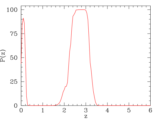
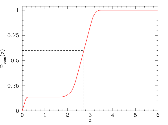
Figure 7: An example of the procedure to select the photometric redshift randomly and according to the probability distribution of the object. Left: The function $P(z)$ as computed by hyperz, renormalized to the maximum value. Right: The corresponding cumulative probability function. A random number between $0$ and $1$ is drawn. The value of $z_{prob}$ is computed by linear interpolation between the two redshift steps bracketing the value of the cumulative function equal to the random number.

Proceeding in this way, we use all the informations contained in the .log_phot file produced as output by hyperz, we take into account the existence of multiple solutions, and we are able to compute the correct $k$-corrections, knowing all the characteristics of the best fit SED at $z=z_{\rm prob}$, i.e. the associated spectral type, age and $A_{V}$.

The final data points of the LF or its fitting parameters will be evaluated by means of the median over many Monte Carlo realizations. The errors will be immediately found after sorting, by locating the values $x_{k}$ whose indexes $k$ correspond to the assigned probability. In this way we can compute the confidence intervals at different levels.

Another possibility to take into account the uncertainties and the information contained in the photometric redshift procedure, is the method described by Arnouts et al. (arnouts (1999)): they performed Monte Carlo simulations to test the effect of the photometric errors on redshift estimates. They assigned a random magnitude according to the photometric rms and verified if the changes of redshift could affect the statistics inside the redshift slices they used to divide the sample. We chose not to follow this approach, because the degeneracy among different parameters can lead to a smoothed $P(z)$, even when the photometric errors are small. In the procedure followed by Arnouts et al. (arnouts (1999)), the presence of secondary and significant peaks in $P(z)$ is not taken into account.

In the following, we adopt a cosmological model with parameters $\Omega_{0}=1$, $\Omega_{\Lambda}=0$ to facilitate the comparison of our LF results with other surveys. We compute the LFs also for the fashionable cosmological model $\Omega_{0}=0.3$, $\Omega_{\Lambda}=0.7$.

4.3 $k$-corrections

Usually, $k$-corrections in redshift surveys are computed from spectra at $z=0$, after attributing a spectro-morphological type to each object (e.g. Lilly et al. lilly (1995); Loveday et al. loveday2 (1999)). When it is impossible to separate galaxy types, a statistical $k$-correction can be computed considering a mix of morphological types (e.g. Zucca et al. zucca (1997)). The SED fitting technique used to determine photometric redshifts allows to compute a well suited $k$-correction for each object, obtained directly from the best fit SED.

The absolute magnitude of an object at redshift $z$, in a given filter $M_{\lambda}$ is:

$$M_{\lambda}=m_{\lambda}-5\log d_{L}-25-k_{\lambda}(z)\>,$$ (6)

where $d_{L}$ is the luminosity distance in Mpc, $m_{\lambda}$ is the apparent magnitude, and $k_{\lambda}(z)$, the $k$-correction, is defined by:

$$k_{\lambda}(z) = M_{\lambda}(z,t_{0})-M_{\lambda}(0,t_{0})$$ (7)

$$= 2.5\log\frac{\int f(\lambda,t_{0})R(\lambda)\,d\lambda}{\int f(\frac{\lambda}{1+z},t_{0})R(\lambda)\,d\lambda}+2.5\log(1+z)\>.$$

Here $t_{0}$ is the time corresponding to the present epoch ($z=0$); therefore, the $k$-correction is a pure geometrical correction which transforms the observed magnitude into the magnitude in the rest-frame of the observed galaxy, assuming no spectral evolution. This approach is straightforward at low redshifts, where the differences induced by spectral evolution are negligible, and then the empirical SED $f(\lambda,t_{0})$ of a galaxy at $t_{0}$ ($z\sim 0$) can be used to derive the $k$-correction of a galaxy seen at redshift $z$. For high redshift galaxies, the uncertainties on the evolution of the SEDs from $f(\lambda,t_{0})$ to $f(\lambda,t_{z})$, that is the evolutionary correction, make the previous approach not reliable in the context of this paper. The most straightforward way to compute the $k$-correction is to apply equation 7 on the best fit SED at redshift $z$.

In practice, to minimize the assumption on the best fit SED, we choose the apparent magnitude in the filter $i$ which is closest to the rest-frame filter selected for the LF, that we call $k$, and we compute the absolute magnitude in the AB photometric system through the equation:

$$M_{k} = m_{i}-2.5\log\frac{\int f_{\rm SED}\left(\frac{\lambda}{1+z}\right)R_{k}(\lambda)\,d\lambda}{\int f_{\rm SED}\left(\frac{\lambda}{1+z}\right)R_{i}(\lambda)\,d\lambda}$$ (8)

$$+2.5\log\frac{\int f_{\rm Vega}(\lambda)R_{k}(\lambda)\,d\lambda}{\int f_{\rm Vega}(\lambda)R_{i}(\lambda)\,d\lambda}$$

$$-5\log d_{L}-25-2.5\log\frac{\int f_{\rm SED}(\lambda)R_{k}(\lambda)\,d\lambda\,(1+z)}{\int f_{\rm SED}\left(\frac{\lambda}{1+z}\right)R_{k}(\lambda)\,d\lambda}$$

$$-{\rm conv}_{{\rm AB},i}+{\rm conv}_{{\rm AB},k}$$

where the first two lines give the correction to obtain the apparent magnitude in the filter $k$, the third line corresponds to the passage from apparent to absolute magnitudes and the forth line contains the corrections to transform the input AB magnitudes in the Vega system for the $i$ filter and viceversa for the $k$ filter, to obtain the final AB magnitude.

Thus, we do not introduce the evolutionary correction explicitly, but we use the most reliable $k$-corrected magnitudes, based on the best fit SEDs. In this way, the evolution of the galaxy population can be directly compared with the expectations from the different models of galaxy formation and evolution.

Figure 8: $k$-corrections in $J$ and $K_{s}$ bands, for the same spectral types contained in the hyperz package. Lines from top to bottom represent $k$-correction from early to late type galaxies. Left: $k$-correction in magnitudes, computed from the different $t_{0}$ SEDs. Right: $k$-correction in magnitudes, computed from the evolving SEDs.

One of the advantages of working on NIR wavebands is that the $k$-corrections are small and nearly independent on spectral type, thus minimizing the uncertainties in the estimate of the absolute magnitudes. In particular, shallow redshift surveys use $-2.5z$ for all galaxy types in the $K$ band (Loveday loveday (2000); Glazebrook et al. glaze (1995)). This represents a good approximation for galaxies with $z<0.30$, but not in our case, because we are dealing with higher redshift objects. Therefore, we adopted a consistent technique, using the SED corresponding to the best fit at the selected $z_{\rm phot}$ from the Monte Carlo procedure. In Fig. 8 we show the $k$-corrections in the $J$ and $K_{s}$ bands used in the LF computation, for both the usual correction based on the $t_{0}$ SED, and the $k_{\rm evol}$-correction, computed from the evolved SED at $t_{z}$, assuming that galaxies form at $z=10$. The lines represent, from top to bottom, the $k$-corrections from early to late type galaxies. The $k_{\rm evol}$-correction may not represent the correction actually applied, because galaxies can have best fit SEDs with younger ages than $t_{z}$, but the plot is valid to show the overall trend.

In particular for the $K_{s}$-band, we can remark that up to redshift $z=3$ the $k$ and $k_{\rm evol}$-corrections are nearly independent on the spectral type and small. For these reasons we considered reliable the extrapolation of absolute magnitudes up to at least redshift $\sim 2$ in the $K_{s}$ filter and, with some caution, up to $z\sim 3$.

4.4 Incompleteness

The advantage of using a photometric catalogue is that it is less subject to incompleteness then spectroscopic redshift surveys. The incompleteness in redshift surveys, that can affect the LF estimate, can be not only magnitude-dependent, but it can also arise as a function of galaxy type or redshift, and in some cases it is impossible to take it into account.

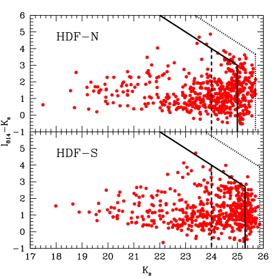
Figure 9: $I_{814}-K_{s}$ CM diagrams for the $K_{s}$-band selected subsamples. Thick solid lines illustrate the limiting colours computed according to Table 1, corresponding to $80$% of the cumulative histogram of apparent magnitudes, whereas thick dotted lines correspond to the very faint limit of magnitudes in the whole catalogue. The dashed lines represent the actual limits used to compute the LFs.

Obviously, also photometric surveys are affected by incompleteness. The SUNY catalogue in the HDF-N is, by construction, an $I_{814}$ band selected sample (Fernandez-Soto et al. fsoto (1999)), whereas objects in the ISAAC HDF-S catalog are detected on the $V_{606}+I_{814}$ image. Even though we use a $K_{s}$ limited sample in the subsequent calculations, it is worth to check on the possible color-selection effects which could affect the two fields in different ways. Figures 3 and 9 display the color-redshift and color-magnitude diagrams. As shown in Fig. 9, very red objects in $I_{814}-K_{s}$, with faint $K_{s}\geq 24.5$ magnitudes, could be missed due to selection criteria. To avoid such effects of colour selection, we adopted a limiting magnitude $K_{s}=24$, corresponding to S/N $\sim$ 3. Moreover, this selection allows us to use the whole area of $5.31$ arcmin² in the HDF-N, combination of the Z1 and Z2 zones, because at this limit the colour distributions of objects with redshifts between $0$ and $2$ have a similar average: $\left<I_{814}-K_{s}\right>=1.28$ in Z1 and $0.95$ in Z2, with a large dispersion in both zones. In the Z2 zone, even for the faintest objects in $K_{s}$, the colours up to $2$ – $2.5$ are allowed: in the Z1 zone most objects have colours below this value, thus we do not introduce any bias by combining the data belonging to the two zones.

At the selected limit in magnitude, blue galaxies have about the same chance to be observed than the reddest ones in the $K_{s}$-band selected subsamples in both fields.

Another type of incompleteness could arise from the surface brightness effect: when objects are detected at bright surface brightness limit, then the LF estimate could be affected, with $M^{*}$ becoming fainter, $\phi^{*}$ smaller and $\alpha$ slightly flatter (Cross & Driver cross (2002) and references therein). In our case, the detection up to faint surface brightness used by the authors of the catalogues ($\mu_{\rm lim}(I_{8}14)\simeq 26$ arcsec^-2 in both the HDF-N and HDF-S) will not induce significant effects on the LF estimates. In particular, the bright end of the LF, on which we base our conclusions, will not suffer strongly from the mentioned effect. The same inference can be demonstrated for other types of incompleteness, such as the detection and measurement algorithm, or the cosmological dimming of surface brightness, discussed by Yoshii (yoshii (1993)) and Totani & Yoshii (totani (2000)), affecting the very faint part of the sample at the limit of the selection and then unable to invalidate our conclusions.

The quantity $V_{\rm max}$ used in the $1/V_{\rm max}$ method to compute LFs can also be used to test the completeness of the sample: if the set of observed galaxies is complete, we expect that they populate uniformly the volume of the survey, i.e. that the galaxies are randomly distributed inside their $V_{\rm max}$ volume. This corresponds to the condition $\left<V/V_{\rm max}\right>=0.5$, where $V$ is the volume characteristic of each galaxy, given its redshift and the limiting magnitude of the survey. However, this line of reasoning is valid only if the population does not evolve in luminosity and it is spatially homogeneous. Larger or smaller values can have different origins. When the sample is subject to magnitude incompleteness to the limiting magnitude (the more distant galaxies become undetectable), the volume $V_{\rm max}$ becomes too big and we have $\left<V/V_{\rm max}\right><0.5$. The same effect can be the result of luminosity evolution, if the nearest objects are also the intrinsically brightest ones. A value $\left<V/V_{\rm max}\right>>0.5$ could be the effect of luminosity evolution, with the brightest objects being the most distant ones. In Sect. 5 we list the values of $\left<V/V_{\rm max}\right>$ averaged over $100$ Monte Carlo realizations, which actually range between $0.43$ and $0.54$, thus very close to the theoretical completeness value.

4.5 Test of the method through mock catalogues

The reliability of the method has been tested by means of mock catalogues. To this aim, we used template galaxies belonging to four spectral types, built from the GISSEL98 library (Bruzual & Charlot bruzual (1993)), corresponding to a star formation in a single burst, star formations with timescales $\tau=3$ Gyr and $\tau=15$ Gyr, and a continuous star formation, each one with Scalo (scalo (1986)) IMF. The four spectral types match the coulours of Elliptical, Sa, Sc and Irregular galaxies. A single, nonevolving luminosity function is used, with a fraction of $\phi^{*}$ assigned to each type following the mix of morphological types in the local universe used by Pozzetti et al. (pozz (1996)) to build their PLE models. In particular, we assigned a fraction of $0.28$, $0.47$, $0.22$ and $0.03$ to the four types, from early to late, assuming that these fractions remain valid beyond the original limit of $b_{J}\leq 16.5$.

Figure 10: The input and recovered LFs for $3$ mock catalogues in two redshift ranges, selecting objects with $K\leq 24$, i.e. $S/N\geq 3$. Triangles and circles represent the binned LFs recovered with the $1/V_{\rm max}$ and the $C^{-}$ methods respectively. The points relative to the $1/V_{\rm max}$ method have been shifted by $-0.15$ magnitudes to avoid superpositions. Error bars represent $10$ and $90$% of the distribution of values obtained with the Monte Carlo method. The solid line is the Schechter function recovered using the STY method, and the dotted lines are the $10$ and $90$% STY functions. The thick dashed line is the input LF.

The number of galaxies in a redshift slice $[z,z+\Delta z]$ and in a range of absolute magnitude $[M,M+\Delta M]$ has been computed by the following integrals:

$$N(z,z+\Delta z;M,M+\Delta M)=$$ (9)

$$\qquad\qquad\omega\int_{z}^{z+\Delta z}\int_{M}^{M+\Delta M}\phi_{\rm input}(M)\,dM\frac{dV}{dz}\,dz\>,$$

where $\omega$ is the solid angle covered by the survey, $\phi_{\rm input}(M)$ is the input Luminosity Function and $dV$ is the volume, dependent on the cosmology. Apparent magnitudes in all the filters are computed from the absolute magnitude $M$, the template spectra and the redshift $z$. We decided to compute apparent magnitudes using the inversion of equation 8, viz applying only the $k$-correction on the evolved SED, because here we are interested only in testing the reliability of the output compared with the input data, using the same procedure adopted for real data. In a realistic case the evolutionary correction becomes important: recovering absolute magnitudes with equation 8 should produce an evolution of the measured LF even if the input LF is nonevolving, as discussed in Sect. 4.3.

For the input LF we imposed a Schechter functional form in the $K$ band, with parameters $\alpha=-1.40$, $M^{*}_{K}=-23.14$ in AB magnitudes and a normalization $\phi^{*}=0.002\,{\rm Mpc}^{-3}$, setting $H_{0}=50\,{\rm km\,s^{-1}\,Mpc^{-1}}$. We used the same cosmology to build mock catalogues and to recover the LF. We discuss the influence of the world models in this kind of calculation in Sect. 5.3.

In our simulated catalogues, we reproduce the same observational effects affecting the real catalogues of the HDFs. In particular, the signal-to-noise ratio behaviour in each filter band is set to be consistent with the data. Galaxies included in the mock catalogues have magnitudes brighter than the limiting magnitude, otherwise their magnitude is set equal to $99$, corresponding to a non detected object in the syntax of hyperz. The limiting magnitude corresponds to a signal-to-noise ratio $S/N=1$, for consistency with the real HDFs catalogues, but we considered only objects with $S/N\geq 3$ to estimate LFs. The photometric error is computed as a function of magnitude for each filter, after specifying a signal-to-noise ratio reached at a given magnitude, matching the same ratios computed for the HDFs catalogues and using a similar procedure as in Bolzonella et al. (hyperz (2000)). A random reddening with $A_{V}$ ranging from $0$ to $1$ is also applied to SEDs. To allow a photometric redshift estimate, we included in the catalogues only objects detected in at least $3$ filters. The number of galaxies included in a mock catalogue has been computed using a surface similar to the HDFs, i.e. $5$ arcmin². In this way we obtained $N_{\rm obj}$ objects, to which we added a fluctuation due to Poissonian statistics, $\pm{\rm random}[0,\sqrt{N_{\rm obj}}]$. Objects have been randomly selected from a larger field, to allow the selection of bright objects at low redshift. The final catalogues have roughly the same number of objects as the HDFs, with the same observational characteristics.

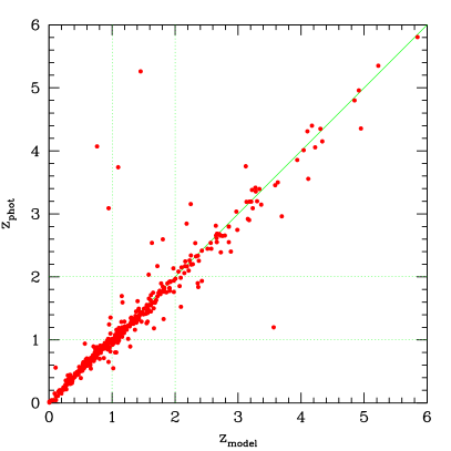
Figure 11: Comparison between the input redshift $z_{\rm model}$ and the photometric redshift best fit $z_{\rm phot}$ for the objects with $K\leq 24$

in the simulated catalogue used to recover the input LF in the upper panel of Figure 10. Dotted lines identify the two considered redshift bins.

Next, we computed photometric redshifts for these simulated galaxies, using all the available SEDs, and we used the hyperz outputs (the probability function of redshift, the SED parameters) to estimate absolute magnitudes and then the Luminosity Functions by means of the Monte Carlo method described in the previous section, selecting objects in the $K_{s}$ and with magnitudes $K_{s}\leq 24$, i.e. $S/N\geq 3$.

The recovered LFs for $3$ random catalogues are shown in Fig. 10 for two redshift ranges. The mean parameters obtained averaging over a set of $10$ random catalogues are $\overline{\phi^{*}}=0.00267\pm 0.00141\,{\rm Mpc}^{-3}$, $\overline{M^{*}_{K}}=-22.958\pm 0.771$ and $\overline{\alpha}=-1.441\pm 0.083$ in the redshift range $z=0$ – $1$. The estimated errors in these values correspond to the standard deviation ($1\sigma$) of the distribution of values used to compute the arithmetic mean and do not take into account the errors inferred from each Monte Carlo realization. The agreement of these values with the input ones is remarkable. In the redshift range $z=1$ – $2$ the recovered parameters are $\overline{\phi^{*}}=0.00259\pm 0.00207\,{\rm Mpc}^{-3}$, $\overline{M^{*}_{K}}=-22.611\pm 0.489$, $\overline{\alpha}=-1.681\pm 0.208$. In this case the normalization is well recovered, even if the large error reflects the large scatter in the values obtained in different realizations; the value of $M^{*}_{K}$ is consistent with the input one, whereas the recovered $\alpha$ is slightly overestimated even considering the $1\sigma$ error.

The comparison between the input value of the redshift and the photometric redshift best fit is shown in Fig. 11 for the objects with $S/N\geq 3$ in $K$ magnitudes: for these objects the photometric redshift is a very good estimate of the input one and we do not see the degeneracy between different redshift ranges, characteristic of the faintest objects with lower signal-to-noise ratio (see Bolzonella et al. hyperz (2000)). Only few objects are erroneously attributed to high redshifts: these objects are very faint galaxies, non detected in the $U_{300}$ and $V_{450}$ filters, determining a confusion in the location of the Lyman break.

In Fig. 12 the input absolute magnitude is compared to the absolute magnitude computed by hyperz, using the redshift and the spectral type best fit. The objects represented in these two panels have been selected using their photometric and their input redshifts, in the two redshift bins shown in Fig. 10. We considered only objects with $K\leq 24$, i.e. the same objects used in the LF estimate. The agreement is very good, with very few outliers. In the left panel, we can notice the rapid decrease of galaxies with $M_{K}\ga-16$, producing large error bars in the binned estimate of the LF. In the range between $z=1$ and $2$, the lack of faint objects due to observational limits prevents a good estimate of the faint-end slope $\alpha$ using the STY method. Nevertheless, the bright end is well reproduced by the binned methods.

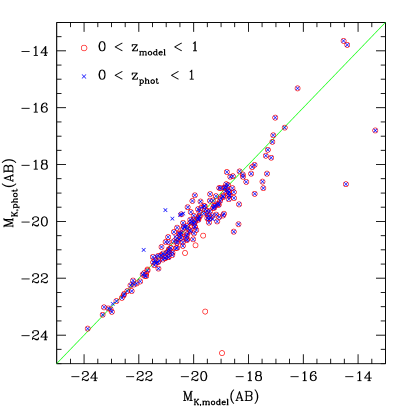
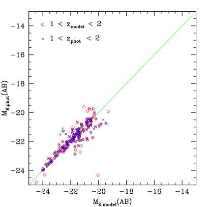
Figure 12: Comparison between the input absolute magnitude $M_{K,{\rm model}}$ and the absolute magnitude computed using the photometric redshift best fit $M_{K,{\rm phot}}$, for the mock catalogue used in the upper panel of Fig. 10 and objects with $K\leq 24$. Left: redshift range $z=0$ – $1$. Right: $z=1$ – $2$. Circles and crosses represent the points selected following the input redshift and the photometric redshift respectively.

Similar analysis comparing methods for LF estimate through simulations have been carried out by other authors. Willmer (willmer (1997)) found that the STY method tends to slightly underestimate the faint-end compared to the input value. In our case, we found a small overestimate of $\alpha$, but the large error bars are consistent with the input value. Concerning the non parametric methods, the study of Takeuchi et al. (take (2000)) demonstrated that for large and spatially homogeneous samples the LF estimate is not biased, whereas the faint-end is subject to large fluctuations when the sample is small. The overestimate of the low redshift LF on the faintest bins is similar to ours, according to their figures, and still consistent with the input LF due to the large error bars. On the contrary, at higher redshift we see a decline in the faintest bins, that is also been shown by Liu et al. (liu (1998)).

In summary, the procedure used to recover the LF in the range $z=0$ – $1$ can be considered as reliable, and we did not try to take into account the small systematic effects mentioned above. In the range $z=1$ – $2$, the results of the STY method have to be taken with care, but the non parametric estimate of the LF still provides a good fit of the bright-end.

5 Near infrared luminosity functions in the HDFs

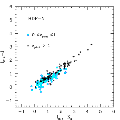
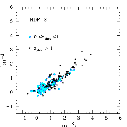
Figure 13: NIR colour-colour plot: $I_{814}-K_{s}$ vs $I_{814}-J$ for the HDF-N and HDF-S. Limiting magnitudes are $I_{814}=28.5$, $J=24.6$ and $K_{s}=24.0$, corresponding to $S/N=3$.

We compute the LFs using the three methods described in Sect. 4.1. In particular, for the non-parametric methods we adopt a binning of $1$ magnitude or $2$ magnitudes at the faint end to have a conspicuous number of objects in each bin. To compute the luminosity functions we divide the sample in redshift slices, larger than the typical errors of photometric redshifts, to minimize the change of redshift bin and to study the redshift evolution of the LFs. The adopted limiting magnitude is $K_{s}=24$ in both the HDF-N and HDF-S. Following the procedure described above, we iterate the computation of the binned or parametrized LF. We choose to realize $100$ iterations, sufficient to estimate the effect of random selection of redshifts. During the photometric redshift calculation we impose a range of absolute $B$ magnitudes: solutions with $M_{B}$ outside the range $[-28,-9]$ are considered forbidden also when estimating the LF.

Because the $K_{s}$-band is the reddest one, the absolute magnitudes have been computed using always the $K_{s}$ apparent magnitudes. Studying the $K$-band at redshifts $z\sim 2$ means to map the rest-frame $I$-band emission: in Fig. 13 we show that these magnitudes are strictly correlated and thus they basically map the same stellar population. This behaviour can be explained considering the emitting stellar population: even at $z\sim 2$ the luminosity at the wavelengths covered by the $K_{s}$ filter is always produced by the old star population, the $4000$ Å break still being inside the $J$ filter. Furthermore, $K_{s}$ magnitudes are not affected by recent bursts of star formation. For this reason, and because of the characteristics of the $k$-correction discussed in Sect. 4.3, we considered that we can safely compute $K_{s}$-band absolute magnitudes at least up to a redshift of $2$.

We have also estimated the $J$-band LF in the redshift range $z=[0,1]$ from the $J$-selected subsample, and in the redshift range $[1,2]$ by selecting the objects in the $K_{s}$-band sample that better approximate the $J$ filter rest frame.

We will study the LF in the optical bands and in the UV in a forthcoming paper (Bolzonella et al. in preparation).

5.1 $K_{s}$-band LF

Up to now, the $K_{s}$-band LF has been estimated only for data in redshift surveys, and for this reason the accessible range of redshifts to be explored was limited. In Table 2 we report previous estimates, mainly retrieved from the table by Loveday (loveday (2000)), completed with a guess of the magnitude and redshift ranges of the samples. Magnitudes have been transformed into the AB system by means of the conversion provided in Table 1 and the dependence from the Hubble constant has been explicited using the Hubble parameter $h=H_{0}/(100\,{\rm km\,s^{-1}\,Mpc^{-1}})$.

Table 2: Compilation of other $K_{s}$-band LFs for field galaxies in redshift surveys, in general obtained with cosmological parameters $\Omega_{0}=1$; the data are transformed into AB magnitudes in the filter $K$. Errors are in general given at $1\sigma$ of confidence likelihood contours. Modified and updated from Loveday’s (loveday (2000)) table.

Author(s)	$\phi^{*}$ [$h^{3}\,$Mpc-3]		$M^{*}_{K}-5\log h$		$\alpha$		$M_{K}-5\log h$ range	$z$ range	other remarks
Mobasher et al. (mobasher (1993))	$0.0112$$\pm$	$0.0016$	$-21.51$$\pm$	$0.3^{1}$	$-1.0$$\pm$	$0.3$	$[-23.5,-19.0]$	$0.0\leq z\la 0.1$	AARS
Glazebrook et al. (glaze (1995))	$0.029$$\pm$	$0.007$	$-21.15$$\pm$	$0.23^{2}$	$-1.04$$\pm$	$0.31$	$[-22.5,-18.5]$	$0.0<z<0.2$
Glazebrook et al. (glaze (1995))	$0.019$$\pm$	$0.002$	$-21.44$$\pm$	$0.11^{2}$	$-1.04$$\pm$	$0.31$	$[-24.0,-18.5]$	$0.0<z<0.8$
Cowie et al. (cowie2 (1996))	$0.016$		$-21.63$		$-1.25$		$[-23.5,-16.5]$	$0.0<z\la 1.6$	$K$-band selected
Gardner et al. (gardner (1997))3	$0.0182$		$-21.50$$\pm$	$0.17$	$-1.03$$\pm$	$0.24$	$[-23.5,-18.0]$	$\left<z\right>=0.14$	$K$-band selected
Szokoly et al. (szokoly (1998))	$0.012$$\pm$	$0.004$	$-21.72$$\pm$	$0.3$	$-1.27$$\pm$	$0.2$	$[-23.5,-18.5]$	$0.0<z\la 0.5$	$K$-band selected
Loveday (loveday (2000))	$0.012$$\pm$	$0.008$	$-21.71$$\pm$	$0.42$	$-1.16$$\pm$	$0.19$	$[-24.0,-14.0]$	$\left<z\right>=0.05$	Stromlo-APM
Kochanek et al. (kocha (2001))4	$0.0116$$\pm$	$0.001$	$-21.52$$\pm$	$0.05$	$-1.09$$\pm$	$0.06$	$[-24.0,-18.5]$	$0.01\la z\la 0.05$	2MASS
Cole et al. (cole1 (2001))	$0.0108$$\pm$	$0.0016$	$-21.57$$\pm$	$0.03$	$-0.96$$\pm$	$0.05$	$[-24.0,-17.0]$	$0<z\la 0.2$	2dF - $\Lambda$CDM
Balogh et al. (balogh (2001))5	—		$-21.61$$\pm$	$0.08$	$-1.10$$\pm$	$0.14$	$[-24.0,-18.0]$	$0<z\la 0.18$

¹ From Loveday (loveday (2000)): added $0.22$ magnitudes due to different method for $k$-corrections.
² From Loveday (loveday (2000)): aperture correction of $-0.30$ magnitudes.
³ The value adopted is relative to the $q_{0}=0.5$ model with only $k$-correction.
⁴ Isophotal magnitude selection $7<K_{20}<11.25$.
⁵ Normalized to the weighted number of galaxies brighter than $K_{\rm Vega}=-21.5$.

Using the HDF-N and HDF-S catalogues we can reach unprecedented depths: we estimated for the first time the LFs in the $K_{s}$ band for objects with $z_{\rm phot}\in[0,1]$ and $[1,2]$.

We selected the subsamples in each redshift range after the randomization procedure of redshifts. The values of $\left<V/V_{\rm max}\right>$ averaged over the Monte Carlo realizations are $0.54,0.44$ in the redshift ranges $z_{\rm phot}\in[0,1],[1,2]$ for the HDF-N and $0.51,0.47$ for the HDF-S in the same redshift ranges.

Figure 14 illustrates our estimate of the $K_{s}$ band LFs for the HDF-N and the HDF-S. There is a good agreement between the local $K$-band LF computed by Cowie et al. (cowie (1994, 1996)) and the $z_{\rm phot}\in[0,1]$ sample, especially in the HDF-S. In the case of the $z_{\rm phot}\in[1,2]$ sample, our results are still compatible with the local values. A slight negative evolution is observed between the $[0,1]$ and $[1,2]$ bins when comparing the non-parametric estimates for galaxies fainter than $M_{K}=-21$. This trend is hardly significant. The fact that the $1/V_{\rm max}$ and $C^{-}$ estimates are very close means that there are no artifacts due to clustering.

Table 3: Parameters of the $K_{s}$-band LF for galaxies in the HDF-N and HDF-S obtained with the STY method.

$z$ range	Cosmology	Field	$\phi^{*}$ [$h^{3}\,$Mpc-3]	$M^{*}_{K}({\rm AB})-5\log h$	$\alpha$	$M_{K}-5\log h$ range
$0\leq z<1$	$\Omega_{0}=1$, $\Omega_{\Lambda}=0$	HDF-N	$0.0342^{+0.0065}_{-0.0084}$	$-21.540^{+0.164}_{-0.247}$	$-1.101^{+0.066}_{-0.070}$	$[-23.0,-12.0]$
		HDF-S	$0.0232^{+0.0087}_{-0.0073}$	$-21.860^{+0.286}_{-0.279}$	$-1.159^{+0.093}_{-0.084}$	$[-23.0,-12.0]$
	$\Omega_{0}=0.3$, $\Omega_{\Lambda}=0.7$	HDF-N	$0.0121^{+0.0029}_{-0.0036}$	$-22.266^{+0.238}_{-0.501}$	$-1.164^{+0.064}_{-0.076}$	$[-24.0,-12.0]$
		HDF-S	$0.0100^{+0.0039}_{-0.0031}$	$-22.389^{+0.257}_{-0.297}$	$-1.170^{+0.089}_{-0.095}$	$[-23.0,-12.0]$
$1\leq z<2$	$\Omega_{0}=1$, $\Omega_{\Lambda}=0$	HDF-N	$0.0050^{+0.0029}_{-0.0017}$	$-22.524^{+0.373}_{-0.382}$	$-1.579^{+0.098}_{-0.079}$	$[-23.5,-17.0]$
		HDF-S	$0.0083^{+0.0074}_{-0.0059}$	$-22.201^{+0.624}_{-1.64}$	$-1.411^{+0.080}_{-0.159}$	$[-22.5,-17.5]$
	$\Omega_{0}=0.3$, $\Omega_{\Lambda}=0.7$	HDF-N	$0.0017^{+0.0008}_{-0.0005}$	$-23.200^{+0.259}_{-0.379}$	$-1.568^{+0.099}_{-0.088}$	$[-24.0,-17.5]$
		HDF-S	$0.0024^{+0.0025}_{-0.0017}$	$-23.065^{+0.738}_{-1.541}$	$-1.424^{+0.222}_{-0.174}$	$[-23.0,-18.0]$

Figure 14: $K_{s}$-band LFs for galaxies in the HDF-N and HDF-S in two redshift bins, assuming a limiting magnitude $K_{s}=24.0$ and a cosmological model with $\Omega_{0}=1$. Triangles and circles represent the median of the results obtained with the $1/V_{\rm max}$ and the $C^{-}$ methods respectively. The upper panels represent the LF for galaxies with $z_{\rm phot}$ in $[0,1]$, the lower in $[1,2]$. The points relative to the $1/V_{\rm max}$ method have been shifted of $-0.15$ magnitudes for clarity. The error bars corresponding to $10$ and $90$ percentiles of the distribution are also shown. The solid line shows the LF obtained with the STY method. The LF obtained by Cowie et al. (cowie2 (1996)) (dashed line) is shown as reference LF. In the lower panels, the $z_{\rm phot}=[0,1]$ LF (thin solid line) is also displayed for comparison.

In Table 3 we list the parameters of the STY estimate for the $[0,1]$ and $[1,2]$ samples. The most impressive results we can note from Fig. 14 are the very wide range of absolute magnitudes covered by the data and the possibility of computing for the first time the NIR LFs at redshifts in the range $[1,2]$, where many difficulties arise for the traditional spectroscopy. Moreover, this redshift range is of paramount importance in the study of galaxy formation and evolution, as we will discuss in Sect. 6.

Figure 15: Parameters of the LFs as a function of the redshift bin for the two cosmologies adopted in the paper. Results obtained with the $\Omega_{0}=1$ and $\Omega_{0}=0.3,\Omega_{\Lambda}=0.7$ cosmologies have been shifted in redshift by $-0.05$ and $+0.05$ respectively.

In Fig. 15 we summarize the results given in Table 3, showing the $\alpha$ and $M^{*}_{K}({\rm AB})$ parameters and their respective errors as a function of redshift, derived for the two adopted cosmologies.

5.2 $J$-band LF

We also computed LFs in the $J$-band. In this case, we selected galaxies in the $J$ filter when considering the lowest redshift bin [0,1], whereas we estimated the $J$-band in the highest redshift range ($z_{\rm phot}\in[1,2]$) using the $K_{s}$-band selected subsamples. In this way we select the objects approximately in the $J$-band rest-frame and we can check if the assumptions made for the $K_{s}$ band LF computation were safe. We selected objects in the HDF-N with $J\leq 24.6$ in the redshift range $[0,1]$ and with $K_{s}\leq 24$ in $z=[1,2]$, corresponding to objects with $S/N\geq 3$. At these limits the colours in the HDF-N and HDF-S are very similar: at $J=24.6$, the mean $I_{814}-J$ in $[0,1]$ is $0.57$ in the HDF-N and $0.50$ in the HDF-S; at $K_{s}=24$ the mean $I_{814}-K$ in $z=[1,2]$ is $1.65$ in the HDF-N and it is $1.85$ in the HDF-S.

The values of $\left<V/V_{\rm max}\right>$ are $0.56,0.43$ in the redshift ranges $z_{\rm phot}\in[0,1]$ and $[1,2]$, respectively, for the HDF-N, and $0.51,0.47$ in the same redshift ranges for the HDF-S.

Figure 16: $J$-band LFs for galaxies in the HDF-N and HDF-S in two redshift bins, assuming a limiting magnitude $J=24.6$ in the redshift range $[0,1]$ and $K_{s}=24.0$ in $z=[1,2]$, and a cosmological model with $\Omega_{0}=1$. Same symbols as in Fig. 14. The LF obtained by Cole et al. (cole1 (2001)) (dashed line) assuming the same cosmological model is also shown as reference LF. In the lower panels, the LF in the $z_{\rm phot}=[0,1]$ interval is also displayed for comparison (thin solid line).

Table 4: Parameters of the $J$-band LF for galaxies in the HDF-N and HDF-S obtained with the STY method.

$z$ range	Cosmology	Field	$\phi^{*}$ [$h^{3}\,$Mpc-3]	$M^{*}_{J}({\rm AB})-5\log h$	$\alpha$	$M_{J}-5\log h$ range
$0\leq z<1$	$\Omega_{0}=1$, $\Omega_{\Lambda}=0$	HDF-N	$0.0357^{+0.0064}_{-0.0064}$	$-21.537^{+0.225}_{-0.264}$	$-1.106^{+0.091}_{-0.055}$	$[-23.0,-11.0]$
		HDF-S	$0.0281^{+0.0086}_{-0.0049}$	$-21.942^{+0.280}_{-0.253}$	$-1.090^{+0.089}_{-0.046}$	$[-23.0,-11.0]$
	$\Omega_{0}=0.3$, $\Omega_{\Lambda}=0.7$	HDF-N	$0.0158^{+0.0022}_{-0.0027}$	$-22.077^{+0.185}_{-0.333}$	$-1.066^{+0.036}_{-0.044}$	$[-24.0,-11.5]$
		HDF-S	$0.0129^{+0.0033}_{-0.0025}$	$-22.451^{+0.244}_{-0.230}$	$-1.082^{+0.075}_{-0.047}$	$[-23.5,-11.5]$
$1\leq z<2$	$\Omega_{0}=1$, $\Omega_{\Lambda}=0$	HDF-N	$0.0189^{+0.0076}_{-0.0108}$	$-21.788^{+0.380}_{-1.423}$	$-1.080^{+0.193}_{-0.175}$	$[-23.5,-17.0]$
		HDF-S	$0.0251^{+0.0084}_{-0.0126}$	$-21.439^{+0.400}_{-1.053}$	$-0.773^{+0.199}_{-0.301}$	$[-22.0,-17.0]$
	$\Omega_{0}=0.3$, $\Omega_{\Lambda}=0.7$	HDF-N	$0.0061^{+0.0028}_{-0.0036}$	$-22.431^{+0.376}_{-1.652}$	$-1.047^{+0.175}_{-0.195}$	$[-24.0,-17.5]$
		HDF-S	$0.0074^{+0.0026}_{-0.0040}$	$-22.357^{+0.605}_{-1.273}$	$-0.796^{+0.229}_{-0.317}$	$[-23.0,-17.5]$

In Fig. 16 we plot the LFs obtained with the adopted parametric and non parametric methods in the redshift ranges $[0,1]$ and $[1,2]$, as well as the Cole et al. (cole1 (2001)) local LF estimated in the 2dFGRS, shown as a reference. Our estimate and the Cole et al. (cole1 (2001)) one, suitably transformed in AB magnitudes ($M^{*}_{J}=-21.40$, $\alpha=-0.93$, $\phi^{*}=0.0108$ computed with cosmology $\Omega_{0}=1,\Omega_{\Lambda}=0$ and only $k$-correction to match the same conditions we used), seem to be in disagreement, mainly in the normalization. However, the comparison between our LF estimate obtained in the flat $\Lambda$-dominated cosmology and the analogous one computed by Cole et al. cole1 (2001) partially mitigates the difference.

Table 4 contains the values of the Schechter parameters of the $J$-band LF obtained in the two redshift ranges for the HDF-N and HDF-S. We have also computed the LF in the $H$ and $I$ bands for the HDF-N and HDF-S catalogues. In all cases, we found similar results for the two fields.

5.3 Effect of cosmology

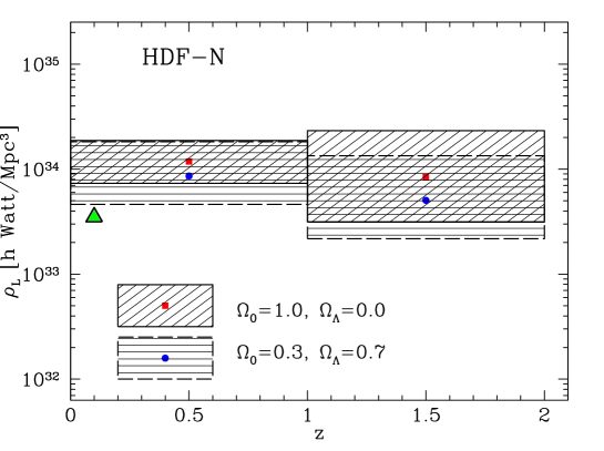
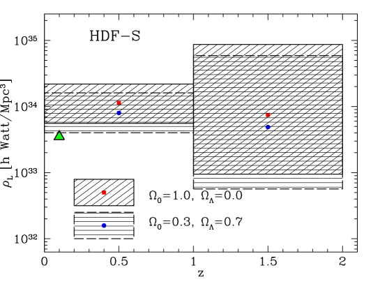
Figure 17: The luminosity density in the $K_{s}$-band, as obtained from the values listed in Table 3. Squares: luminosity densities computed using the median values of the STY estimate of the LF in the case of a $\Omega_{0}=1$ cosmological model. Circles: values of the luminosity density in a flat cosmological constant dominated universe. The value obtained by Cole et al. (cole1 (2001)) is also shown for comparison as a triangle.

We estimated LFs in two cosmologies: the “old” Standard CDM with $\Omega_{0}=1$ and $\Omega_{\Lambda}=0$, and a flat cosmological constant dominated model, that nowadays is the most accepted one, with $\Omega_{0}=0.3$ and $\Omega_{\Lambda}=0.7$. The influence of cosmology in the photometric redshift computation is negligible, as discussed by Bolzonella et al. (hyperz (2000)), thus we used the same photometric redshifts to estimate the LFs in different cosmologies.

When LFs are computed at low redshifts, we expect little or no differences in the estimates, as in the case of the 2dFGRS by Cole et al. (cole1 (2001)), where the difference in the value of $M^{*}_{K_{s}}$ between the two interesting models is $0.16$ magnitudes. Therefore, whereas local estimates are not affected by the change of cosmology, when we are dealing in particular with galaxies at high redshifts the variation of volume and distances become substantial. As expected, looking at Tables 3 and 4 we can remark that the value of $M^{*}$ brightens when the lambda dominated cosmology is assumed, whereas $\phi^{*}$ decreases because of the increase of the comoving volume at a given redshift. In fact, the difference in distance modulus will affect absolute magnitudes, whereas the difference in volumes affects the estimate of the $\phi^{*}$ parameter.

5.4 NIR Luminosity Density

Using the values of the Schechter parameters listed in Tables 3 and 4 we computed the luminosity density, given by

$$\rho_{L}=\int L\phi(L)\,dL=\phi^{*}L^{*}\Gamma(\alpha+2)\>.$$ (10)

Results are shown in Fig. 17, in units of $h\,{\rm W\,Mpc^{-3}}$, derived from the usual solar luminosity values, after integration and scaling through a stellar solar type SED (taken from the library of Pickles pickles (1998)). Boxes represent the maximum and minimum values obtained using the Schechter parameters in a given redshift range. We show the results for both the adopted cosmological models: we can see that the luminosity density does not strongly depend on cosmology, being the values relative to one model inside the boxes of the second one. The most remarkable characteristic visible in Fig. 17 is that the luminosity density is consistent with non-evolution at least up to a redshift $z\sim 2$.

As expected from the comparison of our Schechter parameters with the values in Table 2, our estimates of $\rho_{K_{s}}$ are higher than the luminosity densities computed for instance by Cole et al. (cole1 (2001)) for the 2dFGRS: their value in the $K_{s}$-band, conveniently converted into $h\,{\rm W\,Mpc^{-3}}$ in the $K_{s}$ filter, is $\rho_{K_{s}}=3.5\times 10^{33}\,h\,{\rm W\,Mpc^{-3}}$. It is shown as a triangle in Fig. 17: it is marginally consistent with our lower limit of the $z\in[0,1]$ estimate in the HDF-N and HDF-S for the $\Lambda$-dominated model (the same model adopted by Cole et al. cole1 (2001)). In the $J$-band, our estimates in the redshift range $[0,1]$ are $\rho_{J}=3.53\times 10^{34}(3.86\times 10^{34})$ and $2.35\times 10^{34}(2.49\times 10^{34})\,h\,{\rm W\,Mpc^{-3}}$ in the HDF-N (HDF-S), for the matter and $\Lambda$-dominated models respectively, whereas the value found by Cole et al. (cole1 (2001)) is $6.8\times 10^{33}\,h\,{\rm W\,Mpc^{-3}}$.

In a recent paper, Wright (wright (2001)) already claimed that the value obtained by Cole et al. (cole1 (2001)) does not match the extrapolation to the NIR from the optical luminosity densities obtained in the SDSS by Blanton et al. (blanton (2001)). The discrepancy is about a factor of $2.3$. On the contrary, the present results are in much better agreement with the SDSS optical luminosity densities. This result has to be considered with caution because of the small size of the HDFs.

5.5 Mass Function

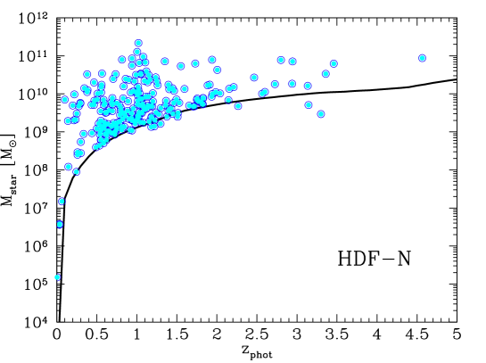
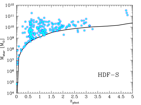
Figure 18: The masses of the objects in the $K_{s}$-band selected subsamples with $K_{s}\leq 24.0$ in the HDF-N and HDF-S, computed assuming a mass-to-light ration of $0.8$ in solar units. The solid line represents the limiting mass inferred from the limiting magnitude $K_{s}=24.0$.

The $K$-band luminosity is considered as a good tracer of the stellar mass in galaxies, because the bulk of the emission at these wavelengths is dominated by solar stars, that constitute most of the mass in stars. Moreover, the $K$-band estimator is nearly independent on the star formation history and then it can be safely used to compute the baryonic mass contained in galaxies.

We adopted a constant stellar mass-to-light ratio: $M_{\rm star}/L_{K}=0.8\,M_{\odot}/L_{K\odot}$, a mean value obtained from the estimate by Worthey (worthey (1994)) considering the range of ages spanned by our objects. In any case the dependence of $M/L$ with age is not strong in this filter. With this assumption, the LF reflects the stellar mass function: a non evolution in luminosities implies a non evolution in characteristic masses. In Fig. 18 we show the masses computed from the $K_{s}$-band apparent magnitudes of the $K_{s}$-band selected subsample used in this study. We also show the limiting mass as a function of redshift computed for an elliptical galaxy, assuming $K_{s}$-band limiting magnitudes of $24.0$ at which reach $S/N=3$. The change using different SEDs is negligible. According to this figure, the HDFs allow to detect stellar haloes of $\sim 10^{9}M_{\odot}$ up to $z\sim 1$, and around $10^{10}M_{\odot}$ up to $z\ga 3$.

6 Discussion: Galaxy formation models

LFs are a convenient way to describe the galaxy population and to get hints about the mechanisms of formation and evolution of galaxies.

Two scenarios are in competition to explain the history of galaxies up to the present epoch. The formation of elliptical galaxies is especially intriguing, because despite their old and apparently simple stellar population, their process of formation is far from being understood. The two models in competition are:

• The hierarchical scenario, which is based on CDM cosmological models (e.g. Kauffmann et al. kauff1 (1994); Cole et al. cole (2000)). It assumes that galaxies have formed through merging of sub-galactic structures. In particular, elliptical galaxies are born from the merging of two disks of comparable dimensions; during the interaction, a burst of star formation occurs, consuming the gas present in the progenitors, and then passive evolution follows.

• The monolithic scenario, revisited in different ways by many authors, which basically assumes that galaxies formed approximately at the same epoch, with particular details depending on the morphological types (e.g. Rocca-Volmerange & Guiderdoni rocca (1991); Pozzetti et al. pozz (1996)). Ellipticals are believed to form at $z_{\rm form}\ga 2-3$ and, at the time of their assembly, a burst of star formation occurred, followed by passive evolution of the stellar population.

The two scenarios foresee different characteristics as a function of redshift for the progenitors of the blue and red galaxies in the local universe. Moreover, since most of the merging would take place at $z<2$, the redshift range between $1$ and $2$ is fundamental to discriminate between monolithic and hierarchical scenarios. Both mechanisms account for the properties of elliptical galaxies up to $z\simeq 1$, e.g. the CM relation (Gladders et al. glad (1998); Kauffmann & Charlot 1998b ), but, between $z=1$ and $z=2$, the expectations for the photometric properties of all galaxies differ significantly between the two scenarios.

A powerful test to establish what drives the galaxy evolution, was proposed by Kauffmann & Charlot (kauff (1998)), using the $K$-band luminosity function. The luminosity in the $K$ filter is directly linked to the mass in stars and is barely affected by the presence of dust extinction, thus making the $K$ photometry a privileged tool to study galaxy formation. Moreover, galaxies with the same stellar mass have nearly the same $K$ magnitude, independently on their star formation history. For these reasons the $K$-band LF can probe if galaxies were assembled early, according to the monolithic scenario, or recently from mergers. Kauffmann & Charlot (kauff (1998)) built two PLE models with density parameters $\Omega_{0}=1$ and $\Omega_{0}=0.2$ and two hierarchical models based on the CDM cosmology, with the same values of $\Omega_{0}$. They computed the evolution of the $K$-band LF at increasing redshifts for the PLE models and for the $\Omega_{0}=1$ hierarchical model, each one able to reproduce the local LF. On the contrary, their low density hierarchical model failed to reproduce the local $K$-band LF and they did not compute the evolution of the LF in this framework.

At redshifts $z>1$ a sharp difference between the two models is predicted, as explained in Kauffmann & Charlot. The PLE models foresee a constant bright-end for the LF, with small differences between the flat and the open cosmology, whereas the hierarchical model considered by Kauffmann & Charlot undergoes a shift toward faint magnitudes (see Fig. 19).

The development of hierarchical scenarios in open or flat cosmological models with cosmological constant mitigates the discrepancy between these two scenarios (monolithic vs. hierarchical), because the epoch of the major merging moves at higher redshifts (Fontana et al. fontana (1999), Cole et al. cole (2000)). In this case, the PLE model could not be distinguished from a scenario where the galaxy assembly occurs at early epochs, followed by a passive evolution of the stellar population. Our results for the cumulative redshift distribution actually support such scenarios (see Fig. 6).

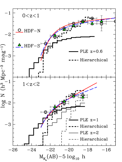
Figure 19: Comparison between the theoretical luminosity functions derived by Kauffmann & Charlot (kauff (1998)) and the present results on the HDFs. Histograms represent the prediction for the hierarchical, $\Omega_{0}=1$ CDM, (dashed line) and PLE scenarios (solid line). The solid and long dashed continuous lines display respectively the STY LFs fitted to the data in the HDF-N and HDF-S. Circles and triangles show the estimate of the LF with the $C^{-}$ method in the HDF-N and HDF-S. In the lower panel we show the model predictions both at $z=1$ and $z=2$, because we estimated the LF using galaxies with redshifts between these two extremes.

The present results, i.e. the lack of significant evolution in the bright part of the LF from the redshift range $[0,1]$ to $[1,2]$, provide a stringent clue, supporting the idea that massive galaxies were already in place at high redshifts, against the old CDM hierarchical model adopted by Kauffmann & Charlot. The comparison between these theoretical predictions and the observations derived in the present paper can be found in Fig. 19. In the lower redshift bin, our estimates of the LFs present a faint-end slope in agreement with the hierarchical model, whereas at bright magnitudes the small differences between the two models do not support any claim. In the redshift bin $z=[1,2]$ we have compared our estimate with both the predictions of the models at redshift $z=1$ and $2$: the model predictions suitable for our sample should lie between the two. It is evident from the lower panel of Fig. 19 that the very bright part of the LFs remains well above the hierarchical model predictions at $z=1$ and $2$, being much closer to the predictions of the monolithic/PLE-like scenario. On the other hand, the faint end slope seems to be in better agreement with the hierarchical model, even in this redshift range.

Other recent studies on the Hubble fields, based on different selection criteria, seem to indicate that the formation of elliptical galaxies should be placed at $z>2$ (Benítez et al. benitez (1999); Broadhurst & Bouwens broad (2000)). In the present paper we do not select galaxies according to morphological types, but the same conclusions apply to the most massive (NIR luminous) galaxies in our sample.

The lack of evolution in the bright end of the LF is in good agreement with the results found from spectroscopic surveys. Glazebrook et al. (glaze (1995)) found no evidence for evolution in the $K$-band LF up to $z\leq 0.5$, and concluded that massive spheroids were in place at $z\geq 1$ and then evolved passively. Songaila et al. (songaila (1994)) found a lack of significant evolution in their $K$-band sample up to a redshift of $\sim 1$. Cowie et al. (cowie2 (1996)) found little evolution in their sample of red (old) objects to $z\sim 1$. The present results extend the previous findings in redshift, up to $z\sim 2$, with the same conclusions with respect to the evolution of the most massive galaxies. The comparison between the present LFs in the near-IR and in the optical-UV bands (Bolzonella et al. in preparation) will provide new insights on the galaxy formation scenario.

7 Summary

The results of this paper can be summarized as follows:

1. The photometric redshift technique is an indispensable tool to study the faint-end and the evolution of LFs, pushing the limiting magnitudes toward fainter limits than the works based on spectroscopic surveys.

2. We have elaborated a method to compute the luminosity function properly taking into account the characteristic of the uncertainties of the photometric redshift technique. This approach can be conveniently applied to compute LFs from the forthcoming wide and deep field photometric surveys. Moreover, this method can be easily extended to other wavelengths crucial for the study of galaxy evolution, as optical LFs and the LF at $1500$ Å (Bolzonella et al. in preparation).

3. We have computed the LF in $K_{s}$ and $J$ bands for the HDF-N and HDF-S catalogues with two non-parametric methods, $1/V_{\rm max}$ and $C^{-}$, and with the maximum likelihood method STY, assuming a Schechter functional shape. We found similar results for the two fields. This seems to indicate that clustering does not considerably affect the estimate of the LFs, even for the $1/V_{\rm max}$ method.

4. The bright-end of the NIR LF remains unchanged within the errors up to at least $z\sim 2$. Also the NIR luminosity density is in good agreement with no-evolution, at least up to a redshift $z\sim 2$. This result is consistent with the bulk of the stellar mass being in place and assembled at such redshift.

5. The analysis of the near-IR LF and the cumulative redshift distributions is a powerful test for galaxy formation models. The evidence of an unevolving bright-end of the $K_{s}$-band LF up to $z\simeq 2$ supports the assembly of massive galaxies before such redshift, a result which is rather close to the old monolithic scenario than to the hierarchical standard CDM cosmological model. Our results are consistent with hierarchical scenarios in open or flat cosmological models with cosmological constant (such as Fontana et al. fontana (1999), Cole et al. cole (2000)).

- (1) Arnouts, S., Cristiani, S., Moscardini, L., Matarrese, S., Lucchin, F., Fontana, A. & Giallongo, E. 1999, MNRAS 310, 540
- (2) Arnouts, S., Moscardini, L., Vanzella, E., Colombi, S., Cristiani, S., Fontana, A., Giallongo, E., Matarrese, S. & Saracco, P. 2002, MNRAS 329, 355
- (3) Balogh, M., Christlein, D., Zabludoff, A. & Zaritsky, D. 2001, ApJ 557, 117
- (4) Benítez, N., Broadhurst, T., Bouwens, R., Silk, J., & Rosati, P. 1999, ApJ 515, L65
- (5) Bertin, E. & Arnouts, S. 1996, A&ASS 117, 393
- (6) Blanton, M. R., Dalcanton, J., Eisenstein, D., Loveday, J., Strauss, M. A., SubbaRao, M., Weinberg, D. H. and the SDSS collaboration, 2001, AJ 121 2358
- (7) Bower, R. G., Lucey, J. R. & Ellis, R. S. 1992, MNRAS 254, 601
- (8) Bower, R. G., Kodama, T. & Terlevich, A. 1998, MNRAS 299, 1193
- (9) Bolzonella, M., Miralles, J.-M. & Pelló, R. 2000, A&A 363, 476
- (10) Broadhurst, T., Bouwens, R. J. 2000, ApJ 530, L53
- (11) Bruzual, G. & Charlot, S. 1993, ApJ 405, 538
- (12) Calzetti, D., Armus, L., Bohlin, R. C., Kinney, A. L., Koornneef J. & Storchi-Bergmann T. 2000, ApJ 533, 682
- (13) Casertano, S., de Mello, D., Dickinson, M., et al. 2000, AJ 120, 2747
- (14) Chołoniewski, J. 1987, MNRAS 226, 273
- (15) Cimatti, A., Daddi, E., di Serego Alighieri, S., Pozzetti, L., Mannucci, F., Renzini, A., Oliva, E., Zamorani, G., Andreani, P. & Röttgering, H. J. A. 2000, A&A 532, L45
- (16) Cole, S., Lacey, C., Baugh, C. & Frenk, C. 2000, MNRAS 319, 168
- (17) Cole, S., Norberg, P., Baugh, C. M., Frenk, C. S. et al. 2001, MNRAS 326, 255
- (18) Connolly, A. J., Szalay, A. S., Dickinson, M., SubbaRao, M. U., Brunner, R. J. 1997, ApJ 486, L11
- (19) Cowie, L. L., Gardner, J. P., Hu, E. M., Songaila, A., Hodapp, K.-W. & Wainscoat, R. J. 1994, ApJ 434, 114
- (20) Cowie, L. L., Songaila, A., Hu, E. M. & Cohen, J. G. 1996, AJ 112, 839
- (21) Cross, N. & Driver, S. P. 2002, MNRAS 329, 579
- (22) da Costa, L. N., Nonino, M., Rengelink, R. et al., 1998, A&A submitted (astro-ph/9812105)
- (23) Davis, M. & Huchra, J. 1982, ApJ 254, 437
- (24) Dickinson, M., Papovich, C., Ferguson, H. C., to appear in the proceedings of the ESO Symposium, “Deep Fields”, ed. S. Cristiani (Berlin: Springer), astro-ph/0105086.
- (25) Dye, S., Taylor, A. N., Thommes, E. M., Meisenheimer, K., Wolf, C. & Peacock, J. A. 2001, MNRAS 321, 685
- (26) Felten, J. E. 1976, ApJ 207, 700
- (27) Fontana A., Menci N., D’Odorico S., Giallongo E., Poli F., Cristiani S., Moorwood A. & Saracco P. 2001 MNRAS 310, L27
- (28) Fontana, A., D’Odorico, S., Poli, F., Giallongo, E., Arnouts, S., Cristiani, S., Moorwood, A. & Saracco, P. 2000, AJ 120, 2206
- (29) Fernández-Soto, A., Lanzetta, K.M. & Yahil, A. 1999, ApJ 513, 34
- (30) Furusawa, H., Shimasaku, K., Doi, M., Okamura, S. 2000, ApJ 534, 624
- (31) Gardner, J. P., Sharples, R. M., Frenk, C. S. & Carrasco, B. E. 1997, ApJ 480, L99
- (32) Giallongo, E., D’Odorico,, S., Fontana, A., Cristiani, S., Egami, E., Hu, E. & McMahon, R. G. 1998, AJ 115, 2169
- (33) Gladders, Michael D., Lopez-Cruz, Omar, Yee, H. K. C., Kodama, T. 1998, ApJ 501, 571
- (34) Glazebrook, K., Peacock, J. A., Miller, L. & Collins, C. A. 1995, MNRAS 275, 169
- (35) Gwyn, S. D. J. & Hartwick F. D. A. 1996, ApJ 468, L77
- (36) Hatziminaoglou, E., Mathez, G. & Pelló, R. 2000, A&A 359, 9
- (37) Kauffmann, G., Guiderdoni, B., White, S. D. M. 1994, MNRAS 267, 981
- (38) Kauffmann, G. & Charlot, S. 1998, MNRAS 297, L23
- (39) Kauffmann, G. & Charlot, S. 1998, MNRAS 294, 705
- (40) Kochanek, C. S., Pahre, M. A., Falco, E. E., Huchra, J. P., Mader, J., Jarrett, T. H., Chester, T., Cutri, R. & Schneider, S. E. 2001, ApJ 560, 566
- (41) Le Borgne, D. & Rocca-Volmerange, B. 2002, A&A 386, 446
- (42) Lilly, S. J., Tresse, L., Hammer, F., Crampton, D. & Le Fèvre, O. 1995, ApJ 455, 108
- (43) Liu, C. T., Green, R. F., Hall, P. B. & Osmer, P. S. 1998, AJ 116, 1082
- (44) Loveday, J., Tresse, L., Maddox, S. 1999, MNRAS 310, 281
- (45) Loveday, J. 2000, MNRAS 312, 557
- (46) Lynden-Bell, D. 1971, MNRAS 155, 95
- (47) Madau, P. 1995, ApJ 441, 18
- (48) Magliocchetti, M. & Maddox, S. J. 1999, MNRAS 306, 988
- (49) Mobasher, B., Ellis, R. S. & Sharples, R. M. 1986, MNRAS 223, 11
- (50) Mobasher, B., Sharples, R. M. & Ellis, R. S. 1993, MNRAS 263, 560
- (51) Mobasher, B., Rowan-Robinson, M., Georgakakis, A. & Eaton, N. 1996, MNRAS 282, L7
- (52) Moriondo, G., Cimatti, A. & Daddi, E. 2000, A&A 364, 26
- (53) Oke, J. B. 1974, ApJS 27, 21
- (54) Pascarelle, S. M., Lanzetta, K. M. & Fernández-Soto, A. 1998, ApJ 508, L1
- (55) Pickles, A. J. 1998, PASP 110, 863
- (56) Poli, F., Menci, N., Giallongo, E., Fontana, A., Cristiani, S., D’Odorico, S. 2001 , ApJ 551, L 45
- (57) Pozzetti, L., Bruzual A., G., Zamorani, G. 1996, MNRAS 281, 953
- (58) Renzini, A. & Cimatti, A. 1999, ASP Conference Proceedings, Vol. 193, p312 (astro-ph/99010162)
- (59) Rocca-Volmerange B. & Guiderdoni, B. 1991, A&A 252, 435
- (60) Rodighiero, G., Franceschini, A. & Fasano, G. 2001, MNRAS 324, 491
- (61) Rudnick, G., Franx, M., Rix, H.-W., Moorwood, A., Kuijken, K., van Starkenburg, L., van der Werf, P., Röttgering, H., van Dokkum, P. & Labbe, I. 2001, AJ 122, 2205
- (62) Sandage, A., Tammann, G. A. & Yahil, A. 1979, ApJ 232, 352
- (63) Sawicki, M. J., Lin, H. & Yee, H. K. C. 1997, AJ 113, 1
- (64) Scalo J. M. 1986, Fundam. Cosmic Phys. 11, 1
- (65) Schmidt, M. 1968, ApJ 151, 393
- (66) Scodeggio, M. & Silva, D. R. 2000, A&A 359, 953
- (67) Songaila, A., Cowie, L. L. & Gardner, J. P. 1994, ApJS 94, 461
- (68) SubbaRao, M. U., Connolly, A. J., Szalay, A. S. & Koo, D. C. 1996, AJ 112, 929
- (69) Szokoly, G. P., SubbaRao, M. U. & Connolly, A. J. 1998, ApJ 492, 452
- (70) Takeuchi, T. T., Yoshikawa, K. & Ishii, T. T. 2000, ApJS 129, 1
- (71) Totani, T. & Yoshii, Y. 2000, ApJ 540, 81
- (72) Vanzella, E., Cristiani, S., Saracco, P., Arnouts, S,. Bianchi, S., D’Odorico, S., Fontana, A., Giallongo, E. & Grazian, A. 2001, AJ 122, 2190
- (73) Wang, Y., Bahcall, N., Turner, E.L. 1998, AJ 116, 2081
- (74) Williams, R. E., Blacker, B., Dickinson, M., et al. 1996, AJ 112, 1335
- (75) Willmer, C. N. A. 1997, AJ 114, 898
- (76) Worthey, G. 1994, ApJS 95, 107
- (77) Wright, E. 2001, ApJ 556, L17
- (78) Yoshii, Y. 1993, ApJ 403, 552
- (79) Zucca, E., Zamorani, G., Vettolani, G. et al. 1997, A&A 326, 477