Gravitational wave detection using electromagnetic modes in a resonance cavity

Abstract

We present a proposal for a gravitational wave detector, based on the excitation of an electromagnetic mode in a resonance cavity. The mode is excited due to the interaction between a large amplitude electromagnetic mode and a quasi-monochromatic gravitational wave. The minimum metric perturbation needed for detection is estimated to the order $7\times 10^{-23}$ using current data on superconducting niobium cavities. Using this value together with different standard models predicting the occurrence of merging neutron star or black hole binaries, the corresponding detection rate is estimated to 1–20 events per year, with a ‘table top’ cavity of a few meters length.

During the last decades the quest for detecting gravitational waves has intensified. The efforts have been inspired by the indirect evidence for gravitational radiation [1], advances in technology and the prospects of obtaining new useful astrophysical information through the development of gravitational wave astronomy [2]. A number of ambitious detector projects are already in operation or being built all over the world, for example Ligo and ALLEGRO in USA, Virgo, AURIGA and GEO 600 in Europe, Tama 300 in Japan, AIGO and NIOBE in Australia [3]. Furthermore, there are well developed plans to use space based gravitational wave detectors, i.e., the LISA project [4]. The detection mechanisms are basically of a mechanical nature in the cases above, but there have also been several proposals for electromagnetic detection mechanisms [5].

In the present paper we will investigate a detection mechanism based on the interaction of electromagnetic modes and gravitational radiation in a cavity with highly conducting walls. The main feature of our proposed gravitational wave detector is that it supports two electromagnetic eigenmodes with nearby eigenfrequencies, a possibility that has previously been discussed in Refs. [6, 7]. If one eigenmode is excited initially (called the pump-mode), and a quasi-monochromatic gravitational wave with a frequency equal to the eigenmode frequency difference reaches our system, a new electromagnetic eigenmode can be excited due to the gravitational-electromagnetic wave interaction. The coupling mechanism is similar in principle to the wave interaction processes described in, e.g., Ref. [8].

The low-frequency nature of the gravitational modes, as compared to the electromagnetic resonance frequencies, at first seem to greatly limit the efficiency of a cavity with nearby frequencies. To get a large gravitationally induced mode-coupling for a simple cavity geometry, the estimated cavity dimensions become prohibitively large, i.e., comparable to the wavelength of the gravitational wave. Solutions to this problem has been found by Refs. [7], who has considered a gravitational wave detector consisting of two coupled cavities. Cavities based on these principles have been built, and experimental results are presented in Refs. [9]. In this letter we consider a single cavity with a variable crossection. The main purpose of varying the crossection is the following. For a cavity with dimensions much smaller than the wavelength of the gravitational wave, the suggested geometry greatly magnifies the gravitational wave induced mode-coupling. In our present work we have simulated the effect of a varying crossection, by considering a cavity filled with three different dielectrics, in order to be able to perform most of the calculations analytically. It is straightforward to make a semi-quantitative translation of our results to the case of a vacuum cavity with a varying crossection. Using current data on the latter type of cavity [10, 11, 12], we estimate the minimum detection level of the metric perturbation to the value $h_{\min}\approx 7\times 10^{-23}$, where we have considered an inspiraling neutron star or black hole pair as a gravitational wave source. If such a level of sensitivity can be reached, neutron star or black hole binaries close to collapse could be detected at a distance $r_{\max}\sim 10^{8}\,\mathrm{ly}$. Adopting data from Ref. [13] for the occurrence of compact binary mergers, we obtain the estimate 1–20 detection events per year.

In vacuum, a linearized gravitational wave can be represented by $g_{\mu\nu}=\eta_{\mu\nu}+h_{\mu\nu}(\xi)$ where $\xi\equiv x-ct$, and $h_{xx}=-h_{yy}\equiv h_{+},h_{xy}=h_{yx}\equiv h_{\times}$ in standard notation.

Neglecting terms proportional to derivatives of $h_{+}$ and $h_{\times}$, the wave equation for the magnetic field is [14, 15]

$$\left[\frac{n^{2}}{c^{2}}\frac{\partial^{2}}{\partial t^{2}}-\nabla^{2}\right]{\boldsymbol{B}}=\left[h_{+}\left(\frac{\partial^{2}}{\partial y^{2}}-\frac{\partial^{2}}{\partial z^{2}}\right)+h_{\times}\frac{\partial^{2}}{\partial y\partial z}\right]{\boldsymbol{B}},$$ (1)

and similarly for the electric field. Here $n$ is the index of refraction. For the moment, we will neglect mechanical effects, i.e., effects which are associated with the varying coordinates of the walls due to the restoring forces of the cavity.

The coupling of two electromagnetic modes and a gravitational wave in a cavity will depend strongly on the geometry of the electromagnetic eigenfunctions. We can greatly magnify the coupling, as compared to a rectangular prism geometry, by varying the cross-section of the cavity, or by filling the cavity partially with a dielectric medium. The former case is of more interest from a practical point of view, since a vacuum cavity implies better detector performance, but we will consider the latter case since it can be handled analytically. However, we will show how to make a semi-quantitative translation of our results to the case of a varying cavity cross-section.

Specifically, we choose a rectangular cross-section (side lengths $x_{0}$ and $y_{0}$), and we divide the length of the cavity into three regions. Region 1 has length $l_{1}$ (occupying the region $0<z<l_{1}$) and a refractive index $n_{1}$. Region 2 has length $l_{2}$ (occupying the region $l_{1}<z<l_{1}+l_{2}$), with a refractive index $n_{2}$, while region 3 consists of vacuum and has length $l_{3}$ (occupying the region $l_{1}+l_{2}<z<l_{1}+l_{2}+l_{3}\equiv l$). The cavity is supposed to have positive coordinates, with one of the corners coinciding with the origin. Furthermore, we require that $l_{2}\ll l_{1}$, and that the wave number in region 2 is less than in region 1. The reason for this arrangement is twofold. Firstly, we want to obtain a large coupling between the wave modes, and secondly we want an efficient filtering of the eigenmode with the lower frequency in region three.

The first step is to analyze the linear eigenmodes in this system. The simplest modes are of the type

$$E_{y}=\frac{i\omega x_{0}}{m\pi}\widetilde{B}_{zj}\sin\left(\frac{m\pi x}{x_{0}}\right)\sin[k_{j}z+\varphi_{j}]e^{-i\omega t},$$ (2a)

$$B_{z}=\widetilde{B}_{zj}\cos\left(\frac{m\pi x}{x_{0}}\right)\sin[k_{j}z+\varphi_{j}]e^{-i\omega t},$$ (2b)

$$B_{x}=-\frac{k_{j}x_{0}}{m\pi}\widetilde{B}_{zj}\sin\left(\frac{m\pi x}{x_{0}}\right)\cos[k_{j}z+\varphi_{j}]e^{-i\omega t},$$ (2c)

in regions $j=1$, $2$ and $3$, respectively, where the wave in region 3 is a standing wave, and $m$ is the mode number. In region 3 we may also have a decaying wave

$$E_{y}=\frac{i\omega x_{0}}{m\pi}\widetilde{B}_{z3}\sin\left(\frac{m\pi x}{x_{0}}\right)\sinh[k_{3}z+\varphi_{3}]e^{-i\omega t},$$ (2ca)

$$B_{z}=\widetilde{B}_{z3}\cos\left(\frac{m\pi x}{x_{0}}\right)\sinh[k_{3}z+\varphi_{3}]e^{-i\omega t},$$ (2cb)

$$B_{x}=-\frac{k_{3}x_{0}}{m\pi}\widetilde{B}_{z3}\sin\left(\frac{m\pi x}{x_{0}}\right)\cosh[k_{3}z+\varphi_{3}]e^{-i\omega t}.$$ (2cc)

Using standard boundary conditions, the wave numbers are calculated for an eigenmode, and the relation between the amplitudes in the three regions is found, and thereby the mode profile. We are interested in the shift from decaying to oscillatory behavior in region 3. Denote the highest frequency mode which is decaying in region 3 with index $a$, and the wave number and decay coefficient with $k_{1a}$, $k_{2a}$ and $k_{3a}$ respectively. Similarly, the next frequency, which is oscillatory in both regions, is denoted by index $b$. If we have $l\gg x_{0}$ (and $m$ the same) these two frequencies will be very close, and a gravitational wave which has a frequency equal to the difference between the electromagnetic modes causes a small coupling between these modes. An example of two such eigenmodes is shown in fig. 1.

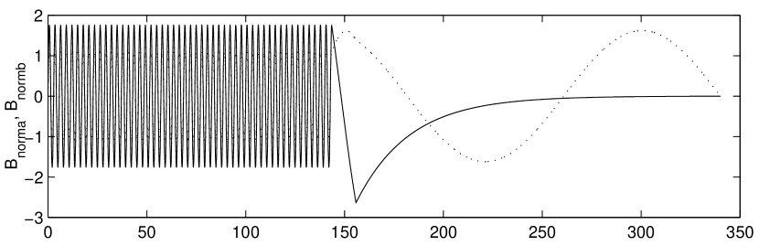
Figure 1: Mode-profiles for the eigenmodes are shown for the parameter values $n_{1}=1.22$, $n_{2}=1.0005$, $l_{1}m/x_{0}=143$, $l_{2}m/x_{0}=12.3$ and $l_{3}m/x_{0}=184$. $B_{{\rm norm}\,a}$ is the solid line and $B_{{\rm norm}\,b}$ is the dotted line, and $I_{c}=0.27$.

We define the eigenmodes to have the form $\widetilde{B}_{za,b}=\widetilde{B}_{a,b}(t)B_{{\rm norm}a,b}(z,y,z)$, where $\widetilde{B}_{a,b}$ is a time-dependent amplitude and the normalized eigenmodes $B_{{\rm norm}a,b}$ satisfy $\int_{V}\left|B_{{\rm norm}a,b}\right|^{2}dV=V$. We let all electromagnetic field components be of the form $A=A_{a}(\boldsymbol{r})\exp(-i\omega_{a}t)+A_{b}(\boldsymbol{r})\exp(-i\omega_{b}t)+\mathrm{c.c.}$, where c.c. stands for complex conjugate, and the indices stand for the eigenmodes discussed above. The gravitational perturbation can be approximated by $h_{+,\times}=\widehat{h}_{+,\times}\exp(-i\omega_{g}t)+\mathrm{c.c}$, where we neglect the spatial dependency, since the gravitational wavelength is assumed to be much longer than all of the cavity dimensions. During a certain interval in time, the frequency matching condition $\omega_{b}=\omega_{a}+\omega_{g}$ will be approximately fulfilled. Given the wave equation (1), and the above ansatz we find after integrating over the length of the cavity

$$\frac{2i\omega_{b}}{c^{2}}\left(\frac{\partial}{\partial t}-\gamma\right)\widetilde{B}_{b}=-h_{+}k_{1a}^{2}\widetilde{B}_{a}I_{c},$$ (2cd)

where

$$I_{c}=\frac{1}{Vk_{1a}^{2}}\int_{V}\frac{\partial^{2}B_{{\rm norm}\,a}}{\partial z^{2}}B_{{\rm norm}\,b}\,dV,$$ (2ce)

and we have added a phenomenological linear damping term represented by $\gamma$. Thus we note that for the given geometry, only the $h_{+}$-polarization gives a mode-coupling. Calculations of the eigenmode parameters show that $I_{c}$ may be different from zero when $n_{1,2}\neq 1$, and generally $I_{c}$ of the order of unity can be obtained, see fig. 1 for an example. From Eq. (2cd), we find that the saturated value of the gravitationally excited mode is

$$\left|\widetilde{B}_{b{\rm sat}}\right|=\frac{h_{+}k_{1a}^{2}c^{2}\widetilde{B}_{a}}{2\gamma\omega_{b}}I_{c}\ .$$ (2cf)

In fig. 1 it is shown that we can get an appreciable mode-coupling constant $I_{c}$ for a cavity filled with materials with different dielectric constants, and it is of interest whether or not this can be achieved in a vacuum cavity. As seen by Eq. (2ce), the coupling is essentially determined by the wave numbers of the modes, given by $k=(m^{2}\pi^{2}/x_{0}^{2}-n^{2}\omega^{2}/c^{2})^{1/2}$. Thus by adjusting the width $x_{0}$ in a vacuum cavity, we may get the same variations in the wave numbers as when varying the index of refraction $n$. The translation of our results to a vacuum cavity with a varying width is not completely accurate, however. When varying $x_{0}$, the mode-dependence on $x$ and $z$ does not exactly factorize, in particular close to the change in width. Moreover, the contribution to the coupling $I_{c}$ in each section becomes proportional to the corresponding volume, and thereby also to the cross-section. However, since most of the contribution to the integral in Eq. (2ce) comes from region 1, our results can still be approximately translated to the case of a vacuum cavity, by varying $x_{0}$ instead of $n$ such as to get the same wavenumber as in our above example.

We denote the minimum detection level of the excited mode with $\widetilde{B}_{b\min}$ and the maximum allowed field in the cavity with $\widetilde{B}_{a\max}$. The magnetic field $\widetilde{B}_{b\min}$ is related to the minimum number of photons $N_{bm}$ needed for detection by $\widetilde{B}_{b\min}\sim\left(N_{bm}\mu_{0}\omega_{b}\hbar/x_{0}y_{0}l\right)^{1/2}$. Furthermore, we have $2\gamma\omega_{b}/k_{1a}^{2}c^{2}$ $\simeq(1/3Q)(\omega_{b}^{2}/k_{1a}^{2}c^{2})\simeq 2/3Q$, where $Q=\omega_{b}/2\pi\gamma$ is the quality factor of the cavity, and thus we obtain, using Eq. (2cf),

$$h_{\min}\sim\frac{2}{3QI_{c}\widetilde{B}_{a\max}}\left(\frac{\mu_{0}\omega_{b}\hbar N_{bm}}{x_{0}y_{0}l}\right)^{1/2}.$$ (2cg)

Before giving estimates of the parameter values, we will investigate certain other effects that may limit the detection efficiency.

Massive binaries produce monochromatic radiation to a good approximation, but close to merging, the frequency will be increasing rather rapidly which means that the phase matching will be lost. The cavity is designed to detect the frequency $\omega_{g}$, and we have assumed that the signal varies as $\exp(-{\rm i}\omega_{g}t)$, but in reality we have $\exp(-{\rm i}\psi(t))$, where for simplicity we assume $\psi=0$, $d\psi/dt=\omega_{g}$ at $t=0$. The coherence time $t_{{\rm coh}}$ is roughly defined by $\omega_{g}t_{{\rm coh}}-2\psi(t_{{\rm coh}}/2)=\pi$. Thus, $t_{{\rm coh}}\approx[2\pi/(d\omega_{g}/dt)]^{1/2}$ provided $\omega_{g}t_{\rm coh}\gg 1$. Using Newtonian calculations of two masses $M$ in circular orbits around the center of mass, complemented by the quadrupole formula for gravitational radiation, we find

$$\frac{d\omega_{g}}{dt}=\frac{388\omega_{g}^{2}}{5c^{5}}\left(\frac{GM\omega_{g}}{8}\right)^{5/3}.$$ (2ch)

Close to binary merging, the time of coherent interaction will be shorter than the photon life time, and in that regime the growth of the excited mode is limited by decoherence rather than the damping due to a finite quality factor of the cavity. However, formula (2cg) can still be applied if we simply replace $Q$ by $\omega_{b}t_{{\rm coh}}$.

To be able to estimate the number of photons needed for detection, we must study various sources of noise. The simplest effect is direct thermal excitation of photons in mode $b$. Since each mode has a thermal energy level of order $KT$, the number of such photons is $\sim KT/\hbar\omega_{b}$. However, we will also have a contribution associated with thermal variations in the length of the cavity. A standard model for the variations in length $\delta l$ is [6]

$$\frac{d^{2}\delta l}{dt^{2}}+\frac{\omega_{l}}{Q_{mec}}\frac{d\delta l}{dt}+\omega_{l}^{2}\delta l=-l\omega_{g}^{2}h_{+}\exp(i\omega_{g}t)+a_{th},$$ (2ci)

where $\omega_{l}$ is the eigenfrequency of longitudinal oscillations (of the order of the acoustic velocity in the cavity divided by the length), $Q_{mec}$ is the mechanical quality factor associated with these oscillations, and $a_{th}$ is the stochastic acceleration due to the thermal motion, giving rise to a random walk in the oscillation amplitude. First we note that the amplitude of the length variations with the gravitational frequency is $\delta l_{g}=\omega_{g}^{2}h_{+}/(\omega_{g}^{2}-\omega_{l}^{2})$. We will consider the case when $\omega_{l}^{2}\sim 2\omega_{g}^{2}$, which implies that the amplitude of the gravitational length perturbation is essentially unaffected by the restoring force of the cavity, as is the number of gravitationally generated photons.

The thermal fluctuation contribution to the right hand side of Eq. (2cd), via the coupling to the pump wave, becomes proportional to $\delta l_{th}\exp[i(\omega_{b}-\omega_{a})t]$. Since $\delta l_{th}\sim\exp(i\omega_{l}t)$, the longitudinal oscillations give rise to slightly off-resonant (i.e., driven) fields with a frequency difference $\delta\omega=\omega_{l}-\omega_{g}$ compared to mode $b$. However, due to the stochastic changes in amplitude and/or phase of the longitudinal oscillation (where the time-scale for significant changes is given by $\tau\sim Q_{mec}/\omega_{l}$), a contribution to mode $b$ of the order $\left\langle{\delta l_{th}}\right\rangle\sqrt{\omega_{l}/\delta\omega Q_{mec}}\,dt\sim\sqrt{KT/m\omega_{l}^{2}}\sqrt{1/Q_{mec}}\,(2\pi/\delta\omega)$ is also made during a single oscillation period $dt=2\pi/\delta\omega$. Here $m$ is the mass taking part in the longitudinal oscillation. During a time of the order $t_{coh}$, this contribution adds up to approximately $(\sqrt{2\pi}/\delta\omega)\sqrt{KT/m\omega_{l}^{2}}\sqrt{\delta\omega t_{coh}/Q_{mec}}$ by a random walk process. Using $\delta\omega\sim\omega_{g}$, the condition for the gravitational contribution $\sim hlt_{coh}$ to be larger than that of the thermal fluctuations can be written

$$h_{min}>\frac{2\pi}{\omega_{l}l}\sqrt{\frac{KT}{m}}\frac{1}{\sqrt{Q_{mec}\omega_{g}t_{coh}}}.$$ (2cj)

Assume that we want to reach a sensitivity $h_{min}\approx 7\times 10^{-23}$. We let $x_{0}=0.1\,\mathrm{m}$, $y_{0}=0.2\,\mathrm{m}$, $l=4\,\mathrm{m}$ , and $m=4$ which gives $\omega_{b}\approx 4\pi c/x_{0}=4\times 10^{10}\,\mathrm{rad/s}$. Furthermore, we take $\omega_{g}=1000\,\mathrm{rad/s}$ and let $\omega_{l}=1500\,\mathrm{rad/s}$. We assume $T=1\,\mathrm{K}$ together with $m=2500\,\mathrm{kg}$. From (2cj), we then find that we need a mechanical quality factor $Q_{mec}\approx 6\times 10^{7}$ to reach the desired sensitivity. Moreover, assuming the necessary number of photons for detection to be $N_{bm}=20$ (well above the direct electromagnetic noise level of a few photons), $I_{c}\approx 0.3$ and $\widetilde{B}_{a\max}=0.2\,\mathrm{T}$ [11, 12], we need an electromagnetic quality factor $Q=5\times 10^{9}$ to reach the desired sensitivity $h_{\min}\approx 7\times 10^{-23}$. Note that the coherence time is slightly longer than the photon life-time, as needed.

Following the example given above for calculating the coherence time, i.e., a binary consisting of two compact objects, each of one solar mass $M_{\odot}$, separated by a distance $d$, the amplitude of the metric perturbation at a distance $r$ is given by $h\approx 2G^{2}M^{2}/c^{2}rd$. For definiteness we choose $d=80\,{\rm km}$ corresponding to $\omega_{g}=1000\,\mathrm{rad/s}$, and thus for $h_{\min}$ of the order of $7\times 10^{-23}$ we obtain the maximum observational distance $r_{\max}\approx 8\times 10^{7}\,{\rm ly}$. Using data from Ref. [17], we deduce that the number of galaxies within the observational distance $r_{\max}\sim 10^{8}\,\mathrm{ly}$ is of the order $N=10^{5}$. Combining these figures with the expected number of compact binary mergers per galaxy and million years [13], we obtain a detection rate in the interval $1-20$ events per year (the uncertainty is due to different models used for the birth of compact binaries).

Our proposal for a gravitational wave detector is to a large extent based on currently available technology [18, 10, 11, 12], and our requirements are moderate given the performance of some existing microwave cavities. For example, values of $Q\approx 4\times 10^{10}$ has been reported in Ref. [10] and quantum non-demolition measurements of single microwave photons have been made in Ref. [18]. Furthermore, the key performance parameters of the superconducting niobium cavities, i.e., the quality factor and the maximum allowed field strength before field emission, have been improving over the years, suggesting that the detection sensitivity can be increased even further.

A sensitivity $h_{\min}\lesssim 10^{-22}$ seems extremely good, but, on the other hand, idealizations have been made when making the estimate. In addition to any effects induced by the gravitational wave, the walls generally vibrate slightly due to the electromagnetic forces exerted by the large pump field. While these later oscillations clearly will be larger than the variations in length that are directly due to the gravitational wave, the associated nonlinearities will be harmonics of the pump frequency, and thus such effects do not couple to the other eigenmodes of the cavity. Furthermore, we have assumed that the detection of the excited mode is not much affected by the presence of the pump signals. Even though mode $a$ is partially filtered out in region 3, the small frequency shift between the two electromagnetic modes may pose a certain difficulty in this respect: In particular, a very narrow bandwidth (pump) antenna signal must be used, in order to exclude the slightest initial perturbation at the gravitationally excited frequency $\omega_{b}$.

However, although there are technical difficulties in constructing an electromagnetic detector, the real advantage is the possibility to reduce the size of the devise. In the example presented above, the length of the cavity has been taken to be $4\,\mathrm{m}$, and the cross section roughly $1/50\,\mathrm{m}^{2}$. This alone could prove to be useful when trying to set up new gravitational wave observatories.

References

References

- [1] Taylor J H 1994 Rev. Mod. Phys. 66 711
- [2] Schutz B F 1999 Class. Quantum Grav. 16 A131
-
[3]
URL http://www.ligo.caltech.edu/;
URL http://www.virgo.infn.it/;
URL http://www.geo600.uni-hannover.de/; URL http://tamago.mtk.nao.ac.jp/; URL http://www.gravity.uwa.edu.au/AIGO/AIGO.html; URL http://sam.phys.lsu.edu/; URL http://www.auriga.lnl.infn.it/; URL http://www.gravity.uwa.edu.au/bar/bar.html - [4] URL http://lisa.jpl.nasa.gov/
- [5] Braginskiĭ V B and Menskii M B 1971 Zh. Eksp. Teor. Fiz. Pis’ma 13 585 [1971 JETP Lett. 13 417]; Lupanov G A 1967 Zh. Eksp. Teor. Fiz. 52 118 [1967 Sov. Phys.-̇J̇ETP 25 76]; Braginskiĭ V B et al 1973 Zh. Eksp. Teor. Fiz. 65 1729 [1974 Sov. Phys. - JETP 38 865]; Grishchuk L P and Sazhin M V 1975 Zh. Eksp. Teor. Fiz. 68 1569 [1976 Sov. Phys. - JETP 41 787]; Balakin A B and Ignat’ev Yu G 1983 Phys. Lett. A 96 10; Kolosnitsyn N I 1994 Zh. Eksp. Teor. Fiz. Pis’ma 60 69 [1994 JETP Lett. 60 73]; Cruise A M 2000 Class. Quantum Grav. 17 2525; URL http://www.sr.bham.ac.uk/research/gravity
- [6] Grishchuk L P and Polnarev A G 1980 General Relativity and Gravitation Vol. 2, ed. A Held, (Plenum Press); Grishchuk L P et al 2001 Usp. Fiz. Nauk 171 3 [2001 Phys. Usp. 44 1]
- [7] Pegoraro F, Picasso E and Radicati L A 1978 J. Phys. A: Math. Gen. 11 1949; Pegoraro F, Radicati L A, Bernard P and Picasso E 1978 Phys. Lett. A 68 165; Caves C M 1979 Phys. Lett. B 80 323
- [8] Brodin G and Marklund M 1999 Phys. Rev. Lett. 82 3012; Servin M et al 2000 Phys. Rev. E 62 8493
- [9] Reece C E, Reiner P J and Melissinos A C 1984 Phys. Lett. A 104 341; Reece C E, Reiner P J and Melissinos A C 1986 Nucl. Instr. Meth. A 245 299
- [10] Varcoe B T H et al 2000 Nature 403 743; Brattke S, Varcoe B T H and Walther H 2001 Phys. Rev. Lett. 86 3534
-
[11]
Graber J 1993 PhD Dissertation (Cornell university),
see also http://w4.lns.cornell.edu/public/CESR/SRF/BasicSRF/SRFBas1.html - [12] Aune B et al 2000 Phys. Rev. ST AB 3 092001
- [13] Belczynski K, Kalogera V and Bulik T 2002 Astrophys. J. 572 407
- [14] Marklund M, Brodin G and Dunsby P K S 2000 Astrophys. J. 536 875
- [15] Anile A M 1989 Relativistic fluids and magneto-fluids (Cambridge Univ. Press, Cambridge)
- [16] Braginskiĭ V B and Rudenko V M 1978 Phys. Rep. 46 165
- [17] Kalogera V, Narayan R, Spergel D N and Taylor J H 2001 Astrophys. J. 556 340
- [18] Nogues G et al 1999 Nature 400 239