The Munich Near-Infrared Cluster Survey – IV. Biases in the Completeness of Near-Infrared Imaging Data

Abstract

We present the results of completeness simulations for the detection of point sources as well as redshifted elliptical and spiral galaxies in the $K^{\prime}$-band images of the Munich Near-Infrared Cluster Survey (MUNICS). The main focus of this work is to quantify the selection effects introduced by threshold-based object detection algorithms used in deep imaging surveys. Therefore, we simulate objects obeying the well-known scaling relations between effective radius and central surface brightness, both for de Vaucouleurs and exponential profiles. The results of these simulations, while presented for the MUNICS project, are applicable in a much wider context to deep optical and near-infrared selected samples. We investigate the detection probability as well as the reliability for recovering the true total magnitude with Kron-like (adaptive) aperture photometry. The results are compared to the predictions of the visibility theory of Disney and Phillipps in terms of the detection rate and the lost-light fraction. Additionally, the effects attributable to seeing are explored. The results show a bias against detecting high-redshifted massive elliptical galaxies in comparison to disk galaxies with exponential profiles, and that the measurements of the total magnitudes for intrinsically bright elliptical galaxies are systematically too faint. Disk galaxies, in contrast, show no significant offset in the magnitude measurement of luminous objects. Finally we present an analytic formula to predict the completeness of point-sources using only basic image parameters.

1 Introduction

The luminosity function as well as the mass function, and to a lesser degree the number counts of galaxies provide an important observational toolset for understanding the evolution of galaxies. Due to their statistical nature, these methods rely on the understanding of sample selection effects, i.e. the knowledge of what fraction of the true number of galaxies, as a function of their intrinsic properties, is actually present in the sample. In order to extract this information from the data, two different approaches are commonly used in the literature, creation of artificial objects or modification of observed objects.

The synthetic objects are, as described by e.g. Martini (2001), usually point-sources or objects with galactic profiles, that are inserted into the observed images. Then the fraction of objects recovered by the applied detection algorithm as a function of, e.g, the assigned apparent magnitude is computed. This approach exhibits two major drawbacks: The galaxies are created using a discrete set of half-light radii and a continuous range of magnitudes, thus ignoring known relations between surface-brightness and effective radius, like the fundamental plane (Bender et al., 1992; Gavazzi et al., 2000). The results show the completeness limits for distinct types of objects, but as the actually observed ratio of these types is unknown, predictions about the total completeness of the data cannot be made.

In the second case, as conducted by e.g.Bershady et al. (1998), Arnouts et al. (1999) or Saracco et al. (1999), images of the observed objects are dimmed or brightened to produce artificial objects. The advantage of this approach is, that it preserves the observed mix of galaxies, assuming that it remains unchanged with time, yet the resulting completeness fractions for extended objects are questionable, as long as the resolution of images is seeing-limited. When the bright extended objects are dimmed, they are still profile dominated, whereas in reality a faint object would be seeing dominated. The same holds true for artificially brightened faint sources. The resulting objects would still be seeing dominated. Furthermore, the observed size of a local object of given magnitude is different from the size of a distant object of the same brightness. Consequently this method only yields information about the probability to detect an object if it was fainter, but not about the probability to detect an intrinsically faint object.

Another drawback of both approaches is that the obtained results can only be used to define the completeness of the survey in apparent magnitudes. The magnitudes and radii of the artificially constructed objects all are physically plausible, but the objects do not occupy one plane in the $\langle\mu_{e}\rangle-r_{e}-z$ parameter space. Therefore the results derived using galactic profiles are not usable to correct absolute magnitudes, as effects of the completeness of different galaxy types at given redshifts are unknown.

In deep extra-galactic surveys, the observed galaxies span a wide range in intrinsic profile shape, intrinsic brightness, and intrinsic size. The apparent quantities vary with cosmological distance, such that the fraction of galaxies visible is also a function of redshift. The need to simulate objects obeying the known scaling relations for galaxies was pointed out several times in the literature. Using profiles obeying the magnitude-radius relations, Yoshii (1993) predicted the number of objects lost in number count analysis. He finds a strong dependence of the detection rate on the applied detection criteria and magnitude measurement algorithm, leading to a larger number of undetected faint galaxies at high redshifts.

Dalcanton (1998) analysed the biases of the luminosity function introduced by the cosmological effects of size variation with redshift, and cosmological dimming for galactic profiles in dependence of size and magnitude, taking into account effects of seeing. Starting from the deficiency that magnitudes are usually measured as some sort of isophotal magnitude, that is directly influenced by the above mentioned effects, she finds the possibility of a severe underestimation of the true luminosity function introduced by the fact that an object and distance dependent part of the light is lost outside the limiting isophote.

The simulations presented in this paper were performed by adding artificially created objects into the $K^{\prime}$-band images of the Munich Near-Infrared Cluster Survey (MUNICS; Drory et al., 2001). We analysed the detection probability and the reliability for recovering the assigned magnitude for point-like sources (Moffat profiles), elliptical galaxies (de Vaucouleurs profiles), and spiral galaxies (exponential profiles). The radii and magnitudes of the simulated galaxies were distributed according to the projected fundamental-plane relation (Bender et al., 1992) for ellipticals and a Freeman law type relation (Freeman, 1970) constructed from observed data for spirals. The galaxies were simulated at five distinct redshifts between $z=0.5$ and $z=1.5$, taking into account size variation with redshift as well as cosmological dimming and K-correction. A flat universe with $\Omega_{M}=0.3$, $\Omega_{\Lambda}=0.7$ and $H_{0}=65$ km s^-1 Mpc^-1 was assumed.

The results of the completeness simulations for the different fields of the MUNICS survey presented here, illustrate the principal limitations of imaging surveys. A full correction of the incompleteness would only be possible if the type mix of galaxies was known. The presentation of the results here is limited to the $K^{\prime}$-band data, but as the selection biases are caused by the physical nature of the objects, they are applicable in a much wider context to deep extragalactic surveys spanning the optical and near-infrared wavelength regimes. The conclusions drawn here result from the use of a threshold-based detection algorithm. Accordingly they will hold true for other similarly created datasets as well.

Finally, a reliable and handy analytic formula to estimate the completeness limit of a survey for point-like sources is presented. In Section 2 the implementation of the simulations and the generation of the artificial objects is described. Section 3 presents the results of the simulations, and a discussion of these. To compare the results with analytic predictions, we present the results of an analysis using the visibility theory devised by Disney & Phillipps (1983) in Section 4 for the detection probability and in Section 5 for the lost-light fraction. In Section 6 we discuss the effects of seeing in the above mentioned analysis. Finally, in Section 7 we present the results of the completeness simulations for the MUNICS fields.

1.1 The Munich Near-Infrared Cluster Survey (MUNICS)

The Munich Near-Infrared Cluster Survey (MUNICS) is a wide-field medium-deep survey in the near-infrared $K^{\prime}$ and $J$ pass-bands (Drory et al. 2001; MUNICS1 hereafter). The survey consists of a $K^{\prime}$-selected catalogue down to $K^{\prime}\leq 19.5$ covering an area of 1 square degree. Additionally, 0.35 square degrees have been observed in $I$, $R$, and $V$. The layout of the survey, the observations and data reduction are described in Drory et al. (2001).

2 Implementation of the simulations

Detection probabilities and photometry results were analysed for three different profile shapes: de Vaucouleurs profiles, exponential disks and point-like sources.

For each profile type and each image, 200 artificially created objects were added to the image, taking into account the noise properties of the background and the photometric zero-point. The resulting image was processed in the same way as described in MUNICS1 regarding detection and photometry, using the software package YODA (Drory, 2002). The resulting object catalogue was used to calculate the fraction of recovered objects and to compare the resulting photometry in Kron-like elliptical apertures to the quantities in the input catalogue.

This procedure was repeated 500 times resulting in a total of 100 000 artificial objects per type. In each run, the artificial objects were distributed randomly in (x,y)-position across the image, excluding a 25 pixel wide strip along the image borders, and requiring 20 pixel distance to existing objects, as we intentionally avoid crowding which would introduce effects beyond the scope of this work. Extended sources were convolved with a Gaussian with a FWHM of the measured seeing in the image. Poisson noise was added to all profiles. In the following we discuss the generation of objects of each of the examined profile types in more detail.

2.1 Stars and point-sources

Point-like sources were simulated using a Moffat profile (Moffat, 1969) of the form

$$I(r)=\frac{I_{c}}{\left(1+\left(\frac{r}{R}\right)^{2}\right)^{\beta}}.$$ (1)

with the characteristic intensity $I_{c}$. The size parameter $R$, defining the radius of the created object, was set to the measured value from point-like real sources in the analysed image, and the Moffat parameter $\beta$ was fixed at the canonical value of $2.5$. The apparent magnitudes assigned to the point-sources were chosen randomly from a constant probability density in the range $15\leq m_{K^{\prime}}\leq 25$.

2.2 Elliptical galaxies

Elliptical galaxies were simulated using a de Vaucouleurs profile (de Vaucouleurs, 1948). For a galaxy with effective radius $r_{e}$ and effective intensity $I_{e}$ (defined as the intensity at $r_{e}$), this profile can be written as

$$I(r)=I_{e}\exp\left(-7.67\left(\frac{r}{r_{e}}\right)^{\frac{1}{4}}\right).$$ (2)

For the sake of simplicity an $r^{1/4}$ law is applied, ignoring relations between luminosity and the shape of the profile. But it should be kept in mind, that an $r^{1/n}$ profile with $n>4$ would show the same biases as described here. To create a realistic population of elliptical galaxies, the radii and absolute magnitudes of the galaxies were distributed according to the Kormendy relation (Kormendy, 1985), a projection of the local fundamental-plane relation (Burstein et al., 1997). We used the $K$-band Kormendy relation published by Pahre et al. (1995) for the effective radius of the galaxy $R_{e}$ in kpc and the mean effective surface brightness $\langle\mu_{e}\rangle$ in mag arcsec^-2

$$\log R_{e}=0.332\langle\mu_{e}\rangle-5.090.$$ (3)

Using the definition of $\langle\mu_{e}\rangle$

$$m=-1.995-5\log r_{e}+\langle\mu_{e}\rangle.$$ (4)

equation (3) can be transformed into a relation between absolute magnitude $M$ and effective radius $R_{e}$

$$M_{K^{\prime}}=-1.99\log R_{e}-23.235.$$ (5)

The absolute magnitudes were chosen randomly and uniformly in the range $-26.5\leq M_{K^{\prime}}\leq-20.5$, corresponding to a range of $\pm 3$ magnitudes around $M_{K}^{*}$ for the local K-band luminosity function (Loveday, 2000).

To simulate a galaxy at redshift $z$, the apparent radius was calculated from the given physical radius using the angular distance, and the absolute magnitude was transformed into the apparent magnitude using the luminosity distance. During each repetition of the simulation 40 galaxies for each of the five redshifts $z\in\{0.5,0.75,1.0,1.25,1.5\}$ were created. The axis ratios $e$ were selected randomly in the range $0.7\leq e\leq 1.0$, the position angles were chosen arbitrarily. For the galaxies at $z=0.5$ the absolute magnitude range was shifted $-25.5\leq M_{K^{\prime}}\leq-19.5$ to better trace the faint-end drop-off of the completeness curve. The resulting apparent magnitudes were adjusted using only K-corrections derived from model SEDs from Bender (2001). The used values are listed in Table 1. Possible effects introduced by luminosity evolution with redshift were explored, and are discussed at the end of section 3.

$z$	de Vaucouleurs	exponential
$0.5$	$-0.63$	$-0.68$
$0.75$	$-0.73$	$-0.83$
$1.0$	$-0.84$	$-0.97$
$1.25$	$-0.88$	$-1.03$
$1.5$	$-0.87$	$-1.02$

Table 1: K-corrections in magnitudes for de Vaucouleurs and exponential profiles applied in the simulations. The values were derived from empirical SEDs (Bender, 2001).

2.3 Spiral galaxies

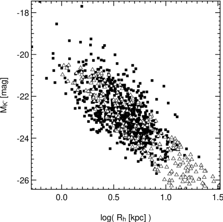
Figure 1: Absolute $K^{\prime}$-band Magnitudes $M_{K}^{\prime}$ and effective radii for the galaxies fitted by a pure exponential profile published by Gavazzi et al. (2000) (filled squares) and some during the simulations created artificial objects (open triangles).

Spiral galaxies were simulated as pure exponential profiles with no bulge component. An analysis of the bulge-disk decomposition for the galaxies published by Gavazzi et al. (2000) shows that the contribution of the bulge to the total luminosity is less than 18%. We therefore neglect the contribution of the bulge.

For a galaxy with half-light radius $r_{h}$ and central intensity $I_{e}$ the intensity profile can be written as

$$I(r)=I_{0}\exp\left(-1.6783\frac{r}{r_{h}}\right).$$ (6)

To create objects with realistic magnitude-size ratios, all galaxies fitted by a pure exponential profile from $H$-band surface photometry data of spiral galaxies published by Gavazzi et al. (2000) were used. The absolute $H$-band magnitudes were transformed into the $K^{\prime}$-band using $H-K^{\prime}$ colours derived from empirical SEDs presented in Bender (2001). The mean correction was $H-K^{\prime}\simeq 0.128$ mag. Using the objects’ distances, the half-light radii in kpc $R_{H}$ were computed from the published values. The resulting distribution of galaxies in the $\log R_{h}-M_{K^{\prime}}$ plane was then approximated by assuming

$$M_{K^{\prime}}=-5\left(\log R_{h}\pm 0.25\right)-19.7.$$ (7)

For a population of local spiral galaxies, this distribution would be analogous to a Freeman law with a $K^{\prime}$-band central surface brightness of $17.52$ mag arcsec^-2 and an rms of $1.73$ mag.

Fig. 1 shows the absolute magnitudes and effective radii of the Gavazzi et al. data and of some artificially created objects. The distribution of the artificial objects reproduces that of the observed population reasonably well, extending to somewhat brighter magnitudes.

The absolute magnitudes of the objects were randomly chosen in the range $-26.5\leq M_{K^{\prime}}\leq-20.5$, again corresponding to a range of $\pm 3$ magnitudes around $M^{*}_{K}$ for a local K-band luminosity function (Loveday, 2000). Using the same techniques as for the elliptical galaxies, the spirals were simulated for the same five redshifts, with axis ratios in the range $0<e\leq 1$ and arbitrary position angles. The resulting apparent magnitudes were adjusted using only K-corrections derived from model SEDs shown in Bender (2001), no evolution corrections were applied. The results of tests for influences of luminosity evolution are discussed at the end of section 3. The applied values are listed in Table 1. The mean surface brightnesses $\langle\mu\rangle$ were derived from a sample of local spiral galaxies. Brightness evolution with redshift would make the galaxies brighter, while the radii are known not to change significantly up to redshifts of $z\sim 1$.

3 Results and Discussion

Figure 2: Probability $P_{D}(m)$ to re-detect an artificially created point-source (upper panel), an extended object with a de Vaucouleurs profile (middle panel) or exponential profile (lower panel) as a function of the objects’ $K^{\prime}$-band input magnitude $m_{K^{\prime}}$. The different line types in the middle and lower panel show the completeness for the five analysed redshifts: $z=0.5$ (solid), $0.75$ (dash), $1.0$ (dot), $1.25$ (dashdot) and $1.5$ (dashdotdot).

Figure 3: Mean magnitude difference $\delta m=m_{K^{\prime}}-m_{meas}$ between the assigned magnitude $m_{K^{\prime}}$ of an object and the Kron-magnitude measured by the photometry software $m_{meas}$ in bins of $0.25$ mag as a function of the input $K^{\prime}$-band magnitude $m_{K^{\prime}}$. The top panel shows the results for point-sources, the middle panel for de Vaucouleurs profiles and the lower panel for exponential profiles. The errorbars show the standard deviation of $\delta m$

The results for one of the MUNICS fields with a seeing of approximately one arcsec FWHM are shown in Fig. 2. The upper panel shows the results for the point-sources, the middle and the lower panel for the de Vaucouleurs and exponential profiles, respectively, for the five redshifts simulated. An interesting effect seen in the figure is that, for higher redshifts $z\ga 1$, the detection probability does not reach unity even for the brightest objects, forming a plateau at some lower value. This effect is mainly caused by the cosmological surface brightness dimming and discussed in detail in Section 3 below. Fig. 2 shows that the completeness for point-like sources provides a rough but reasonable approximation for the completeness of the analysed extended objects up to a redshift of $z=1.0$.

For each detected object, the difference between the input magnitude and the measured Kron-magnitude was computed. Fig. 3 shows the mean magnitude differences for the analysed profiles, averaged in bins of 0.25 mag and with the standard deviation of the measurements in the bin indicated as errorbars.

The object recovery probabilities for the high-redshift de Vaucouleurs profiles, and to a lesser degree for the exponential profiles exhibit a significant detection bias compared to lower redshift objects, as shown in Fig. 2. The fact that the objects at these redshifts never reach a detection probability of one is caused by the distribution of their physical parameters along the fundamental-plane relation – in case of the ellipticals – and according to the Freeman law – in case of the disks. In both cases, as the object’s size increases its radius grows and therefore the average surface brightness decreases. As a result, even the brightest objects of the distribution fail to produce a large enough area above the threshold in surface brightness to be detected with high probability in the presence of noise. In Section 4 these results are compared with the theoretical predictions of the visibility theory, which will confirm the above statement.

The detection deficiencies at low redshifts found for the exponential profiles are caused by the flat light distribution of the objects, resulting in a low central surface brightness even for the luminous objects. The image noise can then scatter these objects below the detection threshold. This result is in general agreement with the predictions of McGaugh et al. (1995). In their paper they re-derive the formalism devised by Disney & Phillipps (1983) using two parameters for the disk galaxies. They predict that disk galaxies would suffer from detection biases introduced by their low central surface brightness.

Martini (2001) performed simulations similar to the ones presented here, analysing the detection probabilities of Moffat, de Vaucouleurs and exponential profiles. The galactic profiles were created for a discrete set of half-light radii and a continuous range of apparent magnitudes. The simulations show a decrease of the limiting magnitude with increasing half-light radius. This effect can be found in the simulations presented here, by comparing the completeness magnitude at different redshifts. With increasing redshift, the sampled range in absolute magnitudes is shifted toward fainter apparent magnitudes, resulting in an increase of effective radius at given apparent magnitude. The detection bias against high redshifted elliptical galaxies we showed cannot be found by the simulations performed by Martini, as these effects are only visible when distributing the objects along a fundamental-plane relation.

The bias first shown by Disney & Phillipps (1983), that with increased distance more low-luminosity system would be lost from the survey, is reproduced by our simulations as well. With increasing redshift, the magnitude of the completeness limit stays approximately constant, or gets brighter, while the range of sampled absolute magnitudes is shifted to fainter apparent magnitudes. This means, that with increasing redshift, the observable range in absolute magnitudes moves toward higher luminosities, the low-luminosity systems become unobservable.

Figure 4: Intensity integrated over image pixels for a de Vaucouleurs profile (solid line) and an exponential profile (dashed line) at redshift $z=0.5$ with similar total magnitude and effective radius. The upper left panel shows the case in the absence of seeing, the upper right one, with a seeing of $0.5$ arcsec and the lower left with a seeing of $1.6$ arcsec. Plotted is the logarithm of the intensity against the radius relative to the effective radius.

The deviations of the measured magnitude from the true magnitude for the de Vaucouleurs profiles as seen in Fig. 3, can be explained as resulting from the estimate of the Kron-like aperture radius under the conditions of a surface brightness limited detection procedure and the involved intrinsic brightness profile of the objects. The upper left panel of Fig. 4 shows the intensity of a de Vaucouleurs and an exponential profile with similar total magnitude and effective radius, as a function of the radius in units of the effective radius in absence of seeing. Assuming that both profiles are detected at a similar intensity level, the Kron-radius of the de Vaucouleurs profile would be smaller compared to the exponential profile, even though the effective radius of both objects is the same. The measured light within the underestimated radius results then in a too faint object magnitude. Combined with the previously mentioned surface brightness distribution along the fundamental plane, this leads to an increased amount of lost flux and a larger error in the output magnitude for brighter objects, as these have lower surface brightnesses. In Section 5 we will confirm this explanation with predictions based on computations of the visibility function and the lost-light fraction.

Our results confirm the predictions of McGaugh (1994), that the magnitudes of distant spiral galaxies would be measured correctly for luminous galaxies, and slightly underestimate them for the systems with low-luminosity.

The deviations of the measured from the input magnitude we find, are compatible with the simulations of Martini (2001), who compared the reliability of different photometric methods for point-sources and exponential profiles. For Kron-like magnitude measurements both shapes would be measured correctly at the bright end, and slightly underestimated at the faint end.

Figure 5: Results of a simulation assuming luminosity evolution with redshift. Shown are the simulation results for de Vaucouleurs profiles (left column) and exponential profiles (right column) at a redshift $z=1$ for a seeing of $0.8"$ (upper row) and $1.6"$ (lower row). The solid curve shows the results obtained from the normal simulations, the dashed line for a simulation with objects brightened artificially by $0.75$ mag.

To explore the effects caused by the increase of the objects’ surface brightness introduced by luminosity evolution with redshift, an additional set of simulations for objects at $z=1$ was created. The brightnesses of the created artificial de Vaucouleurs and exponential profiles was increased by $0.75$ magnitudes (de Propris et al., 1999). The results shown in Fig. 5 show no significant change of the magnitude of the 50% completeness limit. The reason for this is that the increase of the detectable area is small in the magnitude range of the 50% limit. The increase in size is larger for brighter magnitudes, but the positive effect is mainly lost due to the already high detection probability, or may result in a slightly higher plateau level.

4 Visibility theory

Figure 6: Area above detection threshold for point-sources with Moffat profiles. The upper panel shows the predictions derived from the visibility theory (Disney & Phillipps, 1983). The thick solid histogram shows the area above the detection threshold integrated over the image pixels in presence of seeing. The smooth dashed line gives the area above the surface brightness limit as predicted by the inversion of the profile. The thin horizontal line is the area of the minimum number of connected pixels needed to detect an object. The lower panel shows the object recovery probability as a function of assigned input magnitude.

Figure 7: Predictions of the visibility function in comparison with the results of completeness simulations for de Vaucouleurs profiles (upper row) and exponential profiles (lower row) at redshift $z=0.5$ (left column) and $z=1.25$ (right column). The upper panel of each plot depicts the area above detection threshold. The thin solid line shows the area above the detection threshold integrated over the image pixels in absence of seeing, the thick solid line the same but in presence of appropriate seeing. The smooth dotted curve gives the area above the surface brightness limit in absence of seeing, the dashed line in presence of seeing. The thin horizontal line is the area of the minimum number of connected pixels needed to detect an object. The lower panels show the object recovery probability as a function of assigned input magnitude measured for a MUNICS image with seeing of $\sim$ 1 arcsec.

Disney & Phillipps (1983) and Phillipps et al. (1990) analysed the dependence of the visibility of a galaxy on its surface brightness and apparent radius in a survey with given detection constraints in surface brightness and object radius. They estimated the maximum distance at which a galaxy with a given magnitude and effective radius can be seen, by calculating the distance at which the surface brightness at the limiting radius drops below the detection threshold.

Even though our goal is not to predict the maximum distance out to which a given galaxy type can be seen, but to analyse biases that occur when observing galaxies at high redshifts, this theoretical approach can be used here as well to predict the behaviour of the used threshold-based detection algorithms.

To detect an object we require a minimum number of consecutive pixels to lie above a given brightness threshold, usually expressed in units of the standard deviation of the background noise. The area required to be above the threshold is usually determined by the seeing disk (resolution element) size. Both values are adjusted such that faint real objects are detected at a tolerable rate of false detections.

In our case the minimum number $N$ of consecutive pixels is chosen to be $N=\pi(1.4s/2)^{2}$, with $s$ being the seeing FWHM in the image. The threshold $t$ is set to three times the standard deviation $\sigma$ of the local background noise, for details see Drory et al. (2001).

In the case of circularly symmetric profiles, the calculation of the area above $t$ is trivial, and the limiting surface brightness $\mu_{lim}$ may be written as

$$\mu_{lim}=m_{zp}-2.5\log\frac{t}{p^{2}}$$ (8)

for the magnitude zero-point $m_{zp}$ and the pixel scale $p$ (0.396 arcsec/pixel in MUNICS).

To create comparable completeness curves from the simulations as discussed above, a set of simulations for point-sources with Moffat profiles and circular face-on galaxies were calculated. These results are shown in Fig. 6 for point-sources and in Fig. 7 – in the lower panel of each plot – in the upper row for de Vaucouleurs profiles, and in the lower row for exponential profiles at redshifts $z=0.5$ and $z=1.25$.

For Moffat profiles, the radius $R$ of the circular area $A$ above the limiting isophote can be calculated as

$$R=s\sqrt{10^{\frac{\mu_{lim}-\mu_{c}}{2.5\beta}}-1}$$ (9)

with seeing $s$ and characteristic surface brightness $\mu_{c}$. In the upper panel of Fig. 6 the dashed line shows the area $A$ resulting from the analytic calculation following equation (9), the thick solid histogram gives the area integrated over the image pixels for a simulated object. The thin horizontal line indicates the minimum limiting area needed to detect an object.

Equation (9) can be transformed into

$$m=\mu_{lim}-2.5\log\left(\frac{\pi s^{2}\left(1+\left(\frac{R}{s}\right)^{2}\right)^{\beta}}{\beta-1}\right).$$ (10)

Using equation (8) this can be written as

$$m=m_{zp}-2.5\log\left(\frac{t\pi s^{2}\left(1+\left(\frac{R}{s}\right)^{2}\right)^{\beta}}{p^{2}\left(\beta-1\right)}\right).$$ (11)

These formulas provide a simple way to estimate the completeness limit for point-like sources for a given image, using easily measurable parameters. Tests using the MUNICS data have shown that this formula provides a robust estimate of the $\sim 50\%$ completeness level.

For de Vaucouleurs profiles with effective radius $r_{e}$ and effective surface brightness $\mu_{e}$ within $r_{e}$, $R$ can be written as

$$R=r_{e}\left(\frac{\mu_{lim}-\mu_{e}}{8.3268}+1\right)^{4}$$ (12)

and as

$$R=r_{h}\left(\frac{\mu_{lim}-\mu_{0}}{1.822}\right)$$ (13)

for exponential profiles with half-light radius $r_{h}$ and the central surface brightness $\mu_{0}$.

The dotted lines in the upper panels of Fig. 7 show the area within the limiting isophote as a function of apparent magnitude, as calculated using equation (12) and Equation (13) for de Vaucouleurs profiles and exponential profiles, respectively. For comparison, the same values extracted from objects in the simulations are plotted as solid lines. The area corresponding to the minimum area required for detection is indicated as a horizontal line. The intersection of this line with the curve then provides an estimate of the completeness limit.

The lower panels of these figures show the detection probability as a function of apparent magnitude. Results are shown both with and without seeing. Seeing was modelled as a convolution with a Gaussian profile. In the case of the de Vaucouleurs profiles, moderate seeing ($\la$ 1 arcsec) improves detectability, since it distributes flux outwards, converting the steep core of the de Vaucouleurs profile to a larger and flatter flux distribution. This effect is much weaker for disk profiles since these are flatter, anyway. Note that worse seeing again worsens the detectability of objects, since at some value, it will distribute too much flux outwards and cause the core of the profile to drop beyond the threshold. For a full discussion, see Section 6.

From these plots it becomes apparent, that the theoretical predictions provide a good estimate of the completeness function (as the detectable area drops below the required value at the same apparent magnitude at which the completeness function drops off), but only provided that seeing is taken into account.

In the case of the high-redshift ($z=1.25$) galaxies, the detection probability never reaches one. This results from the fact that even for the brightest simulated objects – with an absolute magnitude $3$ mag above $M^{*}$, but lower mean surface brightness – the object’s core lies barely above the detection threshold for all magnitudes. Therefore, noise easily scatters objects below the threshold and the detection probability is always smaller than unity.

Looking at the predictions of the visibility function for the exponential profiles at high redshifts, the low detection probability surprises. Although the detectable area is much larger than the limiting one, the completeness fraction remains low. Due to its rather flat light-distribution, the exponential profile is much more susceptible to distortions caused by noise than the steeper de Vaucouleurs profile. These scattered noise pixels can then either reduce the objects’ size below the limiting radius, or form additional false maxima leading to a mis-detection in the form of several objects, not recognising the artificially created one.

5 Lost-light fraction

Figure 8: Deviation of the measured magnitude from the assigned input magnitude $\delta m$ for de Vaucouleurs profiles (left figure) and exponential profiles (right figure) with a seeing of 0.8 arcsec, as a function of the assigned $K^{\prime}$-band input magnitude. To provide a clue for the width of the distribution, the rms is shown as errorbars. The solid line shows the theoretical prediction of the lost-light fraction in absence of seeing, the dashed line for profiles convolved with a Gaussian seeing. The horizontal scale (dashed-dotted line) at $\delta m=1$ in each panel gives the effective radii of the simulated objects for $R_{e}\in\{10,5,2,1,0.5,0.1\}$ kpc for the de Vaucouleurs profiles at $z=0.5$, $r_{e}\in\{40,20,10,5,1,0.1\}$ kpc for the other elliptical galaxies and $r_{e}\in\{20,10,5,2,1\}$ kpc for the exponential profiles. The large filled triangle denotes the apparent magnitude and radius of an $M^{*}$ galaxy.

Figure 9: Deviation of the measured magnitude from the assigned input magnitude $\delta m$ for de Vaucouleurs profiles (left figure) and exponential profiles (right figure) with a seeing of 1.6 arcsec. To provide a clue for the width of the distribution, the rms is shown as errorbars. The solid line shows the theoretical prediction of the lost-light fraction in absence of seeing, the dashed line for profiles convolved with a Gaussian seeing.The horizontal scale (dash-dotted line) at $\delta m=1$ in each panel gives the effective radii of the simulated objects for $R_{e}\in\{10,5,2,1,0.5,0.1\}$ kpc for the de Vaucouleurs profiles at $z=0.5$, $r_{e}\in\{40,20,10,5,1,0.1\}$ kpc for the other elliptical galaxies and $r_{e}\in\{20,10,5,2,1\}$ kpc for the exponential profiles. The large filled triangle denotes the apparent magnitude and radius of an $M^{*}$ galaxy.

The magnitude differences between the input and the measured magnitudes shown in Fig. 3 exhibit a strong deviation for elliptical galaxies at the bright end of the distribution. The results from the analysis of the visibility function can be used to calculate the lost-light fraction. Assuming that an object is detected out to the limiting radius $r_{lim}$ where the surface brightness drops below the detection limit, the intensity weighted Kron radius $r_{k}$ (Kron, 1980) can be calculated for circularly symmetric objects as

$$r_{k}=\frac{\sum rI(r)}{\sum I(r)}$$ (14)

The galactic profile is then integrated out to some factor (in our case $2.5$) times the Kron radius, and the corresponding magnitude is calculated. Fig. 8 shows the results of this calculation of the lost-light fraction for circular symmetric de Vaucouleurs and exponential profiles in comparison with the results obtained from the completeness simulations.

The measured magnitudes of the elliptical galaxies deviate strongly from the assigned input magnitudes due to underestimation of the Kron radius caused by the steep decline of the profile in the central detectable part. In case of the exponential profiles the differences in the photometry are much smaller, since the flatter profile causes the Kron-radius estimate to be closer to the true value, even if only the inner part of the profile is detected.

The analytically calculated lost-light fraction predicts a slightly lower difference than the measurements show (except for the highest-redshift bin). This can be explained by the fact, that the theoretical approach is based on the ideal case, where the object is detected exactly out to the maximum visible radius, and that the form of the profile is not distorted. In reality, the area is pixelated and integration over the pixels in calculating the Kron radius causes smaller values. Additionally, noise causes mis-measurement of the object size and shape.

In contrast, in the highest redshift bin ($z=1.5$) analysed here in the context of MUNICS, the analytically calculated lost-light fraction predicts higher deviations than actually measured in the simulated images. These objects are only detectable due to additional pixels being scattered above the threshold by noise (as can be seen in Fig. 10, which shows that the whole profile is below the threshold). This additional flux causes the photometry to yield too bright magnitudes.

The same effect causes the photometry to yield too bright magnitudes for objects at the faint end of the luminosity function in all redshift bins. These are also too faint to be detected without the presence of pixels scattered above the threshold by noise.

As the mean surface brightness increases towards fainter objects, and as those are also intrinsically smaller, a larger fraction of the total profile is visible around $M^{*}$, and the measurement of the total magnitude improves.

It should be kept in mind that the largest differences occur for the rather rare objects with absolute magnitudes 3 mag brighter then $M^{*}$, while the magnitudes of $M^{*}$ objects are measured correctly. In the calculation of the luminosity function, this would cause the brightest objects to be redistributed to lower absolute magnitudes. But again, the numbers of such bright galaxies are rather low ($\sim 10^{-4}$ times lower space density than $M^{*}$ objects), and thus the contamination of the LF by these galaxies should be rather small. At the faint end, the situation is similar. Although these objects are much more numerous, they are actually below the detection limit. Therefore these are only detected by chance (about 200 out of 20000 simulated objects at $z=0.5$ were detected beyond 20 mag), Thus the influence of their wrongly measured magnitude on statistics like the luminosity function is almost negligible.

6 The effect of seeing

Figure 10: Visibility function and completeness function for circularly symmetric de Vaucouleurs profiles convolved with a Gaussian seeing of 0.8 arcsec (left figure) and 1.6 arcsec (right figure) at redshifts $z\in\{0.5,0.75,1.0,1.25,1.5\}$. The upper panels show the theoretical predictions of the visibility function in the analytic case (dashed) and integrated over the image pixels (solid). The lower panels show the object recovery fraction as a function of input magnitude.

Figure 11: Visibility function and completeness function for circularly symmetric exponential profiles convolved with a Gaussian seeing of 0.8 arcsec (left figure) and 1.6 arcsec (right figure) at redshifts $z\in\{0.5,0.75,1.0,1.25,1.5\}$. The upper panels show the theoretical predictions of the visibility function in the analytic case (dashed) and integrated over the image pixels (solid). The lower panels show the object recovery fraction as a function of input magnitude.

To explore the influence of seeing on the visibility, seeing convolved galactic profiles were used to calculate the visibility function and the lost-light fraction. The seeing was simulated using a two-dimensional Gaussian of the form

$$I(\mathbf{r})=\frac{1}{2\pi\sigma^{2}}\exp\left(-\frac{\mathbf{r}^{2}}{2\sigma^{2}}\right).$$ (15)

The width of the Gaussian kernel $\sigma$ was calculated from the width $s$ of the measured seeing PSF as

$$\sigma=\frac{s}{\sqrt{8\ln 2}}.$$ (16)

The galactic profiles $I_{g}$ were convolved with the Gaussian resulting in the convolved profile $I^{\prime}_{g}$

$$I^{\prime}_{g}(r)=\int\limits_{0}^{\infty}\int\limits_{0}^{2\pi}r^{\prime}I_{g}(r)e^{-\frac{r^{2}+{r^{\prime}}^{2}-2rr^{\prime}\cos\varphi}{2\sigma^{2}}}d\varphi dr^{\prime}$$ (17)

Using convolved profiles, the calculation of the visibility function and the lost-light fraction were repeated on images with two different seeing values of 0.8 and 1.6 arcsec.

Fig. 10 shows the results of the completeness simulations and the calculation of the visibility function for de Vaucouleurs profiles with seeing of 0.8 and 1.6 arcsec, Fig. 11 the same for exponential profiles.

An increase of the seeing distributes more light outward from the central parts of the profile within the seeing disk, resulting in a smoothed light distribution in the centre, as shown in Fig. 4. As discussed above, moderate seeing improves detectability of faint objects by distributing light from the bright centre more evenly across a larger area without reducing the light in the centre below the threshold. As the seeing gets larger, this effect is counter balanced by the fact that now the amount of light redistributed away from the centre becomes so large that the central parts of the profile falls below the detection threshold.

Fig. 10 shows this effect for the case of the steep de Vaucouleurs profile The detection limit is fainter by roughly one magnitude in the presence of a seeing of 0.8 arcsec compared to the seeing-free case. On the other hand, once the seeing is as large as 1.6 arcsec, the detection limit has dropped close to the no seeing case. In the highest-redshift bins, detectability of elliptical galaxies is depressed below the no-seeing case, since now the seeing-convolved profile is entirely below the detection threshold.

The exponential profiles – shown in Fig. 11 – suffer from the same effects, resulting in decrease of the completeness limit with increased seeing. The low overall recovery fraction of exponential profiles compared to de Vaucouleurs profiles at high redshift is caused by the flatter light distribution and the lack of a central peak compared with the de Vaucouleurs profiles. Due to this, the objects’ appearance is much more irregular in the images due to the significant fraction of flux in poissonian noise. This results, on the one hand, in pixels dropping below the detection limit, and, on the other hand, false maxima, resulting in the detection of two or more (distinct) structures. These effects have the strongest impact for the circularly symmetric (face-on) objects used here. In the more realistic approach using randomly distributed ellipticities – as shown in Fig. 2 – the impact of these effects is much less significant, due to the steeper apparent profiles for inclined disks.

The lost-light fraction – shown in Figs. 8 and 9 – for objects with seeing, in contrast, shows no significant change with the increase of the seeing except close to the completeness limit and at high redshift.

7 $K^{\prime}$-band completeness limits for the MUNICS survey

Here we present the results of the completeness simulations for the fields of the MUNICS survey (see Drory et al., 2001) in the $K^{\prime}$-band. To parameterise the shape of the completeness curves a combination of two power-laws with the functional form

$$P_{D}(m)=\frac{p_{0}}{\left(\frac{m}{m_{0}}\right)^{\alpha}+\left(\frac{m}{m_{0}}\right)^{\beta}}$$ (18)

was fitted to the results. The best-fitting parameters $p_{0}$, $m_{0}$, $\alpha$ and $\beta$ are given in Table 2 for point-like sources, Tables 4 and 4 for de Vaucouleurs profiles and Tables 6 and 6 for exponential profiles. In case of the latter ones the parameters are given separately for the five analysed redshifts.

Field	$p_{0}$	$m_{0}$	$\alpha$	$\beta$
S2F1	0.98	18.82	0.11	127.16
S2F5	0.98	19.12	0.08	143.12
S3F5	0.96	19.25	0.16	140.07
S4F1	0.99	19.08	0.01	101.10
S5F1	0.99	19.09	0.05	144.70
S5F5	0.99	19.11	0.04	148.81
S6F1	0.99	18.75	0.00	149.33
S6F5	0.97	19.25	0.12	142.99
S7F5	0.98	19.06	0.06	92.30

Table 2: Parameters of the best fit of equation (18) to the results obtained from the completeness simulations for point-like sources. The normalisation $p_{0}$ provides a rough estimate of the height of the plateau the detection probability reaches. The break magnitude $m_{0}$ can be used as an approximation of the $50\%$ completeness limit, if a higher maximum detection rate is reached.

Field	$z=0.5$				$z=0.75$
	$p_{0}$	$m_{0}$	$\alpha$	$\beta$	$p_{0}$	$m_{0}$	$\alpha$	$\beta$
S2F1	1.02	19.22	-0.32	110.50	1.01	19.12	-0.31	102.47
S2F5	1.01	19.54	-0.15	118.58	1.01	19.44	-0.20	114.66
S3F5	1.01	19.65	-0.20	139.21	1.02	19.60	-0.28	111.96
S4F1	1.00	19.53	-0.04	98.09	0.99	19.42	-0.09	82.18
S5F1	1.01	19.48	-0.18	129.05	1.02	19.40	-0.38	110.91
S5F5	1.01	19.52	-0.16	128.85	1.02	19.44	-0.40	107.08
S6F1	1.01	19.14	-0.13	127.56	1.00	19.03	-0.34	126.05
S6F5	1.01	19.67	-0.11	127.00	1.01	19.61	-0.21	121.12
S7F5	1.00	19.48	-0.08	87.53	1.00	19.40	-0.22	74.91

Table 3: Parameters of the fit of equation (18) against the results obtained from the completeness simulations for de Vaucouleurs profiles at redshifts $z=0.5$ and $z=0.75$. Shown are the best-fit parameters of the formula given in equation (18) $p_{0},m_{0},\alpha$, and $\beta$. The normalisation $p_{0}$ provides a rough estimate of the height of the plateau the detection probability reaches. The break magnitude $m_{0}$ can be used as an approximation of the $50\%$ completeness limit, if a higher maximum detection rate is reached.

Field	$z=1.0$				$z=1.25$				$z=1.5$
	$p_{0}$	$m_{0}$	$\alpha$	$\beta$	$p_{0}$	$m_{0}$	$\alpha$	$\beta$	$p_{0}$	$m_{0}$	$\alpha$	$\beta$
S2F1	0.99	18.93	-1.22	76.05	0.34	18.93	5.92	85.92	0.06	19.02	-6.91	56.93
S2F5	1.02	19.29	-0.70	97.96	0.80	18.98	-2.44	70.49	0.14	19.18	-1.45	64.29
S3F5	1.01	19.45	-0.55	106.26	0.95	19.14	-2.49	70.63	0.27	19.12	-4.79	59.58
S4F1	0.86	19.30	0.38	77.23	0.59	18.98	-3.16	52.67	0.12	18.91	-9.17	41.61
S5F1	1.01	19.24	-0.72	94.38	0.80	18.92	-2.44	65.87	0.26	18.21	-41.32	33.96
S5F5	1.02	19.29	-0.83	90.94	0.86	18.95	-3.57	60.75	0.05	19.59	13.68	113.45
S6F1	0.96	18.77	-0.99	74.39	0.19	18.83	8.28	65.91	–	–	–	–
S6F5	1.01	19.50	-0.44	107.66	0.96	19.22	-1.27	68.88	0.36	18.99	-1.59	50.96
S7F5	0.91	19.31	0.02	71.80	0.78	19.06	-3.14	58.76	0.13	19.52	6.32	78.10

Table 4: Parameters of the fit of equation (18) against the results obtained from the completeness simulations for de Vaucouleurs profiles at three distinct redshifts $z\in\{1.0,1.25,1.50\}$. Shown are the best-fit parameters of the formula given in equation (18) $p_{0},m_{0},\alpha$, and $\beta$. The normalisation $p_{0}$ provides a rough estimate of the height of the plateau the detection probability reaches. The break magnitude $m_{0}$ can be used as an approximation of the $50\%$ completeness limit, if a higher maximum detection rate is reached. The detection probability in field S6F1 at redshift $z=1.50$ is too low to allow a reliable fit to the data.

Field	$z=0.5$				$z=0.75$
	$p_{0}$	$m_{0}$	$\alpha$	$\beta$	$p_{0}$	$m_{0}$	$\alpha$	$\beta$
S2F1	0.97	19.12	-0.07	103.55	0.92	19.05	0.07	90.73
S2F5	0.98	19.39	-0.05	111.26	0.95	19.33	-0.04	100.28
S3F5	0.99	19.54	-0.05	105.69	0.97	19.44	-0.11	98.81
S4F1	0.95	19.34	0.05	81.52	0.89	19.22	0.10	75.30
S5F1	0.99	19.35	-0.05	101.58	0.96	19.26	-0.16	90.01
S5F5	0.99	19.38	-0.11	107.76	0.94	19.31	0.00	95.69
S6F1	0.98	18.98	-0.21	104.80	0.90	18.93	-0.07	86.86
S6F5	0.99	19.56	0.00	113.58	0.96	19.48	-0.03	99.99
S7F5	0.98	19.37	-0.05	80.93	0.95	19.27	-0.11	67.06

Table 5: Parameters of the fit of equation (18) against the results obtained from the completeness simulations for exponential profiles at at redshifts $z=0.5$ and $z=0.75$. Shown are the best-fit parameters of the formula given in equation (18) $p_{0},m_{0},\alpha$, and $\beta$. The normalisation $p_{0}$ provides a rough estimate of the height of the plateau the detection probability reaches. The break magnitude $m_{0}$ can be used as an approximation of the $50\%$ completeness limit, if a higher maximum detection rate is reached.

Field	$z=1.0$				$z=1.25$				$z=1.5$
	$p_{0}$	$m_{0}$	$\alpha$	$\beta$	$p_{0}$	$m_{0}$	$\alpha$	$\beta$	$p_{0}$	$m_{0}$	$\alpha$	$\beta$
S2F1	0.84	19.00	0.32	89.53	0.69	18.98	1.38	88.07	0.55	18.92	3.27	83.59
S2F5	0.86	19.28	0.41	89.29	0.80	19.14	0.24	73.32	0.67	19.08	0.48	75.83
S3F5	0.92	19.39	-0.18	90.77	0.82	19.31	0.29	81.43	0.64	19.27	1.90	83.07
S4F1	0.84	19.14	0.08	61.14	0.67	19.08	1.28	65.21	0.47	19.12	3.43	72.29
S5F1	0.87	19.20	0.22	95.03	0.77	19.14	0.50	79.92	0.57	19.11	2.67	82.73
S5F5	0.88	19.22	0.10	87.80	0.77	19.17	0.31	81.99	0.61	19.13	1.30	84.03
S6F1	0.81	18.84	0.07	82.68	0.60	18.86	2.46	93.53	0.36	18.90	7.54	120.92
S6F5	0.93	19.42	-0.07	90.57	0.85	19.37	-0.06	88.12	0.68	19.32	1.25	93.77
S7F5	0.86	19.26	0.19	73.53	0.74	19.22	0.84	75.93	0.52	19.24	3.60	72.31

Table 6: Parameters of the fit of equation (18) against the results obtained from the completeness simulations for exponential profiles at three distinct redshifts $z\in\{1.0,1.25,1.50\}$. Shown are the best-fit parameters of the formula given in equation (18) $p_{0},m_{0},\alpha$, and $\beta$. The normalisation $p_{0}$ provides a rough estimate of the height of the plateau the detection probability reaches. The break magnitude $m_{0}$ can be used as an approximation of the $50\%$ completeness limit, if a higher maximum detection rate is reached.

8 Summary

We presented the results of extensive completeness simulations for imaging surveys of faint galaxies, taking into account their known size – surface-brightness relations. The absolute magnitudes of the elliptical galaxies simulated as de Vaucouleurs profiles following a local fundamental-plane relation. The disk galaxies represented by pure exponential profiles were modelled according to a Freeman law. These physical parameters were converted into apparent sizes, depending on the simulated redshift of the object. The simulations were carried out for the $K^{\prime}$-band images of the MUNICS survey, but the deficiencies found should remain valid in other comparable surveys as long as a threshold based detection algorithm and an adaptive isophotal magnitude measurement are used.

We find a strong bias against bright $r^{1}/4$ profiles at higher redshifts in the rate of detection as well in the photometry of the objects. At low redshifts the completeness fraction is comparable to point-like sources. The measured magnitudes underestimate the true magnitudes at the bright end of the distribution. The sharp maximum in the centre of the profile results in an underestimate of the objects’ radius leading to a too small isophotal radius in the magnitude measurement. At high redshifts the detection probability does not reach one even for the brightest objects, forming a plateau at lower values. This stems from the correlation of surface brightness and effective radius along the fundamental-plane relation. Toward the bright end the object’s surface brightness decreases, although the total magnitude increases.

The detection of spiral galaxies at high redshift shows similar deficiencies. Here the effective radius increases with magnitude, but the intrinsic mean surface brightness stays constant as predicted by the Freeman law. The rather flat light distribution of the exponential profile helps to estimate the object’s radius correctly and accordingly to measure the magnitudes without large errors.

These results are in general agreement with the prediction of the visibility function theory (Disney & Phillipps, 1983) and the brightness defects predicted by Dalcanton (1998) – except in the two most distant redshift-bins, where the predictions break down – using calculations of the lost-light fraction, as long as the effects of seeing are taken into account.

With equations (10) and (11) we provide a rather simple way to estimate the $\sim 50\%$ completeness limit of point-like sources represented by Moffat profiles.

References

- Arnouts et al. (1999) Arnouts S., D’Odorico S., Cristiani S., Zaggia S., Fontana A., Giallongo E., 1999, A&A, 341, 641
- Bender et al. (1992) Bender R., Burstein D., Faber S. M., 1992, ApJ, 399, 462
- Bender (2001) Bender R. e., 2001, in Christiani S., ed., ESO/ECF/STScI Workshop on Deep Fields ”The FORS Deep Field: Photometric Data and Photometric Redshifts”. Springer, Berlin, p. 327
- Bershady et al. (1998) Bershady M. A., Lowenthal J. D., Koo D. C., 1998, ApJ, 505, 50
- Burstein et al. (1997) Burstein D., Bender R., Faber S., Nolthenius R., 1997, AJ, 114, 1365
- Dalcanton (1998) Dalcanton J. J., 1998, ApJ, 495, 251
- de Propris et al. (1999) de Propris R., Stanford S. A., Eisenhardt P. R., Dickinson M., Elston R., 1999, AJ, 118, 719
- de Vaucouleurs (1948) de Vaucouleurs G., 1948, Annales d’Astrophysique, 11, 247
- Disney & Phillipps (1983) Disney M., Phillipps S., 1983, MNRAS, 205, 1253
- Drory (2002) Drory N., 2002, A&A, in press
- Drory et al. (2001) Drory N., Feulner G., Bender R., Botzler C. S., Hopp U., Maraston C., Mendes de Oliveira C., Snigula J., 2001, MNRAS, 325, 550
- Freeman (1970) Freeman K. C., 1970, ApJ, 160, 811
- Gavazzi et al. (2000) Gavazzi G., Franzetti P., Scodeggio M., Boselli A., Pierini D., 2000, A&A, 361, 863
- Kormendy (1985) Kormendy J., 1985, ApJ, 295, 73
- Kron (1980) Kron R. G., 1980, ApJS, 43, 305
- Loveday (2000) Loveday J., 2000, MNRAS, 312, 557
- Martini (2001) Martini P., 2001, AJ, 121, 598
- McGaugh (1994) McGaugh S. S., 1994, Nat, 367, 538
- McGaugh et al. (1995) McGaugh S. S., Bothun G. D., Schombert J. M., 1995, AJ, 110, 573
- Moffat (1969) Moffat A. F. J., 1969, A&A, 3, 455
- Pahre et al. (1995) Pahre M. A., Djorgovski S. G., de Carvalho R. R., 1995, ApJ, 453, L17
- Phillipps et al. (1990) Phillipps S., Davies J. I., Disney M. J., 1990, MNRAS, 242, 235
- Saracco et al. (1999) Saracco P., D’Odorico S., Moorwood A., Buzzoni A., Cuby J., Lidman C., 1999, A&A, 349, 751
- Yoshii (1993) Yoshii Y., 1993, ApJ, 403, 552