${}^{~{}~{}~{}~{}~{}~{}~{}~{}~{}~{}~{}~{}~{}~{}~{}~{}~{}~{}~{}~{}~{}~{}~{}~{}~{}{published~{}in~{}the}}$
${}^{\it{Astrophysical~{}Journal,~{}Vol.~{}575,~{}No~{}2,~{}pp.~{}886~{}-~{}899~{}(2002)}}$


Mechanical Alignment of Suprathermal Paramagnetic Cosmic-Dust Granules: the Cross-Section Mechanism

Abstract

We develop a comprehensive quantitative description of the cross-section mechanism discovered several years ago by Lazarian. This is one of the processes that determine grain orientation in clouds of suprathermal cosmic dust. The cross-section mechanism manifests itself when an ensemble of suprathermal paramagnetic granules is placed in a magnetic field and is subject to ultrasonic gas bombardment. The mechanism yields dust alignment whose efficiency depends upon two factors: the geometric shape of the granules, and the angle $\,\Phi\,$ between the magnetic line and the gas flow. We calculate the quantitative measure of this alignment, and study its dependence upon the said factors. It turns out that, irrelevant of the grain shape, the action of a flux does not lead to alignment if $\,\,\Phi\,=\,\arccos(1/\sqrt{3})$.

I Introduction. The Physical Nature of Effect.

Polarisation of the starlight is a long-known effect. Due to the correlation of polarisation with reddening, this phenomenon is put down to the orientation of particles in the cosmic-dust nebulae (Hall 1949, Hiltner 1949). This orientation causes differential extinction of electromagnetic waves of different polarisations (effect known in optics as linear dichroism), and provides a remarkable example of order emerging in a seemingly chaotic system.

In a nutshell, the polarization is due to the fact that the grains are non-spherical (i.e., have different cross sections in the body frame) and these non-spherical cross sections are somehow aligned within the cloud. A remarkable feature of this phenomenon is that, whatever orientational mechanisms show themselves in the dust-grain rotational dynamics, the orientation always takes place relative to the interstellar magnetic field.

Thus, whenever the word “orientation” is used, it always is an euphemism for “orientation with respect to the magnetic line”. Another semantic issue is the conventional difference between the meaning of words “orientation” and “alignment”. Historically, the word “orientation” has been used to denote existence of one preferred direction in a physical setting. The analysis of cosmic-dust orientation has demonstrated that in all known cases this preferred direction is equivalent to its opposite. Simply speaking, were an instantaneous inversion of the magnetic field in the dust cloud possible, it would not alter the orientation of the dust ensamble. Because of such an invariance, the word “orientation” is often avoided and substituted by the word “alignment” which is thereby imparted with the desired broader meaning. (The adjective “orientational”, though, remains in use.) We shall abide by this verbal code.

The rotational dynamics of an interstellar particle is determined by a whole bunch of accompanying physical processes whose combination produces a variety of orientational mechanisms. Which of these come into play in a particular physical setting, depends upon the suprathermality of the dust cloud. Suprathermal are, by definition, grains which spin so rapidly that their averaged (over the dust ensemble) rotational kinetic energy $\,<E_{{rot}}>\,$ much exceeds the (multiplied by the Bolzmann constant $\kappa$) temperature $T_{{gas}}$ of the surrounding environment. The suprathermality degree is then introduced as the following ratio:

$$\beta\;=\;<E_{{rot}}>/{\kappa}T_{{gas}}\;\;\;\;.\;\;$$ (1)

Dust ensembles with $\,\beta\,$ not much different from unity are called thermal or Brownian. Clouds with $\,\beta\,\gg\,1$ are called suprathermal. In the observable Universe, values of $\,\beta\,$ of order $\,10^{2}\,$ are not unusual.

The leading reason for suprathermal rotation is formation of $\bf{H_{2}}$ molecules at the defects on the granule surface: over such a defect (called active site), two atoms of $\bf{H}$ couple to form a molecule, ejection whereof applies an uncompensated torque to the granule surface (Purcell 1979). These, so-called spin-up torques keep emerging at each active site until the site gets “poisoned” through the everlasting accretion. After that, some other active site will dominate the spin dynamics of the grain, by its $\bf{H_{2}}$ “rocket”. This change of spin state will, with some probability, go through a short-term decrease, to thermal values, of the grain’s angular velocity. Such breaks are called “cross-overs” or ”flip-overs”.

Another pivotal circumstance to be mentioned here is the existing evidence of paramagnetic nature of a considerable portion of dust particles (Whittet 1992) which makes them subject to the Barnett effect. This phenomenon takes place in para-  and ferromagnetics, due to interaction between the spins of unpaired electrons and the macroscopic rotation of crystal lattice (Stoner 1934). This coupling has its origin in the angle-dependent terms in the dipole-dipole interaction of neighbouring spins. It spontaneously endows a rotating para- or ferromagnetic body with a magnetic moment parallel to the angular velocity (Lazarian & Roberge 1997). Purcell offered the following illustrative explanation of the effect. If a rotating body contains equal amount of spin-up and spin-down unpaired electrons, its magnetisation is nil. Its kinetic energy would decrease, with the total angular momentum remaining unaltered, if some share of the entire angular momentum could be transferred to the spins by turning some of the unpaired spins over (and, thus, by dissipating some energy). This potential possibility is brought to pass through the said coupling.

An immediate outcome from granule magnetisation is the subsequent coupling of the magnetic moment $\;\bf M\;$ with the interstellar magnetic field $\;\bf B\;$: the magnetic moment precesses about the magnetic line. What is important, is that this precession goes at an intermediate rate. On the one hand, it is slower than the grain’s spin about its instantaneous rotation axis. On the other hand, the precession period is much shorter than the typical time scale at which the relative-to-$\bf B\;$ alignment gets established. The latter was proven by Dolginov & Mytrofanov (1976), for magnetisation resulting from the Barnett effect, and by Martin (1971), for magnetisation resulting from the grain’s charge.

If we disembody the core idea of the Barnett effect from its particular implementation, we shall see that it is of quite a general sort: a free rotator, though conserves its angular momentum, tends to minimise its kinatic energy through some dissipation mechanism(s). This fact, neglected in the Euler-Jacobi theory of unsupported top, makes their theory inapplicable at time scales comparable to the typical time of dissipation (Efroimsky 2002). The needed generalisation of the insupported-top dynamics constitutes a mathematically involved area of study (Efroimsky 2000), which provides ramifications upon wobbling asteroids and comets (Efroimsky 2001), rotating spacecraft, and even precessing neutron stars (Trümper et al 1986, Alpar & Ögelman 1987, Bisnovatyi-Kogan & Kahabka 1993, Stairs et al 2000). Fortunately, in the case of cosmic-dust physics, we need only some basics of this theory. A free rotator has its kinetic energy minimised (with its angular momentum being fixed) when the rotation axis coincides with the axis of major inertia. In this, so-called principal state, the major-inertia axis $\,Z\,$, the angular velocity $\;\bf\Omega\,$, and the angular-momentum vector $\;\bf J\;$ are all aligned. In other, complex rotation states, both the maximal-inertia axis $\,Z\,$ and angular-velocity $\;\bf\Omega\,$ precess about the angular momentum $\;\bf J\;$. This precession is also called “wobble” or “tumbling”, in order to distinguish it from the precession of the magnetic moment $\;\bf M\;$ about the magnetic line. Similarly, the wobble relaxation (i.e., gradual alignment of axis $\,Z\,$ and of $\;\bf\Omega\,$ toward $\;\bf J\;$) should be distinguished from the granule alignment relative to the magnetic field $\;\bf B\;$: the latter effect is the eventual target of our treatise, while the former is merely a trend in the tapestry. Still, the wobble relaxation is far more than a mere technicality: it is important to know if a typical time of the wobble relaxation is much less than the typical times of the external interactions (like, say, the period of precession of $\;\bf M\;$ about $\;\bf B\;$). In case the wobble relaxation is that swift, one may assume that the precession (about $\;\bf B\;$) of the magnetic moment $\;\bf M\;$ is the same as precession of the angular momentum $\;\bf J\;$ about $\;\bf B\;$: indeed, in this case, both $\;\bf J\;$ and the major-inertia axis $\,Z\,$ will be aligned with $\;\bf\Omega\,$ which is parallel to $\;\bf M\;$. This parallellism of all four vectors is often called not alignment but “coupling”, to distinguish it from the alignment relative to $\;\bf B\;$. This coupling is enforced by two different processes. One is an effect kin to that of Barnett: tumbling of $\;\bf\Omega\;$ relative to conserved $\;\bf J\;$ (and, therefore, relative to an inertial observer) yields periodic remagnetisation of the material, which results in dissipation. The other effect is the anelastic dissipation: in a complex rotational state the points inside the body experience time-dependent accelaration that produces alternate stresses and strains. Anelastic phenomena entail inner friction (which may be understood also in terms of a time lag between the strain and stress). The contributions from the Barnett and anelastic effects to the coupling were compared by Purcell in his long-standing cornerstone work (Purcell 1979). Purcell came to an unexpected conclusion that the input from the Barnett effect much outweights that from anelasticity. Having set out the calculations, Purcell continued with phrase: “It may seem surprising that an effect as feeble, by most standards of measure, as the Barnett effect could so decisively dominate the grain dynamics”. After that, Purcell tried to pile up some qualitative evidence, to buttress up the unusual result. Still, the afore quoted emotional passage reveals that, most probably, Purcell’s tremendous physical intuition signalled him that something had been overlooked in his study. An accurate treatment (Lazarian & Efroimsky 1999) shows that the anelastic dissipation is several orders of magnitude more effective than presumed, and in many physical settings it dominates over the Barnett dissipation. The case of suprathermal dust is one such setting. Without going into redundant details, we would mention that combination of the two dissipation processes provides at least partial alignment of $\;Z\;$ and $\;\bf\Omega\;$ toward $\;\bf J\;$ in Brownian clouds, and it provides a perfect alignment in suprathermal ones.

The presently known mechanisms of grain alignment can be classified into three cathegories: mechanical mechanisms, paramagnetic mechanisms, and via radiative torques. The latter mechanism was addressed in (Dolginov & Mytrofanov (1976); Lazarian 1995b; Draine and Weingartner 1996, 1997). It has not yet been well understood. The paramagnetic alignment is due to the Davis-Greenstein (1951) mechanism (initially suggested for Brownian dust particles), and due to the Purcell (1979) mechanism (which is a generalisation of the Davis-Greenstein mechanism, to the suprathermal case). The Davis-Greenstein and Purcell processes operate to bring the granule’s rotation axis (which is, as explained above, fully or partially aligned with the granule’s major-inertia axis), into parallelism with the magnetic line. This happens because precession of grain’s spin axis about $\;\bf B\;$ entails material remagnetisation and, therefore, dissipation resulting in a slow removal of the rotation component orthogonal to $\bf B$. The induced alternating magnetisation $\bf M$ will lag behind rotating $\bf B$, giving birth to a nonzero torque equal, in the body frame, to ${\bf{M}}\times{\bf{B}}$. It can be shown (Davis & Greenstein 1951) that this torque will entail steady decrease of the orthogonal-to-$\bf B$ component of the angular velocity. The so-called mechanical alignment comprises the Gold (1952) mechanism, and those of Lazarian (1995 a,b,c,d,e). Lazarian suggested two mechanisms: the cross-over one and the cross-section one, and they show themselves in the case of suprathermal grains only.

The nature of the Gold mechanism is the following. Each collision of the dust particle with an atom or a molecule of the streaming gas adds to the particle’s angular momentum a portion perpendicular to the relative velocity. As explained in one of the above footnotes, the major-inertia axis of the body tends to align with the angular momentum. One, hence, may say that the interstellar wind will spin-up the granule so that its maximal-inertia axis will “prefer” positions perpendicular to the wind. Since the said major inertia axis is, roughly, the shortest dimension of the rotator, one may deduce that, statistically, the particles tend to rotate with their shortest axes orthogonal to the gas flow. This picture is, though, complified by the precession of the magnetic moments (and of the angular momenta that tend, for the afore mentioned reason, to align with the magnetic moments) about the magnetic line. This mechanism works only for Brownian dust clouds, because it comes into being due to the elastic gas-grain collisions to which only thermal granules are sensitive. To be more exact, it is assumed here that the precession period is much shorter than a typical time during which the grain’s angular momentum alters considerably.

The suprathermally-rotating dust particles ignore the random torques caused by the elastic gas-grain collisions, because the timescales for the random torques to alter the spin state are several orders of magnitude larger than the average time between subsequent crossovers (Purcell 1979). Still, the dust granules do become susceptible to the random torques during the brief cross-overs when the granule becomes, for a short time, thermal (i.e., slow spinning). This is the essence of the first Lazarian mechanism of alignment, introduced in Lazarian (1995 d) under the name of “Cross-Over Mechanism”. Hence, the first Lazarian mechanism is the Gold alignment generalised for suprathermal grains; the generalisation being possible because even suprathermal granules become thermal for small time intervals.

The second Lazarian mechanism, termed by Lazarian (1995 d, e) “Cross-Section Mechanism”, and studied in Lazarian & Efroimsky (1996) and Lazarian, Efroimsky & Ozik (1996), is not a generalisation of any previously known effect, but is a totally independent, very subtle phenomenon. Its essence can well be grasped on the intuitive level: a precessing (about the magnetic line) interstellar granule will “prefer” to spend more time in a rotational mode of the minimal effective cross section. In other words, the particle has to “find” the preferable mean value of its precession-cone’s half-angle, value that will minimise the mean cross section. Here, the “mean cross section” is the averaged (over rotation, and then over precession) cross section of a granule as seen by an observer looking along the direction of interstellar drift. It is crucial that, though the alignment is due to gas-grain collisions, it establishes itself not relative to the wind direction but relative to the magnetic line about which the spinning grain is precessing.

Now, the goal is to understand how effective this mechanism is for the dust particles of various geometric shapes. Articles (Lazarian and Efroimsky 1996) and (Lazarian, Efroimsky & Ozik 1996) addressed the cross-section alignment of oblate and prolate symmetrical grains, correspondingly. In the current paper we intend to extend the study to ellipsoidal granules of arbitrary ratios between the semiaxes.

II Starlight Extinction on Interstellar Dust

A starlight beam passing through a dust nebula gets attenuated. This process is called extinction, and it comprises two separate phenomena: scattering and absorption. The final result of extinction is a cooperative effect of all dust particles the ray bypasses.

Concerning the absorption, one may safely take for granted that it is taking place on different granules independently from one another. For scattering, though, such independence is not, generally, guaranteed. Still, in our study we shall deal with the independent scattering solely, in that we shall omit the phase relations between the waves scattered by neighbouring grains. This is justified by the starlight not being monochromatic: the lack of coherence in it excludes whatever phase-related phenomena. Thence the intensities of waves scattered from the various granules must be added without regard to phase. Finally, we shall be blithe about the multiple scattering, because it brings almost nothing in the observation. Indeed, the granules are separated by distances exceeding their size by many orders of magnitude, and the optical depth of most interstellar dust clouds is well below unity.

To conclude, we shall assume the starlight extinction by different grains to be independent and devoid of whatever phase correlations: the appropriate losses in intensity simply add (and never return back through radiation transfer). This reasonably simplified approach leaves room for a thorough treatment of starlight attenuation by rarified dust.

III The Scattering, Absorption, and Extinction Cross Sections

The starlight-scattering cross section on a dust grain is introduced in a pretty standard manner. Let us begin, for simplicity, with a monochromatic ray, and then generalise the consideration to the natural light. If the incident radiation is a monochromatic plane wave of frequency $\omega$ and intensity $I_{0}$, the observer located at point $(r,\,\theta,\,\phi)$, relative to the scatterer, will register intensity proportional to $I_{0}$ and inversly proportional to $r^{-2}$:

$$I(\theta,\phi,\omega)\;=\;D(\theta,\phi,\omega)\;\frac{I_{0}}{r^{2}}\;\;,\;$$ (2)

the wavelength- and angle-dependent factor $D$ having the dimension of squared length. From the physical viewpoint, it can have such a dimension if and only if it is proportional to the squared wavelength $\lambda$ or, the same, inversly proportional to the squared wave vector $k\,=\,\omega/c\;=\;2\pi/\lambda\;$:

$$I(\theta,\phi,\omega)\;=\;F(\theta,\phi)\;\frac{I_{0}}{k^{2}\;r^{2}}\;$$ (3)

Now let us naively suppose that all the photons entering the scattering region through area $dC_{scat}$ get scattered into the solid angle $d\Omega$ about the direction $(\theta,\phi)$. If this, purely corpuscular, interpretation were correct, the energy conservation law would read:

$$I(\theta,\phi,\omega)\;d\Omega\;r^{2}\;=\;I_{0}\;dC_{scat}\;\;.\;\;$$ (4)

By comparing the latter with the former, we would then arrive to the expression for the scattering differential cross section:

$$\frac{dC_{scat}}{d\Omega}\;=\;\frac{F(\theta,\phi)}{k^{2}}\;\;\;.$$ (5)

The full cross section would then be given by the integral:

$$C_{scat}(\omega)\;=\;\int\;\frac{F(\theta,\phi)}{k^{2}}\;d\Omega\;\;.$$ (6)

Needless to say, it would be physically incomplete to interpret $C_{scat}$ simply as the incident wavefront area wherefrom the photons get scattered off their initial direction. As well known since the times of Newton and Huygens, the corpuscular interpretation neglects the interference of the scattered and incident components of light. Therefore, it will, for example, fail to correctly describe the forward-scattering. The problem is somewhat subtle. On the one hand, the above mathematical expression for differential cross section formally remains correct for whatever finite value of the scattering angle $\;\theta\;$. Indeed, for an arbitrarily small, though finite angle, the observer potentially can distinguish between the primary and the scattered images. To that end, he will have to employ a sufficiently powerful telescope located at a sufficiently remote distance from the scatterer. On the other hand, though, the needed resolving power of the telescope must be achieved by increasing the size of the object lens. The finite radius of lenses thereby imposes a restriction on the scattering angle values for which (6) is meaningful. Hence, the expression for full cross section $\;C_{scat}\;$ is, in fact, of no physical interest. It corresponds to no physical measurement, because it is pointless to carry out the integration over too close a vicinity of $\;\theta\,=\,0\;$. Our is the case: with the distances grossly exceeding the device size, the observations of starlight are performed at effectively zero scattering angles; so the telescope does not distinguish the forward-scattered light from the primary wave. To account for their interference, one has to make a simple estimate. Let the incident radiation be described by wave

$$u_{0}\;=\;\sqrt{I_{0}(\omega)}\;exp\{\,-\,i\,k\,z\;+\;i\,\omega\,t\}\;\;\;.$$ (7)

Then the scattered wave in the distant zone will read:

$$u=\;S(\theta,\phi)\;\sqrt{I_{0}(\omega)}\;\frac{exp\{\,-\,i\,k\,r\;+\;i\,\omega\,t\}}{ikr}\;=\;S(\theta,\phi)\;\frac{exp\{\,-\,i\,k\,r\;+\;i\,k\,z\}}{ikr}\;u_{0}\;\;,\;$$ (8)

the relative amplidude $S(\theta,\phi)$ being, generally, complex. (Evidently, $\;|S(\theta,\phi)|^{2}\,=\,F(\theta,\phi)\;$.) Consider the case of forward-scattering, when $\theta=0$. Let the telescope with object lens’ area $A$ be located far afield and register a combined image of the incident and forward-scattered beams. The aperture plane being $z=const$, a point of the object lens is located at distance

$$r=z+\frac{x^{2}+y^{2}}{2z}$$ (9)

from the scatterer. The amplitude at $\theta=0$ will be denoted by $S(0)$. The superimposed amplitudes will, together, give:

$$u_{0}+u=u_{0}\;\left[1+\frac{S(0)}{ikz}\;\exp\left(-ik\frac{\left(x^{2}+y^{2}\right)}{2z}\right)\right]\;\;,\;\;$$ (10)

the second term being a small correction to the first. Hence, the intensity incident on this point of the lens should be:

$$|u_{0}+u|^{2}\;\approx\;I_{0}(\omega)\;\left[1\;+\;2\;Re\left\{\frac{S(0)}{ikz}\;\exp\left(-ik\frac{\left(x^{2}+y^{2}\right)}{2z}\right)\right\}\right]$$ (11)

integration whereof over the objective will yield the total intensity of the combined image. As well known,

$$\int_{-\infty}^{\infty}\;\exp\left(-ikx^{2}/2z\right)\;dx\;=\;\sqrt{\frac{2\pi z}{ik}}$$ (12)

wherefrom

$$\int\int|u_{0}+u|^{2}\;dx\,dy\;\approx\;I_{0}(\omega)\;\left[A\,+\,\frac{2}{kz}\;Re\left\{\frac{S(0)}{i}\;\frac{2\pi z}{ik}\right\}\right]=\;I_{0}\;\left[A\;-\;\frac{4\pi}{k^{2}}\;Re\{S(0)\}\right]$$ (13)

the integration being carried out over the object-lens area $A$. Since in the second term we had negative-power exponentials, there was nothing wrong in approximating its integral over the finite aperture by extending its limits from $-\infty$ through $\infty\;$: for the illustrative estimate, the small difference between the Fresnel and Gaussian integrals is irrelevant.

Evidently, the second, negative term in the latter expression gives the amount by which the light energy entering the telescope is reduced by the scatterer. This reduction is called forward-scattering cross-section:

$$C_{f-s}(\omega)\;=\;\frac{4\,\pi}{k^{2}}\;Re\,\{S(0)\}$$ (14)

Roughly speaking, the observer will get an impression that a certain share, $\;C_{f-s}/A\;$ of the object lens area $A$ is covered up. This shows the fundamental difference between the regular scattering cross section and forward-scattering cross section: while the former is associated with the area of the incident wavefront, the latter is associated with the area of the observer’s aperture. This profound difference stems from the fact that the front-scattering light cannot be physically separated from the incident wave. As agreed above, we consider only optically-thin clouds. This means that we totally ignore $\;C_{scat}\;$, but do take $\;C_{f-s}\,$ into account.

Physically, it is quite obvious that absorption will come into play through adding some $\,C_{abs}\;$ to $\;C_{f-s}\;$. Even less light will reach the lense, and the observed intensity will be:

$$I_{0}(\omega)\;\left[A\;-\;C_{f-s}(\omega)\;-\;C_{abs}(\omega)\right]$$ (15)

In the end of the preceding section we agreed that the light extinction by different granules is independent and is free from phase correlations: the intensity losses simply add. This will result in the extinction cross sections of the single granules added to give the extinction cross section of the entire cloud (for a detailed explanation see van de Hulst 1957, p. 31 - 32). Finally, for whatever real observation, the above expression must be multiplied by the window function $\;W(\omega)\;$ of the device, and integrated over $\;\omega\,$. All in all, the resulting attenuation will be expressed by the extinction cross-section:

$$C_{ext}=\frac{\int_{0}^{\infty}\;W(\omega)\;I_{0}(\omega)\;\;{\sum_{i}}\left[C_{f-s}^{\{i\}}(\omega)+C_{abs}^{\{i\}}(\omega)\right]\;d\omega}{\int_{0}^{\infty}\;W(\omega)\;I_{0}(\omega)\;d\omega}\;\;,$$ (16)

$\it i\;$ standing for the number of a particle, and $\;C^{\{\it i\}}_{abs,\;f-s}\;$ for its cross-sections. If $\;W(\omega)\;$ carves out a band wherein $\;C_{f-s}^{\{i\}}+C_{abs}^{\{i\}}\;$ depends on $\,\omega\,$ weakly, we are left with:

$$C_{ext}\;\approx\;{\sum_{i}}\;\left(\;C_{f-s}^{\{i\}}\;+\;C_{abs}^{\{i\}}\;\right)\;.$$ (17)

All the above is valid for both polarisations independently. So the scattering, forward-scattering, absorption, and extinction cross sections may be introduced for the two polarisations separately.

IV The Measure of Alignment, and Its Relation to Observable Quantities.

In the Introduction we explained what it means for an interstellar grain to be aligned. For the effect to be quantified, it should be endowed with some reasonable measure, one that would interconnect the dust dynamics with the starlight-polarisation degree.

Linear polarisation essentially means that, if the ray propagates in the $\,z_{o}\,$ direction, there exist two (orthogonal to $\,z_{o}\,$ and to one another) directions, $\;x_{o}\;$ and $\;y_{o}\;$, appropriate to the maximal and minimal magnitudes of the electric field in this ray. The subscript “$o$” signifies the observer’s frame. The question now is: how will these maximal and minimal magnitudes $\;E_{x}^{o}\;$ and $\;E_{y}^{o}\;$ (or, equivalently, the maximal and minimal intensities, $\;{E_{x}^{o}}^{2}\;$ and $\;{E_{y}^{o}}^{2}\;$) evolve along the line of sight, within the cloud? Properly speaking, one should talk about the ensemble-averages of these intensities: $\;\langle{E_{x}^{o}}^{2}\rangle\;$ and $\;\langle{E_{y}^{o}}^{2}\rangle\;$, the averaging being implied first over the grain orientation (relative to its angular momentum), then over the angular-momentum’s precession about the magnitic field and, finally, over the half-angle $\;\beta\;$ of the precession cone. (The direction of magnetic field will be assumed to be constant over the line of sight, within the cloud.) While each of the first two averagings will be merely an integration over a full circle, the latter averaging will involve some distribution function for $\;\beta\;$. This distribution function should be supplied by the detailed theory of a particular orientational mechanism dominating the alignment process.

In neglect of the secondary scattering, the decrease in intensity, $\;dI\;$, is proportional to the length $\;dz\;$ and to the dust-particle density $\;n\;$ in the cloud: $\;dI\;=\;-\;C_{ext}\;n\;dz\;$, with $\;C_{ext}\;$ being the afore mentioned extinction cross section (16). What we observe is the intensities at the exit from the nebula. Call them $\;\langle{E_{x}^{o}}^{2}\rangle\;$ and $\;\langle{E_{y}^{o}}^{2}\rangle\;$. Then

$$\langle{E_{x}^{o}}^{2}\rangle\;\sim\;\exp{\left(\,-\,C^{o}_{x}\;n\;{\it l}\,\right)}\;\;,\;\;\;\;\;\langle{E_{y}^{o}}^{2}\rangle\;\sim\;\exp{\left(\,-\,C^{o}_{y}\;n\;{\it l}\,\right)}\;\;,$$ (18)

$\it l\;$ being the depth of the cloud as seen by the observer, and $\;C^{o}_{x,\,y}\;$ being the mean extinction cross-sections for the two linear polarisations orthogonal to the observer’s line of sight.

Suppose that, prior to entering the nebula, the starlight was unpolarised. One can characterise the polarising ability of the cloud by the measured flux intensity $\;I\;$ as a function of the angle of rotation of some analysing element of the telescope. In practice, they rather employ a relative measure, $\;P_{ext}\;$, which is the degree of polarisation due to selective extinction (Hildebrand 1988):

$$P_{ext}\;\equiv\;\frac{I_{x}\,-\,I_{y}}{I_{x}\,+\,I_{y}}\;=\;\frac{\langle{E_{x}^{o}}^{2}\rangle\,-\,\langle{E_{y}^{o}}^{2}\rangle}{\langle{E_{x}^{o}}^{2}\rangle\,+\,\langle{E_{y}^{o}}^{2}\rangle}\;$$ (19)

As follows from the above formulae,

$$P_{ext}\;=\;\frac{\exp\left(\,-\,C^{o}_{x}\;n\;{\it l}\,\right)\,-\,\exp\left(\,-\,C^{o}_{y}\;n\;{\it l}\,\right)}{\exp\left(\,-\,C^{o}_{x}\;n\;{\it l}\,\right)\,+\,\exp\left(\,-\,C^{o}_{y}\;n\;{\it l}\,\right)}\;\approx$$ (20)

$$\tanh\,\left[\;\frac{C^{o}_{x}\;n\;{\it l}\;-\;C^{o}_{y}\;n\;{\it l}}{2}\;\right]\;\;\approx\;\;\frac{C^{o}_{x}\;n\;{\it l}\;-\;C^{o}_{y}\;n\;{\it l}}{2}\;\;,$$ (21)

the approximation being valid for $\;P_{ext}\,\ll\,1\;$ (with no need to assume that $\;C^{o}\;n\;{\it l}\;\ll\;1\;$). One can also introduce the polarisation per optical depth:

$$\frac{P_{ext}}{\left(C^{o}_{x}\;n\;{\it l}\;+\;C^{o}_{y}\;n\;{\it l}\right)/2}\;=\;\frac{C^{o}_{x}\;-\;C^{o}_{y}}{C^{o}_{x}\;+\;C^{o}_{y}}$$ (22)

No matter what measure of polarisation one prefers, this measure involves the difference $\;(C^{o}_{x}\;-\;C^{o}_{y})\;$ that depends on the extinction properties of a single grain and on the degree of alignment in the cloud. The topic was addressed by many. A brief conclusion that saves type will be: no matter which alignment mechanism dominates, the difference $\;(C^{o}_{x}\;-\;C^{o}_{y})\;$ should be expressed as a function of a single granule’s extinction cross sections and of the magnetic field direction (relative to the line of sight). Naturally, the said difference will be also a functional of the precession-cone half-angle disribution. This half-angle, often denoted as $\;\beta\;$, comprises the angular separation between the magnetic field and the particle’s angular momentum precessing thereabout. The statistical distribution of $\;\beta\;$ over the ensemble depends upon the dominating orientational mechanism(s), and its calculation is a technical issue which sometimes is extremely laborious and involves numerics.

The expressions for $\;C^{o}_{x}\;$ and $\;C^{o}_{y}\;$ in terms of the afore mentioned arguments were given, for the cases of oblate and prolate symmetrical granules, in Greenberg 1968, Purcell & Spitzer 1971, Lee & Draine 1985, Hildebrand 1988, and Roberge & Lazarian 1999. To fulfil the goal of our study, we must generalise those results for the case of triaxial ellipsoid. To this end, we introduce the extinction cross sections $\;C_{X}\;$, $\;C_{Y}\;$, $\;C_{Z}\;$ of the grain, for light polarised along its minimal ($X$), middle ($Y$) and maximal ($Z$) inertia axes. The calculation, presented in Appendix A, results in the following relation:

$$C^{o}_{x}\;-\;C^{o}_{y}\;=\;\left[\,\frac{C_{X}\,+\,C_{Y}}{2}\;-\;C_{Z}\,\right]\;R\;\cos^{2}\gamma\;\;\;,$$ (23)

where $\;\gamma\;$ is the angle between the magnetic field and the plane of sky (Fig. 1), and $\;R\;$ is the so-called Rayleigh reduction factor defined as

$$R\;\equiv\;\frac{3}{2}\;\left({\Big{\langle}}\cos^{2}\beta{\Big{\rangle}}\;-\;\frac{1}{3}\right)\;\;,$$ (24)

$\beta\;$ being the half-angle of the precession cone described by the grain’s angular momentum about the magnetic line (Fig.2). As already mentioned, this angle is not the same for all

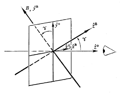
FIG. 1.: The line of sight, the plane of sky, and the direction of magnetic field. Axes $\;y^{o}\;$ and $\;z^{B}\;$ are chosen to belong to the plane defined by the line of sight and magnetic line.
 

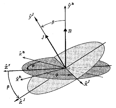
FIG. 2.: Relative positions of the coordinate systems associated with the magnetic line and with the angular momentum. The latter system is obtained from the former through a rotation about axis $\;y^{B}\;$, by angle $\;\phi\;$, and a subsequent rotation about axis $\;x^{J}\;$, by angle $\;\beta\;$.

grains, but obeys some statistical distribution determined by a particular physical setting. The above formula for $\;R\;$ was obtained in assumption of principal rotation (when the alignment of the principal axis with the angular momentum is promptly enforced), valid for suprathermally rotating grains (Lazarian & Efroimsky 1999). In the thermal case, when angle $\;\theta\;$ between the angular momentum and the major-inertia axis is nonzero, the Rayleigh factor would look more complicated:

$$R\;=\;{\Big{\langle}}\;\;\frac{3}{2}\;\left(\cos^{2}\beta\;-\;\frac{1}{3}\right)\;\;\;\frac{3}{2}\;\left(\cos^{2}\theta\;-\;\frac{1}{3}\right)\;\;{\Big{\rangle}}\;\;\;\;\;.$$ (25)

Returning to (24), we would point out the evident fact that, in the absence of alignment, the ensemble average of $\;\cos^{2}\beta\;$ is equivelent to averaging simply over the solid angle. It entails: $\;\langle\cos^{2}\beta\rangle\;=\;1/3\;$. This nullifies the R factor and makes the radiation unpolarised: $\;C_{x}^{o}\;=\;C_{y}^{o}\;$.

V Calculation of the Rayleigh reduction factor in the case when the Cross-Section Mechanism is dominant

The basic idea of the cross-section orientational process (pioneered by Lazarian 1995d, 1995e) comes from the fact that the average time between two sequent crossovers is proportional to a typical lifetime of an active site (“Purcell rocket”). Each such site is eventually “poisoned” through the evergoing accretion of atoms brought by the interstellar wind. Emergence of new active sites leads to cross-overs. Henceforth, the higher the accretion rate, the shorter the average lifetime of a typical Purcell rocket. Now, since the atoms adsorbed by the surface get delivered through the gas bombardment, one may state that the said lifetime is proportional to the rate of gas-grain collisions. The latter rate, in its turn, is proportional to the gas-grain effective cross-section, i.e., to the averaged (over the period of precession about the magnetic line) cross section of a granule, as seen by an observer looking along the line of gas flow. To summarise: the average time between two sequent crossovers is proportional to an active-site’s lifetime, the latter being proportional to the rate of gas-grain collisions, which in its turn is proportional to the effective cross section of the precessing granule in the flow. All in all, the dust particle will spend longer times in rotational states of smaller effective cross section. The cross-section mechanism is essential for the both cases of rapid and slow flows.

This line of reasoning, developed by Lazarian, brings into play several time scales. One is the period $\;t_{rot}\;$ of grain spin about its own rotation axis. The other is the wobble period $\;t_{wobble}\;$, i.e., the period of precession of the angular velocity $\;\bf\Omega\;$ and major-inertia axis $\;Z\;$ about the angular momentum $\;\bf J\;$. Third is the period $\,T\,$ of precession of $\;\bf J\;$ about the magnetic field $\;\bf B\;$. The fourth one is the mean time $\;\tau\;$ between subsequent flip-overs of the granule.

Suprathermal rotation is swift: time $\;t_{rot}\;$ is much shorter than the other time scales involved. Time $\;t_{wobble}\;$ is irrelevant in the suprathermal case, because in this case we neglect the wobble: as explained in Section I, the grain’s magnetic moment, the angular-velocity vector, and the maxumum-inertia axis are all aligned along the angular momentum, and they all precess about $\;\bf B\;$, always remaining parallel to one another. The rate of this precession about $\;\bf B\;$ is slower than the granule’s rotation, but still rapid enough: as mentioned in Section I, the precession period $\,T\,$ is much shorter than a typical interval $\;\tau\;$ between cross-overs. A cross-over of a spinning particle can happen for one (or both) of the two reasons: (1) spin damping through collisions with gas atoms, and (2) grain resurfacing that alters positions of active cites. Without going into detailed dynamics, let us assume that on the average a cross-over takes place after the granule experiences $\;N\;$ collisions. Suppose, this amount of collisions is achieved during time $\;\tau\;$:

$$N\;=\;\int_{0}^{\tau}\;n\;u\;{\big{\langle}}S{\big{\rangle}}_{\eta}\;dt$$ (26)

$n\,$ being the density of atoms, $\,u\,$ being the speed of gas flow, and $\,{\big{\langle}}S{\big{\rangle}}_{\eta}\,$ being the cross-section of the gas-grain interaction, averaged over the grain’s (principal) rotation about $\,\bf J\;$:

$${\big{\langle}}S{\big{\rangle}}_{\eta}\;=\;\frac{1}{2\pi}\;\int^{2\pi}_{0}\;S(\Phi,\;\beta,\phi,\;\eta)\;d\eta\;\;,$$ (27)

the angles $\;\Phi\;$, $\;\beta\;$, $\;\phi\;$, and $\;\eta\;$ being as on Figures 2 - 3. Even after this averaging, $\;{\big{\langle}}S{\big{\rangle}}\;$ remains time-dependent, because of the precession of $\;\bf J\;$ about $\;\bf B\;$. For times $\;\tau\;$ much longer than the precession period $\;T\;$,

$$N\;=\;\frac{\tau}{T}\;\int_{0}^{T}\;n\;u\;{\big{\langle}}S{\big{\rangle}}_{\eta}\;dt\;\;,$$ (28)

whence

$$\tau\;=\;\frac{N}{n\,u\,(1/T)\,{\int_{0}^{T}}\,{\big{\langle}}S{\big{\rangle}}_{\eta}\;dt}$$ (29)

It can be also re-written as

$$\tau\;=\;\frac{N}{n\,u\,(1/2\pi)\,\int_{0}^{2\pi}\,{\big{\langle}}S{\big{\rangle}}_{\eta}\;d\phi}\;=\;\frac{N}{n\;u\;(1/2\pi)\;\langle\;\langle S\rangle_{\eta}\rangle_{\phi}}\;\;,$$ (30)

$\,\phi\;$ being the angle as on Fig.2: during the precession period it changes from zero to $\;2\pi\;$. The usefulness of the latter expression becomes evident if one recalls that the probability to find a granule in a certain spin state is proportional to the time it stays there. After averaging over the rotation about $\;\bf J\;$, and after a further averaging over the precession, the so averaged spin state depends upon two agruments: the precession-cone half-angle $\;\beta\;$, and the angle $\;\Phi\;$ between the magnetic line and gas drift (see Fig.3). Thence, what the above formula gives us is the (not yet normalised) distribution of the (doubly averaged) spin states over $\;\beta\;$ (angle $\;\Phi\;$ being fixed and playing the role of parameter). What then remains is simply to normalise, i.e., to divide $\;\tau\;$ by its integrand over the solid angle. Thus we come to distribution

$$p_{\mbox{}}(\beta)\;=\;\frac{1}{C}\;\frac{1}{\langle\;\langle S\rangle_{\eta}\rangle_{\phi}}$$ (31)

with the normalisation constant equal to

$$C\;=\;\int_{0}^{2\pi}\;d\beta\;\sin\beta\;\frac{1}{\langle\;\langle S\rangle_{\eta}\rangle_{\phi}}\;\;$$ (32)

and the average defined as

$$\langle\;\langle S\rangle_{\eta}\rangle_{\phi}\;=\;\int_{0}^{2\pi}d\phi\;\int_{0}^{2\pi}d\eta\;\;S$$ (33)

This distribution being on our hands, the Rayleigh reduction factor is straightforward:

$$R\;=\;\;\frac{3}{2}\;\left({\Big{\langle}}\cos^{2}\beta{\Big{\rangle}}\;-\;\frac{1}{3}\right)\;=\;\frac{3}{2}\;\left(\int_{0}^{2\pi}\;d\beta\;\sin\beta\;\,p_{\mbox{}}(\beta)\;\,\cos^{2}\beta\;-\;\frac{1}{3}\right)\;$$ (34)

This is where the physics ends and mathematics begins.

VI The distribution of $\;\beta\;$ for triaxial-ellipsoid-shaped granules

In this section we shall compute the distribution $\;p_{\mbox{}}(\beta)\;$ which will, in fact, be a function of several arguments. One is, naturally, $\;\beta\;$ itself. Another will be the angle $\;\Psi\;$ between the magnetic line and the gas flow. Above that, $\;p_{\mbox{}}\;$ will depend upon the geometry of grain (in assumption that all particles in the cloud are alike).

To make the section readable, we shall move most part of the calculations to the Appendix. Remarkably, these calculations include not just exercises in geometry but also elements of the variational calculus, a heavy-duty tool seldom required in astrophysics.

We shall model the cosmic-dust particle with an ellipsoid of semiaxes $\;a\,\geq\,b\,\geq\,c\;$. Three coordinate systems will be employed. Frame $\;(X,\,Y\,Z)\;$ will be associated with semiaxes $\;a,\,b,\,c\;$, correspondingly. As we know from Section I, in the suprathermal case the major-inertia axis and the angular velocity are aligned with the angular momentum $\;\bf J\;$. So vector $\;\bf J\;$ is pointing along $\;Z\;$. Another frame, $\;(x_{B}\,,\;y_{B}\,,\;z_{B})\,$ will be associated with the magnetic field $\;\bf B\;$, axis $\;y_{B}\;$ pointing along $\;\bf B\;\,$ (Fig.2). The direction of gas flow will be denoted by unit vector $\;\bf f\;$ with components $\;(X_{f},\,Y_{f},\,Z_{f})\;$ in the body frame. The angle between $\;\bf f\;$ and axis $\;Z\;$ will be called $\;\alpha\;\,$ (Fig.3). The third coordinate system needed, $\;(x_{J}\,,\;y_{J}\,,\;z_{J})\,$

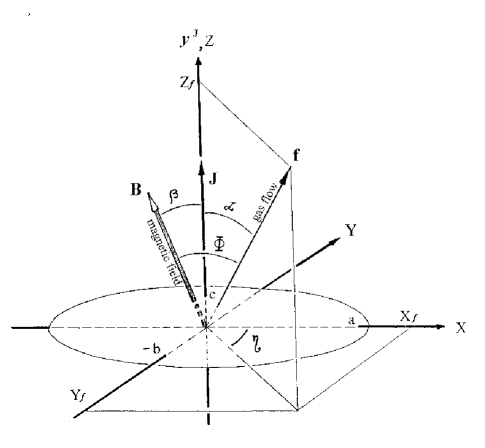
FIG. 3.: Relative orientation of the gas flow (depicted by vector $\;\bf f\;$), the
              ellipsoid’s principal axes, and its angular momentum $\;\bf J\;$. In the
              principal rotation state the major-inertia axis $\;Z\;$ of the body
              (which is its shortest dimension) is aligned with $\;\bf J\;$.

will be associated with the angular-momentum vector so that $\;y_{J}\;$ will be parallel to $\;\bf J\;$ and, therefore, to $\;Z\;$. Then axes $\;x_{J}\;$ and $\;z_{J}\;$ will belong to plane $\;(X,\,Y)\;$. One is free to parametrise the rapid rotation of the granule about its major-inertia axis $\;Z\;$ by angle $\;\eta\;$ between the least-inertia axis $\;X\;$ and the gas flow projection on the plane $\;(X,\,Y)\;$. The suprathermal spin about $\;\bf J\;$ is a much faster process than the precession of $\;\bf J\;$ about the magnetic line. Therefore, while averaging over $\;\eta\;$, one may assume the orientation of $\;\bf J\;$ being unaltered. This means that during several rotations of the granule (about $\;\bf J\;$) the angle $\;\alpha\;$ between $\;\bf J\;$ and the gas flow may be assumed unchanged. We shall also need angle $\;\Phi\;$ between the gas flow and the magnetic field, and angle $\;\beta\;$ between the magnetic field and the angular momentum. Finally, we shall parametrise the precession of $\;\bf J\;$ about $\;\bf B\;$ by angle $\;\phi\;\,$ (Fig.2). This angle is constituted by axis $\;z_{B}\;$ and axis $\;z^{\prime}\;$ (which is the projection of $\;\bf J\;$ on the plane perpendicular to $\;\bf B\;$). Without loss of generality, one can direct axis $\;x_{B}\;$ along the gas-flow projection on the plane perpendicular to $\;\bf B\;$.

As evident from Fig. 4, angles $\;\alpha\;$, $\;\beta\;$, $\;\Phi\;$ and $\;\phi\;$ are not all independent. They obey the (proven in Appendix B) relation:

$$\cos\alpha\;=\;\cos\Phi\;\cos\beta\;+\;\sin\Phi\;\sin\beta\;\sin\phi\;\;.$$ (35)

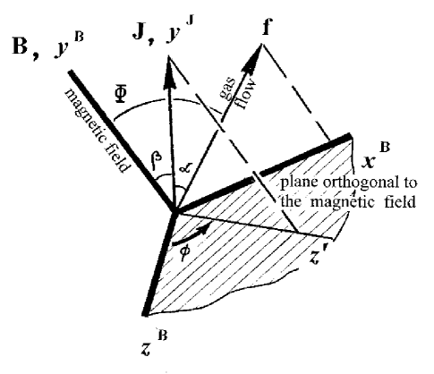
FIG. 4.: Axis $\;y^{B}\;$ is chosen to point along the magnetic line. Axis $\;x^{B}\;$ is chosen to
              point along the projection of the flow on the plane orthogonal to magnetic
              field $\;\bf B\;$. Auxiliary axis $\;z^{\prime}\;$ points along the projection of the angular mo-
              mentum $\;\bf J\;$ on the said plane.

The gas flow speeding by the ellipsoid defines an elliptic curve bounding area $\;\Sigma\;$ hatched on Fig. 5 and depicted by a thick solid line on Fig. 6. Evidently,

$$\Sigma\;=\;\pi\;|{\mbox{\boldmath$\rho$}}_{min}\;\times\;{\mbox{\boldmath$\rho$}}_{max}|\;=\;\pi\;{\rho}_{min}\;{\rho}_{max}\;\;\;,$$ (36)

${\mbox{\boldmath$\rho$}}_{min}\;$ and $\;{\mbox{\boldmath$\rho$}}_{max}\;$ being the semiaxes of hatched ellipse. Projection of $\;\Sigma\;$ on the plane orthogonal to the gas flow will give us the cross section $\;S\;$ of the granule as seen by the observer looking at it along the line of wind. As shown in Appendix B,

$$S\;=\;\pi\;\,\mid n_{x}\;\cos\eta\;\sin\alpha\;+\;n_{y}\;\sin\eta\;\sin\alpha\;+\;n_{z}\;\cos\alpha\,\mid\;\;\;,$$ (37)

where the body-frame components of the auxiliary vector $\bf n\equiv{\mbox{\boldmath$\rho$}}_{min}\times{\mbox{\boldmath$\rho$}}_{max}$ are expressed by

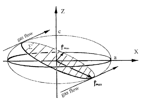
FIG. 5.: Gas flow passing by a granule is tangential to its surface in certain points.
              Altogether such points constitute an ellipse whose interior is hatched. Its
              semiaxes are vectors $\;\mbox{\boldmath$\rho$}_{min}\;$ and $\;\mbox{\boldmath$\rho$}_{max}\;$.

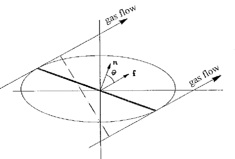
FIG. 6.: A granule in the gas flow. The thick solid line denotes cross section $\;\Sigma\;$ (the
              one that is hatched on Fig. 5).   The dashed line is the cross section $\;S\;$ of
              the granule relative to the flow. Unit vectors normal to these cross sections,
              $\bf n\;$ and $\;\bf f\;$, are separated by angle $\;\theta\;$.

$$n_{x}\;=\;(\rho_{min})_{y}\;(\rho_{max})_{z}\;-\;(\rho_{min})_{z}\;(\rho_{max})_{y}\;\;$$ (38)

and its cyclic transpositions. The components of $\;\mbox{\boldmath$\rho$}_{min}\;$ and $\;\mbox{\boldmath$\rho$}_{max}\;$ depend upon the lengths $\;a\;$, $\;b\;$, $\;c\;$ of the semiaxes, and upon their orientation relative to the gas flow, i.e., upon angles $\;\eta\;$ and $\;\alpha\;$. Angle $\;\alpha\;$, in its turn, depends upon $\;\beta\;$, $\;\Phi\;$ and $\;\phi\;$. All this will, eventually, enable us to express $\;S\;$ via $\;a\;$, $\;b\;$, $\;c\;$, $\;\beta\;$, $\;\Phi\;$, $\;\phi\;$ and $\;\eta\;$. After that we shall average over $\;\eta\;$ (i.e., over the principal rotation about $\;\bf J\;$) and over $\;\phi\;$ (i.e., over the precession of $\;\bf J\;$ about $\;\bf B\;$). It will give us the distribution (31) over $\;\beta\;$, baring dependence also upon $\;a\;$, $\;b\;$, $\;c\;$ and $\;\Phi\;$ as parameters.

Calculation of the components of vector $\;\bf n\;$ is presented in Appendix C. Plugging of these in (37) entails the following expression for the cross section of the grain placed in the flow:

$$S\,=\,\frac{\pi}{4}\,\mu_{1}\,\mu_{2}\,\mid\sin^{2}\alpha\,\cos\alpha\,\sin\eta\,\cos\eta\mid\,\left[\frac{1}{\left(b^{2}\,-\,\lambda_{2}\right)\,\left(c^{2}\,-\,\lambda_{1}\right)}\,-\,\frac{1}{\left(c^{2}\,-\,\lambda_{2}\right)\,\left(b^{2}\,-\,\lambda_{1}\right)}\right.\;\;\;$$ (39)

$$\;+\;\frac{1}{\left(c^{2}\,-\,\lambda_{2}\right)\,\left(a^{2}\,-\,\lambda_{1}\right)}\;-\;\frac{1}{\left(a^{2}\,-\,\lambda_{2}\right)\,\left(c^{2}\,-\,\lambda_{1}\right)}\;\;\;$$ (40)

$$\;\;\;\;\;\;\;\;\;\;\;\;\;\;\;\;\;\;\;\;\left.\;+\;\frac{1}{\left(a^{2}\,-\,\lambda_{2}\right)\,\left(b^{2}\,-\,\lambda_{1}\right)}\;-\;\frac{1}{\left(b^{2}\,-\,\lambda_{2}\right)\,\left(a^{2}\,-\,\lambda_{1}\right)}\;\right]$$ (41)

where

$$\mu_{1}\;=\;2\;\left(\left(\frac{\sin\alpha\;\cos\eta}{a\;\left(a^{2}\,-\,\lambda_{1}\right)}\right)^{2}\;+\;\left(\frac{\sin\alpha\;\sin\eta}{b\;\left(b^{2}\,-\,\lambda_{1}\right)}\right)^{2}\;+\;\left(\frac{\cos\alpha}{c\;\left(c^{2}\,-\,\lambda_{1}\right)}\right)^{2}\right)^{-1/2}\;\;,\;\;\;\;$$ (42)

$$\mu_{2}\;=\;2\;\left(\left(\frac{\sin\alpha\;\cos\eta}{a\;\left(a^{2}\,-\,\lambda_{2}\right)}\right)^{2}\;+\;\left(\frac{\sin\alpha\;\sin\eta}{b\;\left(b^{2}\,-\,\lambda_{2}\right)}\right)^{2}\;+\;\left(\frac{\cos\alpha}{c\;\left(c^{2}\,-\,\lambda_{2}\right)}\right)^{2}\right)^{-1/2}\;\;\;,$$ (43)

$$\lambda_{1,2}\;=\;\frac{-\;Q\;\pm\;\sqrt{Q^{2}\;-\;4\;P\;R}}{2\;P}\;\;\;,$$ (44)

$$P\;=\;\left(\frac{\sin\alpha\;\cos\eta}{a}\right)^{2}\;+\;\left(\frac{\sin\alpha\;\sin\eta}{b}\right)^{2}\;+\;\left(\frac{\cos\alpha}{c}\right)^{2}\;\;,\;\;\;\;$$ (45)

$$Q=-\left[\left(\frac{\sin\alpha\;\cos\eta}{a}\right)^{2}\left(b^{2}\,+\,c^{2}\right)\,+\,\left(\frac{\sin\alpha\;\sin\eta}{b}\right)^{2}\left(c^{2}\,+\,a^{2}\right)\,+\,\left(\frac{\cos\alpha}{c}\right)^{2}\left(a^{2}\;+\;b^{2}\right)\right]$$ (46)

$$R\;=\;\left(\frac{\sin\alpha\;\cos\eta}{a}\right)^{2}\;b^{2}\;c^{2}\;+\;\left(\frac{\sin\alpha\;\sin\eta}{b}\right)^{2}\;c^{2}\;a^{2}\;+\;\left(\frac{\cos\alpha}{c}\right)^{2}\;a^{2}\;b^{2}\;\;\;.$$ (47)

What remains is to average $\;S\;$ over $\;\eta\;$ and $\;\phi\;$ (using formula (35)), and to plug the inverse of $\;\langle\;\langle S\rangle_{\eta}\rangle_{\phi}\;$ in the expression $\;(\ref{5.6})-(\ref{5.8})\;$ for the distribution $\;p(\beta)\;$. The latter will give us, through (34), the Rayleigh reduction factor as a function of the granule dimensions $\;a,\,b,\,c\;$, and of the angle $\;\Phi\;$ between the magnetic field and the gas drift.

This work can be performed only numerically, and must be carried out with a great care. The difficulty emerges from the fact that the denominators of the terms in square brackets in the above expression (40) for $\;S\;$ vanish at certain values of the angles and at certain values of $\;a,\,b,\,c\;$. Fortunately, this is fully compensated by the multipliers $\;\mu_{1}\,\mu_{2}\,|\sin^{2}\alpha\,\cos\alpha\,\sin\eta\,\cos\eta\,|\;$ (which is most natural, for the area of a shadow cast by a smooth granule cannot have singularities). Still, when it comes to numerics, the mentioned issue demands much attention.

VII Results and their physical interpretation.

The results of computation are presented on Figures 7 - 9. As expected, the diagrammes on all three pictures show the symmetry that corresponds to the invariance under inversion of the magnetic field direction. For another easy check-up, we see that on all the diagrammes the Rayleigh reduction factor vanishes in the limit of spherical grains.

We see that the cross-section Lazarian alignment is intensive for oblate granules (Fig. 7), and approaches its maximum in the limit of “flat flake” shape. The alignment is maximal when the flow is paraller (or antiparallel) to the magnetic line, or is perpendicular thereto. Between these extremes, the alignement goes through zero. To explain this, let us consider the simple case of flate flake, and recall that the granule, roughly speaking, “wants” to minimise its (averaged over rotation and precession) cross-section as “seen” by the flow. When the flow is parallel (or antiparallel) to the magnetic line about which the grain precesses, the average cross section is minimal if the flake has its precession-cone half-angle

FIG. 7.: The Rayleigh reduction factor R as a function of the angle $\;\Phi\;$ between
          the magnetic field and the gas flow. The case of oblate symmetrical granules:
          the solid line corresponds to the semiaxes ratio $\;1\;:\;1\;:\;1/10\;\;$ (flat “flakes”),
          the circle line corresponds to $\;1:1:1/3\;,\;\;\;$ the dashed line corresponds to $\;1:1:1/2\;,$
          the star line corresponds to $\;1:1:2/3\;,\;\;\;$ the dash-dot line corresponds to $\;1:1:0.9\;$.

$\;\beta\;$ close to $\;\pi/2\;$ (and its square cosine close to nil). The $R$ factor will be negative. When the drift is orthogonal to the magnetic field, the flake “prefers” to minimise its average cross-section by rotating at $\;\beta\;$ close to zero (with its squared cosine close to unity). The $R$ factor will be positive. Therefore, $R$ passes through zero when the angle takes some intermediate value, that may be different for different ratios of semiaxes. Contrary to the expectations, though, this value, $\;\Phi_{0}^{{oblate}}\;$, bares no dependence on the semiaxes’ ratio.

FIG. 8.: The Rayleigh reduction factor R as a function of the angle $\;\Phi\;$ between
          the magnetic field and the gas flow. The case of prolate symmetrical granules:
          the solid line corresponds to the semiaxes ratio $\;1\;:\;1/10\;:\;1/10\;$ (elongated “rods”),
          the circle line corresponds to $\;1:1/3:1/3\;,\;\;\;$ the dashed line corresponds to $\;1:1/2:1/2\;$,
          the star line corresponds to $\;1:2/3:2/3\;,\;\;\;$ the dash-dot line corresponds to $\;1:0.9:0.9\;$.

As evident from Fig.8, the effect is much weaker in the case of prolate grains. The diagrammes are similar to those of oblate case, and the physical interpretation is the same as above. Just as in the case of oblate geometry, the $R$ factor goes through zero at some value of $\;\Phi\;$, that may depend on the semiaxes’ ratio. Remarkably, in this case, too, such a dependence is absent, and all the curves cross the horizontal axis in the same point $\;\Phi_{0}^{{prolate}}\;$.

Moreover, the angles $\;\Phi_{0}^{{prolate}}\;$ seems to coincide with $\;\Phi_{0}^{{oblate}}\;$ and (within the limits imposed by the calculation error) equals $\;\it{arccos}\,(1/\sqrt{3})\;$. Such miraculous coincidence must reflect some physical circumstances that are not evident at the first glance. A straightforward

FIG. 9.: The Rayleigh reduction factor R as a function of the angle $\;\Phi\;$ between
          the magnetic field and the gas flow. The case of triaxial asymmetrical granules:
          the solid line corresponds to the semiaxes ratio $\;1\;:\;0.9\;:\;0.2\;$;
          the circle line corresponds to $\;1:0.7:0.2\;;\;\;\;$ the dashed line corresponds to $\;1:0.5:0.2\;$;
          the star line corresponds to $\;1:0.3:0.2\;;\;\;\;$ the dash-dot line corresponds to $\;1:0.2:0.2\;$.

analytic proof of this “coincidence”, even in the simplest, oblate case, is unavailable.

The third picture, Fig. 9, accounts for the general case of a triaxial body, never addressed in the literature hitherto. Since the triaxial case is somewhat in-between the oblate and prolate cases, it is not surprising that the diagrammes have similar form. What $\bf{is}$ surprising, is that, once again, all the curves seem to pass zero in the same point, $\;\Phi_{o}\;=\;\it{arccos}\,(1/\sqrt{3})\;$ (and, for symmetry reasons, in $\;\Phi_{o}\;=\;\pi\;-\;\it{arccos}\,(1/\sqrt{3})\;$).

Interestingly, the Gold alignment of thermal dust fails at the same values of $\;\Phi\;$ (Dolginov & Mytrofanov 1976).

This maddening coincidence makes us suppose that this special value, $\;\Phi_{o}\;=\;\it{arccos}\,(1/\sqrt{3})\;$, is completely shape-invariant and is independent from the suprathermality degree. So here comes “the $\it{arccos}\,(1/\sqrt{3})-$hypothesis”: No mechanical alignment of arbitrarily-shaped (not necessarily ellipsoidal) thermal or suprathermal grains takes place, when the magnetic line and the gas drift make angle $\;\,\it{arccos}\,(1/\sqrt{3})\;\,$ or $\;\,\pi\,-\,\it{arccos}\,(1/\sqrt{3})$.

VIII Conclusions

In the article thus far, we have investigated the cross-section mechanism of suparthermal-grain alignment in a supersonic interstellar gas stream. While the preceding efforts had been aimed at the cases of oblate and prolate ellipsoidal grains, in the current paper we studied the case of triaxial ellipsoid. We provided a comprehensive semianalytical-seminumerical treatment that reveals the dependence of the alignment measure (Rayleigh reduction factor $R$) upon the semiaxes’ ratios and upon the angle $\Phi$ between the magnetic line and gas drift. We provided a qualitative physical explanation of some of the obtained results.

However, the most intriguing result poses a puzzle and still lacks a simple physical explanation. This is the remarkable shape-independence of the critical value of $\Phi$, at which $R$ vanishes and the cross-section mechanism fails. For all studied shapes (prolate, oblate, and triaxial with various ratios of semiaxes), this critical value is $\;\Phi_{o}\;=\;\it{arccos}\,(1/\sqrt{3})\;$. We hypothesise that this special nature of the said value of $\Phi$ is shape-independent.

A Relations between the observer-frame and body-frame extinction cross sections

Our goal is to compute the extinction cross-sections $\;C^{o}_{\it x}\;$ and $\;C^{o}_{\it y}\;$ for the two linear polarisations orthogonal to one another and to the line of sight, $\;z_{o}$. These, so-called “observer-frame” cross-sections should be expressed through extinction cross-sections $\;C_{X}\;$, $\;C_{Y}\;$, $\;C_{Z}\;$ appropriate to polarisations along the principal axes $\;X,\,Y,\,Z\;$ of the granule (with $\;X\;$, $\;Y\;$, and $\;Z\;$ standing for the minimal-, middle- and maximal-inertia axes, accordingly).

As an intermediate step, let us first calculate the intensities $\;{E^{o}_{\it x}}^{\;2}\;$ and $\;{E^{o}_{\it y}}^{\;2}\;$ appropriate to the linear polarisations, $\;x_{o}\;$ and $\;y_{o}\;$. These observer-frame intensities should be expressed through the body-frame intensities $\;E_{X}^{2}\;$, $\;E_{Y}^{2}\;$, $\;E_{Z}^{2}\;$ appropriate to polarisations along the principal axes. To that end, one has to perform a sequence of coordinate transformations.

The first step is to express $\;E^{o}_{\it x}\;$ and $\;E^{o}_{\it y}\;$ through the components $\;E^{B}_{\it{x,y,z}}\;$ of $\;\bf E\,$ in the coordinate system associated with the magnetic line. In the observer’s frame, axis $\;z_{o}\;$ points toward the telescope, while $\;y_{o}\;$ may be chosen to belong to the plane defined by $\;z_{o}\;$ and $\;\bf B\;$. Then the magnetic line will lay in the $\;(y_{o}z_{o})\,$ plane. A coordinate system associated with the magnetic field (Fig.1) may be defined with $\;y_{B}\;$ pointing along $\;\bf B\;$, and with the $\,x\,$ axis remaining untouched: $\;x_{B}\;=\;x_{o}\,$. The angle between $\;\bf B\;$ and $\;y_{o}\;$ (equal to that between $\;z_{B}\;$ and $\;z_{o}\;$) will be called $\;\gamma\;$. Hence,

$$E^{o}_{\it x}\;=\;E^{B}_{\it x}\;\;\;,\;\;\;\;\;\;E^{o}_{\it y}\;=\;E^{B}_{\it y}\;\cos\gamma\;+\;E^{B}_{\it z}\;\sin\gamma\;\;.$$ (A1)

The next transformation is from $\;(x_{B}\,,\;y_{B}\,,\;z_{B})\,$ to $\;(x_{J}\,,\;y_{J}\,,\;z_{J})\,$, the latter frame being affiliated to the (precessing about $\,\bf B\,$) angular momentum $\,\bf J\,$ of the grain. We choose $\;y_{J}\,$ to point along $\,\bf J\,$, at the angular separation $\;\beta\;$ from $\;y_{B}\;\,$ (Fig.2). Vector $\,\bf J\,$ describes, about $\,\bf B\,$, a precession cone of half-angle $\;\beta\;$; and so does $\;y_{J}\,$ about $\;y_{B}\,$. An instantaneous position of the rotating frame $\;(x_{J}\,,\;y_{J}\,,\;z_{J})\,$, with respect to the inertial one, $\;(x_{B}\,,\;y_{B}\,,\;z_{B})\,$, is determined by angle $\;\phi\;$. We see that a transition from $\;(x_{B}\,,\;y_{B}\,,\;z_{B})\,$ is two-step: first, we must revolve the basis about the $\;y_{B}$ axis by $\;\phi\;$. This will map axes $\;x_{B}\,$ and $\;z_{B}\,$ onto axes $\;x_{J}\,$ and $\;z^{\prime}\,$, accordingly. Then we rotate the basis about $\;x_{J}\,$ by angle $\;\beta\;$. In the course of a precession cycle of $\;\bf J\;$ about $\;\bf B\;$, angle $\;\beta\;$ remains unaltered, while $\;\phi\;$ describes the full circle. The relations between the unit vectors are straightforward:

$$\hat{{\bf z}}^{\prime}\;=\;\hat{{\bf z}}^{B}\;\cos\phi\;-\;\hat{{\bf x}}^{B}\;\sin\phi$$ (A2)

$$\hat{{\bf z}}^{J}\;=\;\hat{{\bf z}}^{\prime}\;\cos\beta-\hat{{\bf y}}^{B}\;\sin\beta\;=\;\hat{{\bf z}}^{B}\;\cos\phi\;\cos\beta\;-\;\hat{{\bf x}}^{B}\;\sin\phi\;\cos\beta\;-\;\hat{{\bf y}}^{B}\;\sin\beta$$ (A3)

$$\hat{{\bf y}}^{J}\;=\;\hat{{\bf y}}^{B}\;\cos\beta\;+\;\hat{{\bf z}}^{\prime}\;\sin\beta\;=\;\hat{{\bf y}}^{B}\;\cos\beta\;+\;\hat{{\bf z}}^{B}\;\cos\phi\;\sin\beta\;-\;\hat{{\bf x}}^{B}\;\sin\phi\;\sin\beta$$ (A4)

$$\hat{{\bf x}}^{J}\;=\;\hat{{\bf x}}^{B}\;\cos\phi\;+\;\hat{{\bf z}}^{B}\;\sin\phi\;\;\;.\;\;$$ (A5)

Plugging thereof into the right-hand side of the trivial identity $\;E^{B}_{\it x}\,\hat{{\bf{x}}}^{B}\,+\,E^{B}_{\it y}\,\hat{{\bf{y}}}^{B}\,+\,E^{B}_{\it z}\,\hat{{\bf{z}}}^{B}\,=\,{\bf E}\,=\,E^{J}_{\it x}\,\hat{{\bf{x}}}^{J}\,+\,E^{J}_{\it y}\,\hat{{\bf{y}}}^{J}\,+\,E^{J}_{\it z}\,\hat{{\bf{z}}}^{J}\;$ yields:

$$\;\;\;\;\;\;\;\;\;\;\;\;\;\;\;\;\;\;\;\;\;\;\;\;\;\;\;\;E^{B}_{\it x}\,=\;E^{J}_{\it x}\,\cos\phi\;-\;E^{J}_{\it y}\;\sin\phi\;\sin\beta\;-\;E^{J}_{\it z}\,\sin\phi\;\cos\beta$$ (A6)

$$\;\;\;\;\;\;\;\;\;\;\;\;\;\;\;\;\;\;\;E^{B}_{\it y}\,=\;\;\;\;\;\;\;\;\;\;\;\;\;\;\;\;\;\;\;\;E^{J}_{\it y}\;\cos\beta\;\;\;\;\;\;\;\;\;\;-\;E^{J}_{\it z}\,\sin\beta$$ (A7)

$$\;\;\;\;\;\;\;\;\;\;\;\;\;\;\;\;\;\;\;\;\;\;\;\;\;\;\;E^{B}_{\it z}\,=\;E^{J}_{\it x}\,\sin\phi\;+\;E^{J}_{\it y}\;\cos\phi\;\sin\beta\;+\;E^{J}_{\it z}\,\cos\phi\;\cos\beta$$ (A8)

Lastly, we take into account the position of the grain itself, relative to coordinates $\;(x^{J},\,y^{J},\,z^{J})\;$. As explained in the Introduction (footnote 1), it is legitimate in the suprathermal case to assume that the major-inertia axis $\,Z\,$ of the particle is aligned with the angular momentum, i.e., with axis $\,y^{J}\;$ (for details see Lazarian & Efroimsky 1999). Rotation of the granule is, thus, assumed principal and may be parametrised by the angle $\;\psi\;$ between the least-inertia axis $\;X\;$ and $\;z^{J}\;$ (this angle is equal to that between the middle-inertia axis $\;Y\;$ and $\;x^{J}\;$). This gives:

$$E^{J}_{\it x}\;=\;-\;E_{X}\;\sin\psi\;+\;E_{Y}\;\cos\psi$$ (A9)

$$\;E^{J}_{\it y}\;=\;\;\;\;E_{Z}\;\;\;\;\;\;\;\;\;\;\;\;\;\;\;\;\;\;\;\;\;\;\;\;\;\;\;\;\;\;$$ (A10)

$$\;E^{J}_{\it z}\;=\;\;\;E_{X}\;\cos\psi\;+\;E_{Y}\;\sin\psi\;\;.$$ (A11)

Combination of all the afore presented transformations results in:

$$E^{o}_{\it x}\;=\;E^{B}_{\it x}\;=\;E^{J}_{\it x}\,\cos\phi\;-\;E^{J}_{\it y}\;\sin\phi\;\sin\beta\;-\;E^{J}_{\it z}\,\sin\phi\;\cos\beta\;=$$ (A12)

$$=\;E_{X}\;(\,-\;\sin\psi\;\cos\phi\;-\;\cos\psi\;\sin\phi\;\cos\beta)\;\;\;\;\;\;\;\;\;\;\;\;\;\;\;\;\;\;\;\;\;\;\;\;\;\;$$ (A13)

$$+\;E_{Y}\;(\cos\psi\;\cos\phi\;-\;\sin\psi\;\sin\phi\;\cos\beta)\;-\;E_{Z}\;\sin\phi\;\sin\beta\;\;\;\,$$ (A14)

and

$$E^{o}_{\it y}\,=\,E^{B}_{\it y}\,\cos\gamma\,+\,E^{B}_{\it z}\,\sin\gamma\,=\;\;\;\;\;\;\;\;\;\;\;\;\;\;\;\;\;\;\;\;\;\;\;\;\;\;\;\;\;\;\;\;\;\;\;\;\;\;\;\;\;\;\;\;\;\;\;\;\;\;\;\;\;\;\;\;\;\;\;\;\;\;\;\;\;\;\;\;\;\;\;\;\;\;\;$$ (A15)

$$\left(E^{J}_{\it y}\,\cos\beta\,-\,E^{J}_{\it z}\,\sin\beta\right)\,\cos\gamma\,+\,\left(E^{J}_{\it x}\,\sin\phi\,+\,E^{J}_{\it y}\,\cos\phi\,\sin\beta\;+\;E^{J}_{\it z}\,\cos\phi\;\cos\beta\right)\,\sin\gamma\;\;\;\;\;\;$$ (A16)

$$=\,E_{X}\;(\,-\;\sin\psi\;\sin\gamma\;\sin\phi\;-\;\cos\psi\;\cos\gamma\;\sin\beta\;+\;\cos\psi\;\cos\phi\;\sin\gamma\;\cos\beta)$$ (A17)

$$+\;E_{Y}\;(\cos\psi\;\sin\gamma\;\sin\phi\;-\;\sin\psi\;\cos\gamma\;\sin\beta\;+\;\sin\psi\;\cos\phi\;\sin\gamma\;\cos\beta)\;\;\;\;\;\;$$ (A18)

$$+\;E_{Z}\;(\cos\gamma\;\cos\beta\;+\;\sin\gamma\;\cos\phi\;\sin\beta)\;\;\;,\;\;\;\;\;\;\;\;\;\;\;\;\;\;\;\;\;\;\;\;\;\;\;\;\;\;\;\;\;\;\;\;\;\;\;\;\;\;\;\;\;\;\;\;\;\;\;\;\;\;\;$$ (A19)

whence the averaged-over-the-ensemble intensities read:

$$\langle{E_{x}^{o}}^{2}\rangle\;=\;\frac{1}{4}\;E_{X}^{2}\;\left(1\;+\;{\Big{\langle}}\cos^{2}\beta{\Big{\rangle}}\right)\;+\;\frac{1}{4}\;E_{Y}^{2}\;\left(1\;+\;{\Big{\langle}}\cos^{2}\beta{\Big{\rangle}}\right)\;+\;\frac{1}{2}\;E_{Z}^{2}\;{\Big{\langle}}\sin^{2}\beta{\Big{\rangle}}\;=$$ (A20)

(A21)

$$\frac{1}{3}\;\left(E_{X}^{2}\;+\;E_{Y}^{2}\;+\;E_{Z}^{2}\right)\;+\;\frac{1}{3}\;\left[\frac{1}{2}\;\left(E_{X}^{2}\;+\;E_{Y}^{2}\right)\;-\;E_{Z}^{2}\right]\;\frac{3}{2}\;\left({\Big{\langle}}\cos^{2}\beta{\Big{\rangle}}\;-\;\frac{1}{3}\right)$$ (A22)

$$=\;\frac{1}{3}\;\left(E_{X}^{2}\;+\;E_{Y}^{2}\;+\;E_{Z}^{2}\right)\;+\;\frac{1}{3}\;\left[\frac{1}{2}\;\left(E_{X}^{2}\;+\;E_{Y}^{2}\right)\;-\;E_{Z}^{2}\right]\;R$$ (A23)

and

$${\Big{\langle}}{E_{y}^{o}}^{2}{\Big{\rangle}}\;=\;E_{X}^{2}\;\left(\frac{1}{4}\;\sin^{2}\gamma\;+\;\frac{1}{2}\;\cos^{2}\gamma\;\,{\Big{\langle}}\sin^{2}\beta{\Big{\rangle}}\;+\;\frac{1}{4}\;\sin^{2}\gamma\;\,{\Big{\langle}}\cos^{2}\beta{\Big{\rangle}}\right)\;+$$ (A24)

$$\;\;\;\;\;\;\;\;\;\;\;E_{Y}^{2}\;\left(\frac{1}{4}\,\sin^{2}\gamma\;+\;\frac{1}{2}\,\cos^{2}\gamma\;{\Big{\langle}}\sin^{2}\beta{\Big{\rangle}}\;+\;\frac{1}{4}\,\sin^{2}\gamma\;{\Big{\langle}}\cos^{2}\beta{\Big{\rangle}}\right)\;+$$ (A25)

$$E_{Z}^{2}\;\left(\cos^{2}\gamma\;\,{\Big{\langle}}\cos^{2}\beta{\Big{\rangle}}\;+\;\frac{1}{2}\;\sin^{2}\gamma\;\,{\Big{\langle}}\sin^{2}\beta{\Big{\rangle}}\right)\;=\;\;\;\;\;\;\;\;\;\,$$ (A26)

$$\frac{1}{3}\;\left(E_{X}^{2}\;+\;E_{Y}^{2}\;+\;E_{Z}^{2}\right)\;+\;\left(\frac{1}{3}\;-\;\cos^{2}\gamma\right)\;\left[\frac{1}{2}\;\left(E_{X}^{2}\;+\;E_{Y}^{2}\right)\;-\;E_{Z}^{2}\right]\;\frac{3}{2}\;\left(\langle\cos^{2}\beta\rangle\;-\;\frac{1}{3}\right)$$ (A27)

$$=\;\frac{1}{3}\;\left(E_{X}^{2}\;+\;E_{Y}^{2}\;+\;E_{Z}^{2}\right)\;+\;\left(\frac{1}{3}\;-\;\cos^{2}\gamma\right)\;\left[\frac{1}{2}\;\left(E_{X}^{2}\;+\;E_{Y}^{2}\right)\;-\;E_{Z}^{2}\right]\;R$$ (A28)

Following the established tradition, we single out the so-called Rayleigh reduction factor

$$R\;=\;\frac{3}{2}\;\left(\;{\Big{\langle}}\;\cos^{2}\beta\;{\Big{\rangle}}\;-\;\frac{1}{3}\;\right)\;\;.$$ (A29)

In (A23) - (A28) averaging over $\;\psi\;$ and $\;\phi\;$ implies simply $\;(2\pi)^{-2}\,\int_{0}^{2\pi}d\psi\;\int_{0}^{2\pi}d\phi\;$, while the averaging over $\;\beta\;$ remains so far unspecified; the appropriate distribution depends upon the physics of gas-grain interaction and is calculated in Section V.

Now, that we have expressed the observable intensities $\;\langle{E_{x}^{o}}^{2}\rangle\;$ and $\;\langle{E_{y}^{o}}^{2}\rangle\;$ via those appropriate to polarisations along the body axes, we can write down similar expressions interconnecting the extinction cross sections. Since the extinction is merely attenuation of power from the incident beam, the contributions to cross-section from the body-axes’ directions will be proportional to the mean shares of power appropriate to these three axes:

$$C^{o}_{x}\;=\;\frac{C_{X}\;+\;C_{Y}\;+\;C_{Z}}{3}\;+\;\frac{1}{3}\;\left[\;\frac{1}{2}\;\left(C_{X}\;+\;C_{Y}\right)\;-\;C_{Z}\;\right]\;R$$ (A30)

and

$$C^{o}_{y}\;=\;\frac{C_{X}\;+\;C_{Y}\;+\;C_{Z}}{3}\;+\;\left(\frac{1}{3}\;-\;\cos^{2}\gamma\right)\;\left[\;\frac{1}{2}\;\left(C_{X}\;+\;C_{Y}\right)\;-\;C_{Z}\;\right]\;R$$ (A31)

wherefrom

$$C^{o}_{x}\;-\;C^{o}_{y}\;=\;\left[\;\frac{1}{2}\;\left(C_{X}\;+\;C_{Y}\right)\;-\;C_{Z}\;\right]\;R\;\cos^{2}\gamma\;\;\;.$$ (A32)

B Ellipsoidal granule placed in a magnetic field and gas flow. Several useful formulae.

Here we prove several formulae used in the text. Let us begin with relations for the angle $\;\alpha\;$ between the gas-flow direction $\;\bf f\;$ and the maximum-inertia axis $\;Z\;$ of the dust particle (Fig. 4). Dot product of the appropriate unit vectors

$$\hat{\bf y}_{J}\;=\;{\hat{\bf y}}_{B}\;\cos\beta\;+\;\hat{\bf z}_{B}\;\sin\beta\;\cos\phi\;+\;\hat{\bf x}_{B}\;\sin\beta\;\sin\phi$$ (B1)

and

$${\bf f}\;=\;{\hat{\bf y}}_{B}\;\cos\Phi\;+\;\hat{\bf z}_{B}\;\sin\Phi$$ (B2)

leads to formula:

$$\cos\alpha\;=\;\cos\Phi\;\cos\beta\;+\;\sin\Phi\;\sin\beta\;\sin\phi\;\;.$$ (B3)

Another important relation is evident from Fig. 3:

$$\cos\alpha\;=\;\frac{Z_{f}}{\sqrt{X_{f}^{2}\;+\;Y_{f}^{2}\;+\;Z_{f}^{2}}}\;\;.$$ (B4)

On Fig.3, the projection of $\;\it\bf f\;$ on $\;(X,\,Y)\;$ will make an angle $\,\eta\,$ with axis $\,X\,$, such that

$$\cos\eta\;\sin\alpha\;=\;\frac{X_{f}}{\sqrt{X_{f}^{2}\;+\;Y_{f}^{2}\;+\;Z_{f}^{2}}}\;\;\;,\;\;\;\;\;\;\;\;\sin\eta\;\sin\alpha\;=\;\frac{Y_{f}}{\sqrt{X_{f}^{2}\;+\;Y_{f}^{2}\;+\;Z_{f}^{2}}}$$ (B5)

Formulae (B4) and (B5) will enable us to calculate the grain’s cross section relative to the wind. The lines of gas flow, which are tangential to the ellipsoid surface, touch this surface in points that altogether constitute a curve. It is the ellipse hatched on Fig. 5. Its area is:

$$\Sigma\;=\;\pi\;|{\mbox{\boldmath$\rho$}}_{min}\;\times\;{\mbox{\boldmath$\rho$}}_{max}|\;=\;\pi\;{\rho}_{min}\;{\rho}_{max}$$ (B6)

${\mbox{\boldmath$\rho$}}_{min}\;$ and $\;{\mbox{\boldmath$\rho$}}_{max}\;$ being its semiaxes. Projection of $\;\Sigma\;$ toward the plane perpendicular to the gas flow is the cross section $\;S\;$ of the granule, as seen by the observer looking at it along the line of wind (Fig. 6). In other words, $\;S\;$ is the “shadow” that the granule casts. Evidently,

$$S\;=\;|\cos\theta|\;\,\Sigma$$ (B7)

$\theta\;$ being the angle between the vector $\;\bf f\;$ of the gas flow and vector

$${\bf n}\;\equiv\;{\mbox{\boldmath$\rho$}}_{min}\;\times\;{\mbox{\boldmath$\rho$}}_{max}$$ (B8)

orthogonal to the hatched ellipse. As follows from (B4 - B5),

$$|\cos\theta|\;=\;\frac{{\bf n\;\cdot f}}{|\bf n|\;|\bf f|}\;=\;\frac{|n_{x}\;X_{f}\;+\;n_{y}\;Y_{f}\;+\;n_{z}\;Z_{f}|}{\left(\Sigma/\pi\right)\;\sqrt{X_{f}^{2}\,+\,Y_{f}^{2}\,+\,Z_{f}^{2}}}\;=$$ (B9)

(B10)

$$\frac{\pi}{\Sigma}\;\;|n_{x}\;\cos\eta\;\sin\alpha\;+\;n_{y}\;\sin\eta\;\sin\alpha\;+\;n_{z}\;\cos\alpha\,|\;.$$ (B11)

Combining the above with (B7), we arrive to:

$$S\;=\;\pi\;\,|n_{x}\;\cos\eta\;\sin\alpha\;+\;n_{y}\;\sin\eta\;\sin\alpha\;+\;n_{z}\;\cos\alpha\,|\;\;.$$ (B12)

C Cross Section of a granule arbitrarily oriented in the gas stream

Every point $\;(X,\,Y,\,Z)\;$ belonging to the surface of the ellipsoidal grain obeys equation

$$g(X,\,Y,\,Z;\,a,\,b,\,c)\;\equiv\;\frac{X^{2}}{a^{2}}\;+\;\frac{Y^{2}}{b^{2}}\;+\;\frac{Z^{2}}{c^{2}}\;=\;1\;\;.$$ (C1)

The points, that constitute the boundary of the hatched figure $\,\Sigma\,$ on Fig.5, obey (C1), along with one more relation. That second one is the condition of flow being tangential to the surface in these points. Stated alternatively: a normal to the ellipsoid in point $\;(X,\,Y,\,Z)\;$ is given by vector $\;(X/a^{2},\,Y/b^{2},\,Z/c^{2})\;$, and the flow must be orthogonal to this normal:

$$h(X,\,Y,\,Z;\,X_{f},\,Y_{f},\,Z_{f})\;\equiv\;\frac{X\;X_{f}}{a^{2}}\;+\;\frac{Y\;Y_{f}}{b^{2}}\;+\;\frac{Z\;Z_{f}}{c^{2}}\;=\;0\;\;.$$ (C2)

To find vectors $\;{\mbox{\boldmath$\rho$}}_{min}\;$ and $\;{\mbox{\boldmath$\rho$}}_{max}\;$ pointing from the centre to the closest and the farthest points of the ellipse $\;\Sigma\;$, one has to employ the variational method:

$$\frac{\partial}{\partial X,\,Y,\,Z}\;\left({\it l}^{2}\;-\;\lambda\;g\;-\;\mu\;h\right)\;=\;0$$ (C3)

where $\;{\it l}^{2}\;\equiv\;X^{2}\;+\;Y^{2}\;+\;Z^{2}\;$, and $\;\lambda,\,\mu\;$ are Lagrange multipliers. The latter equation gives us the values of $\;X,\,Y,\,Z\;$ appropriate to the extremal distances from the origin, in assumption that constraints (C1) and (C2) hold. Three equations (C3), for $\;X,\,Y\,$ and $\,Z\;$, yield:

$$X\;=\;\frac{\mu\;X_{f}}{2\;\left(a^{2}\;-\;\lambda\right)}\;\;,\;\;\;Y\;=\;\frac{\mu\;Y_{f}}{2\;\left(b^{2}\;-\;\lambda\right)}\;\;,\;\;\;Z\;=\;\frac{\mu\;Z_{f}}{2\;\left(c^{2}\;-\;\lambda\right)}$$ (C4)

for the extremal points where vectors $\;\pm\,{\mbox{\boldmath$\rho$}}_{min}\;$ and $\;\pm\,{\mbox{\boldmath$\rho$}}_{max}\;$ end. To find the values of $\;\lambda\;$, plug (C4) in (C2):

$$h\;=\;\mu\;\frac{X^{2}_{f}}{2\;a^{2}\;\left(a^{2}\;-\;\lambda\right)}\;+\;\mu\;\frac{Y^{2}_{f}}{2\;b^{2}\;\left(b^{2}\;-\;\lambda\right)}\;+\;\mu\;\frac{Z^{2}_{f}}{2\;c^{2}\;\left(c^{2}\;-\;\lambda\right)}\;=\;0\;\;.$$ (C5)

This entails:

$$\lambda_{1,2}\;=\;\frac{-\;Q\;\pm\;\sqrt{Q^{2}\;-\;4\;P\;R}}{2\;P}$$ (C6)

where

$$P\;\equiv\;\left(\frac{X_{f}}{a}\right)^{2}\;+\;\left(\frac{Y_{f}}{b}\right)^{2}\;+\;\left(\frac{Z_{f}}{c}\right)^{2}\;\;,\;\;\;\;$$ (C7)

$$Q\;\equiv\;-\;\left[\;\left(\frac{X_{f}}{a}\right)^{2}\;\left(b^{2}\;+\;c^{2}\right)\;+\;\left(\frac{Y_{f}}{b}\right)^{2}\;\left(c^{2}\;+\;a^{2}\right)\;+\;\left(\frac{Z_{f}}{c}\right)^{2}\;\left(a^{2}\;+\;b^{2}\right)\;\right]\;\;,\;\;\;\;$$ (C8)

$$R\;\equiv\;\left(\frac{X_{f}}{a}\right)^{2}\;b^{2}\;c^{2}\;+\;\left(\frac{Y_{f}}{b}\right)^{2}\;c^{2}\;a^{2}\;+\;\left(\frac{Z_{f}}{c}\right)^{2}\;a^{2}\;b^{2}\;\;\;.$$ (C9)

Substitution of (C4) in (C1) will lead to the expression for $\;\mu\;$:

$$\mu^{2}\;=\;4\;\left(\left(\frac{X_{f}}{a\;\left(a^{2}\,-\,\lambda\right)}\right)^{2}\;+\;\left(\frac{Y_{f}}{b\;\left(b^{2}\,-\,\lambda\right)}\right)^{2}\;+\;\left(\frac{Z_{f}}{c\;\left(c^{2}\,-\,\lambda\right)}\right)^{2}\;\right)^{-1}$$ (C10)

Since we have two acceptable values for $\;\lambda\;$, we shall obtain four different values for $\;\mu\;$:

$$\mu_{1}\;=\;2\;\left(\left(\frac{X_{f}}{a\;\left(a^{2}\,-\,\lambda_{1}\right)}\right)^{2}\;+\;\left(\frac{Y_{f}}{b\;\left(b^{2}\,-\,\lambda_{1}\right)}\right)^{2}\;+\;\left(\frac{Z_{f}}{c\;\left(c^{2}\,-\,\lambda_{1}\right)}\right)^{2}\right)^{-1/2}\;\;,\;\;\;\;$$ (C11)

$$\mu_{2}\;=\;2\;\left(\left(\frac{X_{f}}{a\;\left(a^{2}\,-\,\lambda_{2}\right)}\right)^{2}\;+\;\left(\frac{Y_{f}}{b\;\left(b^{2}\,-\,\lambda_{2}\right)}\right)^{2}\;+\;\left(\frac{Z_{f}}{c\;\left(c^{2}\,-\,\lambda_{2}\right)}\right)^{2}\right)^{-1/2}\;\;,$$ (C12)

and $\;\mu_{3}\;=\;-\;\mu_{1}\;,\;\;\mu_{4}\;=\;-\;\mu_{2}\;$. Simply from looking at how $\;\lambda\;$ and $\;\mu\;$ enter expressions (C4) for extremal-point coordinates, we see that a change of sign of $\;\mu\;$ (with $\;\lambda\;$ fixed) corresponds merely to a switch from $\;{\mbox{\boldmath$\rho$}}_{min}\;$ (or $\;{\mbox{\boldmath$\rho$}}_{max}\;$) to $\;-\,{\mbox{\boldmath$\rho$}}_{min}\;$ (or $\;-\,{\mbox{\boldmath$\rho$}}_{max}\;$, appropriately). Since it is irrelevant, for our purposes, which of the two opposite farmost from the origin points to call $\;{\mbox{\boldmath$\rho$}}_{max}\;$ and which to call $\;-\,{\mbox{\boldmath$\rho$}}_{max}\;$ (and, similarly, which of the two closemost to the origin points to call $\;{\mbox{\boldmath$\rho$}}_{min}\;$ and which to call $\;-\,{\mbox{\boldmath$\rho$}}_{max}\;$), we shall take the positive values of $\;\mu\;$ only. As a result, a substitution of $\;\lambda_{1}\;$ and $\;\mu_{1}\;$ in (C4) will give us the coordinates of one of the two farthest, from the centre, points of the boundary of the hatched ellipse $\;\Sigma\;$. Similarly, plugging of $\;\lambda_{2}\;$ and $\;\mu_{2}\;$ will provide us with the coordinates of one of the two closest points. The chosen farthest and closest points will have coordinates $\;(\rho_{max})_{x,y,z}\;$ and $\;(\rho_{min})_{x,y,z}\;\,$, appropriately:

$$(\rho_{max})_{x}\;=\;\frac{\mu_{1}\;X_{f}}{2\;\left(a^{2}\,-\,\lambda_{1}\right)}\;\;,\;\;\;(\rho_{max})_{y}\;=\;\frac{\mu_{1}\;Y_{f}}{2\;\left(b^{2}\,-\,\lambda_{1}\right)}\;\;,\;\;\;(\rho_{max})_{z}\;=\;\frac{\mu_{1}\;Z_{f}}{2\;\left(c^{2}\,-\,\lambda_{1}\right)}\;\;,$$ (C13)

and

$$(\rho_{min})_{x}\;=\;\frac{\mu_{2}\;X_{f}}{2\;\left(a^{2}\,-\,\lambda_{2}\right)}\;\;,\;\;\;(\rho_{min})_{y}\;=\;\frac{\mu_{2}\;Y_{f}}{2\;\left(b^{2}\,-\,\lambda_{2}\right)}\;\;,\;\;\;(\rho_{min})_{z}\;=\;\frac{\mu_{2}\;Z_{f}}{2\;\left(c^{2}\,-\,\lambda_{2}\right)}\;\;.$$ (C14)

Further substitution of these expressions in (38) and in its cyclic transpositions will lead to:

$$n_{x}\;X_{f}\;=\;X_{f}\;Y_{f}\;Z_{f}\;\frac{\mu_{1}\;\mu_{2}}{4}\;\left[\frac{1}{\left(b^{2}\,-\,\lambda_{2}\right)\,\left(c^{2}\,-\,\lambda_{1}\right)}\;-\;\frac{1}{\left(c^{2}\,-\,\lambda_{2}\right)\,\left(b^{2}\,-\,\lambda_{1}\right)}\right]$$ (C15)

$$n_{y}\;Y_{f}\;=\;X_{f}\;Y_{f}\;Z_{f}\;\frac{\mu_{1}\;\mu_{2}}{4}\;\left[\frac{1}{\left(c^{2}\,-\,\lambda_{2}\right)\,\left(a^{2}\,-\,\lambda_{1}\right)}\;-\;\frac{1}{\left(a^{2}\,-\,\lambda_{2}\right)\,\left(c^{2}\,-\,\lambda_{1}\right)}\right]$$ (C16)

$$n_{z}\;Z_{f}\;=\;X_{f}\;Y_{f}\;Z_{f}\;\frac{\mu_{1}\;\mu_{2}}{4}\;\left[\frac{1}{\left(a^{2}\,-\,\lambda_{2}\right)\,\left(b^{2}\,-\,\lambda_{1}\right)}\;-\;\frac{1}{\left(b^{2}\,-\,\lambda_{2}\right)\,\left(a^{2}\,-\,\lambda_{1}\right)}\right]$$ (C17)

Thence the cross section $\;S\;$ of the grain, relative to the gas-flow direction, will read:

$$S\;=\;\frac{\pi}{4}\;\mu_{1}\;\mu_{2}\;{|X_{f}\;Y_{f}\;Z_{f}|}\;\left[\frac{1}{\left(b^{2}\,-\,\lambda_{2}\right)\,\left(c^{2}\,-\,\lambda_{1}\right)}\;-\;\frac{1}{\left(c^{2}\,-\,\lambda_{2}\right)\,\left(b^{2}\,-\,\lambda_{1}\right)}\right.\;\;\;$$ (C18)

$$\;+\;\frac{1}{\left(c^{2}\,-\,\lambda_{2}\right)\,\left(a^{2}\,-\,\lambda_{1}\right)}\;-\;\frac{1}{\left(a^{2}\,-\,\lambda_{2}\right)\,\left(c^{2}\,-\,\lambda_{1}\right)}\;\;\;$$ (C19)

$$\;\;\;\;\;\;\;\;\;\;\;\;\;\;\;\;\;\;\;\;\left.\;+\;\frac{1}{\left(a^{2}\,-\,\lambda_{2}\right)\,\left(b^{2}\,-\,\lambda_{1}\right)}\;-\;\frac{1}{\left(b^{2}\,-\,\lambda_{2}\right)\,\left(a^{2}\,-\,\lambda_{1}\right)}\;\right]$$ (C20)

where $\;\lambda_{1,2}\;$ and $\;\mu_{1,2}\;$ are functions of $\;(X_{f},\,Y_{f},\,Z_{f})\;$, the latter being functions of angles $\;\eta\;$ and $\;\alpha\;$ (while $\;\alpha\;$ is, in its turn, depends upon $\;\beta\;$, $\;\Phi\;$, and $\;\phi\;$). All in all, the “shadow” area $\;S\;$ turns to be a function of angles $\;\beta\;$, $\;\Phi\;$, $\;\eta\;$, and $\;\phi\;$.

REFERENCES

- [1] Alpar, A., and H. Ögelman. 1987. Neutron Star Precession and the Dynamics of the Superfluid Interior. Astronomy and Astrophysics, 185, p. 196
- [2] Bisnovatyi-Kogan, G. S., and P. Kahabka. 1993. Period Variations and Phase Residuals in Freely Precessing Stars. Astronomy and Astrophysics, 267, p. L43
- [3] Dolginov, A. Z., and I. G.Mitrofanov. 1976. Orientation of Cosmic-Dust Grains. Astrophysics and Space Science, 43, p. 291
- [4] Draine, B.T., and H.-M. Lee. 1985. Optical properties of interstellar graphite and silicate grains. Astrophys. J., 285, p. 89
- [5] Draine, B.T., and J. C. Weingartner. 1996. Radiative Torques on Interstellar Grains. I. Superthermal Spin-up. Astrophys. J., 470, p. 551
- [6] Draine, B.T., and J. C. Weingartner. 1997. Radiative Torques on Interstellar Grains. II. Grain Alignment. Astrophys. J., 480, p. 633
- [7] Davis, J., and J. L. Greenstein. 1951. The polarisation of starlight by aligned dust grains. Astrophys. J., 114, p. 206
- [8] Efroimsky, Michael. 2000. Precession of a Freely Rotating Rigid Body. Inelastic Dissipation in the Vicinity of Poles. Journal of Mathematical Physics, 41, p. 1854
- [9] Efroimsky, Michael, & A.Lazarian 2000. Inelastic Dissipation in Wobbling Asteroids and Comets. Monthly Notices of the Royal Astronomical Society, 311, p. 269
- [10] Efroimsky, Michael. 2001. Relaxation of Wobbling Asteroids and Comets. Theoretical Problems. Perspectives of Experimental Observation. Planetary & Space Science, 49, p. 937
- [11] Efroimsky, Michael. 2002. Euler, Jacobi, and Missions to Comets and Asteroids. Advances in Space Research, to be published.
- [12] Gold, T. 1952. The alignment of galactic dust. Monthly Notices of the Royal Astronomical Society, 112, p. 215
- [13] Greenberg, J.M. 1968. Interstellar Grains. In: Nebulae and Interstellar Matter, Vol. VII, pp. 221 - 364, ed. Middlehurst, B. M., and L. H. Aller. University of Chicago Press, Chicago
- [14] Hall, J.S. 1949. Observation of the Polarised Light from Stars. Science, 109, p. 166
- [15] Hildebrand, R.H. 1988. Magnetic Fields and Stardust. Quarterly Journal of the Royal Astronomical Society, 29, p. 327.
- [16] Hiltner, W.A. 1949. Polarisation of light from distant stars by interstellar medium. Astrophys. J., 109, p. 471
- [17] Jones, R.V., and L. Spitzer, Jr. 1967. Magnetic alignment of interstellar grains. Astrophys. J., 147, p. 943
- [18] Lazarian, A. 1994. Gold-Type Mechanisms of Grain Alignment. Monthly Notices of the Royal Astronomical Society, 268, p. 713
- [19] Lazarian, A. 1995a. Physics and chemistry of the Purcell alignment. Monthly Notices of the Royal Astronomical Society,274, p. 679
- [20] Lazarian, A. 1995b. Paramagnetic alignment of fractal grains. Astronomy & Astrophysics, 293, p. 859
- [21] Lazarian, A. 1995c. Davis-Greenstein Alignment of Nonspherical Grains. Astrophys. J., 453, p. 229
- [22] Lazarian, A. 1995d. Mechanical Alignment of Suprathermally Rotating Grains. Astrophys. J., 451, p. 660
- [23] Lazarian, A. 1995e. Alignment of suprathermally rotating grains. Monthly Notices of the Royal Astronomical Society, 277, p. 1235
- [24] Lazarian, A., and Michael Efroimsky. 1996. Cross-Section Alignment of Oblate Suprathermal Grains. Astrophys. J., 466, p. 274
- [25] Lazarian, A., Michael Efroimsky, and Jonathan Ozik. 1996. Mechanical Alignment of Prolate Cosmic-Dust Grains. Astrophys. J., 472, p. 240
- [26] Lazarian, A., and Michael Efroimsky. 1999. Inelastic Dissipation in a Freely Rotating Body. Application to Cosmic-Dust Alignment. Monthly Notices of the Royal Astronomical Society, 303, p. 673
- [27] Lazarian, A., and B. T. Draine. 1997. Disorientation of Suprathermally Rotating Grains and the Grain Alignment Problem. Astrophys. J., 487, p. 248
- [28] Lazarian, A., and W. G. Roberge. 1997. Barnett relaxation in thermally rotating grains. Astrophys. J., 484, p. 230
- [29] Lee, H. M., and B. T. Draine. 1985. Infrared extinction and polarisation due to partially aligned spheroidal grains: models for the dust toward the BN object. Astrophys. J., 290, p. 211
- [30] Martin, P.G. 1971. On interstellar grain alignment by a magnetic field. Monthly Notices of the Royal Astronomical Society, 153, p. 279
- [31] Martin, P.G. 1974. Interstellar polarisation from a medium with changing grain alignment. Astrophys. J., 187, p. 461
- [32] Purcell, E.M. 1979. Suprathermal Rotation of Interstellar Grains. Astrophys. J., 231, p. 404
- [33] Purcell, E.M., and L. Spitzer, Jr. 1971. Orientation of rotating grains. Astrophys. J., 167, p. 31
- [34] Roberge, W.G., T. A. DeGraff, and J.E. Flaherty. 1993. The Langevin Equation and Its Application to Grain Alignment in Molecular Clouds Astrophys. J., 418, p. 287
- [35] Roberge, W.G., and A. Lazarian. 1999. Davis-Greenstein alignment of oblate spheroidal grains. Monthly Notices of the Royal Astronomical Society, 305, p. 615
- [36] Spitzer, L., and J. W. Tukey. 1951. A theory of interstellar polarisation. Astrophys. J., 114, p. 187
- [37] Stairs, I. H., et al. 2000. Evidence for Free Precession in a Pulsar. Nature 406, p. 484
- [38] Stoner, E.C. 1934, Magnetism and Matter, Methuen Publ., London, UK
- [39] Trümper, J., P. Kahabka, H. Ögelman, W. Pietsch, and W. Voges. 1986. Astrophys. J. Letters, 300, p. L63
- [40] van de Hulst, H. C. 1957. Light Scattering by Small Particles Dover, NY
- [41] Whittet, D.C.B. 1992. Dust in the Galactic Environment. IOP Publishers, Bristol, UK.