IP Pegasi: Investigation of the accretion disk structure

We present the results of spectral investigations of the cataclysmic variable IP Peg in quiescence. Optical spectra obtained on the 6-m telescope at the Special Astrophysical Observatory (Russia), and on the 3.5-m telescope at the German-Spanish Astronomical Center (Calar Alto, Spain), have been analysed by means of Doppler tomography and Phase Modelling Technique. From this analysis we conclude that the quiescent accretion disk of IP Peg has a complex structure. There are also explicit indications of spiral shocks. The Doppler maps and the variations of the peak separation of the emission lines confirm this interpretation. We have detected that all the emission lines show a rather considerable asymmetry of their wings varying with time. The wing asymmetry shows quasi-periodic modulations with a period much shorter than the orbital one. This indicates the presence of an emission source in the binary rotating asynchronously with the binary system. We also have found that the brightness of the bright spot changes considerably during one orbital period. The spot becomes brightest at an inferior conjunction, whereas it is almost invisible when it is located on the distant half of the accretion disk. Probably, this phenomenon is due to an anisotropic radiation of the bright spot and an eclipse of the bright spot by the outer edge of the accretion disk.

1 Introduction

IP Pegasi is a well-known deeply eclipsing dwarf nova with an orbital period of 3$\aas@@fstack{h}$79 (Lipovetskij & Stephanyan Lipov:Steph (1981); Wolf et al. Wolf93 (1993)) and an outburst cycle of about 2.5 months. During high states, which last about 12 days, the system changes from V magnitude 14th during quiescence (out of eclipse) to 12 during outburst. Many times IP Peg was subject to detailed spectral investigations (Marsh & Horne marsh:horne90 (1990); Marsh marsh88 (1988); Martin et al. Martin (1989); Hessman Hessman (1989); Harlaftis et al. Harlaftis94 (1994); Wolf et al. Wolf98 (1998)) and photometric researches (Wolf et al. Wolf93 (1993); Szkody & Mateo Szkody (1986); Wood & Crawford Wood86 (1986); Wood et al. Wood89 (1989); Bobinger et al. Bobinger97 (1997)). In the last years IP Peg deserved increasing interest as spiral shocks were detected in its accretion disk during outburst (Steeghs et al. Steeghs97 (1997); Harlaftis et al. Harlaftis99 (1999)).

The question on the existence of spiral shocks in the accretion disks has a long standing history. It is closely related to angular momentum transport mechanisms in accretion disks. At present there are two approaches to this problem: According to the first one, angular momentum is transported due to the presence of turbulent or magnetic viscosity in the disk (Shakura & Sunyaev Shak:Sun (1973)). On the other hand, hydrodynamical numerical calculations have shown that tidal forces of the secondary induce spiral shock waves in the accretion disk, which may provide an efficient transfer mechanism (Sawada et al. Japan86 (1986); Matsuda et al. Japan90 (1990)). Self-similar solutions having spiral shocks, was constructed in a semi-analytic manner in two dimensions by Spruit (Spruit (1987), see also Chakrabarti Chak (1990)). It should be noted that these two mechanisms are mutually exclusive, as shock waves in the presence of viscosity will be smeared out (Bunk et al. Bunk (1990); Chakrabarti Chak (1990)). Although Steeghs et al. (1997) found indications for spiral shocks in the hot accretion disks during an outburst, the problem on the spiral structure of the quiescent accretion disks still remains unsolved.

Most theorists do not support the hypothesis of the presence of spiral shocks in the accretion disks in quiescence due to the following arguments:

Since the disk expands during outburst (Smak Smak84 (1984); Wolf et al. Wolf93 (1993)), the outer parts of the expanded disk are subject to higher gravitational attraction of the secondary, leading to the formation of spiral arms. The tidal force is a very steep function of the distance to the secondary star, hence the spiral shocks rapidly become weak at smaller disk sizes. Furthermore, the opening angle of the spirals is directly related to the temperature of the disk as it roughly propagates at sound speed. This effect was the principal reason to believe that spirals may not be present in accretion disks of cataclysmic variables, which are not hot enough. This is in principal the case in quiescent disks (Boffin Boffin01 (2001)). Steeghs & Stehle found from their calculations (Stehle99 (1999)), using the grid of the 2D hydrodynamic accretion disk, that the spiral shocks in quiescent accretion disks are so tightly wound that they leave few fingerprints in the emission lines.

At the same time, the authors of the most comprehensive 3D simulations are in principle inclined to accept the presence of spiral shocks in the relatively cold disks. So, Makita et al. (Japan00 (2000)) observed in their 3D calculations that spiral shocks are formed in an accretion disk for all specific heat ratios. In addition, they claim that in cool disks, when comparing 3D calculations with 2D ones, spiral arms are less tightly wound in the outer region of the disk. In connection with this, it is important to add that in 3D disks, there is a vertical resonance that can lie within the disk. This resonance causes a local thickening of the disk and generates waves that propagate radially. The first wavelength of this wave is longer than that of the usual 2D waves by a factor of about $(R/H)^{1/3}$ (Lubow Lubow (1981)). The wavelength does increase with the level of non-linearity (Yuan & Cassen Yuan:Cassen (1994)). The non-linear effects can modify significantly the appearance of the spiral pattern: a longer wavelength produces a less tightly wound spiral pattern. Obviously the observations matches more closely a 3D disk, and the 2D approximation can poorly explain the observations. [Indeed, the two-dimensional disk simulations demonstrate that the spiral pattern resembles the observations only for unreally high temperatures (see, for example, Godon et al. Godon (1998)).] And at last, the calculations of Bisikalo et al. (1998a ; 1998b , see also Kuznetsov et al. Kuznetsov (2001)) only yield the one-armed spiral shock in the quiescent accretion disk. In the place where the second arm should form, the stream from $L_{1}$ dominates and presumably prevents the formation of the second arm of the tidally induced spiral shock.

Thus, as stated above, the existence of the spiral shocks in the quiescent accretion disk has not been established convincingly. Their observational detection would be very important because spiral arms are indeed very efficient in transporting angular momentum into the outer part of the disk. If existing at all, spiral shocks would be much more difficult to detect than the strong shocks in the hot accretion disk during outburst. Nevertheless, first steps towards an observational confirmation have been started. So, studying the structure of the accretion disk of U Gem in quiescence we have detected sinusoidal variations ($\sin 2\varphi$) of the double peak separations of the hydrogen emission lines and of their shape (Borisov & Neustroev bor:neus2 (1999)). These variations are the signature of an m=2 mode in the disk. This mode can be excited by the tidal forcing. We showed that such orbital behavior of the emission lines can be reproduced by means of a simple model of the accretion disk with two symmetrically located spiral shocks (Neustroev & Borisov Neus:Bor (1998)). Recently we have found, by means of Doppler tomography, new confirmation for spiral shocks in the quiescent accretion disk of U Gem (Neustroev et al. Neus2002 (2002)). Further investigations in this area are strongly recommended.

The main goal of the present paper was the investigation of the accretion disk structure of IP Peg in order to locate the line emitting sites during quiescence. Special attention was payed to the search for evidences for a spiral structure of the accretion disk. Section 2 of this paper describes the observations and data reduction procedures, while Sect. 3 describes an average spectrum and emission lines variations. Section 4 presents the analysis of the optical spectra by means of Doppler tomography and Phase Modelling Technique. The results are discussed in Sect. 5 and summarized in Sect. 6.

Figure 1: The mean normalized spectra of IP Peg, based on first dataset.

2 Observations

The spectra presented here were obtained during two observing runs. The first spectroscopic observations of IP Peg were performed on July 13, 1993 using a 1000-channel television scanner mounted on the SP-124 spectrograph at the Nasmyth-1 focus of the 6-m telescope of the Special Astrophysical Observatory. A total of 40 spectra were taken in the wavelength range 3600-5500 Å with a dispersion of 1.9 Å channel^-1. The weather conditions were not very favorable, with a seeing of around 3 arcseconds. Individual exposure times were 300 s, and the intervals between them did not exceed 30 s. The total duration of the observations was 3.8 hours. Note that we observed IP Peg in its quiescent state. We reduced these spectroscopic data by using the procedure described by Knyazev (Knyazev (1994)).

A second dataset was obtained during an observing campaign in August 06-09 1994 at the 3.5-m telescope at the German-Spanish Astronomical Center, Calar Alto, Spain. From the trailed spectra, which were phase-folded into 100 phase bins and which have a spectral resolution of 1.3 Å, we extracted the H$\alpha$, H$\beta$ and H$\gamma$ lines. Due to technical difficulties we could only obtain 50% phase coverage of H$\alpha$. Data acquisition and reduction methods used are described in detail by Wolf et al. (Wolf98 (1998)).

3 Average spectrum and emission lines variations

The mean normalized spectrum of IP Peg, based on first dataset, is shown in Fig. 1. The mean spectrum for second dataset can be found in Wolf et al. (Wolf98 (1998), Fig. 2). Before averaging the single spectra were shifted according to the $K_{1}\sin(\phi)$, with $K_{1}$ = 168 km s^-1 (Wolf et al. Wolf98 (1998)). For the calculation of orbital phases the ephemeris of Wolf et al. (Wolf93 (1993)) was used:

$T_{0}(HJD)=2445615.4156+0.15820616\cdot E$,

where $T_{0}$ is the moment of mid-eclipse.

Both spectra show strong, broad hydrogen and helium emission lines. The trailed spectra of the major hydrogen lines are shown in Fig. LABEL:trailed (note that the data are displayed twice for clarity). Their double-peaked profiles are thought to be associated with the accretion disk. They are superposed by asymmetric structures produced by anisotropically radiating emission regions of the binary system. The line profiles demonstrate a puzzling behaviour the blue-shifted peak being stronger than the red-shifted peak when averaged over the orbit.

Figure 3: The degree of asymmetry of the emission line H$\beta$ folded with the orbital period (top panel: first dataset, bottom panel: second dataset). The degree of asymmetry is the ratio between the areas of violet and red peaks of the emission line. Filled circles show individual values, open circles with dotted line show data which were obtained by averaging adjacent data points. The data are plotted twice for continuity.

Figure 4: Some profiles of the H$\beta$ line which show the rather considerable asymmetry of its wings. It can be seen that from time to time on blue and red wings a hump appears.

We have measured the degree of asymmetry of each line profile, and have plotted this parameter against the orbital phase (in the following this plot is named: the S-wave graph). We have calculated the degree of asymmetry $S$ as the ratio between the areas of violet and red peaks of the emission line. Let us highlight the principal features of the resulting curves (Fig. 3). Note first that their shape obviously deviates from of a sine wave, although for an accretion disk with a single bright spot it should be nearly sinusoidal (Borisov and Neustroev bor:neus1 (1998)). In addition to this, the amplitude of this intensity variation of the blue peak exceeds by far that for the red peak. However, it can be seen that the degree of asymmetry with $S>1$ is observed only during one-half of the orbital period, whereas $S\leq 1$ is found at other times. The possible reasons for such variations of the degree of asymmetry can be an anisotropic radiation of the bright spot and/or an eclipse of the bright spot by the outer edge of the accretion disk. These assumptions will be discussed in the course of further analysis.

A closer inspection of the line profiles shows that all the emission lines exhibit a considerable asymmetry of their wings which varies with time. This effect is observed in both data sets but most notably in the first one. The visual analysis has shown that from time to time a hump appears on the blue and red wings (Fig. 4). Its shift concerning the center of the line does not exceed $\sim$1200–1400 km s^-1.

To describe the wing asymmetry WA quantitatively, we define the following quantity:

$$WA=\left\{{\begin{array}[]{*{20}c}{VR-1}&{\begin{array}[]{*{20}c}{\hskip 42.67912ptVR>1}\\ \end{array}}\\ {1-VR^{-1}}&{\begin{array}[]{*{20}c}{\hskip 42.67912ptVR<1}\\ \end{array}}\\ \end{array}}\right.$$ (1)

where

$$VR={{\sum\nolimits_{\lambda_{0}-d\lambda}^{\lambda_{0}-(d\lambda+\Delta\lambda)}{I_{\lambda}}}\mathord{\left/\,{\vphantom{{\sum\nolimits_{\lambda_{0}-d\lambda}^{\lambda_{0}-(d\lambda+\Delta\lambda)}{I_{\lambda}}}{\sum\nolimits_{\lambda_{0}+\lambda_{b}}^{\lambda_{0}+(d\lambda+\Delta\lambda)}{I_{\lambda}}}}}\right.\kern-1.2pt}{\sum\nolimits_{\lambda_{0}+d\lambda}^{\lambda_{0}+(d\lambda+\Delta\lambda)}{I_{\lambda}}}}$$

Here ${\lambda_{0}}$ is the wavelength of the center of the line, and $d{\lambda}$ defines the beginning of the wavelength interval ${\Delta\lambda}$ in which the fluxes are summed up.

To see how the wing asymmetry of the emission lines depends on time, we calculated the degree of the wing asymmetry of all H$\beta$ profiles and plotted their values against the time of observations (Fig. 5, upper left panel). In this case we have used following parameters: $d{\lambda}$ = 15 Å and ${\Delta\lambda}$ = 10 Å. It can be seen that the wing asymmetry shows quasi-periodic modulations with a period much shorter than the orbital one. This indicates the presence of an emission source rotating asynchronously with the binary system.

We looked for periods in this data sample using the Scargle (Scargle (1982)) method and tested our results using the AoV method (Schwarzenberg-Czerny Sch-Cz (1989)) and the PDM algorithm (Phase Dispersion Minimization, Stellingwerf Stellingwerf (1978)).

The calculated periodogram shows three strong peaks at 0$\aas@@fstack{h}$61, 0$\aas@@fstack{h}$33 and 1$\aas@@fstack{h}$67, the first one being little bit stronger of them (Fig. 5, lower left panel). This result was confirmed applying the AoV and PDM methods. As an example we have fitted the wing asymmetry’s data from Fig. 5 (upper left panel) by a simple sinusoid with the period of 0$\aas@@fstack{h}$61 and have plotted this curve by a dotted line in the same figure.

A detailed discussion of the line-wings‘ variations is given in Sect. 5.

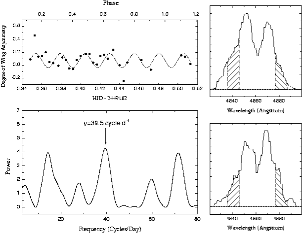
Figure 5: In the upper left panel is shown the degree of the wing asymmetry of the emission line H$\beta$ from the first dataset plotted against the time of observations. These data have been fitted by the simple sinusoid with the period 0$\aas@@fstack{h}$61 (dotted line). In the lower left panel the periodogram of the above data is shown. The periodogram shows three strong peaks at 0$\aas@@fstack{h}$61, 0$\aas@@fstack{h}$33 and 1$\aas@@fstack{h}$67, the first one is the little bit stronger of them. In the right-hand column are shown some profiles of the H$\beta$ line in which the wavelength range used for the determination of the degree of the wing asymmetry has been marked.

4 Investigation of the structure of the accretion disk

The orbital variations of the emission line profiles indicate a non-uniform structure of the accretion disk. For its study we have used the Doppler tomography and the Phase Modelling Technique.

4.1 The Doppler tomography

Doppler tomography is an indirect imaging technique which can be used to determine the velocity-space distribution of the line’s emission in close binary systems. Full details of the method are given by Marsh & Horne (marsh:horne (1988)). Doppler maps of the major emission lines were computed using the filtered backprojection algorithm described by Robinson et al. (robinson (1993)). Since we cannot assume any relation between position and velocity during eclipse we constrained our data sets by removing eclipse spectra covering the phase ranges $\varphi=0.90-0.10$.

The constructed Doppler maps of the H$\beta$, H$\gamma$ and H$\delta$ emission from the first dataset are shown in Fig. 6 (left column). Though the tomograms based on the spectra from the second dataset, were already published, we find it useful to present here again the Doppler maps of H$\alpha$, H$\beta$ and H$\gamma$ (Fig. 7, left column). The figures also show the positions of the white dwarf, the center of mass of the binary and the secondary star, and also the trajectories of free particles released from the inner Lagrangian point. Additionally, the velocity of the disk along the path of the gas stream is plotted in each Doppler map.

The tomograms show at least the two bright emitting regions superposed on the typical ring-shaped emission of the accretion disk. The bright emission region with coordinates $V_{x}\approx$ 0 $-$ -800 km s^-1 and $V_{y}\approx$ 0 $-$ 700 km s^-1 (first dataset) and V${}_{x}\approx$ -200 $-$ -800 km s^-1 and $V_{y}\approx$ 200 $-$ 600 km s^-1 (second dataset) can be unequivocally contributed to emission from the bright spot on the outer edge of the accretion disk. The second spot with coordinates $V_{x}\approx$ 700 $-$ 800 km s^-1 and $V_{y}\approx$ 50 km s^-1 (first dataset, most notable in H${\beta}$ and H${\delta}$) and $V_{x}\approx$ 200 $-$ 800 km s^-1 and $V_{y}\approx$ -900 $-$ 300 km s^-1 (second dataset) locate far from the region of interaction between the stream and the disk particles. The nature of this spot is analysed in the following section.

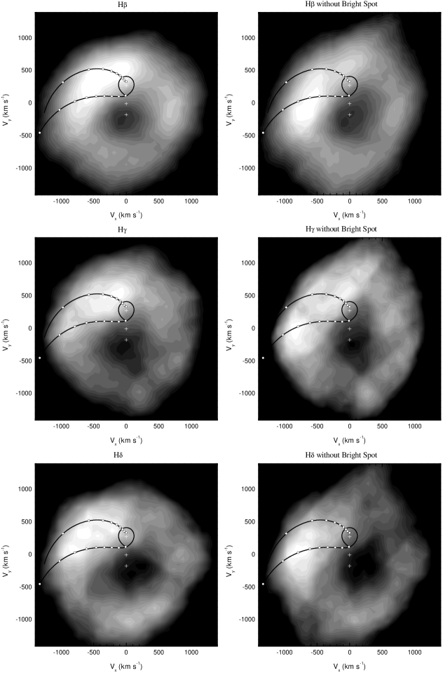
Figure 6: Doppler maps of H${\beta}$, H${\gamma}$ and H${\delta}$ emission obtained from the first dataset. Left column: Doppler maps based on all spectra. Right column: the maps based on those spectra which were obtained at minimum spot brightness (for details see text).

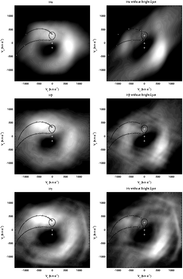
Figure 7: Doppler maps of H${\alpha}$, H${\beta}$ and H${\gamma}$ emission obtained from the second dataset. Left column: Doppler maps based on all spectra. Right column: the maps based on those spectra which were obtained at minimum spot brightness (for details see text).

4.2 The modelling

Although the Doppler tomography is a very robust technique which can analyse the structure of the accretion disk, it still has some imperfections. We shall note only one of them. This technique makes no allowance for changes in the intensity of features over an orbital cycle. Components which do vary will be handled incorrectly, and the obtained tomograms will be averaged on the period. In our recent paper (Borisov & Neustroev bor:neus1 (1998)) we have presented another technique for the investigation of the structure of the accretion disk, which is based on the modelling of the profiles of the emission lines formed in a non-uniform accretion disk. The analysis has shown that the modelling of the spectra obtained in different phases of the orbital period, allows to estimate the principal parameters of the spot, though its spatial resolution is worse. However, there is also an important advantage — the method allows to investigate the modification of the spot’s brightness with orbital phase. This cannot be done by Doppler tomography.

For an accurate calculation of the line profiles formed in the accretion disk, it is necessary to know the velocity field of the radiating gas, its temperature and density, and, first of all, to calculate the radiative transfer equations in the lines and the balance equations. Unfortunately, this complicated problem has not been solved until now and it is still not possible to reach an acceptable consistency between calculations and observations. Nevertheless, even the simplified models allow one to derive some important parameters of the accretion disk.

In our calculations we have applied a double-component model which include the flat Keplerian geometrically thin accretion disk and the bright spot whose position is constant with respect to components of the binary system (Fig. 8). We began the modelling of the line profiles with calculation of a symmetrical double-peaked profile formed in the uniform axisymmetrical disk, then we added the distorting component formed in the bright spot. To calculate the line profiles we have used the method of Horne & Marsh (Horne:Marsh (1986)), taking into account the Keplerian velocity gradient across the finite thickness of the disk.

Free parameters of our model are:

1. $R=R_{in}$/R_out is the ratio of the inner and outer radii of the disk;

2. $V$ is the velocity of the outer rim of the accretion disk;

3. $\alpha$ is an emissivity parameter (the line surface brightness of the disk is assumed to scale as R^-α);

4. $\vartheta$ is an angle between the direction from the primary to the secondary and the center of the bright spot respectively (a phase angle);

5. $\Psi$ is a spot azimuthal extent;

6. $R_{S}$ is a radial position of the spot’s center in fractions of the outer radius ($R_{out}$=1);

7. $\Delta R_{S}$ is a radial extent;

8. $L$ is a relative dimensionless luminosity of the spot, which is given by

   $\begin{array}[t]{l}L=\int\limits_{R_{S}-\Delta R_{S}/2}^{R_{S}+\Delta R_{S}/2}S\cdot B\cdot f(r)\cdot dr=\\ \\ =\frac{\pi}{180}\frac{\Psi\Delta R_{S}B}{2-\alpha}\left[\left(R_{S}+\frac{\Delta R_{S}}{2}\right)^{2-\alpha}-\left(R_{S}-\frac{\Delta R_{S}}{2}\right)^{2-\alpha}\right]\end{array}$

   where $S$ is area of the spot, and $B$ is the spot’s contrast (the spot-to-disk brightness ratio at the same distance from the white dwarf).

The results of testing have shown (Borisov and Neustroev bor:neus1 (1998)) that for a reliable estimation of the parameters it is important to keep the certain sequence of their determination. This is connected with the strong azimuth dependence of the emission line profile with variation of various spot parameters. When modelling the emission lines of IP Peg, we determined the parameters in the following order:

• The orbital-phase modulation of the degree of asymmetry of the profile is used to find the phase angle of the spot $\vartheta$;

• Spectroscopic data are then sorted according to the ”maximally effective” phases for various parameters of the spot: the azimuthal extent of the spot $\Psi$ can be best determined at azimuths -$30^{\circ}-30^{\circ}$ and $150^{\circ}-210^{\circ}$, and the radial position of the spot $R_{S}$ can be best determined at azimuths $50^{\circ}-130^{\circ}$ and -$50^{\circ}-$ -$130^{\circ}$;

• The azimuthal extent of the spot is determined, fixed, and then used in the estimation of the radial position of the spot in the accretion disk;

• The remaining profiles are modelled with values of the already determined geometrical spot parameters fixed, in order to derive the relative luminosity of the spot at various orbital phases.

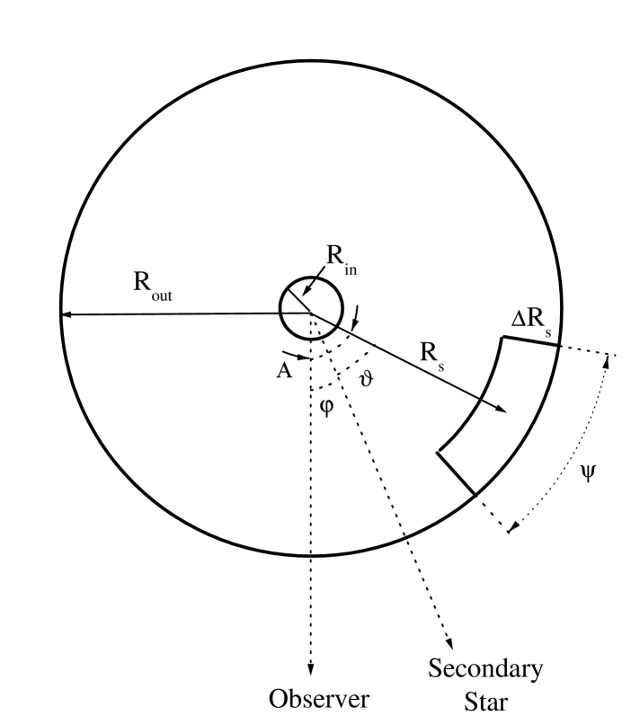
Figure 8: Accretion disk geometry for the line profile model described in the text.

Table 1: Average parameters of the accretion disk and the bright spot obtained by modelling separate spectra

Emission	Dataset	$\alpha$	$R$	$V$	$\vartheta$	$\Psi$	$\Delta R_{s}^{\ast}$	$R_{s}$	Contrast
line
H${\beta}$	First	1.67 $\pm$ 0.49	0.08 $\pm$ 0.04	570 $\pm$ 100	30	50 $\pm$ 15	0.1	0.95 $\pm$ 0.05	2.1 $\pm$ 1.5
H${\beta}$	Second	1.61 $\pm$ 0.40	0.08 $\pm$ 0.03	590 $\pm$ 106	29	49 $\pm$ 18	0.1	0.96 $\pm$ 0.05	2.0 $\pm$ 1.1
H${\gamma}$	First	2.15 $\pm$ 0.56	0.08 $\pm$ 0.03	549 $\pm$ 130	30	75 $\pm$  6	0.1	0.90 $\pm$ 0.10	3.1 $\pm$ 2.6
H${\gamma}$	Second	1.69 $\pm$ 0.47	0.08 $\pm$ 0.04	616 $\pm$ 102	26	42 $\pm$  5	0.1	0.89 $\pm$ 0.08	4.9 $\pm$ 4.9
H${\delta}$	First	1.68 $\pm$ 0.78	0.12 $\pm$ 0.06	669 $\pm$ 155	30	52 $\pm$ 16	0.1	0.88 $\pm$ 0.08	3.6 $\pm$ 3.2

$\ast$ Adopted by default.

Since the shape of the profile is virtually independent of variations in the radial extent of the spot $\Delta R_{S}$ (Borisov & Neustroev bor:neus1 (1998)), a default value for this parameter can be used in the profile computations (e.g., a typical radial extent of the bright spot). Photometric observations of the cataclysmic variables indicate that the radial extent of the spots vary from  0.02 to  0.15 (Rozyczka Rozyczka (1988)). We adopted the value $\Delta R_{S}$ = 0.1.

The necessary condition for the accurate determination of the spot parameters is the knowledge of its phase angle $\vartheta$, which possibly can be found from the analysis of the phase variations of the degree of asymmetry of the emission line (S-wave graph). We must determine $\varphi_{0}$. This phase corresponds to the moment when the radial velocity of the S–wave component is zero. Then the phase angle $\vartheta$ of the spot will be $2\pi(1-\varphi_{0})$. Examples of the application of this technique to real data are given in Neustroev (neustroev (1998)) and Borisov & Neustroev (bor:neus2 (1999)).

For the study of the accretion disk structure of IP Peg it was possible to apply this technique to all major emission lines (H$\alpha$, H$\beta$, H$\gamma$ and H$\delta$), but because of signal-to-noise limitations the discussion, following below, is mostly based on the H$\beta$ line. We have started our analysis of the spectroscopic data by determination of the phase angle $\vartheta$ of the spot, using the S-wave graph (Fig. 3). The value of $\vartheta$ has been found to be 30^∘ (H$\beta$, H$\gamma$ and H$\delta$ lines from first dataset), 29^∘ (the H$\beta$ line from second dataset) and 26^∘ (the H$\gamma$ line from second dataset) respectively.

As a result of subsequent modelling we have established all principal parameters of the accretion disk and the bright spot. Their average values are listed in Table 1. It is necessary to note that the standard deviations of all averaged parameters of the disk are considerably higher than expected on the basis of testing (Borisov & Neustroev bor:neus1 (1998)). It may be due to possible orbital variations of the observed parameters of the accretion disk.

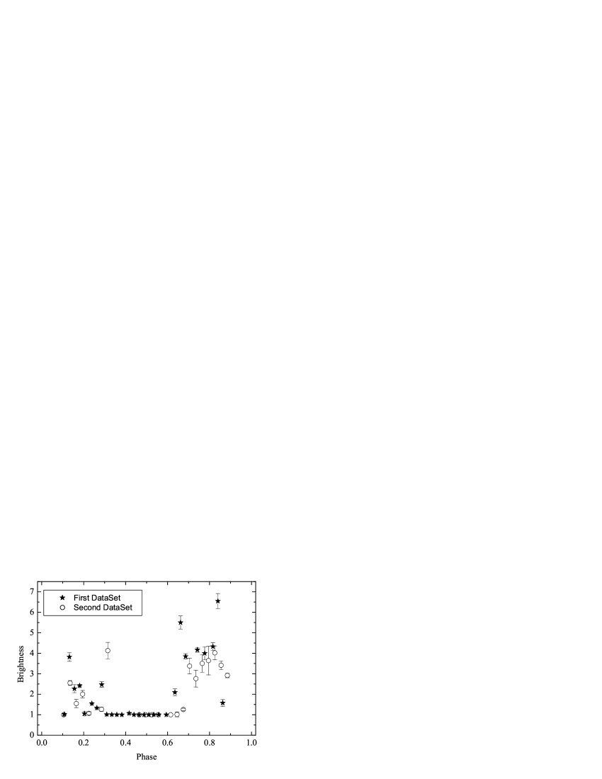
Figure 9: The dependence of the spot brightness on orbital phase, obtained from modelling of the H$\beta$ emission line. Obviously the brightness considerably oscillates, and during a significant part of the period the spot is not visible.

5 Discussion

As already noted in Sect. 4.1, our Doppler maps show two bright emitting regions (Figs. 6 and 7, left column). Now we also point out that the part of the bright region which we have interpreted as bright spot, is located near the intersection of a ring-shaped structure and the upper arc of the tomograms. It indicates the nearly Keplerian velocities of the matter in the area of the bright spot.

The modelling of the Balmer line profiles has allowed us to find the dependence of the brightness of this spot on the orbital phase (Fig. 9). The derived brightness curves of the spot for both observing sets are very similar. One can see that the brightness considerably oscillates, and during a significant part of the period ($\varphi\sim$ 0.2 to 0.6) the spot is not visible. This happens when the spot is on the distant half of the accretion disk. On the contrary, the spot becomes brightest at the moment of inferior conjunction. It is important to note that even near to the moment of inferior conjunction the brightness of the spot varies. Probably, this is connected to an anisotropic radiation of the bright spot. In consequence of it we get an asymmetric change in radiation during one orbital revolution of the system. However, the anisotropy alone cannot explain the missing emission of the bright spot during the orbital phases when the spot has turned away from the observer’s point of view. (In this case it is more correct to name ”a bright spot” as ”an invisible hot spot”.) We think this fact can additionally be explained by a self-eclipse of the bright spot owing to the large inclination of the orbital plane of IP Peg and of its accretion disk. This scenario causes an eclipse of the bright spot by an outer edge of the accretion disk followed by a drop of observable spot brightness. Thus we suggest at least two mechanisms for explanation of the observable variations of the spot brightness: an anisotropic radiation of the bright spot and an eclipse of the bright spot by the outer edge of the accretion disk. We have no possibility to discuss in this paper, which of these mechanisms is more important. It will be the subject of the separate paper.

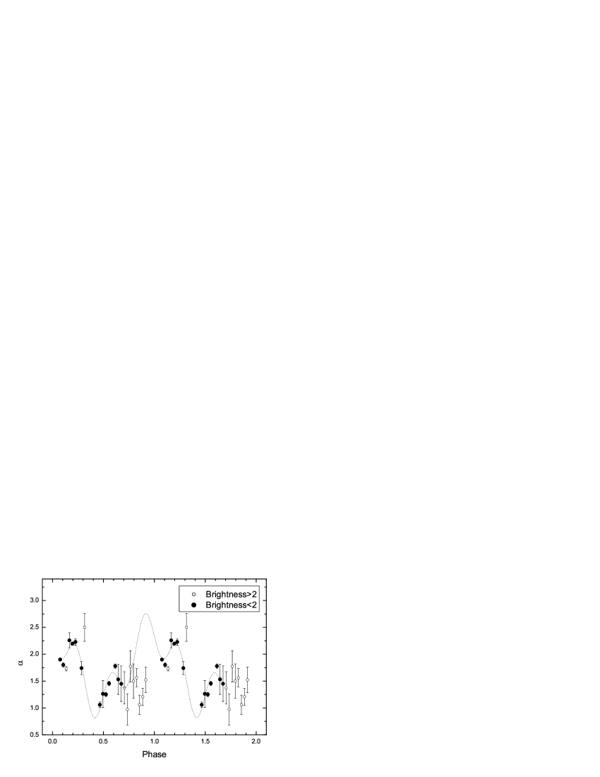
Figure 10: The dependence of the velocity of the outer edge of the accretion disk (top panel) and of the emissivity parameter $\alpha$ (bottom panel) on orbital phase, obtained on basis of modelling H$\beta$ emission line from the second dataset. Filled and open circles represent those values of parameters, which were found on spectra obtained in phases of minimum and maximum brightness of the spot respectively.

The second area of increased luminosity is located too far from the region of interaction between the stream and the disk particles. None of the theories do predict here the presence of a bright spot, which is connected with such an interaction. This area was interpreted recently by Wolf et al. (Wolf98 (1998)) as beginning of the formation of a spiral arm in the outer disk in context of the tidal force from the secondary.

The majority of the simulations predicts the presence of the spiral structure with two symmetrically located spiral shocks in the accretion disk. Exactly such a two-armed structure was detected by Steeghs et al. (Steeghs97 (1997)) in the accretion disk of IP Peg during outburst. However, the second spiral arm in our tomograms is not visible. If it does exist, it is probably hidden in the intensive emission of the bright spot. If the contribution of the bright spot from the initial profiles of the emission lines (or from the resulting Doppler maps), could be removed, it may be possible to detect the second spiral arm.

For this we have constructed the new Doppler maps using only half of the spectra obtained in phases of minimum brightness of the spot ($\varphi$ = 0.15 to 0.65) (Figs. 6 and 7, right column). Although the used profiles of the emission lines practically do not contain information about the bright spot, on the left side of the Doppler maps we can see an area of increased luminosity! However its location has changed. It was displaced downwards and has taken practically a symmetrical position concerning the second area of the increased luminosity. However, in contradiction to Steeghs et al (Steeghs97 (1997)), we cannot confidently assert that the form of both bright areas is spiral, first of all because of their low brightness. Indeed, the emissivity contrast between the proposed spirals and other parts of the disk is less than 1.3 for all emission lines. At the same time we consider that even the really spiral features in the tomograms can be caused by a different effect than the spiral shocks (see, for example, Smak Smak01 (2001); Ogilvie Ogilvie (2001)). Additional evidences for this are necessary.

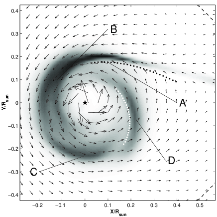
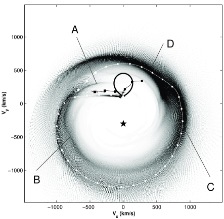
Figure 11: Left: The distribution of $\rho^{2}T^{1/2}$ over the equatorial plane in 3D calculations of Kuznetsov et al. (Kuznetsov (2001)) ($\rho$ is density, $T$ is temperature). Arrows are the velocity vectors in observer’s frame. The asterisk is the white dwarf. The white dotted line is the tidally induced spiral shock. A black dotted line is the shock wave along the edge of the stream (‘hot line’). The main emission regions are marked by A, B, C, D. Right: Synthetic Doppler map for $I\sim\rho^{2}T^{1/2}$. The secondary Roche lobe (a bold black line) and the white dwarf (an asterisk) are also shown. The white line with circles and black line with squares show gas dynamical trajectories in the velocity coordinates. The main emission regions are marked by A, B, C, D as above. Both figures are reproduced under the kind permission by O.A. Kuznetsov and D.V. Bisikalo.

Additional evidences for a spiral structure of the accretion disk of IP Peg arise from the dependence of the velocity of the outer edge of the disk on orbital phase. Earlier, studying the structure of the accretion disk of U Gem, we have detected a sinusoidal variation of the parameters of the disk (and especially the velocities V of its outer edge) of the form $\sin 2\varphi$. We interpreted this by the presence of a spiral structure (Neustroev & Borisov Neus:Bor (1998)) in the disk of U Gem. We have tried to detect similar effects in IP Peg. In Fig. 10 (top panel) the dependence of the velocity of the accretion disk on orbital phase is shown. One can see, that the amplitude of variation of V in this case is even higher than for U Gem. However, the most significant variations of velocity occur at the moment of maximum brightness of the spot. In this case we cannot unequivocally eliminate the probable influence of the bright spot on the double peak separation of the emission lines. Therefore in Fig. 10 we have selected those values of velocity V, which were found from spectra obtained in phases of minimum brightness of the spot. Such a spot distorts the line profile only marginally, therefore the velocity V is determined confidently.

Although the dependence of the velocity V on orbital phase, obtained from the first dataset, does not allow us confidently to reveal any regularity in modification of the velocity V, the second dataset confidently indicates the deviation from the Keplerian velocity field in the accretion disk of IP Peg (Fig. 10). It is important to note that other parameters of the disk also vary as $\sin 3\varphi$ simultaneously with V. Moreover, the explicit anti-correlation between a change of V and $\alpha$ is observed, the correlation coefficient being more than 0.96 with a confidence probability of 99%. Variations of the peak separation of the hydrogen lines of the form $\sin 3\varphi$ is the signature of an m=3 mode in the disk. This mode can be excited, also as in U Gem, by the tidal forcing (whose main component is the m=2 mode) and the detected variations can also be explained by the presence of spiral shocks in the accretion disk.

The presence of the compact zone of energy release in the area of interaction of the stream and the accretion disk and the spiral shocks in the disk of IP Peg in quiescence does not contradict the most accurate modern 3D gasdynamical models (Bisikalo et al. 1998a , 1998b ; Makita et al. Japan00 (2000)). Let us consider the results of these investigations in more detail in application to IP Peg. Kuznetsov et al. (Kuznetsov (2001)) presented synthetic Doppler maps of gaseous flows in this system based on the results of their 3D gasdynamical simulations. They concluded that there are four elements of the flow structure which contribute to the total system luminosity: the ‘hot line’ (region A in Fig. 11), the most luminous part of the stream where the density is still large enough and the temperature already increases due to dissipation (region B), the dense region near the apastron of the disk (region C), and the dense post-shock region attached to the spiral shock (region D). The income of each element obviously can vary depending on the peculiarities of the considered binary system. The comparison of the observational tomograms from Figs. 6 and 7 and with synthetic ones from Fig. 11 reveals that the dominating elements in the accretion disk of IP Peg are the ‘hot line’, the dense zone near the disk’s apastron (region C) and the post-shock zone attached to the arm of a spiral shock (region B). Signatures of a spiral shock in the region D are not detected.

Thus we believe that our observations as a whole confirm the spiral structure of the quiescent accretion disk of IP Peg. At the same time we point out that the determined structure of the accretion disk of IP Peg satisfies modern 3D simulations, which predict a considerably more complicated structure of the accretion disk than found by earlier calculations. Note that Marsh & Horne (marsh:horne90 (1990)) and Harlaftis et al. (Harlaftis94 (1994)) have also obtained the tomograms of IP Peg which are very similar to ours, indicating that the detected spiral structure of the IP Peg’s accretion disk is long-lived structure.

In conclusion we would like to discuss possible reasons for the detected variability of the wings of the emission lines. The results of 3D numerical simulations of Bisikalo et al. (2001a , 2001b ) have shown that if spiral shocks are present in the accretion disk then any disturbance of the disk would result in the appearance of a blob, the later moving through the disk with variable velocity but with constant period of revolution. Generally the period of the blob revolution depends on the value of viscosity, and for typical accretion disks with $\alpha\sim 0.01-0.1$ the period should be in the range of $0.10-0.20P_{orb}$. This dense formation lives long enough and retains its main characteristics for a time of the order of tens orbital periods. Furthermore, every new disturbance of the disk structure will transform into a blob.

If such a blob exists, it should distort the profiles of the spectral lines with the period of the blob’s revolution. From Figs. 3 and 4 in Bisikalo et al. (2001b ) it can be seen, that the distance from the blob to the white dwarf is about 0.1 of the binary separation. Hence maximum radial velocity of the line component which forms in the blob should be close to $\pm$1200 km s^-1. Consequently, best areas of the spectral line for detecting of the blob should be the line wings. Thus, the detected variability of the wings of the emission lines with the period of 0$\aas@@fstack{h}$61 ($\sim$0.15$P_{orb}$) can be really explained by a blob. Furthermore, there is additional evidence for the presence of spiral shocks in the accretion disk of IP Peg, as the existence of the blob is maintained by the spiral shocks.

6 Conclusions

In this paper we have presented the results of spectral investigations of the cataclysmic variable IP Pegasi in quiescence. The analysis of optical spectra by means of the Doppler tomography and the Phase Modelling Technique has allowed us to make the following conclusions:

1. The quiescent accretion disk of IP Peg has a complicated structure. Together with the bright spot, originated in the region of interaction between the stream and the disk particles, there are also explicit indications of spiral shock waves. The Doppler maps, the variations of the peak separation of the emission lines and the variability of the asymmetry of the line wings are indicative.

2. The brightness of the bright spot considerably oscillates, and during a significant part of the period the spot is not visible. This happens when the spot is on the distant half of the accretion disk. On the contrary, the spot becomes brightest at the moment of an inferior conjunction. Probably, it is connected to an anisotropic radiation of the bright spot and an eclipse of the bright spot by the outer edge of the accretion disk.

3. The material located in the area of the bright spot on the accretion disk, is moving with nearly Keplerian velocities.

4. All the emission lines show a rather considerable asymmetry of their wings which varies with time. The wing asymmetry shows quasi-periodic modulations with a period much shorter than the orbital one. This indicates the presence of an emission source rotating asynchronously with the binary system.

- (1) Bath, G.T. 1973, Nature Phys.Sci., 246, 84
- (2) Bisikalo, D.V., Boyarchuk, A.A., Kuznetsov, O.A., & Chechetkin, V.M. 1998a, Astron. Rep., 42, 621
- (3) Bisikalo, D.V., Boyarchuk, A.A., Chechetkin, V.M., Kuznetsov, O.A., & Molteni, D. 1998b, MNRAS, 300, 39
- (4) Bisikalo, D.V., Boyarchuk, A.A., Kilpio, A.A., Kuznetsov, O.A., & Chechetkin, V.M. 2001a, Astron. Rep, 45, 611
- (5) Bisikalo, D.V., Boyarchuk, A.A., Kilpio, A.A., & Kuznetsov, O.A. 2001b, Astron. Rep, 45, 676
- (6) Bobinger, A., Horne, K., Mantel, K.H., & Wolf, S. 1997, A&A, 327, 1023
- (7) Boffin, H.M.J. 2001, in LNP Proc. 573, Astrotomography, ed. H.M.J. Boffin, D. Steeghs, & J. Cuypers (Springer), 69
- (8) Borisov, N.V., & Neustroev, V.V. 1998, Bull. Spec. Astrophys. Obs., 44, 110
- (9) Borisov, N.V., & Neustroev, V.V. 1999, Astron. Rep., 43, 176
- (10) Bunk, W., Livio, M., & Verbunt, F. 1990, A&A, 232, 371
- (11) Chakrabarti, S.K. 1990, ApJ, 362, 406
- (12) Godon, P., Livio, M. & Lubow, S. 1998, MNRAS, 295, L11
- (13) Goranskij, V.P., Shugarov, S.Yu., Orlowsky, E.I., & Rachimow, V.Yu. 1985, IBVS 2653
- (14) Greenstein, J.L., & Kraft, R.P. 1959, ApJ, 130, 99
- (15) Harlaftis, E.T., Marsh, T.R., Dhillon, V.S., Charles, P.A. 1994, MNRAS, 267, 473
- (16) Harlaftis, E.T., Steeghs, D., Horne K. et al. 1999, MNRAS, 306, 348
- (17) Hessman, F.V. 1989, AJ, 98, 675
- (18) Horne, K., & Marsh, T.R. 1986, MNRAS, 218, 761
- (19) Knyazev, A.Yu. 1994, SAO Report
- (20) Kuznetsov, O.A., Bisikalo, D.V., Boyarchuk, A.A., Khruzina, T.S., & Cherepashchuk, A.M. 2001, Astron. Rep, 45, 872
- (21) Lipovetskij, V.A., & Stephanyan, J.A. 1981, Afz, 17, 573
- (22) Lubow, S.H. 1981, ApJ, 245, 274
- (23) Makita, M., Miyawaki, K., & Matsuda, T. 2000, MNRAS, 316, 906
- (24) Marsh, T.R. 1988, MNRAS, 231, 1117
- (25) Marsh, T.R., & Horne, K. 1988, MNRAS, 235, 269
- (26) Marsh, T.R., & Horne, K. 1990, ApJ, 349, 593
- (27) Martin, J.S., Friend, M.T., Smith, R.C., & Jones, D.H.P. 1989, MNRAS, 240, 519
- (28) Matsuda, T., Sekino, N., Shima, E., et al. 1990, A&A, 235, 211
- (29) Neustroev, V.V. 1998, Astron. Rep., 42, 748
- (30) Neustroev, V.V., & Borisov, N.V. 1998, A&A, 336, L73
- (31) Neustroev, V.V., Chavushyan, V., & Valdés, J.R. 2002, ApJ, submitted
- (32) Ogilvie, G.I. 2001, MNRAS, 330, 937
- (33) Robinson, E.L., Marsh, T.R., & Smak, J. 1993, In: Accretion Disks in Compact Stellar Systems, ed. J.C. Wheeler (Singapore: World Sci. Publ.), 75
- (34) Rozyczka, M. 1988, Acta Astron., 38, 175
- (35) Sawada, K., Matsuda, T., & Hachisu, I. 1986, MNRAS, 219, 75
- (36) Scargle, J.D. 1982, ApJ, 263, 835
- (37) Schwarzenberg-Czerny, A. 1989, MNRAS, 241, 153
- (38) Shakura, N.I., & Sunyaev, R.A. 1973, A&A, 24, 337
- (39) Smak, J. 1984, Acta Astr., 34, 161
- (40) Smak, J. 2001, Acta Astr., 51, 295
- (41) Spruit, H.C. 1987, A&A, 184, 173
- (42) Steeghs, D., Harlaftis, E.T., & Horne, K. 1997, MNRAS, 290, 28
- (43) Steeghs, D., & Stehle, R. 1999, MNRAS, 307, 99
- (44) Stehle, R. 1999, MNRAS, 304, 687
- (45) Stellingwerf, R.F. 1978, ApJ, 224, 953
- (46) Szkody, P., & Mateo, M. 1986, AJ, 92, 483
- (47) Wood, J.H., & Crawford, C.S. 1986, MNRAS, 222, 645
- (48) Wood, J.H., Marsh, T.R., Robinson, E.L. et al. 1989, MNRAS, 239, 809
- (49) Wolf, S., Mantel, K.H., Horne, K. et al. 1993, A&A, 273, 160
- (50) Wolf, S., Barwig, H., Bobinger, A. et al. 1998, A&A, 332, 984
- (51) Yuan, C., & Cassen, P. 1994, ApJ, 437, 338