THE TYPE Ia SUPERNOVA 1999aw:
A PROBABLE 1999aa–LIKE EVENT IN A LOW-LUMINOSITY HOST GALAXY

Abstract

SN 1999aw was discovered during the first campaign of the Nearby Galaxies Supernova Search (NGSS) project. This luminous, slow-declining ($\Delta$$m_{15}(B)$$=0.81\pm 0.03$) Type Ia supernova was noteworthy in at least two respects. First, it occurred in an extremely low luminosity host galaxy that was not visible in the template images, nor in initial subsequent deep imaging. Secondly, the photometric and spectral properties of this supernova indicate that it very likely was similar to the subclass of Type Ia supernovae whose prototype is SN 1999aa. This paper presents the BVRI and J_sHK_s lightcurves of SN 1999aw (through $\sim 100$ days past maximum light), as well as several epochs of optical spectra. From these data we calculate the bolometric light curve, and give estimates of the luminosity at maximum light and the initial ⁵⁶Ni mass. In addition, we present deep BVI images obtained recently with the Baade 6.5-meter telescope at Las Campanas Observatory which reveal the remarkably low-luminosity host galaxy.

1 Introduction

Type Ia supernovae (SNe Ia) offer arguably the most precise method to measure cosmological distances. Over the last ten years, these highly luminous explosions have been used to determine distances accurate to $7\%$, despite the fact that we know little about their progenitors. These objects show considerable uniformity in their absolute B magnitudes at maximum light with an intrinsic dispersion of less than 0.4 mag (Hamuy et al. 1996b). This scatter is greatly reduced by the application of empirical relations linking the luminosity at maximum to the width, or decay rate, of the lightcurve (Luminosity-Width Relations, or LWRs). More luminous SNe Ia decline in brightness after maximum at slower rates than less luminous SNe Ia. The $\Delta$$m_{15}(B)$ relation (Phillips 1993, Hamuy et al. 1996a, Phillips et al. 1999), which is a measure of the decay in the B band lightcurve from peak to 15 days after peak, has reduced the scatter around the hubble law to less than 0.2 mag, making it a powerful tool in using SNe Ia at high redshifts to investigate cosmological parameters. Including reddening corrections further decreases the dispersion in the Hubble diagram to 0.14 mag (Phillips et al. 1999). An equally effective method developed by Riess, Press, & Kirshner (1996) uses the lightcurve shapes in multiple passbands to simultaneously estimate the SN Ia luminosity and amount of extinction/reddening. This MLCS method has demonstrated it can produce Hubble diagrams with dispersions of only 0.12 mag (6% in distance).

Attention is now being directed to the possible systematic errors involved in using these objects as high redshift distance indicators. Part of the challenge lies in untangling the dispersion of SNe Ia lightcurve widths from possible sub-populations of Type Ia supernovae. With more discoveries of nearby supernovae in various host environments, and the development of new spectroscopic and photometric techniques for isolating these sub-populations, we may soon be able to determine $\Omega_{M}$ and $\Omega_{\Lambda}$ with lower systematic uncertainties as well as hone in on the progenitors of SNe Ia.

Over the past three years, the Nearby Galaxies Supernova Search Team (NGSS) has conducted successful search campaigns for supernovae of all types using the Kitt Peak National Observatory’s 36-inch telescope and the Mosaic North camera (Mosaic I). Each of our 5 - 8 night campaigns have allowed us to search $\sim$ 250 fields (each nearly 1$\arcdeg$ square) along the celestial equator and out of the Galactic plane to limiting magnitudes of $R\sim 21$. At the project’s end, we had searched nearly 750 fields and discovered 42 supernovae. The goals of this project have been to understand supernova rates (for all SNe types) in both field and galaxy cluster environments, to investigate correlations of SN type with host galaxy environments, and to increase knowledge of observationally rare and peculiar SN types through increased detailed photometric and spectroscopic observations. Further information concerning the NGSS project goals and methods will be described in a forthcoming paper (Strolger et al. 2003b, in preparation, hereafter referred to as Paper 2).

SN 1999aw was one of the supernovae discovered during the first of the NGSS campaigns (Feb. 20 - Feb. 24, and Mar. 04 - Mar. 09, 1999) which was conducted in co-operation with the Supernova Cosmology Project (SCP; Aldering 2000, Nugent & Aldering 2000). Initial discovery and confirmation images surprisingly showed a bright new object in a location which was devoid of galaxies on the template images taken only a few weeks earlier. Spectroscopic and photometric evidence show SN 1999aw is a member of an intriguing subclass of Type Ia supernovae, characterized spectroscopically by SN 1999aa (Li et al. 2001). These unusual supernovae have lightcurve shapes that are slightly different from those of normal Type Ia (Strolger et al. 2003a, also in preparation; see also Section 5.1). These differences, although not yet completely understood, may be key in understanding not only the physical processes of this subclass, but of all SNe Ia, and may place limits on models of Type Ia progenitors.

In Section 2 we discuss the discovery, confirmation, and classification of SN 1999aw. In Section 3 we present several epochs of optical spectra and discuss their similarity to 1999aa-like supernovae. In Section 4 we present the optical and infrared photometry, and the calibrations and corrections. In Section 5 we show the photometric similarity to 1991T/1999aa SNe, determine the bolometric lightcurve, estimate the luminosity at maximum light, and estimate the initial ⁵⁶Ni mass. In Section 6 we present the photometry of the host galaxy and discuss the host environment.

2 Discovery, Confirmation, and Initial Identification

SN 1999aw was discovered in search images obtained on UT 1999 Mar. 9 with J2000.0 coordinates R.A. = 11h01m36.37s, Decl. = $-$06°06′31.6″. No star was seen at its location in images obtained on UT 1999 Feb. 23 (see Figure 1 for the discovery image). Our methods for the discovery of candidate supernovae are outlined in detail in Paper 2. To summarize, for a given field, a pair of second epoch images were taken two weeks to two months after a template image was obtained. These second epoch images were then aligned to the template image by stellar matching algorithms. The images from the epoch with the better seeing were convolved to match that of the worst, and then scaled to be at the same flux level. The template image was subtracted from the second epoch images to produce residual images that, in principle, contain only variable objects, transients, and cosmic rays, on a nearly zero-level background with noise. The residual images were then automatically searched for candidates, with search parameter ranges set to eliminate cosmic rays and moving objects by requiring consistency between the pairs of second-epoch images. As described in Paper 2, the routines used in the image subtractions for this first campaign were developed by the Supernova Cosmology Project for use in their high-z supernova searches (Perlmutter et al. 1997, 1999).

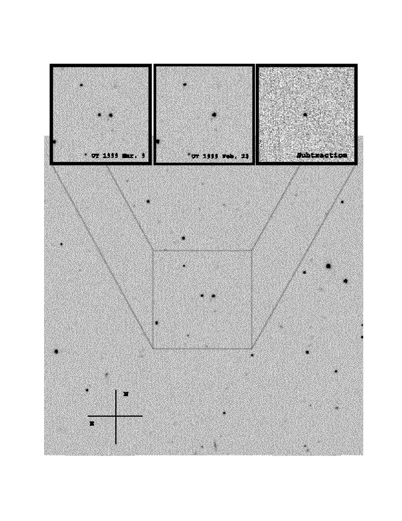
Figure 1: Discovery image of SN 1999aw taken on UT 1999 Mar. 9 on the KPNO 0.9-meter telescope. Image is $\sim 6\arcmin$ across ($0.423\arcsec$/pixel). Superimposed at the top are the discovery image, the template image (taken UT 1999 Feb. 23), and the subtraction. Algorithms used to produce the residual image are outlined briefly in Section 2.

The candidate supernova was photometrically confirmed on UT 1999 Mar. 10 in direct images obtained by R. Covarrubias at the Cerro Tololo Inter-American Observatory (CTIO) 0.9-meter telescope. The direct images showed that the object had not moved, within the limits of the seeing, in the time since its discovery. Figure 2 shows SN 1999aw 11 days after discovery, and 3 days after maximum light.

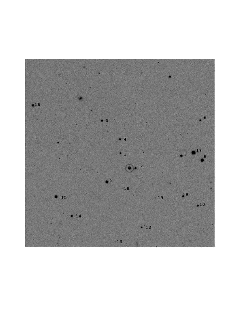
Figure 2: 240 sec exposure of SN 1999aw (and local photometric sequence) in B from CTIO 0.9-meter on UT 1999 Mar. 20.3. Circle indicates SN. Image is $\sim 7\arcmin$ across ($0.396\arcsec$/pixel). North is up, East is to the left.

The candidate was identified as a Type Ia supernova near maximum light from spectra obtained by A. Goobar, T. Dahlen, and I. Hook on UT 1999 Mar. 16.1 at the 2.6-meter Nordic Optical Telescope (NOT) using the Andalucia Faint Object Spectrograph and Camera (ALFOSC). Wavelength coverage was $\sim 4000-8000$Å with a resolution of 700 (or 430 km/s). A day later, L.-G. Strolger and R. C. Smith also obtained spectra at the CTIO 4.0-meter Blanco telescope (UT Mar. 17.3) using the R-C Spectrograph. The effective wavelength coverage was 3400 - 7500 Å, with an approximate resolution of 1000 (or 300 km/s). From these spectra (presented in Figure 3), M. M. Phillips confirmed the initial identification by Goobar et al., and based on the very small ratio of Si II$\lambda$5978 absorption relative to the Si II$\lambda$6355 line (see Nugent et al. 1995a), suggested that SN 1999aw was likely to be a luminous, slow-declining SN Ia.

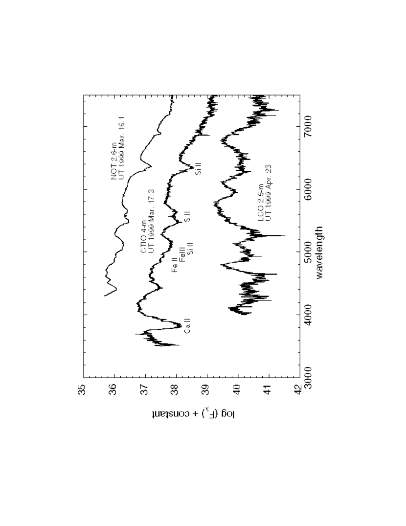
Figure 3: Spectral sequence of SN 1999aw. Confirmation spectra from NOT (upper spectrum) and CTIO (middle spectrum) were obtained near maximum light. Lower spectrum (From LCO) shows SN near initialization of the nebular phase. This was used to determine the redshift to SN 1999aw of $z=0.038\pm 0.001$.

3 Optical Spectroscopy

Although SNe Ia generally show similar spectral evolution (e.g., Branch et al. 1993), Nugent et al. (1995a) showed that a spectral sequence exists for SNe Ia which is analogous to the luminosity-decline rate relations. Specifically, certain spectral features show a systematic variation as a function of $\Delta$$m_{15}(B)$. Nugent et al. argued that this spectral sequence is due primarily to the differences in effective temperature which are presumably correlated with the amount of ⁵⁶Ni produced in the explosion.

At maximum light, spectroscopically normal SNe Ia exhibit strong Ca II H and K features near 3750 Å, and strong Si II$\lambda$6355 absorption which is blue-shifted by the high velocity of the expansion to appear near 6150Å in the rest frame of the event (Minkowski 1940, Pskovskii 1969, Branch & Patchett 1973). Excellent examples of normal SNe Ia are SNe 1981B, 1989B, 1992A, and 1994D. In general, there are two groups of the spectroscopically “peculiar” Type Ia SNe, also characterized near maximum light: SN 1991T-like events, and SN 1991bg-like events. 1991bg-like supernovae show wide absorption from 4150 - 4400 Å due to Ti II, and an enhanced 5800 Å feature (commonly attributed to Si II) in relation to Si II$\lambda$6355 (Filippenko et al. 1992, Leibundgut et al. 1993). The 5800 Å feature has been recently shown to be dominated by Ti II absorption (rather than Si II) in SN 1991bg-like SNe, and may even be considerably significant in spectroscopically normal SNe (Garnavich et al. 2001). Alternatively, 1991T-like SNe have prominent Fe II and Fe III features at maximum light, but little or no Si II, S II, or Ca II (Phillips et al. 1992). A week after maximum light, however, the Si II, S II and Ca II features develop, and the spectra become virtually indistinguishable from normal Type Ia.

Nugent et al. (1995a) showed that 1991bg-like events correspond to the low-temperature end of the SNe Ia spectroscopic sequence (a fact supported by Garnavich et al. 2001), while 1991T-like events are associated with the highest effective temperatures. Normal SNe Ia inhabit the middle range of the sequence, where Ti II absorption is weak, the ratio of Si II$\lambda$6355 to Si II$\lambda$5800 is relatively high, and the Ca II H and K trough is strong. Hence it may be more precise to refer to 1991bg-like and 1991T-like events as the extremes in a spectroscopic sequence rather than as “peculiar” events.

Li et al. (2001) also document a variation of SN 1991T-like events for supernova spectra that resemble SNe 1999aa, 1998es, and 1999ac. These SN 1999aa-like supernovae are similar to 1991T-like SNe supernovae, but show some Si II$\lambda$6355 prior to maximum light (stronger than in 1991T-like SNe, but weaker than in normal Type Ia SNe), and clearly present Fe II and Fe III lines near maximum light. They also exhibit strong Ca II H and K lines.

The spectra of SN 1999aw obtained by Goobar et al. (Mar. 16.1) and Strolger and Smith (Mar. 17.3) are displayed in Figure 3, and clearly show a SN Ia at or near maximum light. In Figure 4, the Mar. 17.3 spectrum is compared with maximum-light spectra of four other SNe Ia with similarly-slow decline rates. SN 1990O was observed by Hamuy et al. (1996c), and in spectra as early as 8 days before maximum clearly showed strong Si II$\lambda$6355 absorption (Phillips et al., in preparation). SN 1992P was also observed by Hamuy et al. (1996c). Although nothing is known about its spectrum a week or more before maximum, the spectrum plotted in Figure 4 also shows strong Si II$\lambda$6355 absorption at maximum. SN 1999aa is the prototype of the 1999aa-like events described in the previous paragraph. Overall, the spectrum of this supernova (reproduced from Fig. 5 of Li et al. 2001) is very similar to those of SNe 1990O and 1992P, except that the Si II$\lambda$6355 absorption is noticeably weaker. At the bottom of Figure 4 we plot the spectrum of SN 1999aw obtained on Mar. 17.3. The similarity to the spectrum of SN 1999aa is striking, with the only significant differences being the somewhat broader lines and stronger Ca II absorption of SN 1999aw. In section 4 we shall give further evidence for such a link based on the optical and IR light curves.

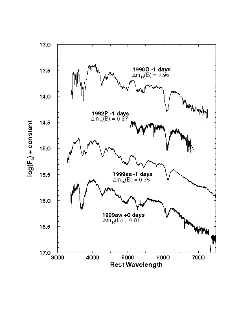
Figure 4: Comparison of SN 1999aw spectrum to other supernovae near maximum light. SN 1999aw is more similar to SN 1999aa, than to SNe 1990O or 1992P.

On UT 1999 Apr. 23, M. M. Phillips obtained a spectrum of SN 1999aw using the duPont 2.5-m telescope at Las Campanas Observatory (see Figure 3). The WFCCD was used in spectroscopic mode at a resolution of 630 (or 480 km/s) and the data covered the approximate wavelength range of 3750$-$9250Å. The date of observation corresponds to an epoch of 37 days after maximum light. By this late epoch, SNe Ia have begun their nebular phase, where their photospheres have essentially disappeared and their spectra become montages of blended emission features (Wells et al. 1994). The peaks of these features, fortunately, do not change substantially with time, hence they can be used to determine the redshift of SN 1999aw relative to SNe Ia with well-determined host galaxy redshifts and late epoch spectra.

We compared the UT 1999 Apr. 23 spectrum to spectra of SNe 1992bc, 1989B, and 1992A taken at epochs of +37 days, +36 days, and +36 days past maximum light respectively, and determined the relative shift between them. Using the host galaxy redshifts given in NED, we calculated the redshift for SN 1999aw of 0.0392, 0.0372, and 0.0380, respectively. The mean result is $z=0.038\pm 0.001$ which we will use throughout this paper.

An additional late-time spectrum of SN 1999aw was obtained by M. Hamuy on UT 1999 May 19 using the NTT 3.6-m telescope at European Southern Observatory (see Figure 5). The EMMI was used in spectroscopic mode at a resolution of 600 (or 500 km/s) and an approximate wavelength range of 4600$-$8600Å. The date of this observation corresponds to an epoch of 64 days after maximum light, at which time the supernova was more “nebular” than in previous epochs, with more pronounced emission features. Recalculating the redshift to SN 1999aw based on the centers of Fe III$\lambda$4658 and Co III$\lambda$5890 results in $z=0.037\pm 0.002$, which is consistent with the redshift determined from the UT 1999 Apr. 23 spectrum.

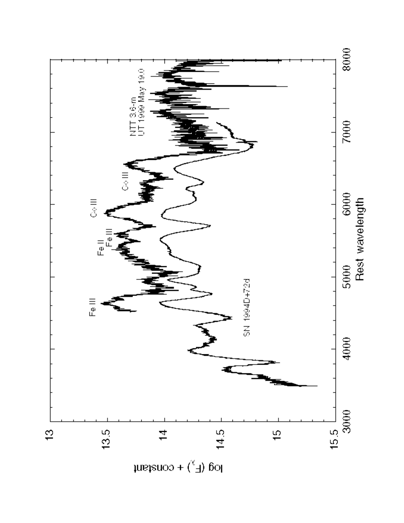
Figure 5: Additional late-time spectrum of SN 1999aw from NTT 3.6-m taken UT 1999 May 19.0. Spectrum is shown at rest wavelength. Nebular emission lines such as Fe III$\lambda$4658 and Co III$\lambda$5890 were used to calculate $z=0.037\pm 0.002$, which is consistent with $z=0.038\pm 0.001$ as derived from LCO 2.5-m spectrum (see Figure 3). A spectrum of SN 1994D at $+$72 days from maximum is also shown for comparison.

4 Photometry and lightcurves

4.1 Optical Photometry

Our search techniques provided bulk SNe detections, and therefore we could schedule sufficient follow-up observations to produce well-sampled light curves. Following the search campaign, we obtained several optical images using scheduled time on the CTIO 0.9-meter, 1.5-meter, and 1.0-meter (YALO) telescopes. The scheduling was planned such that the sampling would produce at least one data point every three nights, in each of the BVRI filters, for at least 30 days after the discovery. We also obtained scheduled observations from various other telescopes. Data were reduced (bias subtracted and flat-field corrected) using standard IRAF packages for reducing multiple and single amplifier data. A shutter correction was measured for CTIO 0.9-meter, and 1.5-meter data, and applied to short exposures ($<20$ seconds).

The brightness of SN 1999aw, and its lack of host galaxy-light contamination, allowed accurate aperture photometry to be performed, without the need for late-time galaxy-light subtraction. Using the DAOPHOT II package (Stetson 1992), data from photometric nights were compared with stars from tabulated standard fields (Landolt 1992). Interactive iterative solutions were made to construct a growth curve and mean aperture correction for stars on each frame. Solutions were then calculated for the coefficients of the linear color and airmass terms to convert from natural to standard apparent magnitudes (see Appendix, Tables A7 and A8). A set of local field standards stars was then produced around SN 1999aw (see Figure 2), tied to the Landolt (1992) standard stars observed. Table 1 contains the sequence of local photometric standards, coordinate offsets in arcseconds from SN 1999aw (based on the WCS), and the photometric indices of these standards along with the mean errors. Data of the SN from all other nights were compared to the data from the photometric nights using these standardized local field stars. Table 2 contains the epochs of observation of SN 1999aw, and the BVRI photometry along with the photometric errors. These optical lightcurves are plotted in Figure 6.

As expected from the identifying spectra, SN 1999aw did indeed dim after peak at a slower-than-average rate. We performed a Monte Carlo simulation to randomly vary each data point within the photometric error 300 times, each time least-squares fitting a 3rd order polynomial to the peak of the B band lightcurve. Averaging the solutions to the simulations led to the B-band peak of $B_{max}=16.88\pm 0.01$ on JD 2451254.7$\pm 0.3$ (UT Mar. 17.2), and a decline rate within the first 15 days after maximum light of $\Delta$$m_{15}(B)=0.80\pm 0.03$. Similar Monte Carlo simulations were performed on the V, R and I lightcurves, the results of which are summarized in Table 3. Using $z=0.038$ and assuming $H_{o}=65$ km/s/Mpc, we derive the absolute magnitudes of $M_{B}=-19.48\pm 0.11$, $M_{V}=-19.52\pm 0.11$, $M_{R}=-19.52\pm 0.11$, and $M_{I}=-19.04\pm 0.12$, correcting only for Galactic extinction in the direction of SN 1999aw using values of $A_{B}=0.14$, $A_{V}=0.11$, $A_{R}=0.09$, and $A_{I}=0.06$ (Schlegel, Finkbeiner, & Davis 1998).

4.2 Infrared Photometry

Infrared imaging of SN 1999aw was obtained over a 50-day period, beginning at the epoch of B maximum, using the Swope 1-meter and duPont 2.5-meter telescopes at Las Campanas Observatory (LCO), and using the VLT at European Southern Observatory. These data were taken in the J_s, H, and K_s bandpasses.

The LCO infrared images were reduced with IRAF using standard techniques. Briefly, the steps consisted of 1) application of a correction for the slightly non-linear response of the NICMOS detector, 2) subtraction of dark images of the same exposure time as the supernova images, 3) division by a twilight flat field, 4) subtraction from each individual exposure of a sky image created from the dithered images of the supernova, and 5) shifting and summing the individual images to create a final “mosaic” image of the supernova field. DAOPHOT II was used to obtain PSF photometry, construct growth curves, and to set up local standards using observations on photometric nights of the Persson et al. (1998) standard stars. As the Persson et al. standards were established using the same instrument/detector/filters employed for the Swope telescope observations of SN 1999aw, no color corrections were applied to the supernova magnitudes. The duPont IRC observations are probably also very nearly on the same system, but this may not be the case for the duPont CIRSI and VLT data. It has been noticed that although the VLT/ISAAC transmission curves are fairly similar to the LCO filters in H and K_s, the J_s filter is significantly narrower and therefore the J_s-band observations can be quite different from the LCO system. We hope to eventually derive appropriate transformations for the latter data to the Persson et al. photometric system; in the absence of such information, no color corrections for these data are made in the present paper.

Table 4 lists the local standard star photometry (using the same numbering system as in the optical), Table 5 contains the epochs of observation of SN 1999aw with photometric errors, and Figure 6 shows the resulting infrared light curves.

Figure 6: Optical and IR lightcurves of SN 1999aw with photometric errors. Template curves for B,V, and I are from the spectroscopically normal SN 1992al, which had a mid-range decline rate of $\Delta$$m_{15}(B)=1.11$ (Hamuy et al. 1996d). Templates for J_s, H, and K_s from fiducial curves of Elias et al. (1985b). Both the optical and IR templates have been adjusted for a redshift of $z=0.038$.

4.3 K-Corrections and Time Dilation

At $z=0.038$, the redshift of SN 1999aw is large enough that it is important to correct the flux received in a given filter to that which would have been received if the event occurred at nearly zero redshift. If spectroscopic data were available for each epoch a direct image was obtained, corrections could be made to the flux received in each passband, or K-corrections, by determining the change in brightness in the transmission curves of those passbands as the spectra are shifted from the observed reference frame to the rest frame. Corrections would be applied as $m(z=0,\tau)=m(z,\tau)-K(z,\tau)$, where $\tau$ is the epoch from maximum light. As this extensive spectral data is unavailable, we employ a method similar to that of Nugent et al. (2002, in prep). Here several epochs of spectra for SN 1999aw spanning the optical regime were used to produce the K-correction by manipulating the spectral energy distribution, producing synthetic photometry on a particular date to match the corresponding observed colors of SN 1999aw. We interpolate and extrapolate these few K-terms to derive K-terms for all epochs of photometric observation. The uncertainties from this method, based on the photometric data and the associated uncertainties for SN 1999aw, are less than 0.02 magnitudes for a given epoch.

In at least B and V, the K-terms are in good agreement with the values produced in a pure application of the method of Nugent et al. (2002), and with the values tabulated in Hamuy et al. (1993) for a SN Ia at $z=0.04$. However, in I there is a significant difference from yet unpublished K-terms determined from other nearby SNe Ia. This difference is caused by the delay (or “stretch”) in the I-band lightcurve of SN 1999aw, which is consistent with a possible trend among bright slow-declining 1991T/1999aa-like SNe Ia in which the IJHK lightcurves evolve at a slower rate than other SNe Ia (see Section 5.2). This difference in photometric (and plausibly spectroscopic) evolution exemplifies the danger in applying K-corrections calculated from SNe Ia with radically different decline rates.

Applying the derived K-corrections to the photometric data for SN 1999aw, and correcting the observed passage of time by a factor of $(1+z)^{-1}$ for time dilation, produced a rest frame apparent magnitude lightcurve that was not that different from the observed lightcurve, with $\Delta$$m_{15}(B)=0.81\pm 0.03$. We have not attempted to make K-corrections for the near-IR data because we do not have IR spectra for SN 1999aw, nor are there yet sufficient libraries of IR spectra for other SNe Ia.

5 Analysis and Discussion

5.1 B-band Template Fits

The lightcurves of SN 1999aw are remarkable for how much slower they evolve compared to the template curves of a typical decline-rate SNe Ia (see Figure 6). This is evident not only in the slow initial decline rate of $\Delta$$m_{15}(B)=0.81$ (the mean decline rate of SNe Ia is $\Delta$$m_{15}(B)\sim 1.1$), but in the delay of the second maximum in I, J_s, H, and K_s.

The B-band lightcurve is particularly interesting in that its “shape” is subtly different than that for typical SNe Ia. One parameter LWR relations such as the $\Delta$$m_{15}(B)$ suggest that a B-band lightcurve template can be made to fit the B-band lightcurve of a SN by applying a time delaying “stretch” factor to the epochs of observation, and the related magnitude offset (Perlmutter et al. 1997). However, Strolger et al. (2000 & 2003a) show that B-band template lightcurves built from well-sampled spectroscopically normal SNe Ia fit poorly to the B-band lightcurves of 1991T/1999aa-like supernovae, even when stretched to fit the observed lightcurve in early epochs (By “normal”, we mean those those SNe Ia which displayed strong Si II$\lambda 6355$ absorption at least 5 days before B-band maximum).

The Strolger et al. (2000 & 2003a) analysis was conducted on a few SNe that were 1) spectroscopically identified at least 5 days before maximum light, and 2) frequently observed with well sampled B-band lightcurves from just prior to maximum light to around the $+$80 day epoch. The low-order mean difference between the template curve and the supernovae lightcurves from the beginning of the exponential phase (after the $+$25 day epoch) was determined for each supernova in the sample:

$$\delta_{ave}=\sum_{+25}^{+80}\frac{m(t)-m_{T}(t^{\prime})}{N}$$ (1)

Observations made at some epoch, $m(t)$, were compared to the time stretched template curve, $m_{T}(t^{\prime})$, and then averaged over the number of observations ($N$) from the $+$25 day to $+$80 day epochs.

Results of the analysis show that spectroscopically normal SNe Ia exhibit little to no difference from the template curve during the exponential phase, whereas 1991T/1999aa-like SNe Ia show a substantial overbrightness during this phase. The analysis, when performed on SN 1999aw, produced a result consistent with that of the 1991T/1999aa-like SNe.

Figure 7 shows four SNe spectroscopically similar to SNe 1991T and/or 1999aa (including SN 1999aw), along with the normal SNe Ia template, stretched in time to fit the lightcurves within the first 15 days past maximum light. The template does not fit well to the data past around the $+25$ day epoch, and the data are systematically brighter than the template from that epoch.

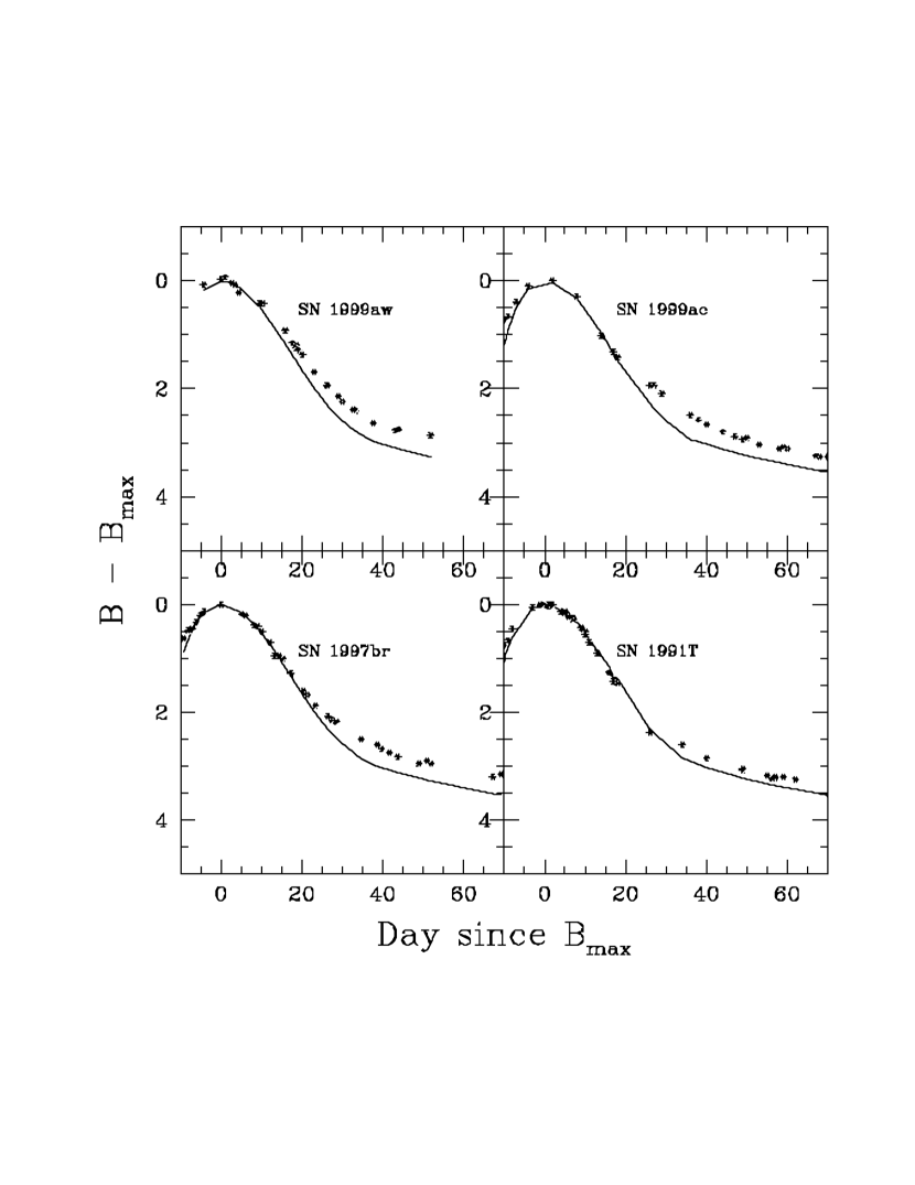
Figure 7: B-band lightcurves of four 1991T/1999aa-like supernovae, scaled to B_max. Solid line is a Template for spectroscopically normal Type Ia SNe, stretched along time axis to fit observations between peak and $+$15 days past maximum light.

In the future, with more examples of 1991T/1999aa-like SNe, this analysis may lead to photometric method that, in addition to spectroscopy, indicate the possible 1991T/1999aa-like peculiarity of supernovae.

5.2 Color Curves

SNe Ia show a impressive uniformity in their intrinsic colors in late epochs after maximum light. As Lira (1995) and Riess et al. (1996) independently showed, SNe Ia with $0.85\lesssim$$\Delta$$m_{15}(B)$$\lesssim 1.90$ and little or no reddening from their host galaxies have very uniform $B-V$ color evolution from $+$30 to $+$90 days after maximum light. Krisciunas et al. (2000) also observe uniformity in the V$-$Near IR color evolution of spectroscopically normal SNe Ia with mid-range decline rates from $-$9 days to $+$27 days past maximum light.

Figure 8 shows the evolution in multiple colors of SN 1999aw, corrected for Galactic reddening assuming an excess of $E(B-V)=0.032$ (Schlegel, Finkerbeiner, & Davis 1998). The left-hand side panels of Figure 8 show the optical color evolution, along with some example SNe (zero-reddening corrected) for comparison. The solid line in the plot of the evolution of $B-V$ in this figure represents the zero-reddening least-squares fit derived by Lira (1995). SN 1992al is included to show the evolution of a typical SNe Ia, while SN 1992bc is a slow-declining SNe Ia ($\Delta$$m_{15}(B)=0.87$) but with normal pre-maximum light spectra. SNe 1991T and 1999aa, the prototypical 1991T/1999aa-like SNe, have color evolutions nearly parallel to the Lira (1995) line, thus showing that the uniformity holds for some spectroscopically extreme SNe Ia.

Figure 8: Color curves of SN 1999aw with photometric errors. B$-$V curve includes Lira zero-reddening relation (Phillips et al. 1999). V$-$Near IR curves include zero-reddening relations from Krisciunas et al. (2000) for Type ia SNe with mid-range decline rates.

This color uniformity has proven useful as an indicator of host galaxy reddening, which has been important to revising the LWR relations (Phillips et al. 1999). We have used the recipes in Phillips et al. (1999) to determine the host galaxy reddening for SN 1999aw. The analysis gave $E(B-V)_{tail}=-0.20\pm 0.05$, $E(B-V)_{max}=0.12\pm 0.10$, and $E(V-I)_{max}=-0.11\pm 0.09$, which when averaged, resulted in a negative color excess, implying zero host galaxy reddening. Clearly the negative value of $E(B-V)_{tail}$ is heavily influenced by the anomalous $B-V$ color evolution of SN 1999aw; specifically, for most of the period from $+$40 days to $+$60 days SN 1999aw was considerably bluer than the Lira (1995) zero-reddening fit, and perhaps evolving with a steeper slope.

As SN 1999aw was spectroscopically similar to SN 1999aa, we might have expected that its color evolution would be similar to SN 1999aa and/or SN 1991T, both of which appeared generally bluer than SN 1992bc in $V-R$ and $V-I$. In SN 1999aw, the bluer $V-R$ and $V-I$ evolution were caused by the delay in the appearance of the second lightcurve maximum, which was more clearly seen in redder passbands (see Figure 6), and therefore is accentuated in the $V-R$ and $V-I$ curves. SN 1999aw also appeared bluer than SN 1999aa and SN 1991T in $V-R$ and $V-I$, which perhaps was an effect of SN 1999aw having a much slower decline rate than both SN 1999aa and SN 1991T.

The $V-J_{s}$ and $V-H$ curves for SN 1999aw are also considerably bluer than the zero-reddening fits from Krisciunas et al. (2000) in the period after $+$10 days (right-hand side panels of Figure 8). The trend in the period prior to $+$10 days in the $V-J_{s}$ curve also seems to be different than the fit from Krisciunas et al. It appears that one could apply a “stretch” to the Krisciunas lines to force them to fit the SN 1999aw data, that is to say there is an apparent delay in the $V-J_{s}$ evolution. This again is due to the apparent delay of the second maximum in the I, J_s, H, and K_s lightcurves. Note, however, that the $V-J_{s}$, $V-H$, and $V-K_{s}$ colors in this figure may change somewhat once K-corrections for the IR bandpasses become available.

5.3 Bolometric lightcurve, Maximum Luminosity, and ⁵⁶Ni Mass Estimate.

As nearly all of the bolometric luminosity of a typical Type Ia supernova is emitted in the range of 3000 to 10000Å (Suntzeff 1996), the integrated flux in the UBVRIJ_sHK_s bandpasses provides a reliable and meaningful estimate of the bolometric luminosity, which is directly dependent on the amount of nickel produced in the explosion.

The BVRIJ_sHK_s data were used to calculate “uvoir” bolometric fluxes using the techniques described in Suntzeff (1996) and Suntzeff and Bouchet (1990). A table of UBVRIJ_sHK_s data was made by linearly interpolating the J_sHK_s data to the optical dates. For some of the missing optical and J_s and H data, we added photometry based on spline fitting of the data to the date of the missing data. We have added on U data because the optical ultraviolet adds significant flux to the early time bolometric light curve. There is little high-quality U data for Type Ia supernovae due to the generally poor ultraviolet sensitivity of the present generation of CCDs. We have instead relied on $U-B$ photometry from photoelectric measurements. For dates past $+$9 days from B maximum, we have used the $U-B$ data of SN 1972E from Lee et al. (1972) and Ardeberg & de Groot (1973). For dates before $+$9 days from B maximum we have used the $U-B$ data for SN 1980N from Hamuy et al. (1991), and for SN 1981B compiled by Cadonau & Leibundgut (1990). The $U-B$ for these supernovae were corrected to the reddening of SN 1999aw using the reddening values in Phillips et al. (1999) and a value of $E(U-B)/E(B-V)=0.72$ from Cardelli et al. (1989). The U photometry of SN 1999aw was then estimated from spline fits to the $U-B$ data of these supernovae combined with our B data of SN 1999aw.

We then converted the broadband magnitudes to equivalent monochromatic fluxes at the effective wavelengths of Vega (Bessell 1979, 1990; Bessell & Brett 1988). A magnitude scale of $(U,B,V,R,I)=0.03$ and $(J,H,K)=0.0$ was used for Vega. The monochromatic fluxes were then scaled to the magnitude of the supernova, dereddened by $E(B-V)=0.032$ using the reddening law of Cohen et al. (1981), and corrected to intrinsic fluxes using a distance modulus of 36.28 based on a Hubble flow with a Hubble constant of 63.3 km/s/Mpc (Phillips et al. 1999). These fluxes were then integrated using a simple trapezoidal integration. We added on a Rayleigh-Jeans extrapolation to zero frequency to the reddest flux point. We extrapolated to the ultraviolet by adding a flux point at 3000Å with zero flux.

We correct the derived bolometric lightcurves for time dilation effects, and plot them in Figure 9. The UBVRI and the UBVRIJ_sHK_s integrations track each other well, except that the inflection points around days 20-45 are more pronounced in the UBVRIJ_sHK_s integrations. Similar inflection points were noted by Suntzeff (1996) and are indicative of significant flux redistributions which may be related to rapid changes in the wavelength dependence of the opacities (Pinto & Eastman 2000 a & b). The peak bolometric luminosity is about $L_{bol}=1.51\times 10^{43}$ erg s^-1.

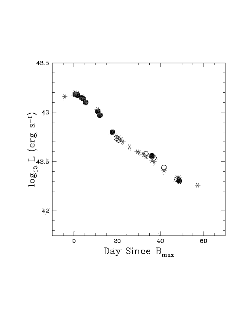
Figure 9: The bolometric lightcurve of SN 1999aw, constructed from the integrated flux in the B, V, R, I, J_s, H, and K_s passbands, and corrected for time dilation. Stars show the bolometric curve in UBVRI, while open circles are in UBVRIJ_sH, and filled circles are in UBVRIJ_sHK_s.

It is fairly straightforward to derive the nickel mass produced in the explosion from the bolometric luminosity at peak. At maximum light, photons escape the surface at a rate which is equal to the radioactive energy input produced primarily by the ⁵⁶Ni decay, and thus it is also related to the ⁵⁶Ni synthesized in the explosion (Arnett 1982, Nugent et al. 1995b, Pinto & Eastman 2000a).

Contardo et al. (2000) calculate the luminosity and nickel mass for several SNe Ia from UBVRI bolometric peak fluxes. Using the same method, and assuming a rise time of 17 days to bolometric peak for consistency with Contardo, et al., we derive an initial nickel mass of $M_{Ni}=0.76M_{\odot}$ for SN 1999aw. This is brighter and more nickel massive than many of the normal Type Ia SNe discussed in Contardo, et al., and it is comparable in brightness and nickel mass to SN 1991T (see Table 6). However as they note, a number of the SNe Ia in their study do not have U-band data available at peak, and therefore they have developed a correction curve based on data from the very well-sampled SN 1994D. Although this SN was spectroscopically normal, it did have some rather unusual features, including an unusually blue $U-B$ color at maximum light. Additionally, Riess et al. (1999) have shown that the characteristic rise time of SNe Ia is $19.5\pm 0.2$ days, and that brighter and slower declining SNe Ia have longer rise times. For the peak magnitude and decline rate observed in SN 1999aw, we expected a rise time of $\sim 20$ days. Using this value, we derive an alternative initial nickel mass of $M_{Ni}=1.07M_{\odot}$.

There are a number of additional uncertainties in both the calculated luminosity, and the derived nickel mass. The first is the assumption that more than 80% of the true bolometric light is emitted in the optical regime, that less than 10% can be expected in the UV below 3200Å, and that no more than 10% (in early epochs) from JHK (Suntzeff 1996, Elias et al. 1985, Contardo et al. 2000). In comparing our derived UBVRIJ_sHK_s and UBVRI bolometric fluxes, we find the IR contribution to be only a few percent ($\sim 1\%$ at early epochs, $\sim 5\%$ after 35 days past $B_{max}$). We have not accounted for the space ultraviolet flux.

Also, as we will discuss further in Section 6, we do not have much information about the host galaxy of SN 1999aw. Although we have compensated for extinction and reddening due to our own galaxy, it difficult to do the same for the host galaxy. However, as the $B-V$ color of SN 1999aw is nearly zero at maximum light, as it would be for an unreddened Type Ia SN (Phillips et al. 1999; Garnavich et al. 2001, in Figure 15), we have assumed that the extinction due to the host must be negligibly small.

6 The Host Galaxy of SN 1999aw

Another approach to understanding SN 1999aw can be to investigate its host galaxy. The metallicity of the progenitor may be related to the environment of the event (Hamuy et al. 1995). However, the apparent low luminosity of the galaxy has made it very difficult to study. As earlier stated, there was no obvious host galaxy in the template images nor in subsequent photometry. On UT 2000 Feb. 12, L. Strolger, P. Candia, J. Seguel, and A. Bonacic obtained deep images of the SN 1999aw field using the CTIO 1.5-meter telescope. Pairs of long exposures were taken in the same standard BVRI filters as were used in the photometry of SN 1999aw (The combined exposure times were 1200 seconds for B, V, and I, and 1440 for R). Zero points in each filter were found by comparison of standards fields taken on the same evening, with tabulated standard magnitudes. No clear detection (to a 3-$\sigma$ level) was made of a galaxy at or near the position of SN 1999aw in these deep images (see Figure 10).

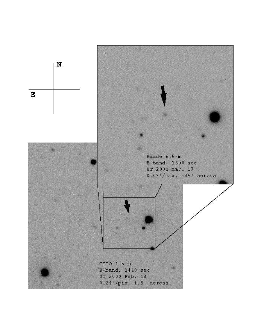
Figure 10: Deep imaging of the SN 1999aw field. Host is visible in the Magellan 6.5-meter data.

A second attempt to detect the host was made on UT 2001 Mar. 17 by A. Szentgyorgyi, and on UT 2001 Mar. 18 by M. Mateo, A. Athey, and K. von Braun, both using the Baade 6.5-meter telescope at Las Campanas Observatory and the Magellan Imaging camera (MagIC). They obtained deep exposures for a combined 1600 sec in B, 1400 sec in V, and 900 sec in I of the SN 1999aw field. These deep images did reveal a resolved galaxy, with FWHM of 0.6″, only slightly broader than the seeing (0.42″). The central brightness (within 1.5″ radii) were $B=24.2\pm 0.2$, $V=23.8\pm 0.2$, and $I=24.1\pm 0.9$ magnitudes. The radial growth curve for the galaxy was very steep in all passbands, and heavily contaminated by background noise in the image. Therefore, we assume the 1.5″ magnitudes are the best estimates of the total light in the galaxy. Absolute values of $M(B)_{T}=-12.2\pm 0.2$, $M(V)_{T}=-12.5\pm 0.2$, and $M(I)_{T}=-12.2\pm 0.9$ were calculated assuming $H_{o}=65$ km/s/Mpc and correcting only for Galactic extinction.

Coincidentally, the low luminosity dwarf galaxy IC 4182 hosted type Ia supernova SN 1937C, also with slow decline rate ($\Delta$$m_{15}(B)=0.87$). Although Branch et al. (1993) indicate that spectra from Minkowski (1939 & 1940) of SN 1937C seem to show a normal Type Ia SN, there may be some question as to whether or not the Si II$\lambda$6355 feature was relatively weak at early epochs, possibly indicating a similarity to SN 1999aa. Using the measured CCD photometry of IC 4182 from Makarova (1999), and the Cepheid distance modulus for the galaxy calculated by Saha, et al. (1994) and correcting for Galactic extinction, we determined its absolute magnitude to be $M(B)_{T}=-16.4\pm 0.02$, $M(V)_{T}=-16.8\pm 0.2$, and $M(I)_{T}=-17.6\pm 0.2$. The SN 1999aw host galaxy is significantly fainter (by 4.2, 4.3, and 5.5 magnitudes in B, V, and I, respectively).

The error in these observations, especially in I, make it difficult to estimate color differences for the host galaxy, however, using the magnitudes above yields $(B-V)_{o}=0.31\pm 0.28$ and $(V-I)_{o}=-0.35\pm 0.92$. Assuming $(B-V)_{o}$ better exemplifies the color trend, the galaxy would appear to be fairly blue in comparison to dwarf galaxies in the local group (see Table 4 and Fig. 3 of Makarova 1999).

Initial studies of SNe Ia characteristics and their relation to their host galaxies have been conducted by Ivanov, Hamuy, & Pinto (2000) and Hamuy et al. (2000). Their studies show:

• The distribution of SNe Ia decline rates (and therefore brightness) changes considerably with host galaxy morphological type. Earlier Hubble type galaxies (such as ellipticals and S0 spirals) produce faint fast-declining SNe Ia, and late type galaxies (Sa$-$Irr) tend to produce bright slow-declining SNe Ia.

• SNe Ia decline rates also change with $B-V$ color of the host galaxy. Bright SNe Ia occur more frequently in bluer environments.

• Bright SNe Ia occur more frequently in less luminous galaxies.

It is difficult, however, to determine how these color$-$luminosity correlations relate to age and metallicity effects. Integrated galaxy luminosities seem to correlate with metallicity (Henry & Worthy 1999), and both the sample of galaxies from Hamuy et al. (2000) and the sample of dwarf galaxies from Makarova (1999) seem to indicate that the least luminous galaxies are also the bluest. As bluer galaxies are also younger, perhaps the brightness distribution of SNe Ia with $B-V$ color is an age effect, suggesting that younger environments produce bright slow-declining SNe Ia. Alternatively, it is plausible that the SNe Ia brightness$-$color correlation is just a reflection of the SNe Ia brightness$-$host galaxy luminosity trend, which may be a metallicity effect indicating that metal-poorer environments produce the brightest SNe Ia.

Nonetheless, observations of SN 1999aw and its host galaxy are consistent with these trends in that the host was faint and blue [among the faintest 10% in $M(B)$, and the bluest 15% in $(B-V)$ of the Makarova (1999) sample], and that it produced a bright slow-declining SN Ia.

7 Summary

Our photometric and spectroscopic study of SN 1999aw indicate that SN 1999aw was probably a 1999aa-like event. The light curve decline rate is among the slowest observed at $\Delta$$m(B)_{15}=0.81\pm 0.03$. At the redshift of $z=0.038$, it is also among the brightest Type Ia, with $M_{B}=-19.45\pm 0.11$, $M_{V}=-19.50\pm 0.11$, $M_{R}=-19.38\pm 0.11$, and $M_{I}=-18.97\pm 0.12$. Although luminous, these magnitudes are slightly less (by a few tenths of a magnitude) than one might expect from the trends of absolute magnitude versus decline rate or $\Delta$$m_{15}$ (See Figure 11 of Krisciunas et al. 2001). Perhaps this suggests that there is some host galaxy extinction that needs to be accounted for. Or it is possible that SN 1999aw is simply slightly less luminous than expected, and therefore may be indicating a possible downward curve to the relations in Fig. 11 for the slowest-declining SNe Ia (similar to the downward curve recently determined by Garnavich et al. (2001) for fast-declining SN 1991bg-like SNe Ia).

It is thought that the brightness and decline rate of Type Ia are dependent on the metallicity of the progenitor, and additionally on the opacity in the atmosphere of the event (Hoflich et al. 1998, Pinto and Eastman 2000a & b, Mazzali et al. 2001). The derived luminosity of $1.51\times 10^{43}$ erg s^-1, and ⁵⁶Ni mass of $0.76M_{\odot}$ for SN 1999aw are both relatively high, but are consistent with what can be expected for a SN Ia with the observed decline rate, as inferred from the trend between $\Delta$$m_{15}(B)$ and ⁵⁶Ni mass evident in Table 6.

The observations made at the Baade 6.5-meter have provided some very interesting information on the host galaxy of SN 1999aw. The derived absolute magnitudes seem to indicate that it is among the intrinsically faintest and bluest dwarf galaxies observed. This may indicate that the galaxy consists of either a young population of stars, or is a fairly metal-poor environment. It will be necessary to eventually obtain deeper images with large telescopes such as the Magellan 6.5-meter or the VLT to obtain sufficient signal-to-noise to put more accurate constraints on not only the colors of this galaxy, but its structure as well. The discovery of SN 1999aw exemplifies an advantage of magnitude limited field searches over galaxy-targeted searches. It is presently unclear how many supernova similar to SN 1999aw occur at low redshift, and with the biases associated with current targeted surveys we are less likely to detect them. As more magnitude limited field searches commence, relations between low luminosity (and probably low metallicity) galaxies and the supernova types that occur in them can be accurately determined. This will not only place constraints on Type Ia supernova progenitor models, but help to clarify the possibility of supernova “evolution” which may explain the difference in SN 1991T-like event rates between the low and high-$z$ surveys (Li et al. 2001).

Appendix A Photometric Transformation Equations

Optical aperture photometry was performed using the DAOPHOT II package (Stetson 1992). 14″ diameter apertures were used and were corrected by an iterative growth curve to a nearly infinite diameter. Standard fields were observed on 8 photometric nights on the CTIO 0.9-meter, and 7 photometric nights on the CTIO 1.5-meter. Caution was taken to observe fields at various airmasses in all filters. The data from 50 stars were compared to tabulated values (Landolt 1992) and solutions were found for the coefficients of the linear color and airmass terms in the photometric transformation equations (see Table A7 and A8). The equations were then used to transform the natural magnitudes of the local standard stars to standard magnitudes (see Table 1).

Table 1: Local Standard Indices

Star	E (″)	N (″)	V	B$-$V	V$-$R	R$-$I	V$-$I	NB	NV	NR	NI
1	$-$13.5	0.6	17.138 (0.015)	1.346 (0.033)	0.861 (0.022)	0.846 (0.022)	1.707 (0.020)	23	20	21	21
2	49.7	$-$30.0	16.67 (0.014)	1.95 (0.023)	0.373 (0.020)	0.339 (0.023)	0.712 (0.022)	23	20	19	21
3	19.7	33.1	18.477 (0.028)	0.7 (0.049)	0.406 (0.038)	0.39 (0.038)	0.795 (0.039)	17	16	15	17
4	20.4	63.4	17.587 (0.021)	0.856 (0.035)	0.486 (0.027)	0.433 (0.024)	0.919 (0.027)	23	22	19	21
5	58.9	104.2	17.83 (0.019)	0.728 (0.035)	0.428 (0.028)	0.4 (0.029)	0.828 (0.028)	22	19	18	20
6	$-$154.8	103.7	18.178 (0.028)	0.691 (0.045)	0.394 (0.041)	0.378 (0.038)	0.772 (0.037)	19	18	17	17
7	$-$112.5	26.6	17.38 (0.018)	0.555 (0.028)	0.372 (0.026)	0.378 (0.025)	0.75 (0.024)	21	20	19	19
8	$-$157.6	16.1	15.65 (0.010)	0.961 (0.018)	0.547 (0.014)	0.476 (0.012)	1.024 (0.012)	17	16	15	17
9	$-$116.0	$-$62.1	17.488 (0.018)	0.938 (0.033)	0.526 (0.026)	0.457 (0.024)	0.983 (0.025)	20	19	18	18
10	$-$147.8	$-$83.4	18.201 (0.027)	0.59 (0.043)	0.358 (0.039)	0.351 (0.039)	0.708 (0.037)	21	20	19	19
11	$-$122.9	$-$196.0	15.632 (0.017)	1.019 (0.027)	0.411 (0.025)	0.377 (0.024)	0.788 (0.023)	12	11	10	10
12	$-$25.6	$-$129.3	18.529 (0.028)	0.773 (0.048)	0.463 (0.040)	0.442 (0.041)	0.905 (0.041)	19	18	17	17
13	51.6	$-$190.1	16.958 (0.016)	0.648 (0.025)	0.393 (0.024)	0.384 (0.025)	0.777 (0.023)	17	16	15	15
14	126.2	$-$104.2	18.092 (0.026)	0.45 (0.038)	0.326 (0.040)	0.321 (0.043)	0.647 (0.040)	19	16	17	17
15	160.3	$-$61.6	16.279 (0.012)	2.387 (0.021)	0.515 (0.021)	0.452 (0.024)	0.967 (0.021)	17	14	15	15
16	208.7	138.7	17.369 (0.015)	0.576 (0.023)	0.356 (0.026)	0.346 (0.029)	0.702 (0.025)	9	9	8	7
17	$-$139.3	33	15.052 (0.009)	0.559 (0.016)	0.334 (0.013)	0.333 (0.013)	0.667 (0.013)	21	20	19	19
18	14.0	$-$43.7	20.951 (0.061)	0.672 (0.093)	2.037 (0.073)	0.579 (0.062)	2.616 (0.077)	4	5	5	5
19	$-$56.1	$-$64.6	19.206 (0.043)	1.641 (0.067)	1.031 (0.050)	0.722 (0.040)	1.753 (0.052)	2	3	3	3

Note. — Local photometric sequence with photometric error. Offsets are in arcseconds from SN 1999aw (R.A. = 11h01m36.37s, Decl. = $-$06°06′31.6″) to star. Coordinates are determined by comparison to the USNO2 Catalog.

Table 2: BVRI Aperture Photometry

JD	Telescope	Observer	B	V	R	I
245.40	KPNO 0.9-m	NGSS Team	$\cdots$	$\cdots$	17.251 (0.010)	$\cdots$
249.76	YALO	Service	16.961 (0.016)	16.980 (0.008)	16.990 (0.009)	17.229 (0.027)
254.66	YALO	Service	16.858 (0.023)	16.806 (0.015)	16.800 (0.007)	17.272 (0.015)
255.88	Lick 40-inch	Quimby	16.838 (0.023)	16.856 (0.028)	16.797 (0.020)	$\cdots$
257.80	CTIO 0.9-m	Strolger	16.941 (0.007)	16.855 (0.007)	$\cdots$	$\cdots$
258.66	YALO	Service	16.972 (0.005)	16.809 (0.007)	16.818 (0.009)	17.418 (0.016)
258.67	CTIO 1.5-m	Aldering	$\cdots$	16.864 (0.005)	16.801 (0.005)	17.421 (0.012)
259.80	Lick 40-inch	Quimby	17.123 (0.041)	16.905 (0.029)	16.814 (0.024)	$\cdots$
265.57	YALO	Service	17.311 (0.009)	17.108 (0.011)	17.095 (0.012)	17.783 (0.026)
266.68	CTIO 0.9-m	Strolger	17.412 (0.013)	17.210 (0.017)	17.172 (0.019)	17.875 (0.030)
272.72	CTIO 0.9-m	Germany	17.905 (0.016)	17.533 (0.054)	17.521 (0.020)	18.191 (0.049)
274.73	CTIO 0.9-m	Strolger	18.146 (0.031)	17.624 (0.032)	17.610 (0.017)	18.234 (0.035)
275.71	CTIO 0.9-m	Strolger	18.245 (0.020)	17.625 (0.048)	17.615 (0.049)	18.236 (0.045)
275.82	Lick 40-inch	Quimby	18.197 (0.055)	$\cdots$	17.628 (0.026)	$\cdots$
276.72	CTIO 1.5-m	Smith + Strolger	18.298 (0.009)	17.697 (0.008)	17.637 (0.012)	18.182 (0.020)
277.69	CTIO 1.5-m	Smith + Strolger	18.365 (0.009)	17.725 (0.008)	17.640 (0.009)	18.160 (0.025)
280.87	Lick 40-inch	Gates	18.680 (0.171)	17.798 (0.066)	17.613 (0.062)	$\cdots$
284.48	Lick 40-inch	Quimby	18.907 (0.051)	17.948 (0.036)	$\cdots$	$\cdots$
284.62	YALO	Service	18.917 (0.019)	17.957 (0.015)	17.683 (0.018)	17.947 (0.044)
285.46	JKT 1-m	Méndez + Blanc	$\cdots$	17.991 (0.006)	$\cdots$	17.893 (0.014)
287.63	YALO	Service	19.110 (0.008)	18.096 (0.009)	17.703 (0.005)	17.923 (0.015)
288.82	Lick 40-inch	Gates	19.219 (0.138)	$\cdots$	17.746 (0.120)	$\cdots$
291.68	CTIO 1.5-m	Smith + Strolger	19.378 (0.020)	18.277 (0.035)	17.855 (0.019)	17.847 (0.021)
292.61	CTIO 1.5-m	Smith + Strolger	19.396 (0.044)	18.348 (0.022)	17.889 (0.024)	17.854 (0.060)
297.46	CTIO 1.5-m	Strolger	19.629 (0.080)	18.637 (0.080)	18.209 (0.022)	18.161 (0.106)
303.67	CTIO 1.5-m	Strolger	19.766 (0.031)	18.936 (0.100)	$\cdots$	$\cdots$
304.65	CTIO 1.5-m	Strolger	19.743 (0.016)	18.948 (0.011)	18.494 (0.007)	18.543 (0.036)
313.60	YALO	Service	19.856 (0.005)	19.236 (0.007)	18.891 (0.015)	19.093 (0.081)

Note. — JD is 2,451,000 $+$ …

Table 3: Peak and Decline Rate Data

Filter	JDmax	$m_{max}$	$M_{max}$	$\Delta$$m_{15}$
B	254.7(0.3)	16.88(0.01)	-19.45(0.11)	0.81(0.03)
V	255.6(0.3)	16.81(0.01)	-19.50(0.11)	0.66(0.04)
R	256.0(0.3)	16.79(0.01)	-19.38(0.11)	0.62(0.04)
I	251.8(4.2)	17.24(0.08)	-18.97(0.12)	0.61(0.09)

Note. — JD_max is the date of maximum, and $m_{max}$ is the apparent magnitude at maximum. $M_{max}$ is the absolute magnitude at maximum (assuming $H_{o}=65$ km/sec/Mpc), K-corrected, and corrected for time dilation and Galactic extinction (Schlegel, Finkbeiner, & Davis 1998). $\Delta$$m_{15}$ is decline rate of passband lightcurve from passband maximum, also K-corrected and corrected for time dilation. JD is 2,451,000 $+$ …

Table 4: IR Local Standard Indices

Star	Js	H	Ks	NJs	NH	NKs
2	15.520(0.015)	15.189(0.018)	15.182(0.035)	5	10	11
3	17.236(0.036)	16.854(0.038)	16.813(0.070)	5	10	1
4	16.095(0.017)	15.646(0.021)	15.678(0.048)	4	10	11
18	17.113(0.032)	16.455(0.031)	16.357(0.057)	4	10	10
19	15.671(0.016)	15.125(0.019)	14.863(0.032)	5	10	11

Note. — Local photometric sequence in IR with mean error and number of observations. Stars are numbered using the same system used in the optical observations.

Table 5: IR PSF Photometry

JD	Telescope	Observer	Js	H	Ks
254.66	LCO 1-m/C40IRC	Phillips, Roth	17.719(0.035)	18.031(0.039)	17.525(0.075)
255.68	LCO 1-m/C40IRC	Roth	17.853(0.049)	$\cdots$	17.481(0.065)
256.67	LCO 1-m/C40IRC	Roth	17.824(0.033)	18.000(0.048)	17.566(0.197)
257.66	LCO 1-m/C40IRC	Roth	17.916(0.041)	18.305(0.053)	17.739(0.097)
258.71	LCO 1-m/C40IRC	Roth	17.914(0.035)	18.129(0.051)	17.735(0.092)
259.67	LCO 1-m/C40IRC	Roth	18.058(0.043)	18.193(0.045)	17.413(0.093)
260.67	LCO 1-m/C40IRC	Roth	18.235(0.043)	18.319(0.058)	17.645(0.078)
262.68	LCO 2.5-m/C100IRC	Galaz	18.361(0.045)	18.167(0.057)	17.589(0.060)
264.57	LCO 2.5-m/C100IRC	Galaz	18.495(0.041)	18.123(0.061)	17.558(0.050)
270.62	LCO 1-m/C40IRC	Muena	19.336(0.129)	18.263(0.091)	17.937(0.114)
272.61	LCO 2.5-m/CIRSI	Marzke, Persson	19.118(0.038)	$\cdots$	$\cdots$
273.53	LCO 2.5-m/CIRSI	Marzke, Persson	$\cdots$	18.406(0.033)	$\cdots$
275.49	LCO 2.5-m/CIRSI	Marzke, Persson, Phillips	18.965(0.072)	$\cdots$	$\cdots$
288.59	LCO 1-m/C40IRC	Hamuy	18.658(0.055)	18.051(0.063)	$\cdots$
290.56	LCO 1-m/C40IRC	Phillips	18.527(0.045)	18.177(0.082)	18.021(0.100)
294.59	LCO 1-m/C40IRC	Roth	18.551(0.056)	18.031(0.056)	$\cdots$
301.47	LCO 2.5-m/CIRSI	McCarthy	$\cdots$	18.528(0.039)	$\cdots$
302.5	LCO 2.5-m/CIRSI	McCarthy, Phillips	19.422(0.047)	$\cdots$	$\cdots$
304.48	VLT/ISAAC	Hamuy	19.684(0.129)	18.722(0.123)	18.853(0.128)

Note. — J_s H K_s PSF photometry of SN 1999aw with photometric error. JD is 2,451,000 $+$ …

Table 6: Peak Luminosity and ⁵⁶Ni Masses of Type Ia Supernovae

SN	$\Delta$$m_{15}(B)$	Log Lbol (erg s-1)	MNi (M⊙)
1989B	1.20	43.06	0.57
1991T	0.97	43.23	0.84
1991bg	1.85	42.32	0.11
1992A	1.33	42.88	0.39
1992bc	0.87	43.22	0.84
1992bo	1.73	42.91	0.41
1994D	1.46	42.91	0.41
1994ae	0.95	43.04	0.55
1995D	0.98	43.19	0.77
1999aw	0.81	43.18	0.76

Note. — Bolometric luminosity at maximum(in erg s^-1; estimated from UBVRI lightcurves) and estimated ⁵⁶Ni mass (in M_⊙) of SN 1999aw compared to values of Contardo et al. 2000. The $\Delta$$m_{15}(B)$ is also listed.

Table A7: Photometric Transformation Equations

$B-b=A1+A2\times(b-v)+A3\times X$

$V-v=B1+B2\times(b-v)+B3\times X$

$R-r=C1+C2\times(v-i)+C3\times X$

$I-i=D1+D2\times(v-i)+D3\times X$

Table A8: Coefficients to the Transformation Equations in Table A7

Coefficient	Telescope	1	2	3
A	CTIO 0.9-m	3.477 (0.027)	0.092 (0.005)	0.246 (0.029)
	CTIO 1.5-m	2.416 (0.010)	0.094 (0.003)	0.205 (0.025)
B	CTIO 0.9-m	3.142 (0.026)	$-$0.015 (0.002)	0.125 (0.017)
	CTIO 1.5-m	2.086 (0.020)	$-$0.015 (0.002)	0.119 (0.027)
C	CTIO 0.9-m	3.154 (0.026)	$-$0.006 (0.004)	0.085 (0.022)
	CTIO 1.5-m	2.062 (0.031)	$-$0.005 (0.004)	0.071 (0.018)
D	CTIO 0.9-m	3.923 (0.024)	$-$0.016 (0.004)	0.048 (0.019)
	CTIO 1.5-m	2.901 (0.011)	$-$0.015 (0.004)	0.042 (0.027)

Note. — Coefficients should be read by row first, and then by column. Example: the coefficient in row A, column number 1 is coefficient A1 for equation in Table A7. They are given for both the CTIO 0.9-meter and 1.5-meter telescopes along with the mean error.