Solar and stellar dynamos – latest developments

Abstract

Recent progress in the theory of solar and stellar dynamos is reviewed. Particular emphasis is placed on the mean-field theory which tries to describe the collective behavior of the magnetic field. In order to understand solar and stellar activity, a quantitatively reliable theory is necessary. Much of the new developments center around magnetic helicity conservation which is seen to be important in numerical simulations. Only a dynamical, explicitly time dependent theory of $\alpha$-quenching is able to describe this behavior correctly.

brandenb@nordita.dk

1 Introduction

Starspot activity is presumably driven by some kind of dynamo process. Many stars show magnetic field patterns extending over scales of up to $30^{\circ}$ in diameter. The commonly used tool to model such magnetic activity is the mean-field dynamo. Although mean-field theory has been used over several decades there have recently been substantial developments concerning the basic nonlinearity of dynamo theory. It is the purpose of this review to highlight these recent developments in the light of applications to stars.

2 Stellar dynamos: spots and cycles

We usually think of star spots as rather extended dark and strongly magnetized areas on a stellar surface. Observable spots are much bigger than sunspots. They may in fact be so big that the spots themselves have sometimes been identified with solutions of the mean-field dynamo equations (e.g., Moss et al. 1995). This is in contrast to the much smaller sunspots which instead show collective behavior in that sunspot pairs have a systematic orientation and preferential location which changes with the solar cycle.

The working hypothesis is that extended star spots are just the extremes of a broad range of possibilities from small to large spots. Stellar parameters can change over a considerable range and there is scope that different types of behavior can be identified with different solutions of the mean-field dynamo equations. Very exiting is the possibility of nonaxisymmetric solutions, possibly with cyclic nonmigratory alternations of their polarity (the so-called flip-flop effect, see Jetsu et al. 1999 and references therein).

Already among the more solar-like stars there is a lot to be learned about the dependence of the period of the activity cycle on rotation rate and spectral type (cf. Baliunas et al. 1995). An interesting possibility is the suggestion that stellar activity behavior may change with age (Brandenburg, Saar & Turpin 1998). The very young and more active stars show extremely long cycles (3–4 orders of magnitude longer than the rotation period) whilst older inactive stars like the sun show shorter cycle periods that are just a few hundred times longer than the rotation period. These different types of behavior can be classified according to their location in the Rossby number versus frequency ratio diagram (Saar & Brandenburg 1999).

In order to make progress in understanding these various possible behaviors it is crucial to work with a reliable theory that has predictive power. Mean-field dynamo theory has frequently been used as a rather arbitrary theory. Being based on some ad hoc assumptions, much of its predictive power is questionable. Particular controversy was caused by the ill-known contributions of small scale fields which may catastrophically quench the $\alpha$-effect (Vainshtein & Cattaneo 1992, Kulsrud & Andersen 1992), which is thought to be responsible for driving the large scale field. However, significant advances in recent years are now beginning to shed some light on apparently conflicting earlier results on what the final saturation field strength will be. It is likely that progress will come about in two stages. In the first stage we will have to make sure that mean-field theory works correctly in the parameter regime that can be tested using simulations. In the second stage we have to extrapolate the theory from the regime that is tested numerically to the regime that is of astrophysical interest. At the moment we are still struggling with the first objective.

3 Mean-field theory: it’s all about quenching

As far as the selection of different modes of symmetry is concerned, there has been some partial success in finding agreement between simulations and linear dynamo theory. We mention here the results of local simulations of accretion discs in a shearing box approximation: changing the upper and lower boundary conditions from a normal field (“pseudo-vacuum”) condition to a perfect conductor condition changes the behavior from an oscillatory mode with symmetric field about the equator to a non-oscillatory mode with antisymmetric field about the equator. The same change of behavior is also seen in mean-field models using the same cartesian geometry. This result, which has been described in more detail in earlier papers (e.g. Brandenburg 1998), lends some support to the basic idea of using mean-field theory to describe the results of simulations of hydromagnetic turbulence under the influence of rotation and stratification and in the presence of boundary conditions.

More serious concern comes from the effects of nonlinearity. Broadly speaking, nonlinearity has to do with strong magnetic fields, where the magnetic energy density approaches the kinetic energy density of the turbulence. At the bottom of the solar convection zone, the corresponding equipartition field strength is $B_{\rm eq}=4\ldots 8\,{\rm kG}$. On the one hand, magnetic fields of this strength may actually be required for the dynamo to operate. Babcock (1961) and Leighton (1969) proposed that magnetic fields of this strength will become buoyant and produce, under the influence of the Coriolis force, a systematic tilt as flux tubes emerge at the surface to form a sunspot pair. In many ways magnetic buoyancy is similar to thermal buoyancy and both lead to an $\alpha$-effect (Parker 1955, Steenbeck, Krause & Rädler 1966). However, Piddington (1972) has argued that, when the magnetic field approaches the equipartition value, it would be impossible to entangle and diffuse the magnetic field. This led later to the idea of catastrophic suppression of turbulent magnetic diffusivity (Cattaneo & Vainshtein 1991) and, by analogy, to the proposal of catastrophic suppression of the $\alpha$-effect (Vainshtein & Cattaneo 1992). Simulations of Tao et al. (1993) and Cattaneo & Hughes (1996) show that in the presence of an imposed magnetic field, ${\bf{B}}_{0}$, the $\alpha$-effect depends on ${\bf{B}}_{0}$ like

$$\alpha={\alpha_{0}\over 1+R_{\rm m}{\bf{B}}_{0}^{2}/B_{\rm eq}^{2}},$$ (1)

where $R_{\rm m}$ is the magnetic Reynolds number which is large ($10^{8\ldots 9}$ for the sun). Thus, for equipartition field strengths, $B_{0}\sim B_{\rm eq}$, $\alpha$ would be 8 to 9 orders of magnitude below the kinematic (unquenched) value $\alpha_{0}$, i.e.

$$\alpha\sim\alpha_{0}R_{\rm m}^{-1}\rightarrow 0\quad\mbox{as}\quad R_{\rm m}\rightarrow\infty.$$ (2)

Over the past ten years there has been an increasing amount of activity in trying to understand the value of $\alpha$ in the nonlinear regime. Work by Gruzinov & Diamond (1994, 1995, 1996) and Bhattacharjee & Yuan (1995) has basically confirmed Eq. (1). Gruzinov & Diamond (1994) did find however that the turbulent magnetic diffusivity is only quenched in two-dimensional configurations, which was exactly the case considered numerically by Cattaneo & Vainshtein (1991). Although Gruzinov & Diamond (1994) did agree with the conclusion of catastrophic $\alpha$-quenching, they found actually a slightly different form of Eq. (1), which can be written as

$$\alpha={\alpha_{0}+R_{\rm m}\,\eta_{\rm t}\mu_{0}\overline{\bf{J}}\cdot\overline{\bf{B}}/B_{\rm eq}^{2}\over 1+R_{\rm m}\overline{\bf{B}}^{2}/B_{\rm eq}^{2}},$$ (3)

where $\overline{\bf{J}}=\mbox{\boldmath$\nabla$}{}\times\overline{\bf{B}}/\mu_{0}$ is the mean current density and $\mu_{0}$ the vacuum permeability. Obviously, when the mean field is spatially uniform, $\overline{\bf{B}}={\bf{B}}_{0}=\mbox{const}$, then $\overline{\bf{J}}=0$ and Eqs (1) and (3) agree with each other.

In real astrophysical bodies $\alpha$ will always be a tensor (e.g., Steenbeck et al. 1966, Rüdiger & Kitchatinov 1993, Rogachevskii & Kleeorin 2001). However, much of the work on the nonlinear $\alpha$-effect comes from considering periodic boxes where the $\alpha$ tensor can indeed be isotropic (e.g. Field, Blackman & Chou 1999). There is a priori no reason to assume that the $\alpha$-effect in a periodic box is different from that in a nonperiodic box. Furthermore, periodic boxes are conceptually and computationally significantly easier than boxes with boundaries. If no large scale field is imposed, helical turbulence can still drive a large scale field which itself is helical. A prototype of such a field is

$$\overline{\bf{B}}=B_{0}\left(\sin k_{1}z,\;\cos k_{1}z,\;0\right),$$ (4)

where $k_{1}=2\pi/L$ is the smallest wavenumber in a box of size $L^{3}$. Other directions and additional phase shifts are possible; see Brandenburg (2001, hereafter B01); see Fig. 1. Animations of $x$, $y$, and $z$ slices of the generated magnetic field, together with the corresponding power spectra of kinetic and magnetic energy, as well as magnetic helicity (normalized by $k/2$) are shown in the attached Movies 1–3.

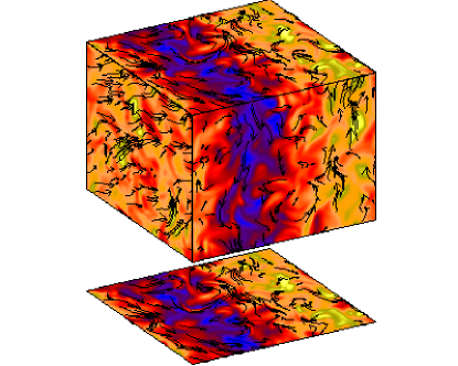
Figure 1: Visualization of the magnetic field in a three-dimensional simulation of helically forced turbulence. The turbulent magnetic field is modulated by a slowly varying component that is force-free.

A helical field of the form (4) is called a Beltrami field. The current density of such a field no longer vanishes; in fact, $\mu_{0}\overline{\bf{J}}=k_{1}\overline{\bf{B}}$, so $\overline{\bf{J}}$ and $\overline{\bf{B}}$ are aligned and

$$\mu_{0}\overline{\bf{J}}\cdot\overline{\bf{B}}=k_{1}\overline{\bf{B}}^{2}=\mbox{const}.$$ (5)

Thus, in the large magnetic Reynolds number limit, Eq. (3) becomes

$$\alpha={\cal O}(\eta_{\rm t}k_{1})\neq 0\quad\mbox{as}\quad R_{\rm m}\rightarrow\infty.$$ (6)

This highlights the great ambiguity in concluding anything about $\alpha$-quenching from oversimplified experiments. [In the discussion above we have assumed that $\alpha_{0}>0$. If $\alpha_{0}<0$, as is the case in B01, then both $\alpha$ and $\overline{\bf{J}}\cdot\overline{\bf{B}}$ are also negative and Eq. (3) is unchanged.]

4 Relation to magnetic helicity

There is a strong connection between $\alpha$-quenching and magnetic helicity conservation. Again, we consider the case of a periodic box, for which it is easy to show that the magnetic helicity

$$H\equiv\int{\bf{A}}\cdot{\bf{B}}\,{\rm d}{}V=\langle{\bf{A}}\cdot{\bf{B}}\rangle V$$ (7)

is perfectly conserved in the limit of infinite magnetic Reynolds number. Here, ${\bf{A}}$ is the magnetic vector potential, so the magnetic field is ${\bf{B}}=\mbox{\boldmath$\nabla$}{}\times{\bf{A}}$, and angular brackets denote volume averages over the full box. If we start with a very weak seed magnetic field, the initial magnetic helicity must also be small and will therefore always remain small if $H$ is conserved. Thus, a large-scale helical field of the form (4) is only compatible with conservation of magnetic helicity if there is an equal amount of magnetic helicity of the opposite sign in the small scales, i.e.

$$\langle{\bf{A}}\cdot{\bf{B}}\rangle\equiv\langle\overline{\bf{A}}\cdot\overline{\bf{B}}\rangle+\langle{\bf{a}}\cdot{\bf{b}}\rangle=0\quad\mbox{(early times)},$$ (8)

where ${\bf{A}}$ and ${\bf{B}}$ have been split up into their mean and fluctuating components,

$${\bf{A}}=\overline{\bf{A}}+{\bf{a}},\quad{\bf{B}}=\overline{\bf{B}}+{\bf{b}}.$$ (9)

Overbars refer to the mean-field obtained by horizontal or azimuthal averaging, for example. Equation (8) is a crucial condition that must be obeyed by any mean-field theory in the large $R_{\rm m}$ limit on time scales shorter than the resistive time scale.

To our knowledge, there have been two approaches to incorporate magnetic helicity conservation into mean-field dynamo theory. One is to express the mean turbulent electromotive force, $\overline{\mbox{\boldmath${\cal E}$}}{}\equiv\overline{{\bf{u}}\times{\bf{b}}}$, as a divergence term (Bhattacharjee & Hameiri 1986, see also Boozer 1993) and the other is to modify the feedback onto the $\alpha$-effect such that Eq. (8) is satisfied on short enough time scales. The latter approach goes back to Kleeorin & Ruzmaikin (1982) and Kleeorin et al. (1995), and has recently been revived by Field & Blackman (2002), Blackman & Brandenburg (2002), and Subramanian (2002). In the following we briefly outline the basic idea.

All we know is that in a closed or periodic domain the magnetic helicity evolves according to

$${{\rm d}{}\over{\rm d}{}t}\langle{\bf{A}}\cdot{\bf{B}}\rangle=-2\eta\mu_{0}\langle{\bf{J}}\cdot{\bf{B}}\rangle,$$ (10)

where $\langle{\bf{A}}\cdot{\bf{B}}\rangle V$ and $\langle{\bf{J}}\cdot{\bf{B}}\rangle V$ are magnetic and current helicities, respectively, and $V$ is the volume. At the same time we have to have some theory for the evolution of the mean magnetic field. The mean-field $\alpha\Omega$ dynamo equations can be written in the form

$${\partial\overline{\bf{B}}\over\partial t}=\mbox{\boldmath$\nabla$}{}\times\left[\overline{\bf{U}}\times\overline{\bf{B}}+\alpha\overline{\bf{B}}-(\eta+\eta_{\rm t})\mu_{0}\overline{\bf{J}}\right].$$ (11)

From this we can construct the evolution equation for the magnetic helicity of the mean field,

$${{\rm d}{}\over{\rm d}{}t}\langle\overline{\bf{A}}\cdot\overline{\bf{B}}\rangle=2\langle\overline{\mbox{\boldmath${\cal E}$}}{}\cdot\overline{\bf{B}}\rangle-2\eta\mu_{0}\langle\overline{\bf{J}}\cdot\overline{\bf{B}}\rangle,$$ (12)

where

$$\overline{\mbox{\boldmath${\cal E}$}}{}=\alpha\overline{\bf{B}}-\eta_{\rm t}\mu_{0}\overline{\bf{J}},$$ (13)

is the mean turbulent electromotive force under the assumption of isotropy. Subtracting Eq. (12) from Eq. (10), we obtain the evolution equation for the magnetic helicity of the fluctuating field,

$${{\rm d}{}\over{\rm d}{}t}\langle{\bf{a}}\cdot{\bf{b}}\rangle=-2\langle\overline{\mbox{\boldmath${\cal E}$}}{}\cdot\overline{\bf{B}}\rangle-2\eta\mu_{0}\langle{\bf{j}}\cdot{\bf{b}}\rangle.$$ (14)

This equation has to be solved simultaneously with the usual mean field equation. At the moment, however, it is not yet fully coupled to the mean field equation. In fact, any kind of coupling, for example of the form

$$\alpha=\alpha\left(\langle{\bf{a}}\cdot{\bf{b}}\rangle,\langle{\bf{j}}\cdot{\bf{b}}\rangle\right)$$ (15)

would suffice. A similar relation could in principle also be applied to the turbulent magnetic diffusivity, $\eta_{\rm t}$. However, in contrast to $\eta_{\rm t}$, $\langle{\bf{a}}\cdot{\bf{b}}\rangle$ and $\langle{\bf{j}}\cdot{\bf{b}}\rangle$ are pseudo-scalars and change sign when $z$ is changed to $-z$. Therefore, only quadratic constructions of the form $\langle{\bf{a}}\cdot{\bf{b}}\rangle^{2}$ and $\langle{\bf{j}}\cdot{\bf{b}}\rangle^{2}$ could, at least in principle, enter into the feedback of $\eta_{\rm t}$.

In an isotropic periodic box we have

$$\langle{\bf{j}}\cdot{\bf{b}}\rangle=k_{\rm f}^{2}\langle{\bf{a}}\cdot{\bf{b}}\rangle,$$ (16)

where $k_{\rm f}$ can be defined by this relation as the typical wavenumber of the fluctuating field. Secondly, we use the relation (Pouquet, Frisch & Léorat 1976)

$$\alpha=-{\textstyle{1\over 3}}\tau\langle\mbox{\boldmath$\omega$}{}\cdot{\bf{u}}\rangle+{\textstyle{1\over 3}}\tau\langle{\bf{j}}\cdot{\bf{b}}\rangle/\rho_{0}$$ (17)

for the residual $\alpha$-effect. This relation describes a fundamental form of $\alpha$-quenching, but there could still be additional feedback onto $\langle\mbox{\boldmath$\omega$}{}\cdot{\bf{u}}\rangle$ and $\langle{\bf{u}}^{2}\rangle$ (Rogachevskii & Kleeorin 2001, Kleeorin et al. 2002), which is ignored here. With these relations, the equation for $\alpha$ becomes explicitly time-dependent,

$${{\rm d}{}\alpha\over{\rm d}{}t}=-2\eta_{\rm t0}k_{\rm f}^{2}\left({\alpha\langle\overline{\bf{B}}^{2}\rangle-\eta_{\rm t}\mu_{0}\langle\overline{\bf{J}}\cdot\overline{\bf{B}}\rangle\over B_{\rm eq}^{2}}+{\alpha-\alpha_{0}\over R_{\rm m}}\right),$$ (18)

where $\alpha_{0}=-{\textstyle{1\over 3}}\tau\langle\mbox{\boldmath$\omega$}{}\cdot{\bf{u}}\rangle$ is the kinematic value of $\alpha$. Here we have expressed the correlation time $\tau$ in terms of $B_{\rm eq}$ using $\eta_{\rm t}={\textstyle{1\over 3}}\tau\langle{\bf{u}}^{2}\rangle$ and $B_{\rm eq}^{2}=\mu_{0}\rho_{0}\langle{\bf{u}}^{2}\rangle$. The full set of equations to be solved comprises thus Eqs (11) and (18).

A detailed analysis of this set of equations was given by Field & Blackman (2002) for the case of the $\alpha^{2}$ dynamo and by Blackman & Brandenburg (2002) for the $\alpha\Omega$ dynamo. The main conclusion is that for large magnetic Reynolds number the large scale magnetic field grows first exponentially such that Eq. (8) is obeyed at all times. This behavior could not have been reproduced with an $\alpha$-effect that is not explicitly time-dependent, such as for example Eq. (1). The exponential growth is then followed by a resistively slow saturation phase, just like in the simulations of B01.

The reason there is this slow saturation phase is that Eq. (8) is incompatible with a steady state, where the right hand side of Eq. (10) must vanish, i.e.

$$\langle{\bf{J}}\cdot{\bf{B}}\rangle\equiv\langle\overline{\bf{J}}\cdot\overline{\bf{B}}\rangle+\langle{\bf{j}}\cdot{\bf{b}}\rangle=0\quad\mbox{(steady state)}.$$ (19)

Since the large scale field is helical, Eq. (5) applies and we have $k_{1}\langle\overline{\bf{B}}^{2}\rangle=k_{\rm f}\langle{\bf{b}}^{2}\rangle$, so the large scale field exceeds the small scale field by a factor $k_{\rm f}/k_{1}$. In the simulations of B01, $\langle\overline{\bf{B}}^{2}\rangle/\langle{\bf{b}}^{2}\rangle$ was about 4, which is indeed close to $k_{\rm f}/k_{1}$=5. In the beginning of the nonlinear regime, Eq. (8) predicts, instead, that $\langle\overline{\bf{B}}^{2}\rangle/\langle{\bf{b}}^{2}\rangle$ equals $k_{1}/k_{\rm f}$, which was 25 times smaller in B01. Figure 2 shows this quantitatively by solving Eqs (11) and (18); see Blackman & Brandenburg (2002).

Figure 2: Evolution of $\langle\overline{\bf{B}}^{2}\rangle$ and $\langle{\bf{b}}^{2}\rangle$ (solid and dashed lines, respectively) in a doubly-logarithmic plot for an $\alpha^{2}$ dynamo with $\eta_{\rm t}=\mbox{const}$ for a case with $k_{\rm f}/k_{1}=10$. Note the abrupt initial saturation after the end of the kinematic exponential growth phase with $\langle\overline{\bf{B}}^{2}\rangle/\langle{\bf{b}}^{2}\rangle\sim 0.1$, followed by a slow saturation phase during which the field increases to its final superequipartition value with $\langle\overline{\bf{B}}^{2}\rangle/\langle{\bf{b}}^{2}\rangle\sim 10$. (Adapted from Blackman & Brandenburg 2002.)

In order to bring the field ratio from 1/5 to 5 we have to remove small scale magnetic helicity resistively. The question is of course what happens if one considers the effects of boundaries (both at the equator and at the outer surface): can boundaries remove small scale magnetic helicity so that the large scale field can saturate at a higher level? This possibility was first brought up by Blackman & Field (2000) and Kleeorin et al. (2000).

5 From closed to open boxes

When the restriction to closed or periodic boxes is relaxed, there can be a flux of magnetic helicity through the surface, so Eq. (10) has then an additional term,

$${{\rm d}{}H\over{\rm d}{}t}=-2\eta\mu_{0}C-Q,$$ (20)

where $H$ and $C$ are magnetic and current helicities, respectively, and $Q$ is the surface integrated magnetic helicity flux. In the presence of open boundaries, however, $H$ and $Q$ are no longer invariant under the gauge transform ${\bf{A}}\rightarrow{\bf{A}}^{\prime}+\mbox{\boldmath$\nabla$}{}\phi$. We use therefore the relative magnetic helicity (Berger & Field 1984, Finn & Antonsen 1985),

$$H=\int_{V}({\bf{A}}+{\bf{A}}_{\rm P})\cdot({\bf{B}}-{\bf{B}}_{\rm P})\,{\rm d}{}V,$$ (21)

where ${\bf{B}}_{\rm P}$ is a potential field used as reference field within the volume $V$, and ${\bf{A}}_{\rm P}$ is its vector potential. Both ${\bf{A}}$ and ${\bf{A}}_{\rm P}$ can have different (arbitrary) gauges.

Following Berger & Field (1984), the reference field obeys the boundary condition ${\bf{B}}_{\rm P}\cdot\hat{\mbox{\boldmath$n$}}{}={\bf{B}}\cdot\hat{\mbox{\boldmath$n$}}{}$, i.e. the normal components of both fields agree on the boundary. In slab geometry, however, the horizontally averaged mean field has to be treated separately and the corresponding reference field is (Brandenburg & Dobler 2001)

$$\overline{\bf{B}}_{\rm P}=\langle\overline{\bf{B}}\rangle=\mbox{const},$$ (22)

so $\overline{\bf{A}}_{\rm P}$ is just a linear function of $z$, $\overline{\bf{A}}_{\rm P}=-\mbox{\boldmath$z$}{}\times\overline{\bf{B}}_{\rm P}$. Brandenburg & Dobler (2001) found from their simulations that most of the magnetic helicity is lost on large scales, where the sign agrees with that of the large scale magnetic helicity. This was a bit disappointing, because one would have hoped that the loss term in Eq. (20) might supersede resistive losses at small scales. That small scale losses can at least in principle enhance the large scale field was shown in subsequent simulations (Brandenburg, Dobler & Subramanian 2002, hereafter BDS; see also Fig. 3). The hope is now that this behavior can eventually be demonstrated using more realistic geometries.

Figure 3: The magnetic energy spectrum for the closed box simulation (solid line) compared with the case where small scale magnetic energy is removed every 100 time steps, corresponding to $\delta t=1.3\times(k_{\rm f}u_{\rm rms})^{-1}$. Note that the large scale magnetic energy (at $k=1$) is enhanced relative to the reference run, whilst the small scale energy is (as expected) reduced.

6 From boxes to spheres

Spherical geometry is necessary to assess more realistically the helicity transfer through equator and outer surfaces, and the relative contributions from rotation, shear, $\alpha$-effect, and turbulent magnetic diffusion. In a recent paper, Berger & Ruzmaikin (2000) estimated that the overall helicity flux at the surface would be around $10^{47}\,{\rm Mx}^{2}$ per 11 year cycle. This value was also confirmed by BDS, who computed numerically solutions of the mean-field dynamo equations in spherical geometry. The relative magnetic helicity for an axisymmetric mean field, $\overline{\bf{B}}=b\vec{\hat{\phi}}+\mbox{\boldmath$\nabla$}{}\times(a\vec{\hat{\phi}})$, takes the very simple form (BDS)

$$H_{\rm N}=2\int_{\rm N}ab\,{\rm d}{}V$$ (23)

where N denotes the volume of the northern hemisphere. The corresponding integrated helicity transfer through the outer surface or the equator is

$$Q_{\rm N}=-2\oint_{\partial V}[(\overline{\mbox{\boldmath${\cal E}$}}{}+\overline{\bf{U}}\times\overline{\bf{B}})\times(a\vec{\hat{\phi}})]\cdot{\rm d}{}{\bf{S}},$$ (24)

where $\overline{\bf{U}}=r\sin\theta\,\Omega\vec{\hat{\phi}}$ is the mean toroidal flow. Note that $Q_{\rm N}=Q_{\rm NS}+Q_{\rm Eq}$, where $Q_{\rm NS}$ is the contribution from the outer surface integral and $Q_{\rm Eq}$ is that from the equatorial plane.

It is remarkable that even in the presence of just uniform rotation alone there is a magnetic helicity flux. For a decaying dipolar magnetic field, the magnetic helicity flux through the equator (from north to south), or, what is the same, into the outer surface of the northern hemispheres, or out of the surface at the southern hemisphere, is $\Phi^{2}$ per rotation, where $\Phi$ is the magnetic flux through one hemisphere.

However, once the field is sustained by a dynamo effect at a constant amplitude, the helicity flux must be balanced by the electromotive force (averaged over one cycle), so

$$\begin{array}[]{lll}Q&=&2\langle\overline{\mbox{\boldmath${\cal E}$}}{}\cdot{\bf{B}}\rangle V-2\eta\mu_{0}\langle\overline{\bf{J}}\cdot\overline{\bf{B}}\rangle V\\ &\equiv&2\alpha\langle\overline{\bf{B}}^{2}\rangle V-2\eta_{\rm T}\mu_{0}\langle\overline{\bf{J}}\cdot\overline{\bf{B}}\rangle V,\end{array}$$ (27)

where $\eta_{\rm T}=\eta+\eta_{\rm t}$ is the total (microscopic plus turbulent) magnetic diffusivity. Assuming that the dynamo is saturated by a reduction of the residual helicity, see Eq. (17), $\alpha_{0}$ and $Q_{\rm N}$ must have opposite signs. This is because saturation requires that ${\rm sgn}\,{}(\alpha_{0})=-{\rm sgn}\,{}(\langle{\bf{j}}\cdot{\bf{b}}\rangle)$, but steady state of Eq. (14) requires that $-{\rm sgn}\,{}(\langle{\bf{j}}\cdot{\bf{b}}\rangle)={\rm sgn}\,{}(\langle\overline{\mbox{\boldmath${\cal E}$}}{}\cdot\overline{\bf{B}}\rangle)$, and ${\rm sgn}\,{}(\langle\overline{\mbox{\boldmath${\cal E}$}}{}\cdot\overline{\bf{B}}\rangle)={\rm sgn}\,{}(Q)$. This can also be seen from a time series of magnetic helicity, and the different terms on the right hand side the ${\rm d}{}H_{\rm N}/{\rm d}{}t$ equation; see Fig. 4.

Thus, if $Q_{\rm N}$ (which denotes only the contributions from the large scale field), is to be identified with the observed negative magnetic helicity flux found on the solar surface (Berger & Ruzmaikin 2000, DeVore 2000, Chae 2000), then we must conclude that $\alpha$ is negative on the northern hemisphere. This scenario, where the main magnetic helicity flux results from the large scales, is consistent with the simulations of BD01. On the other hand, if small scale magnetic helicity is lost preferentially at small scale, and the sign of the small scale magnetic helicity is opposite, then $\alpha$ would in that scenario be positive on the northern hemisphere. This would be consistent with the observed negative sign of current helicity on the northern hemisphere (Seehafer 1990, Pevtsov et al. 1995, Bao et al. 1999, Pevtsov & Latushko 2000), which is plausibly a proxy of small scale magnetic helicity.

Figure 4: Time series of the nondimensional ratio $H/2\mu_{0}\langle M\rangle R$ compared with magnetic energy (in nondimensional units and scaled by 1/20). Magnetic helicity is mostly positive in the northern hemisphere. The helicity production, $S$, from $\alpha$-effect and turbulent magnetic diffusion is mostly positive and balanced here by a mostly positive magnetic helicity flux (dashed and dotted lines refer to the contributions from the angular velocity and the $\alpha$-effect, respectively).

Within the framework of mean-field $\alpha\Omega$ dynamo theory, a negative $\alpha$ in the nothern hemisphere would explain the observed migration of the sunspot belts, so one would not need to resort to meridional circulation driving the dynamo wave. However, there is as yet no well established mechanism to explain a negative $\alpha$ (except perhaps magnetic buoyancy with shear; cf. Brandenburg 1998).

Observations do not seem to be able to tell us which of the two scenarios is right, because it is difficult to tell whether the observed magnetic helicity flux is from large or small scale fields. If the observed magnetic helicity flux is from small scale, one might wonder why one cannot see the magnetic helicity flux from the large scales. On the other hand, if the observed magnetic helicity flux is actually already due to the large scales, one might expect to see small scale magnetic helicity fluxes at higher resolution in the future.

7 Conclusions

Magnetic helicity seems to play a much more prominent role than what has been anticipated until recently. It has become clear that $\alpha$ must satisfy an explicitly time-dependent equation. The dynamical $\alpha$-quenching theory has significant predictive power: it describes the different quenching behaviors for helical and nonhelical fields, the value of the magnetic Reynolds number is explicitly incorporated, and the magnetic helicity equation is satisfied exactly at all times. So far, no departures between this theory and the simulations have been found. A major restriction of the theory in its present form is however the inability to handle cases with spatially nonuniform $\alpha$-effect.

Id: paper.tex,v 1.16 2002/06/11 15:35:54 dobler Exp