Future supernovae data and quintessence models

Abstract

The possibility to unambiguously determine the equation-of-state of the cosmic dark energy with existing and future supernovae data is investigated. We consider four evolution laws for this equation-of-state corresponding to four quintessential models, i.e. i) a cosmological constant, ii) a general barotropic fluid, iii) a perfect fluid with a linear equation-of-state and iv) a more physical model based on a pseudo-Nambu-Goldstone boson field. We explicitly show the degeneracies present not only within each model but also between the different models : they are caused by the multi-integral relation between the equation-of-state of dark energy and the luminosity distance. Present supernova observations are analysed using a standard $\chi^{2}$ method and the minimal $\chi^{2}$ values obtained for each model are compared. We confirm the difficulty to discriminate between these models using present SNeIa data only. By means of simulations, we then show that future SNAP observations will not remove all the degeneracies. For example, wrong estimations of $\Omega_{m}$ with a good value of $\chi^{2}_{min}$ could be found if the right cosmological model is not used to fit the data. We finally give some probabilities to obtain unambiguous results, free from degeneracies. In particular, the probability to confuse a cosmological constant with a true barotropic fluid with an equation-of-state different from $-1$ is shown to be $95\,\%$ at a $2\,\sigma$ level.

1 Introduction

Present supernovae data strongly support cosmological models containing a perfect fluid with a negative pressure (Riess et al. 1998, Perlmutter et al. 1999). The oldest and most studied candidate for this fluid is the cosmological constant, which acts like a perfect fluid whose equation-of-state (hereafter, EOS) is $w\equiv p\,/\,\rho=-1$, where $p$ is the fluid pressure and $\rho$ its density. But the vacuum energy density associated with the cosmological constant is 60-120 orders of magnitude smaller than its natural value derived from quantum field theories. This discrepancy is known as the cosmological constant problem (Abbott 1988, Weinberg 1989, Carroll et al. 1992, Sahni & Starobinsky 2000) and has led theorists to find alternative dark energy candidates with a present negative pressure. The simplest models are based on a generalisation of the cosmological constant, e.g. a barotropic fluid ($w(z)=w_{0}=$ constant $<1$ ; González-Díaz 2000, Di Pietro & Demaret 2001) or a homogeneous fluid for which $w$ is a linear function of $z$ ($w(z)=w_{0}+w_{1}\,z$ with $w_{0}$ and $w_{1}$ constant ; Goliath et al. 2001, Maor et al. 2001, 2002).

These models are interesting because they are described by simple field equations. However, they suffer from a lack of physical justification. Other models with a more general EOS and stronger physical interpretation have been proposed (Peebles & Ratra 1988, Ratra & Peebles 1988, Wetterich 1988, Ferreira & Joyce 1998, Steinhardt et al. 1999). The most popular ones are based on a dynamical quintessential component represented by a minimally coupled scalar field evolving in a potential. Mathematically, such a quintessence fluid can be described by an EOS $w$ function of the redshift $z$ ($-1\leq w(z)\leq 1$). Among these quintessence models, we shall consider the one which assumes the existence of an ultra-light pseudo-Nambu Goldstone boson (PNGB) field relaxing to its vacuum state (Frieman & Waga 1998, Waga & Frieman 2000, Ng & Wiltshire 2001a). From the quantum viewpoint, the PNGB models are the simplest way to introduce a naturally ultra-light scalar field able to reproduce the cosmological observations (Frieman et al. 1992, 1995). Moreover PNGB models provide an interesting theoretical framework to any spontaneous symmetry breaking which could justify the neutrino mass found in the Mikheyev-Smirnov-Wolfenstein solution to the solar neutrino problem (Wolfenstein 1979, Mikheyev & Smirnov 1985).

In summary, many theoretical models describing a cosmological fluid with negative pressure have been proposed : some are designed to be mathematically simple while others rely on a more physical justification. The first aim of this paper is to put in evidence the strong degeneracies existing between the luminosity distance predicted by four quintessence models : a cosmological constant, a general barotropic fluid, a fluid with a linear equation-of-state and a more physical model based on a pseudo-Nambu-Goldstone boson field. Second, we shall determine the constraints on those models coming from the present observations of type Ia supernovae (hereafter, SNeIa) and confirm the need for more data to discriminate between them. This may be fulfilled by the proposed SNAP satellite (SuperNova/Acceleration Probe ; see SNAP URL). The main objective of this instrument is to detect a very large number of supernovae up to a redshift of $1.7$, in order to yield a more precise determination of the cosmological parameters and therefore to provide information on the nature of dark energy. The third objective of this paper is to analyse, by means of simulated data, how well future SNAP observations alone will be able to break the degeneracies that we put in evidence.

Several authors have already studied the feasibility of SNAP to determine the properties of the dark energy. Depending on the method used for reconstructing the cosmological model, their conclusions are quite different : some authors are optimistic regarding the possible determination of the EOS of the dark energy using SNeIa (Huterer & Turner 1999, Nakaruma & Chiba 1999, Saini et al 2000, Chiba & Nakaruma 2000, Weller & Albrecht 2001, 2002) while others are more cautious (Barger & Marfatia 2001, Astier 2001, Maor et al. 2001, 2002, Gerke & Efstathiou 2002). Most of these discrepancies can be traced back to the differences in initial assumptions, prior knowledge, … used for the reconstruction of the cosmological model (Goliath 2001). Usually, optimistic conclusions result from strong assumptions, such as an accurate knowledge of $\Omega_{m}$.

The structure of the paper is as follows. In Section 2, we present the field equations describing the four cosmological models we have considered. In Section 3, we explicitly display the degeneracies between the luminosity distances predicted by these four models. The constraints brought by present SNeIa data on the parameters of each model are presented in Section 4. In Section 5, we explore the ability of SNAP to break the degeneracies and so to discriminate among these models. Finally, we summarize our work and give some conclusions in Section 6.

2 Quintessence models : theoretical framework

The field equations of a Friedmann-Lemaître-Robertson-Walker spacetime filled with two non-interacting fluids, a pressureless fluid (matter - $\Omega_{m}$) and a spatially homogeneous scalar field $\phi$ in a potential $V(\phi)$ (quintessence - $\Omega_{x}$), can be written as

$$\displaystyle\frac{H^{2}(z)}{H_{0}^{2}} = \Omega_{m}\,(1+z)^{3}+\Omega_{k}\,(1+z)^{2}+\Omega_{x}\,g(z)$$ (1)

$$\displaystyle\rho^{\prime}_{x}(z) = -\,3\,[\rho_{x}(z)+p_{x}(z)]\,H(z)$$ (2)

$$= \,-\,3\,[1+w(z)]\,\rho_{x}(z)\,H(z),$$

where the prime denotes the time derivative, $H(z)$, the Hubble parameter, $\Omega_{k}$, the curvature parameter ($\Omega_{k}=1-\Omega_{m}-\Omega_{x}$) and where

$$\displaystyle\kappa\,\rho_{x}(z) \equiv \displaystyle\frac{1}{2}\,\phi^{\prime 2}(z)+\,V(\phi(z)),$$ (3)

$$\displaystyle\kappa\,p_{x}(z) \equiv \displaystyle\frac{1}{2}\,\phi^{\prime 2}(z)-\,V(\phi(z)),$$ (4)

$$w(z) \equiv \displaystyle\frac{\,p_{x}(z)}{\,\rho_{x}(z)},$$ (5)

$$g(z) \equiv \displaystyle\frac{\rho_{x}(z)}{\rho_{x,0}}$$ (6)

$$= \displaystyle(1+z)^{3}\,\,\exp\left[\int_{0}^{z}{3\,w(z^{\prime})\,d\,\ln(1+z^{\prime})}\right],$$ (7)

with $\kappa=8\,\pi\,G$.

When the scalar field acts like a fluid with a linear EOS in $z$, i.e. $w(z)=w_{0}+w_{1}\,z$, equation (7) becomes $g(z)=e^{3\,w_{1}\,z}\,\,(1+z)^{3\,(1+w_{0}-w_{1})}$ and the Friedmann equation given by (1) can be written as

$$H^{2}(z) = \displaystyle H_{0}^{2}\,\left\{(1+z)^{2}\left[\Omega_{m}\,z\,+1\right]\right.$$ (8)

$$+ \displaystyle\left.\Omega_{x}(1+z)^{2}\left[e^{3w_{1}z}\,(1+z)^{1+3(w_{0}-w_{1})}-1\right]\right\},$$

where the relation between the density parameters has been used, i.e. $\Omega_{k}=1-\Omega_{m}-\Omega_{x}$.

The luminosity distance $d_{L}(z)$ to an object at redshift $z$ is such that

$$\displaystyle D_{L}^{th}(z) \equiv \displaystyle\frac{d_{L}(z)\,H_{0}}{c}$$ (9)

$$\equiv \displaystyle\frac{(1+z)}{\sqrt{\mid\Omega_{k}\mid}}\,\,\,\,S\left(\int_{0}^{z}\frac{\sqrt{\mid\Omega_{k}\mid}\,\,H_{0}\,\,dz^{\prime}}{H(z^{\prime})}\right)$$ (10)

with $S(x)=\sin(x),x,\sinh(x)$ for respectively a spatially closed, flat and open universe. Note that $d_{L}$ is the luminosity distance whereas $D^{th}_{L}$ is a dimensionless quantity. For $d_{L}$ in units of Mpc, the apparent magnitude can be expressed in terms of $D_{L}^{th}$ as follows

$$m_{B}=5\,\log(D_{L}^{th})+\bar{M}_{B}$$ (11)

where $\bar{M}_{B}$ is the magnitude zero point in the $B$ band defined by

$$\bar{M}_{B}\equiv M_{B}-5\,\log[H_{0}\,/\,c\,]+25$$ (12)

with $M_{B}$, the absolute magnitude of the SNeIa.

Hereafter, we focus on three types of models containing a scalar fluid with a linear EOS (cf. also models A, B and C in Table 1) :

1. Model A : a scalar field still acting as a cosmological constant with no constraint on the geometry of the universe, i. e. a FLRW model,

2. Model B : a scalar fluid with a constant EOS in a spatially flat universe,

3. Model C : a scalar fluid with a linear EOS in a spatially flat universe.

These models are mathematically the simplest ones but they have no satisfactory physical interpretation. So we shall also consider a fourth quintessence model, based on physical arguments. This model is constructed with an ultra-light pseudo-Nambu-Goldstone boson (PNGB) field (Frieman & Waga 1998, Waga & Frieman 2000, Ng & Wiltshire 2001a, 2001b). In quantum field theory, a Nambu-Goldstone boson field is generated when a global symmetry is spontaneously broken. Moreover, if this symmetry is explicitly broken, the Nambu-Goldstone boson acquires a mass and becomes a pseudo-Nambu-Goldstone boson. A quintessence model based on a PNGB field can be described by the field equations (1)-(7) with the following periodic potential (Frieman et al. 1992, 1995) :

$$V(\phi)=M^{4}\,\left(\cos\left[\phi\,/\,f\right]+1\right)$$ (13)

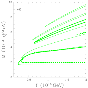
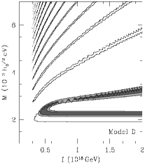
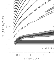
where $M$ and $f$ are the two mass scales, i.e. $f$ is the spontaneous- and $M$ is the explicit symmetry breaking scale. For such a model, the field equations (1)-(7) have no analytical solution. Therefore, the behavior of the functions $g(z)$ and $H(z)$ can only be derived from a numerical integration. We take as initial conditions $\phi^{\prime}_{i}=0$ and $\phi_{i}=10^{-2}\,m_{Pl}$ where $m_{Pl}$ is the reduced Planck mass (see justification below). Assuming again a spatially flat universe, we are left with a model depending on only two parameters, $M$ and $f$. This model is referred to as “Model D ” (cf. also Table 1) and its most important properties are summarized in Figures 1 and 2. Because of the Hubble damping, the PNGB field is initially frozen near the top of its potential ($\,\phi_{i}^{\prime}\sim 0\,$ and $\,\phi_{i}\ll\,f$) and therefore acts as a cosmological constant, so that $w(z\gg 1)\approx-1$. When the universe temperature becomes less than the PNGB mass, i.e. $\,m_{\phi}=M^{2}\,/\,f\,$, the field starts to slowly roll down the potential. The minimum of the potential is reached asymptotically, after a large number of coherent oscillations about it. This second phase corresponds to a scalar component which behaves on average as nonrelativistic matter. It means that model D looks initially like model A with $\Omega_{k}=0$ and asymptotically like an Einstein-de Sitter universe. The larger the quintessence mass, the sooner the asymptotic state is reached. If the scalar field evolution starts before its energy density becomes dominant, the PNGB field will never be relevant for the universe dynamics (see Figure 1A). However, if the dynamical phase of the scalar field begins when the vacuum energy associated with the PNGB field is already dominant, then the scalar energy density may dominate today the cosmic density of the universe and provide a non-negligible dark energy component (see Figure 1B).

Name	Constraints	Parameters
Model A	$w_{0}=\,-\,1$ and $w_{1}=0$	$\Omega_{m}$, $\Omega_{x}$
Model B	$\Omega_{m}+\Omega_{x}=1$ and $w_{1}=0$	$\Omega_{m}$, $w_{0}$
Model C	$\Omega_{m}+\Omega_{x}=1$ and $\Omega_{m}=0.3$	$w_{0}$, $w_{1}$
Model D	$\Omega_{m}+\Omega_{x}=1$ and	$M$, $f$
	$V(\phi)=M^{4}\,(\cos[\phi\,/\,f]+1)$

Table 1: Characteristics of the four theoretical models considered in this paper.

Figure 1: Behavior of $\rho_{\phi}$ (thick) and $\rho_{m}$ (thin), in units of the present critical density, when the quintessence component is a PNGB field. In the small boxes, the corresponding behavior of $w_{\phi}$ is given. Negative redshifts are associated with the future of the universe. For A : $\,M=1.4\times 10^{-3}h_{0}^{1/2}$ eV and $\,f=3\times 10^{17}$ GeV. For B : $\,M=4\times 10^{-3}h_{0}^{1/2}$ eV and $\,f=5\times 10^{17}$ GeV.

Figure 2: $M-f$ diagram for the PNGB model. The shaded areas represent the parameter regions where the universe is presently accelerating whereas the solid lines are the curves of equal $\Omega_{m}$ with $\Omega_{m}=0.8$, $0.6$, $0.4$, $0.2$, from left to right.

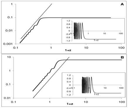
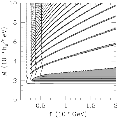
Figure 2 shows examples of curves of equal $\Omega_{m}$ in an $M-f$ diagram. The shaded area represents the parameter regions in which the expansion is accelerating today. In these regions, the kinetic energy of the PNGB field is small compared to its potential. This occurs either when the scalar field is still frozen (the lowest and largest shaded band) or when its first derivative changes sign, i.e. when $\phi^{\prime}\sim 0$ (the thin shaded bands). Regions outside these shaded areas correspond to models where the scalar field is presently near the minimum of its potential (for more details on PNGB models, see Frieman et al. 1992, 1995, Frieman & Waga 1998, Waga & Frieman 2000, Ng & Wiltshire 2001a).

Figure 3: Curves of equal luminosity distance in the framework of the four cosmological models considered in this paper. (a) Model A : the dashed curves represent the set of values for $(\Omega_{m},\Omega_{\Lambda})$ such that $D_{L}(z_{i};\Omega_{m},\Omega_{\Lambda})=D_{L}(z_{i};0,0)$, with $z_{i}=0.05,0.4,0.8,1.0,1.2,1.4$. Similarly, the solid curves show the set of values for $(\Omega_{m},\Omega_{\Lambda})$ such that $D_{L}(z_{i};\Omega_{m},\Omega_{\Lambda})=D_{L}(z_{i};0,-1)$, with $z_{i}=0.05,0.4,0.8,1.0,1.2,1.4$. (b) Model B : the curves represent the set of values for $(\Omega_{m},w_{0})$ such that $D_{L}(z_{i};\Omega_{m},w_{0})=D_{L}(z_{i};0.7,-0.5)$ (top) and $D_{L}(z_{i};\Omega_{m},w_{0})=D_{L}(z_{i};0.3,-0.7)$ (bottom), with $z_{i}=0.05,0.4,0.8,1,1.2,1.4$. (c) Model C : the curves represent the set of values for $(w_{0},w_{1})$ such that $D_{L}(z_{i};w_{0},w_{1})=D_{L}(z_{i};-0.3,0.2)$ (top) and $D_{L}(z_{i};w_{0},w_{1})=D_{L}(z_{i};-0.7,-0.5)$ (bottom), with $z_{i}=0.05,0.4,0.8,1,1.2$ and $1.4$. (d) Model D : curves show the set of values of $(f,M)$ such that $D_{L}(z_{i};f,M)=D_{L}(z_{i};0.5,3)$ with $z_{i}=0.4$ (thin), $0.8$ (thick) and $1.2$ (dashed).

3 Degeneracies between the quintessence models

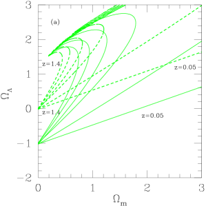
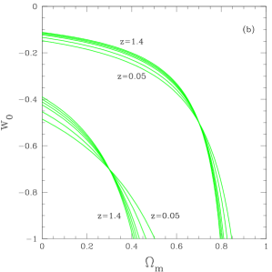
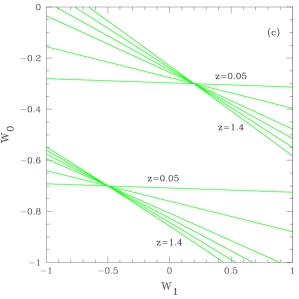
Since the SNeIa apparent magnitudes are sensitive to the luminosity distance and since the latter is related to the model parameters through a multiple integral (see eq. (10) with (1) and (7)), it is quite natural to expect some degeneracies between the different models. This is even true within a given cosmological model. Indeed, Figure 3 shows curves of equal luminosity distance for different redshifts, in the parameter spaces of the four models. For each model, the curve shape varies with the given redshift. The curves intersect in one point in models A, B and C and this lifts the degeneracy. But in model D, the contours could remain close to each other, making more difficult a clear estimation of the cosmological parameters.

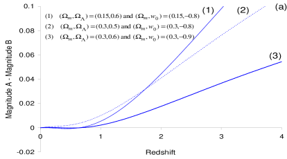
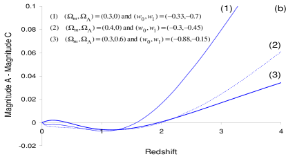
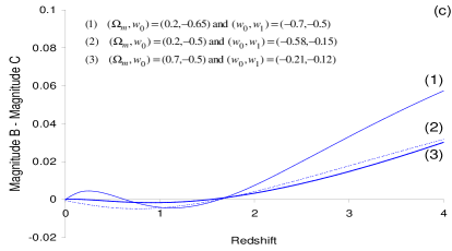
The situation is even worse when comparing the different models. Indeed, Figure 4 shows expected magnitude differences between different models, versus redshift. Specific choices of parameters of either model A, B, C or D can yield magnitude differences less than 0.04 mag all the way to $z=2$. These are really small compared to the 0.15 mag intrinsic dispersion of the SNeIa maximum luminosity. In other words, as already mentionned by Maor et al. (2001, 2002), different function $w(z)$ can approximatively lead to the same $d_{L}(z)$ relation. A large number of SNeIa observations with very good photometry are needed in order to break these degeneracies. At this point, data at large redshifts ($z>2$) could be more than useful.

Figure 4: Comparison between the magnitudes predicted by various models A and B (a), models A and C (b), models B and C (c) and models C and D (d).

Figure 5: Curves in the parameter space of model B such that $D_{L}(z_{i};\Omega_{m},w_{0})$ built with this model is equal to $D_{L}(z_{i};w_{0}=-0.7,w_{1}=-0.5)$ (left) and to $D_{L}(z_{i};w_{0}=-0.3,w_{1}=0.2)$ (right) derived from model C, for $z_{i}=0.05,0.4,0.8,1,1.2,1.4,1.7,3$. The presence of degeneracies is revealed by the fact that the different curves cross each other over a very small area in the parameter space. The curves corresponding to $z=3$ (dotted) indicate that the degeneracy could break at very large redshifts.

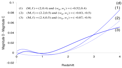Figure 5 illustrates that estimates of the cosmological parameters can simply be erroneous if a wrong cosmological model is chosen for the analysis. Here are the different steps followed to draw this plot :

1. We chose some values of the parameters describing the model C, i.e. $(w_{0},w_{1})=(-0.7,-0.5)$.

2. The luminosity distance predicted by model C at $z=0.05$ were numerically computed.

3. We then searched the parameters $(\Omega_{m},w_{0})$ for which model B predicts the same luminosity distance at $z=0.05$. We plotted the curve of equal luminosity distance obtained in the parameter space of model B.

4. We repeated the two previous steps for different values of $z$, i.e. $z=0.4,0.8,1,1.2,1.4,1.7,3$, and plotted the $6$ corresponding curves.

5. The four previous operations were repeated with a second set of parameters for the model C, i.e. $(w_{0},w_{1})=(-0.3,0.2)$.

Keeping in mind that models C are defined with $\Omega_{m}=0.3$, Figure 5 clearly shows that the value of $\Omega_{m}$ would not be properly recovered by fitting model B on the data. Indeed, the first set of curves ( correspondong to $(w_{0},w_{1})=(-0.7,-0.5)$ in model C) all cross over a very small area characterized by $(\Omega_{m},w_{0})\approx(0.15,-0.6)$. Similarly, the second set of curves (corresponding to $(w_{0},w_{1})=(-0.3,0.2)$ in model C) would lead to an estimate of $(\Omega_{m},w_{0})\approx(0.65,-0.6)$ if the data analysis was carried out with model B. These results mean that the same data can lead to different estimates of $\Omega_{m}$ and $w_{0}$, depending on the cosmological model used for the data analysis. In other words, the role of the derivative of the dark energy EOS on the luminosity distance can be played by a matter density parameter in models with a constant EOS : a model with a fixed $\Omega_{m}$ containing a fluid described by a negative (positive) $w_{1}$ can be mistaken with a model described by a smaller (larger) $\Omega_{m}$ containing a barotropic fluid (see also Figure 12). Note that the dotted curve corresponding to $z=3$ shows degeneracy breaking at very large redshifts (see also Figure 4).

4 Quintessence models and present SNeIa data

We used the published data of Perlmutter et al. (1999; P99 hereafter), which consist of a sample containing 60 SNeIa, to determine the constraints that we have today on the parameters describing the four models introduced in Section 2. As it has been noted in P99, four of these supernovae are “outliers”. So we excluded them and considered a sample of only 56 SNeIa. We analysed these data with a standard $\chi^{2}$ method, i.e. by minimizing the value of $\chi^{2}$ defined by

$$\chi^{2}=\sum_{i=1}^{56}{\frac{\left[m^{th}_{B}(z_{i};\theta_{1},\theta_{2},\bar{M}_{B})-m_{B,i}^{data}\right]^{2}}{\sigma_{i}^{2}}},$$ (14)

where $m^{th}_{B}$ (resp. $m^{data}_{B}$) are the effective apparent magnitudes (i. e. the observed magnitudes corrected by the lightcurve width-luminosity relation, the Galactic extinction, the K-correction and the cross-filter calibration) predicted by the model (resp. given by the data). $\sigma_{i}$ are the uncertainties on the data and $\theta_{1}$ et $\theta_{2}$ are the two parameters of the theoretical model (cf. Table 1).

Figure 6: $68.3\%$ (dark) and $95.4\%$ (light) confidence contours obtained by analysing P99 data with each model. Solid curves separate universes which are presently decelerating from those which are presently accelerating. The four plots on the left (resp. on the right) are obtained with $\bar{M}_{B}=24$ (resp. with no prior constraints on $\bar{M}_{B}$).

Concerning $\bar{M}_{B}$, we adopted two different approaches. We first assumed that $\bar{M}_{B}$ was exactly known and equal to $24$, all uncertainties on this parameter being neglected. In the second approach, we assumed no prior constraint on $\bar{M}_{B}$, which is just an unknown constant with a value between $-\infty$ and $+\infty$. In this case, we integrated the probabilities on $\bar{M}_{B}$ and therefore worked with a $\bar{\chi}^{2}$ defined by

$$\bar{\chi}^{2}=-2\,\ln\left(\int^{+\infty}_{-\infty}{e^{-\chi^{2}/2}\,d\bar{M}_{B}}\right)=A-\frac{B^{2}}{C}+\ln\left(\frac{C}{2\pi}\right),$$ (15)

where

$$A = \sum_{i=1}^{56}{\frac{\left(m_{B,i}^{data}-5\,\log[D_{L}^{th}]\right)^{2}}{\sigma_{i}^{2}}},$$ (16)

$$B = \displaystyle\sum_{i=1}^{56}{\frac{m_{B,i}^{data}-5\,\log[D_{L}^{th}]}{\sigma_{i}^{2}}},$$ (17)

$$C = \displaystyle\sum_{i=1}^{56}{\frac{1}{\sigma_{i}^{2}}}.$$ (18)

Note that a uniform distribution of the probabilities on a relatively small interval, i.e. $\bar{M}_{B}=24\pm 0.2$, gives the same results as a uniform distribution between $-\infty$ and $+\infty$.

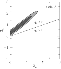
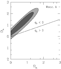
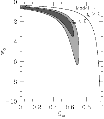
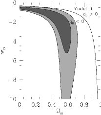
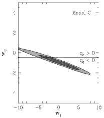
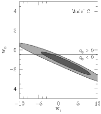
We analysed the sample of 56 SNeIa given in P99 using as framework the four theoretical models discussed in Section 2 and for two opposite assumptions on $\bar{M}_{B}$. The probability contours are shown in Figure 6. Table 2 lists the best fit values of the parameters together with the $\chi^{2}_{\rm min}$ and $\chi^{2}_{\rm min}/$DOF (DOF : Degree of freedom).

The results obtained using model A are in agreement with those found in the literature (P99). Small differences may be related to the fact that we used data already corrected for the stretch-factor whereas P99 integrate on this parameter. However, these differences are not relevant in view of our objectives. Results concerning model B show that present data agree with a baroropic fluid characterized by $w_{0}<-0.4$ at the $2\,\sigma$ level. An important remark has to be made concerning models B and C : Figure 6 indicates that the data favour unphysical regions where $w_{0}<-1$ (see also Caldwell 2002). Note that if we restrict ourselves to models with $w_{0}\geq-1$, the best fit positions, characterized by $(\Omega_{m},w_{0})=(0.3,-1)$ in model B and by $(w_{0},w_{1})=(-1,0.6)$ in model C, are associated to $\chi^{2}_{\rm min}$ values only marginally different from those obtained when $w_{0}<-1$ ($\Delta\chi^{2}_{\rm min}<0.1$). The fact that the true minimum is located in a unphysical region is something that has to be strongly considered in the future because, if confirmed, it can rule out these models.

Model	$\chi^{2}_{\rm min}$	$\chi^{2}_{\rm min}/$DOF	$\theta_{1}$	$\theta_{2}$
$A$	$62.1$	$1.15$	$\Omega_{m}=0.6$	$\Omega_{\Lambda}=0.9$
$B$	$62.2$	$1.15$	$\Omega_{m}=0.41$	$w_{0}=-1.2$
$C$	$62.2$	$1.15$	$w_{0}=-1.1$	$w_{1}=0.9$
$D$	$62.2$	$1.15$	$M=2.3$	$f=0.5$

Model	$\bar{\chi}^{2}_{\rm min}$	$\bar{\chi}^{2}_{\rm min}/$DOF	$\theta_{1}$	$\theta_{2}$
$A$	$66.8$	$1.26$	$\Omega_{m}=0.8$	$\Omega_{\Lambda}=1.3$
$B$	$67.4$	$1.27$	$\Omega_{m}=0.46$	$w_{0}=-1.6$
$C$	$67.3$	$1.27$	$w_{0}=-1.4$	$w_{1}=2.3$
$D$	$67.4$	$1.27$	$M=2.3$	$f=0.5$

Table 2: Minimum values of $\chi^{2}$ and $\bar{\chi}^{2}$ obtained when the analysis of the existing data is carried out on each of the four quintessence models. The upper table assumes $\bar{M}_{B}=24$ whereas the lower one assumes no prior constraints on $\bar{M}_{B}$.

The constraints for model D select two sorts of regions (Figure 6 ; see also Ng & Wiltshire 2001b) : one where the scalar field is still frozen (lower horizontal band) and another where its evolution has just begun (upper oblique band). Note that these contours are not closed : the larger the $f$, the more the two branches are separated. A small part of the $2\,\sigma$ contours also appears on the second plot of model D, selecting a region with $M\sim 6\times 10^{-3}\,h_{0}^{1/2}$ eV. If we adopt the point-of-view that the PNGB field of model D is related to the resolution of the solar neutrino problem, then the value of $M$ gives an estimate of the neutrino mass (Frieman et al. 1992, 1995). The last two plots of Figure 6 show that at least one neutrino species has a mass of : $\sim 2\times 10^{-3}\,h_{0}^{1/2}$ eV, if the PNGB field is still frozen, $\sim 3\times 10^{-3}\,h_{0}^{1/2}$ eV, if the field is just starting to evolve or $\sim 6\times 10^{-3}\,h_{0}^{1/2}$ eV ($2\,\sigma$ region on the second plot), if the field has already passed one time through the potential minimum. These estimates are indeed similar to the ones found by SuperKamiokande and SNO (Sudbury Neutrino Observatory) for the neutrino mass squared differences, i.e. $\delta m_{23}^{2}=(1.6-3.9)\times 10^{-3}$ eV² (Fukuda et al. 1998) and $\delta m_{12}^{2}=(0.3-3.5)\times 10^{-4}$ eV² (Choubey et al. 2002 and references therein). This may be only a numerical coincidence… or it may comfort us in the resolution of the neutrino problem through a Goldstone mechanism.

Note that contours where $M\sim 3\times 10^{-3}\,h_{0}^{1/2}$ eV or $6\times 10^{-3}\,h_{0}^{1/2}$ eV are associated to small values of $\Omega_{m}$ ($\ll 0.1$ ; see Figure 2) which are inconsistent with observations (Peebles & Ratra 2002). The value of $f$ is only poorly constrained by the present data. This is because $f$ becomes an important parameter for the cosmological model only when the scalar field evolves in its potential, not when it is frozen or just starting to move.

As it can be seen on Figure 6, in some cases, present data can also favour a decelerating universe, even at $1\,\sigma$ level. An important remark has to be made concerning the $\chi^{2}_{\rm min}$ values presented in Table 2 : in both approaches for $\bar{M}_{B}$, the four values of $\chi^{2}_{\rm min}$ are very close to each other. In particular, the differences between them are much less than the $1\,\sigma$ interval ($\Delta\chi^{2}=2.3$). Therefore, as expected, the present data are not sufficient to discriminate between these four quintessence models even at the $1\,\sigma$ confidence level.

5 Quintessence models and future SNeIa observational data

The analysis of the present SNeIa data discussed in the previous section clearly showed that more observations are needed to clearly determine the nature of the dark energy. Such data could be provided by the proposed SNAP (“SuperNova/Acceleration Probe”) mission (see SNAP URL). SNAP, if accepted, will be a two-meter space telescope dedicated to the discovery and observation of SNeIa with redshifts in the range $0<z<1.7$. This instrument should perform photometry and spectroscopy of more than 2000 SNeIa per year. The aim of this section is to investigate which values of the parameters (chosen by Mother Nature), future SNAP observations will be able to discriminate. The analysis will also reveal degeneracies between individual parameters of the different models.

We have first generated mock SNAP data by successively assuming that model A, B, C or D was the true one, and under the ideal hypothesis that $\bar{M}_{B}$ was exactly known. For each model, we have selected 100 couples of parameters restricted to physical regions surrounding contours given on Figure 6 (see Table 3). This is why the $w_{0}$ parameter has been limited to $[-1;0]$. The $w_{1}$ parameter of model C has been limited to the interval $[-1;1]$, in order to avoid large absolute values of the EOS at $z\geq 1$. The parametrization adopted to generate data from model D means that we restricted ourselves to universes different from an Einstein-de Sitter one ($M<5$) or to universes characterized by $\Omega_{m}<0.6$ ($f>0.4$ or $M>2$) (cf. Figure 2).

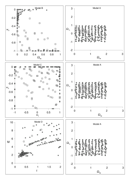
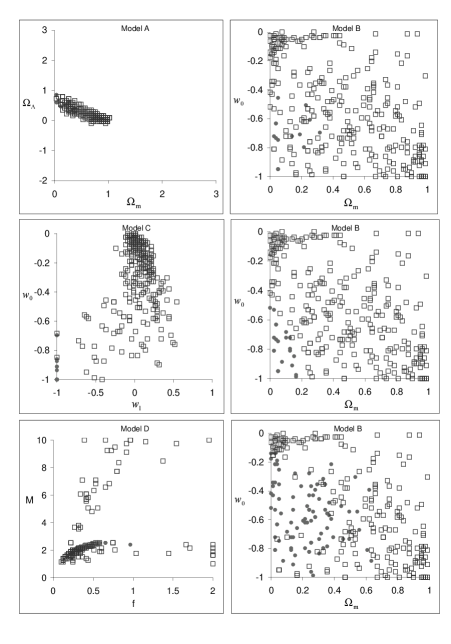
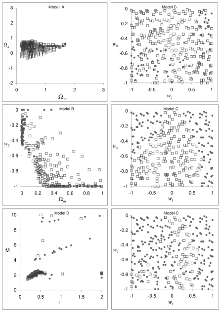
Then, for each value of the parameters, we have generated three samples. For each of them we have computed the magnitude of 2100 SNeIa, with 2000 uniformly distributed in the redshift interval $z\in[0;1.2]$ and 100 in the redshift interval $z\in[1.2;1.7]$. Gaussian errors on the magnitude have been added with a standard deviation of 0.15 mag, reflecting only the intrinsic spread of the SNeIa maximum luminosity (see SNAP URL). So for each of the four models, we are left with $3\times 100$ sets of SNAP data, for which we know the parent model. Then, each sample has been independently fitted with the four models. The results are presented in Figures 7, 9, 11 and 13 where the parent is model A, B, C, D respectively. The parent model is in the right column and is successively compared to the other models. The squared symbols select the value of the parameters for which the two models are degenerated at the $2\,\sigma$ level, i.e. for which $\Delta\,\chi^{2}_{\rm min}<6.17$, whereas the filled dots represent the parameters for which $\Delta\,\chi^{2}_{\rm min}>6.17$ . Since we simulated noisy data, fitting the true model may not yield the exact value of the parameters. That is why the sets of models do not reproduce a regular grid in the right column of Figures 7, 9, 11 and 13. Moreover, different best fit positions can be associated to several simulations.

Model	Values used for generate samples
A	$\Omega_{m,i}=0.1-(1-i)\,/\,5$
	$\Omega_{\Lambda,j}=-0.9\,+0.2\,(j-1)$
B	$\Omega_{m,i}=0.05+(i-1)\,/\,10$
	$w_{0,j}=-0.05-(j-1)\,/\,10$
C	$w_{0,i}=-0.05+(1-i)\,/\,10$
	$w_{1,j}=-0.95\,(2\,j-11)\,/\,9$
D	$f_{i}=0.4+1.6\,(i-1)\,/\,9\,$
	$M_{j}=2+(j-1)\,/\,3\,$

Table 3: Values of the parameters used for the SNAP data simulations ($i,j=1,...,10$).

Figure 7: Positions of the $\chi^{2}_{\rm min}$ in the four models of the $300$ simulated data samples generated with model A. The filled circles (resp. empty squares) correspond to $\Delta\,\chi^{2}_{\rm min,X-A}>6.17$ (resp. $\Delta\,\chi^{2}_{\rm min,X-A}<6.17$) for $X=B,C,D$.

Figure 8: Correlations between individual parameters of model A and model C (when $\Delta\chi^{2}_{\rm min}<6.17$). Upper plot - between $\Omega_{m}-\Omega_{\Lambda}$ of the correct model A and $w_{0}$ of the wrong model C, Lower plot - between $\Omega_{k}$ of the correct model A and $w_{1}$ of the wrong model C.

Figure 9: Positions of the $\chi^{2}_{\rm min}$ in the four models of the $300$ simulated data samples generated with model B. The filled circles (resp. empty squares) correspond to $\Delta\,\chi^{2}_{\rm min,X-B}>6.17$ (resp. $\Delta\,\chi^{2}_{\rm min,X-B}<6.17$) for $X=A,C,D$.

Figure 10: Upper plot - Correlation between the best fit values of $\Omega_{m}$ obtained with the correct model B and with the wrong model A, when $\Delta\chi^{2}_{\rm min}<6.17$. Lower plot - Correlation between the best fit values of $w_{0}$ obtained with the correct model B and with the wrong model C, when $\Delta\chi^{2}_{\rm min}<6.17$.

Figure 11: Positions of the $\chi^{2}_{\rm min}$ in the four models of the $300$ simulated data samples generated with model C. The filled circles (resp. empty squares) correspond to $\Delta\,\chi^{2}_{\rm min,X-C}>6.17$ (resp. $\Delta\,\chi^{2}_{\rm min,X-C}<6.17$) for $X=A,B,D$.

Figure 12: Correlation between the best fit values of $w_{1}$ obtained with the correct model C and the best fit values of $\Omega_{m}$ obtained with the wrong model B, when $\Delta\chi^{2}_{\rm min}<6.17$.

Figure 13: Positions of the $\chi^{2}_{\rm min}$ in the four models of the $300$ simulated data samples generated with model D. The filled circles (resp. empty squares) correspond to $\Delta\,\chi^{2}_{\rm min,X-D}>6.17$ (resp. $\Delta\,\chi^{2}_{\rm min,X-D}<6.17$) for $X=A,B,C$.

5.1 Analysis of data generated with model A

Figure 7 shows results obtained by analysing data generated from model A. It shows that it could be difficult to unambiguously distinguish a model A with $\Omega_{k}=0$ from a model B, C or D at $2\,\sigma$ level. Some misleading results can also be obtained from a model A with $\Omega_{k}\not=0$. This displays degeneracies between the curvature and the EOS of dark energy : a FLRW model with spatial curvature ($\Omega_{k}\not=0$) and a cosmological constant ($w(z)=-1$) can be confused with a spatially flat model containing a dark fluid with a more general EOS (see also Figure 8 below). On the other hand, points located on the edges of the considered parameter spaces correspond to model A values for which it is unlikely to obtain a good fit with a wrong model, i.e. for which reliable results can be expected. Let us also mention the following points :
$-$ With model B, misleading results are obtained if the values of $(\Omega_{m},\Omega_{\Lambda})$ are confined in the region inside the two lines $\Omega_{k}=0$ and $\Omega_{\Lambda}=0$.
$-$ Ambiguous results between models A and C are expected if the true model is model A with $(\Omega_{m},\Omega_{\Lambda})$ satisfaying these three conditions : $\Omega_{m}+\Omega_{\Lambda}<1$, $\Omega_{m}-\Omega_{\Lambda}<1$ and $\Omega_{m}>0.25$.
$-$ In comparison with model D, most of the squares are located on the line $\Omega_{k}=0$ with $\Omega_{m}>0.5$ in the parameter space of model A. This means that there is no degeneracy between the EOS of a PNGB fluid and the curvature parameter. In addition, more than half of the $\chi^{2}_{\rm min,D}$ positions are located in a region where $M\sim 2$ and $f\sim 0.4$, i.e. characterized by $\Omega_{m}>\Omega_{x}$ and by a scalar field which is presently frozen or is just starting to evolve through the minimum of its potential (cf. Figure 2).

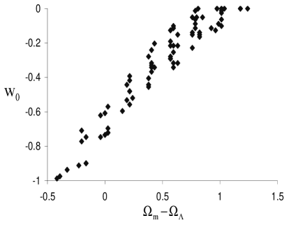
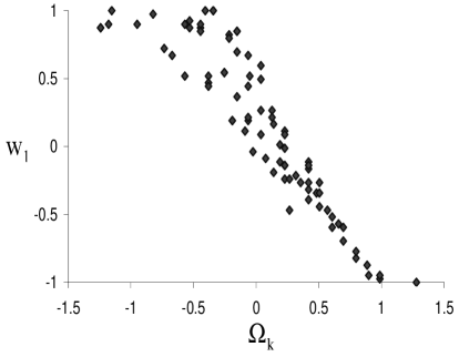
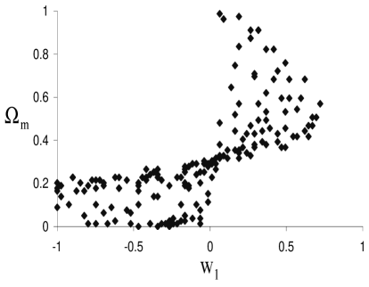
Finally, Figure 8 shows the correlations rising between individual parameters of model A and model C when both models are undistinguished at $2\,\sigma$ level ($\Delta\chi^{2}_{\rm min}<6.17$). Linear regressions through the points yield :

$$w_{0} \sim \displaystyle\frac{2}{3}\,\left(\Omega_{m}-\Omega_{\Lambda}-1\right),$$ (19)

$$w_{1} \sim \Omega_{m}+\Omega_{\Lambda}-1\,\,=-\Omega_{k}.$$ (20)

This demonstrates the degeneracy between the curvature of an FLRW model and the $w_{1}$ parameter of a model C. Note that by construction, model C with $w_{0}=-1$ and $w_{1}=0$ is identical to an FLRW model with $\Omega_{m}=0.3$ and $\Omega_{\Lambda}=0.7$. This result is basically reproduced by the relations (19) and (20).

5.2 Analysis of data generated with model B

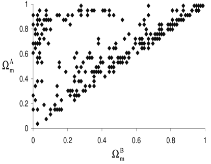
Figure 9 shows the expected degeneracies  if the true model is a model B. The irregurar distribution of the best fit positions in the parameter space of model B denotes its stronger sensitivity to the statistical noise. Moreover, since we looked at the $\chi^{2}_{\rm min}$ scanning parameter space from $\Omega_{m}=0$ to $\Omega_{m}=1$, we find an accumulation of points in the upper left corner of the parameter space of model B, as expected from the form of the degeneracy curves shown in Figure 3. Note that the first row of Figure 9 shows again the degeneracy between $\Omega_{k}$ and $w_{0}$, as already noted in Figure 7 : a flat model B with $w_{0}\not=-1$ can be confused with an FLRW model with spatial curvature.

Figure 10 shows the possible error on the estimate of $\Omega_{m}$ and $w_{0}$, when the correct model B is not used to fit the data. Although there is no significant difference in terms of $\chi^{2}_{\rm min}$, fitting the data with an FLRW model yields values for $\Omega_{m}$ larger than or equal to the exact value (upper plot), and fitting the data with a model C often give rise to value of $w_{0}$ larger than or equal to the correct one (lower plot).

5.3 Analysis of data generated with model C

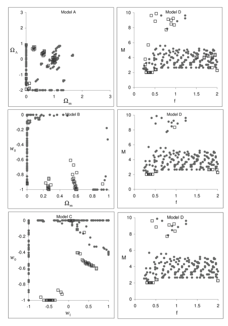
Figure 11 shows the best fit positions in the parameter spaces of models A, B and D when model C has been used as a fiducial model. One can see that :
$-$ First, the $\chi^{2}_{\rm min,A}$ are all located in a region charaterized by $\,\Omega_{m}+\Omega_{\Lambda}<1$ and $\,\Omega_{m}-\Omega_{\Lambda}<1$. This confirms what has been obtained in Figure 7 (cf. second plot of model A on Figure 7).
$-$ Second, as expected, the $\Delta\,\chi^{2}_{\rm min}$ between models B and C less than $6.17$ are usually associated to the model C with $w_{1}\sim 0$, but only if $w_{0}>-0.4$.
$-$ Third, as previously noted, most of the $\chi^{2}_{\rm min}$ positions in the parameter space of model D are located in a region where the scalar field is presently starting to evolve toward the minimum of its potential, i.e. $w_{x}(z)$ leaves the value $-1$ and approaches unity, with $\Omega_{\phi}>\Omega_{m}$. This is why in most cases, the corresponding squares in model C are characterized by $w_{1}\geq 0$.

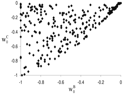
Figure 12 shows the correlation between the best fit values of $w_{1}$ obtained with the true model (C) and the best fit values of $\Omega_{m}$ obtained with a wrong model (B), when $\Delta\chi^{2}_{\rm min}<6.17$. If the true value of $w_{1}$ is positive (negative), then the value of $\Omega_{m}$ found with the wrong model will be larger (smaller) than the true one ($\Omega_{m}=0.3$).

5.4 Analysis of data generated with model D

Finally, Figure 13 presents results obtained using samples generated with model D. It clearly appears that most of the $\chi_{\rm min}^{2}$ positions corresponding to $\Delta\chi^{2}_{\rm min}>6.17$ are located on the edges of the parameter spaces of the wrong models. So if the cosmological model chosen by Mother Nature is a PNGB model, it could be difficult to obtain a good fit with one of the three wrong models A, B or C. Moreover, the presence of some points outside the region of model D used for generating samples denotes a sensitivity to statistical noise. Note that most of the squares in the parameter space of model A of this figure appear like three bundles located at $\Omega_{m}\sim 1-\Omega_{\Lambda}\sim 0.3,0.6$ and $1$. This is due to the strong dependence of $\Omega_{m}$ in model D with $M$ when the scalar field is still frozen and acts like a cosmological constant (cf. horizontal lines for $\Omega_{m}$ in Figure 2). The more precise is the grid used for the data processing in model D, the more those squares will appear uniformly distributed on the line $\Omega_{m}+\Omega_{\Lambda}=1$ in the parameter space of model A.

True model		A			B			C			D
	$\Omega_{m,i}=0.1-(1-i)/5$			$\Omega_{m,i}=0.05+(i-1)/10$			$w_{0,i}=-0.05+(1-i)/10$			$f_{i}=0.4+1.6(i-1)/9$
	$\Omega_{\Lambda,j}=-0.9+0.2(j-1)$			$w_{0,j}=-0.05-(j-1)/10$			$w_{1,j}=-0.95(2j-11)/9$			$M_{j}=2+(j-1)/3$
Compared with	B	C	D	A	C	D	A	B	D	A	B	C
$P(\Delta\chi^{2}_{\rm min}<11.8)$	$19\,\%$	$31\,\%$	$14\,\%$	$98\,\%$	$93\,\%$	$82\,\%$	$95\,\%$	$68\,\%$	$40\,\%$	$35\,\%$	$23\,\%$	$23\,\%$
$P(\Delta\chi^{2}_{\rm min}<6.17)$	$15\,\%$	$27\,\%$	$9\,\%$	$95\,\%$	$93\,\%$	$72\,\%$	$79\,\%$	$59\,\%$	$26\,\%$	$29\,\%$	$20\,\%$	$21\,\%$
$P(\Delta\chi^{2}_{\rm min}<-11.8)$	$0\,\%$	$0\,\%$	$0\,\%$	$0\,\%$	$0\,\%$	$0\,\%$	$0\,\%$	$0\,\%$	$<1\,\%$	$6\,\%$	$7\,\%$	$8\,\%$

Table 4: Probabilities to obtain misleading results when the true model is model A, B, C and D at the $3\,\sigma$ level ($P(\Delta\chi^{2}_{\rm min}<11.8)$) and at the $2\,\sigma$ level ($P(\Delta\chi^{2}_{\rm min}<6.17)$). $P(\Delta\chi^{2}_{\rm min}<-11.8)$ is the probability to exclude the right model at the $3\,\sigma$ level. All these values are associated to the limits on the parameter spaces explored for generating the data.

An important remark has to be made at this point : Figures 9, 11 and 13 show that, whatever the true model is, a FLRW model with $\Omega_{m}=0.3$ and $\Omega_{\Lambda}=0.7$ ($w=-1$) cannot be rejected on the basis of the SNAP observations.

5.5 Probability to select the correct model

Table 4 shows the probabilities to obtain misleading results when the true model is model A, B, C and D at the $3\,\sigma$ level ($P(\Delta\chi^{2}_{\rm min}<11.8)$) and at the $2\,\sigma$ level ($P(\Delta\chi^{2}_{\rm min}<6.17)$). It also presents the probability to exclude the right model at the $3\,\sigma$ level ($P(\Delta\chi^{2}_{\rm min}<-11.8)$). They give an idea of the degree of degeneracy between the models, with respect to the computation of the luminosity distances. For example, it is difficult to identify a true model B among wrong models : the probabilities to confuse model B with model A, C and D are respectively $95\,\%$, $93\,\%$ and $72\,\%$, at $2\,\sigma$ level. Model C cannot be distinguished from models A, B and D in $79\,\%$, $59\,\%$ and $26\,\%$ of the cases respectively ($2\,\sigma$ level). Note that the use of model C as fiducial model assumed an exactly known $\Omega_{m}$. An uncertainty on $\Omega_{m}$ will increase the percentages given above. Finally, if the fiducial model is A or D, we can expect to rule out the proposed wrong models with an a priori probability higher than $65\,\%$ at the 3 $\sigma$ level. However this does not preclude a priori a degeneracy between those models any other possible model.

Samples simulated with model D can lead $\Delta\chi^{2}_{\rm min}$ values less than $-11.8$ ($\sim 7\,\%$), which means that the correct model can be excluded at the $3\,\sigma$ level and confirms the sensitivity of model D to the statistical noise. Table 4 also shows that, whatever the true model is (B, C or D), the probability to reject model A at $3\,\sigma$ is low.

The probabilities presented in Table 4 clearly depend on the regions of the different parameter spaces used for the data simulations. However, in order to obtain meaningful results, we chose the parameter ranges surrounding the physical part of the contours presented in Figure 6.

6 Conclusions

Making use of four quintessence models, of which three are mathematically simple and one is coming directly from particle physics, we have first shown that the various cosmological models may predict apparent magnitudes for objects at given redshifts which differ from each other by less than 0.04 mag till $z=2$. These magnitude differences are thus small compared to the intrinsic spread of the SNeIa maximum luminosity (0.15 mag). This indicates that an unambiguous discrimination between the cosmological models will be difficult to reach, with cosmological tests only based on luminosity distances.

Second, we have fitted these models to the present supernovae data and found equally good fits with the four models. Finally, we have explored the discriminatory power of future SNeIa data to constrain the dark energy properties. We have simulated a large number of SNAP data with each particular model and have re-analysed them with the four cosmological models. We have then compared the positions and the values of the $\chi^{2}_{\rm min}$ obtained using wrong models with those obtained with the fiducial model. This led us to confirm the more skeptical conclusions already made in some previous works on the subject (Barger and Marfatia 2001, Astier 2001, Maor et al. 2001, 2002) : some degeneracies between the curvature, the matter density and the equation-of-state of dark energy will be difficult to break at the $3\,\sigma$ level and even at the $2\,\sigma$ and $1\,\sigma$ level. We also found that different estimates of a basic parameter like $\Omega_{m}$ can be obtained, depending on the model used for the data processing. Moreover, whatever the true model is, the presently admitted FLRW model with $\Omega_{m}=0.3$ and $\Omega_{\Lambda}=0.7$ will not be rejected on the basis of the future SNAP observations alone.

In order to compare results expected from SNAP with the ones which could be obtained by other supernovae surveys, we have also generated data samples from models C and D for another redshift distribution : 2050 SNeIa between $z=0$ and $z=0.5$ and 50 between $z=2$ and $z=2.5$ (with $\sigma_{i}$ = 0.15 mag). This distribution reflects future observations to be made with the 4m Liquid Mirror Telescope (see ILMT URL) and with the Next Generation Space Telescope (see NGST URL). No significant difference has been found with the results presented here.

Many recent papers discussed the strong constraints that could be expected from future SNeIa data on cosmological parameters. However, the most important question is : how can we be sure that we consider the right model ? Indeed how useful are strong constraints on cosmological parameters if they do not describe the model chosen by Mother Nature ? The degeneracy problem presented in this paper is expected to affect every cosmological test using luminosity distance. Therefore it will be very difficult for SNAP alone to obtain any strong and safe constraints on the cosmological parameters. However, we expect that the combination of the CMB data with the future SNAP ones could help to break some of the luminosity distance degeneracies. This fact is already known in the framework of a single cosmological model (see e.g. Huterer & Turner 2001, Frieman et al. 2002, Bean & Melchiorri 2002).

References

- [\citeauthoryearAbbott1998] Abbott L., 1998, Sci. Am. 258, 106
- [\citeauthoryearAstier2001] Astier P., 2001, Phys. Lett. B 500, 8
- [\citeauthoryearBarger & Marfatia2001] Barger V., Marfatia D., 2001, Phys. Lett. B 498, 67
- [\citeauthoryearBean & Melchiorri2002] Bean R., Melchiorri A., 2002, Phys. Rev. D 65, 041302
- [\citeauthoryearCaldwell2002] Caldwell R.R., 2002, Phys. Lett. B 545, 23
- [\citeauthoryearCarroll et al.1992] Carroll S.M., Press W.H., Turner E. L., 1992, ARAA 30, 499
- [\citeauthoryearChiba & Nakamura2000] Chiba T., Nakamura T., 2000, Phys. Rev. D 62, 121301
- [\citeauthoryearChoubey et al.2002] Choubey, S., et al., 2002, preprint hep-ph/0209222
- [\citeauthoryearDi Pietro & Demaret2001] Di Pietro E., Demaret J., 2001, Int. J. Mod. Phys. D 10, 231
- [\citeauthoryearFerreira & Joyce1998] Ferreira P.G., Joyce M., 1998, Phys. Rev. D 58, 023503
- [\citeauthoryearFrieman et al.1992] Frieman J.A., Hill C.T., Watkins R., 1992, Phys. Rev. D 46, 1226
- [\citeauthoryearFrieman et al.1995] Frieman J.A. et al., 1995, Phys. Rev. Lett. 75, 2077
- [\citeauthoryearFrieman & Waga1998] Frieman J.A., Waga I., 1998, Phys. Rev. D 57, 4642
- [\citeauthoryearFrieman et al.2002] Frieman J.A. et al., 2002, preprint astro-ph/0208100
- [\citeauthoryearFukuda et al.1998] Fukuda, Y., et al., 1998, Phys. Rev. Lett. 81, 1562
- [\citeauthoryearGerke & Efstathiou2002] Gerke B.F., Efstathiou G., 2002, M.N.R.A.S. 335, 33
- [\citeauthoryearGoliath et al.2001] Goliath M. et al., 2001, A& A 380, 6
- [\citeauthoryearGonzález-Díaz2000] González-Díaz P.F., 2000, Phys. Rev. D 62, 023513
- [\citeauthoryearHuterer & Turner1999] Huterer D., Turner M.S., 1999, Phys. Rev. D 60, 081301(R)
- [\citeauthoryearHuterer & Turner2001] Huterer D., Turner M.S., 2001, Phys. Rev. D 64, 123527
- [\citeauthoryearILMT2002] ILMT URL : http://vela.astro.ulg.ac.be/themes/telins/lmt/
- [\citeauthoryearMaor et al.2001] Maor I., Brustein R., Steinhardt P.J., 2001, Phys. Rev. Lett.86, 6
- [\citeauthoryearMaor et al.2002] Maor I. et al., 2002, Phys. Rev. D 65, 123003
- [\citeauthoryearMikheyev & Smirnov1985] Mikheyev S.P., Smirnov A., 1985, Sov. J. Nucl. Phys. 42, 913
- [\citeauthoryearNakamura & Chiba1999] Nakamura T., Chiba T., 1999, MNRAS 306, 696
- [\citeauthoryearNg & Wiltshire2001a] Ng S.C.C., Wiltshire D., 2001a, Phys. Rev. D 63, 023505
- [\citeauthoryearNg & Wiltshire2001b] Ng S.C.C., Wiltshire D., 2001b, Phys. Rev. D 64, 123519
- [\citeauthoryearNGST2002] NGST URL : http://ngst.gsfc.nasa.gov/
- [\citeauthoryearParodi et al.2000] Parodi B.R. et al., 2000, ApJ 540, 634
- [\citeauthoryearPeebles & Ratra1988] Peebles P.J.E., Ratra B., 1988, ApJ 325, L17
- [\citeauthoryearPeebles & Ratra2002] Peebles P.J.E., Ratra B., 2002, pre-print astro-ph/0207347
- [\citeauthoryearPerlmutter et al.1999] Perlmutter S. et al., 1999, ApJ 517, 565 [P99]
- [\citeauthoryearRatra & Peebles1988] Ratra B., Peebles P.J.E., 1988, Phys. Rev. D 37, 3406
- [\citeauthoryearRiess et al.1998] Riess A.G. et al., 1998, AJ 116, 1009
- [\citeauthoryearSahni et al.2000] Sahni V., Starobinsky A., 2000, Int. J. Mod. Phys. D 9, 373
- [\citeauthoryearSaini et al.2000] Saini T.D. et al., 2000, Phys. Rev. Lett. 85, 1162
- [\citeauthoryearSNAP2002] SNAP URL : http://snap.lbl.gov/
- [\citeauthoryearSteinhardt et al.1999] Steinhardt P.J., Wang L., Zlatev I., 1999, Phys. Rev. D 59, 123504
- [\citeauthoryearWaga & Frieman2000] Waga I., Frieman J. A., 2000, Phys. Rev. D 62, 043521
- [\citeauthoryearWeinberg1989] Weinberg S., 1989, Rev. Mod. Phys. 61, 1
- [\citeauthoryearWeller & Albrecht2001] Weller J., Albrecht A., 2001, Phys. Rev. Lett. 86, 1939
- [\citeauthoryearWeller & Albrecht2002] Weller J., Albrecht A., 2002, Phys. Rev. D 65, 103512
- [\citeauthoryearWetterich1988] Wetterich C., 1988, Nucl. Phys. B 302, 668
- [\citeauthoryearWolfenstein1979] Wolfenstein L., 1979, Phys. Rev. D 17, 2369