Numerical Simulation of Non-Gaussian Random Fields
with Prescribed Marginal Distributions and Cross-Correlation Structure II: Multivariate Random Fields

Abstract

We provide theoretical procedures and practical recipes to simulate non-Gaussian correlated, homogeneous random fields with prescribed marginal distributions and cross-correlation structure, either in a $N$-dimensional Cartesian space or on the celestial sphere. We illustrate our methods using far-infrared maps obtained with the Infrared Space Observatory. However, the methodology presented here can be used in other astrophysical applications that require modeling correlated features in sky maps, for example, the simulation of multifrequency sky maps where backgrounds, sources and noise are correlated and can be modeled by random fields.

1 Introduction

Random fields are widely used in astrophysics to model realistic scenarios of physical processes that depend on random components. For example, they are widely used in cosmology to model different types of galactic and extragalactic backgrounds (e.g., Martinez & Saar, 2001). The physical characteristics of the backgrounds are translated into statistical characteristics of the field. The fields are usually required to be ergodic so that information about the model can be extracted from a single realization of the field. In addition, they are assumed to be isotropic (the correlation between two points depends only on the distance that separates them) or homogeneous (the correlation depends on the difference of their position vectors) to reflect the geometry of the cosmological model. Given the complexity of the cosmological models, characteristics of the fields are usually studied via Monte Carlo simulations where model predictions are compared with observations.

To simulate a Gaussian random field we only need to specify the mean and spectrum (or correlation function) but there are non-Gaussian models whose predictions also have to be tested against observations. For example, standard inflationary models predict Gaussian temperature fluctuations of the cosmic microwave background but there are other cosmological models that predict non-Gaussian fluctuations (Avelino et al., 1998; Peebles, 1999). Homogeneous non-Gaussian random fields are more difficult to define and simulate, and since they are not uniquely determined by their first two moments, we often have to accept only a partial second order description of the fields.

Vio, Andreani & Wamsteker (2001) (hereafter VAW) presented numerical methods for the simulation of homogeneous scalar random fields $R(\boldsymbol{t})$ with prescribed one-dimensional distribution function (marginal distribution) $F_{R}(r)$ and correlation structure. These methods can be used, for example, to generate cosmic microwave background maps with a given spectrum and a marginal distribution that allows for asymmetry or kurtosis in the pixel temperatures. In this paper we generalize these methods to the case of pair-wise correlated random fields defined on the same physical space. This will allow us, for example, to simulate backgrounds and source fields that are not independent, as in star-forming regions where the already formed stars are linked to the surrounding gaseous and dusty environment from which they originate.

We consider random fields defined in $N$-dimensional “parameter spaces” where the coordinates $\boldsymbol{t}=(t_{1},t_{2},\ldots,t_{N})$ may correspond to spatial/angular coordinates (spatial random fields), time (time processes), a mix of these two (spatio-temporal random fields), or to even more general situations. We also consider the case of random fields defined on the sphere, that is, random fields that depend only on the direction in the sky. If the multivariate random field is $\boldsymbol{R}(\boldsymbol{t})=\{R_{1}(\boldsymbol{t})$, $R_{2}(\boldsymbol{t})$,$\ldots$, $R_{M}(\boldsymbol{t})\}$, the goal is to generate a field with components $R_{i}$ having (possibly different) prescribed marginal distributions $F_{R_{i}}(r_{i})$, prescribed correlation functions, and prescribed pair-wise cross-correlations.

In theory, a complete description of a random field requires the definition of all finite-dimensional joint distributions, but, unless the field is Gaussian, this is a terribly difficult task. In practical applications one only considers a second order description of the field that specifies the marginals $F_{R_{i}}(r_{i})$, the means $\mu_{R_{i}}={\rm E}[\,R_{i}(\boldsymbol{t})\,]$ and the cross-covariance functions

$$\xi_{R_{i}R_{j}}(\boldsymbol{t}_{1},\boldsymbol{t}_{2})={\rm E}\left[\,(R_{i}(\boldsymbol{t}_{1})-\mu_{R_{i}})~{}(R_{j}(\boldsymbol{t}_{2})-\mu_{R_{j}})\,\right],$$ (1)

where ${\rm E}[\cdot]$ stands for expected value (ensemble average).

As mentioned before, it is often possible, even necessary, to adopt some simplifying assumptions like isotropy or homogeneity of the field $\boldsymbol{R}(\boldsymbol{t})$. In the multidimensional context, isotropy means that the cross-covariance function depends on the length $\tau=\|\boldsymbol{\tau}\|$ of the vector $\boldsymbol{\tau}=\boldsymbol{t}_{1}-\boldsymbol{t}_{2}$ but not on its direction: $\xi_{R_{i}R_{j}}(\boldsymbol{t}_{1},\boldsymbol{t}_{2})=\xi_{R_{i}R_{j}}(\|\boldsymbol{t}_{1}-\boldsymbol{t}_{2}\|)$. In this case the cross-correlation function (normalized covariance function) depends only on $\tau$

$$\boldsymbol{\rho}_{\boldsymbol{R}}(\tau)=\left(\begin{array}[]{ccc}\rho_{R_{1}R_{1}}(\tau)&&\rho_{R_{1}R_{M}}(\tau)\\ \vdots&\ddots&\vdots\\ \rho_{R_{M}R_{1}}(\tau)&&\rho_{R_{M}R_{M}}(\tau)\end{array}\right),$$ (2)

where

$$\rho_{R_{i}R_{j}}(\tau)={\rm E}\left[\frac{(R_{i}(\boldsymbol{t})-\mu_{R_{i}})~{}(R_{j}(\boldsymbol{t}+\boldsymbol{\tau})-\mu_{R_{j}})}{\sigma_{R_{i}}\sigma_{R_{j}}}\right]$$ (3)

and $\sigma_{R_{i}}^{2}$ is the variance corresponding to the marginal $F_{R_{i}}(r_{i})$. By definition, $\rho_{R_{i}R_{i}}(0)=1$ for $i=1,2,\ldots,M$.

Although the isotropic case is of great interest in astronomical applications, here we consider multidimensional homogeneous random fields in general, that is, random fields whose covariance function depends on $\boldsymbol{\tau}$. In this case, the correlation function $\boldsymbol{\rho}_{\boldsymbol{R}}(\boldsymbol{\tau})$ is defined as in equation (2) but with $\boldsymbol{\tau}$ instead of $\tau$.

The rest of the paper is organized as follows. In Section 2 we describe a general procedure for generating non-Gaussian random fields by point-wise transformations of Gaussian ones. In Section 3 we provide practical recipes for the methods outlined in Section 2 and show how they can be used in either $N$-dimensional Cartesian spaces or on the celestial sphere. Section 4 presents some examples. We show simulated maps of the background and localized source field components of a far-IR sky map of the Infrared Space Observatory (ISO). In the ISO map, the locations and intensities of the sources are correlated with the background field and only a multidimensional simulation may reproduce such physical characteristic.

2 Transforming Gaussian fields to non-Gaussian

In Section 3.2 we discuss methods for generating homogeneous Gaussian random fields with a prescribed correlation structure. The procedures are straightforward, at least in principle, while, in contrast, generating homogeneous non-Gaussian fields is not a trivial task. Fortunately, a large family of such fields can be obtained via pointwise transformations of homogeneous Gaussian fields. These transformations are the basis of the methods used in VAW to simulate non-Gaussian scalar random fields. In this paper we generalize them to the multivariate case.

We propose the following procedure for simulating multidimensional homogeneous non-Gaussian fields $\boldsymbol{R}(\boldsymbol{t})$ with prescribed cross-correlation structure $\boldsymbol{\rho}_{\boldsymbol{R}}(\boldsymbol{\tau})$ and one-dimensional marginals $F_{R_{i}}(r)$: (a) Generate a zero-mean, unit-variance, homogeneous multivariate Gaussian field $\boldsymbol{X}(\boldsymbol{t})$ with a fixed cross-correlation structure $\boldsymbol{\rho}_{\boldsymbol{X}}(\boldsymbol{\tau})$; (b) transform $\boldsymbol{X}(\boldsymbol{t})$ to a non-Gaussian field $\boldsymbol{R}(\boldsymbol{t})$ via

$$\boldsymbol{R}(\boldsymbol{t})=\boldsymbol{g}[\,\boldsymbol{X}(\boldsymbol{t})\,],$$ (4)

where $\boldsymbol{g}(\cdot)=\{g_{1}(\cdot),g_{2}(\cdot),\ldots,g_{M}(\cdot)\}$. The problem is to determine a Gaussian field $\boldsymbol{X}(\boldsymbol{t})$ and functions $\{g_{i}\}$ that transform $\boldsymbol{\rho}_{\boldsymbol{X}}(\boldsymbol{\tau})$ into $\boldsymbol{\rho}_{\boldsymbol{R}}(\boldsymbol{\tau})$.

As discussed in VAW, given marginals $\{F_{R_{i}}(r)\}$ with no atoms (a concentration of a finite probability mass at a point), the integral transform

$$R_{i}(\boldsymbol{t})=g_{i}[\,X_{i}(\boldsymbol{t})\,]=F^{-1}_{R_{i}}\{\,F_{X}[\,X_{i}(\boldsymbol{t})\,]\,\};\qquad i=1,2,\ldots,M,$$ (5)

where $F_{X}$ denotes the standard Gaussian distribution function and $F^{-1}_{R_{i}}$ is the inverse distribution function of $R_{i}(\boldsymbol{t})$, provides a random field with marginals $\{F_{R_{i}}(r)\}$. Since $g_{i}(\cdot)=F^{-1}_{R_{i}}\{F_{X}(\cdot)\}$ is a strictly monotonic function, transformation (5) is invertible and $\rho_{R_{i}R_{j}}(\boldsymbol{\tau})$ can be calculated through

$$\rho_{R_{i}R_{j}}(\boldsymbol{\tau})=\frac{1}{\sigma_{R_{i}}\sigma_{R_{j}}}\int_{-\infty}^{\infty}\int_{-\infty}^{\infty}[g_{i}(x_{1})-\mu_{R_{i}}]~{}[g_{j}(x_{2})-\mu_{R_{j}}]~{}\phi(x_{1},x_{2};\rho_{X_{i}X_{j}}(\boldsymbol{\tau}))~{}dx_{1}~{}dx_{2},$$ (6)

where, $x_{1}=x(\boldsymbol{t})$, $x_{2}=x(\boldsymbol{t}+\boldsymbol{\tau})$, and

$$\phi(x_{1},x_{2};\,\rho_{X_{i}X_{j}}(\boldsymbol{\tau})\,)=\frac{1}{2\pi\,[\,1-\rho_{X_{i}X_{j}}^{2}(\boldsymbol{\tau})\,]^{1/2}}~{}\exp\left(-\frac{x_{1}^{2}+x_{2}^{2}-2\rho_{X_{i}X_{j}}(\boldsymbol{\tau})\,x_{1}x_{2}}{2\,[\,1-\rho_{X_{i}X_{j}}^{2}(\boldsymbol{\tau})\,]}\right).$$ (7)

For example, Figure 1 shows the relationship between $\rho_{X_{i}X_{j}}$ and $\rho_{R_{i}R_{j}}$ for some standard marginal distributions.

Equation (6) can be used to solve for the cross-correlations of a Gaussian field that transform to those of the non-Gaussian field. Ogorodnikov & Prigarin (1996) show that $\rho_{R_{i}R_{j}}(\boldsymbol{\tau})$ is a monotonic increasing function of $\rho_{X_{i}X_{j}}(\boldsymbol{\tau})$ and that (6) does not present invertibility problems. However, although via this inversion it is always possible to map a value of $\rho_{X_{i}X_{j}}(\boldsymbol{\tau})$ to its corresponding value $\rho_{R_{i}R_{j}}(\boldsymbol{\tau})$, there is no guarantee that the resulting $\rho_{X_{i}X_{j}}(\boldsymbol{\tau})$ is in fact a non-negative definite function and hence a valid cross-correlation function. This condition must be checked (see below). There are also restrictions on the distributions $F_{R_{i}}$ that can be obtained. For example, as already shown in VAW, the values of $\rho_{R_{i}R_{j}}$ that can be inverted are those in the interval $\rho_{R_{i}R_{j}}\in[\,\rho^{*}_{1},\rho^{*}_{2}\,]$, where $\rho^{*}_{1}$ and $\rho^{*}_{2}$ correspond, respectively, to the values of $-1$ and $1$ of $\rho_{X_{i}X_{j}}$ for a fixed function $\boldsymbol{g}$. This is clearly seen in Figure 1 where relationships between $\rho_{R_{i}R_{j}}$ and $\rho_{X_{i}X_{j}}$ for some classic distribution functions are shown.

To conclude this section we note that the fields $R_{i}(\boldsymbol{t})$ can be forced to have a chosen mean $\tilde{\mu}_{i}$ and variance $\tilde{\sigma}^{2}_{i}$ by applying the transformation

$$\tilde{R}_{i}(\boldsymbol{t})=\tilde{\mu}_{R_{i}}+\frac{R_{i}(\boldsymbol{t})-\mu_{R_{i}}}{\sigma_{R_{i}}}~{}~{}\tilde{\sigma}_{R_{i}}.$$ (8)

without modifying the cross-correlation structure.

3 Practical recipes

To simulate a non-Gaussian field $\boldsymbol{R}(\boldsymbol{t})$ via equations (5) and (6) we need to (a) determine the appropriate cross-correlation functions $\rho_{X_{i}X_{j}}(\boldsymbol{\tau})$ of the Gaussian fields $X_{i}(\boldsymbol{t})$ to be transformed, (b) check that $\boldsymbol{\rho}_{\boldsymbol{X}}(\boldsymbol{\tau})$ is a non-negative definite function, and (c) simulate the Gaussian fields $X_{i}(\boldsymbol{t})$.

3.1 Solving the inverse problem

In principle, $\rho_{X_{i}X_{j}}(\boldsymbol{\tau})$ can be obtained by inverting equation (6) but this procedure is computationally expensive. Instead, since the relationship between $\rho_{X_{i}X_{j}}(\boldsymbol{\tau})$ and $\rho_{R_{i}R_{j}}(\boldsymbol{\tau})$ is generally smooth, it is sufficient to choose a set of values in the interval $[-1,~{}1]$ for $\rho_{X_{i}X_{j}}(\boldsymbol{\tau})$ and to solve for their corresponding values $\rho_{R_{i}R_{j}}(\boldsymbol{\tau})$ via the numerical integration of equation (6). The complete relationship between the two correlation functions may be obtained by spline interpolation. The interpolated function is then used to determine $\rho_{X_{i}X_{j}}(\boldsymbol{\tau})$ as a function of $\boldsymbol{\tau}$.

The function $\boldsymbol{\rho}_{\boldsymbol{X}}(\boldsymbol{\tau})$ has to be non-negative definite to correspond to a homogeneous field. This means that every $\rho_{X_{i}X_{j}}(\boldsymbol{\tau})$ is a non-negative definite function and that the matrix $\boldsymbol{\rho}_{\boldsymbol{X}}(\boldsymbol{\tau})$ is non-negative definite for each $\boldsymbol{\tau}$. To check this conditions just note that the Fourier transform of $\rho_{X_{i}X_{j}}(\boldsymbol{\tau})$, which provides the cross-spectrum between the fields $X_{i}(\boldsymbol{t})$ and $X_{j}(\boldsymbol{t})$, must be a non-negative function. It is therefore sufficient to check that the $N$-fold Fourier transform of $\rho_{X_{i}X_{j}}(\boldsymbol{\tau})$ does not take negative values for any pair $i,j$. In addition, for any fixed $\boldsymbol{\tau}$, $\boldsymbol{\rho}_{\boldsymbol{X}}(\boldsymbol{\tau})$ has to be a non-negative definite matrix and therefore its eigenvalues have to be non-negative. This is automatically checked within the field simulation procedure described in the sections below.

3.2 Simulating Gaussian multivariate random fields in $R^{N}$

To simulate a zero-mean homogeneous multivariate Gaussian field $\boldsymbol{X}(\boldsymbol{t})$ of unit-variance components $X_{i}(\boldsymbol{t})$ and prescribed cross-correlation functions, we use the spectral representation that decomposes the field as a superposition of uncorrelated sinusoids of different frequencies and random amplitudes

$$X_{i}(\boldsymbol{t})=\underbrace{\int_{-\infty}^{+\infty}\int_{-\infty}^{+\infty}\dots\int_{-\infty}^{+\infty}}_{N-fold}{\rm e}^{\iota 2\pi\boldsymbol{k}\cdot\boldsymbol{t}}~{}dZ_{i}(\boldsymbol{k}),\qquad i=1,2,\ldots,M;$$ (9)

where $\iota=\sqrt{-1}$, $\boldsymbol{k}\cdot\boldsymbol{t}$ is the inner product between the wave number and position vectors, and $dZ_{i}(\boldsymbol{k})$ are random orthogonal increments satisfying (Priestley, 1981)

$$E[\,dZ_{i}(\boldsymbol{k})\,] = 0,$$

$$E[\,dZ_{i}(\boldsymbol{k})~{}dZ^{*}_{j}(\boldsymbol{k}^{\prime})\,] = 0,~{}~{}~{}~{}\boldsymbol{k}\neq\boldsymbol{k}^{\prime},~{}~{}i,j=1,\ldots,M,$$ (10)

$$E[\,dZ_{i}(\boldsymbol{k})~{}dZ^{*}_{j}(\boldsymbol{k})\,] = S_{ij}(\boldsymbol{k})~{}\boldsymbol{d}\boldsymbol{k},$$

where “$~{}{}^{*}~{}$” indicates the complex conjugate operator, $\boldsymbol{d}\boldsymbol{k}=dk_{1}\cdot dk_{2}\cdot\ldots\cdot dk_{N}$, and $S_{ij}(\boldsymbol{k})$ is the cross-spectrum of the fields $X_{i}(\boldsymbol{t})$ and $X_{j}(\boldsymbol{t})$. If the field is Gaussian, then $dZ_{i}(\boldsymbol{k})$ is an $M$-dimensional zero-mean complex Gaussian random variable with correlation matrix determined by the cross-spectrum

$$\boldsymbol{S}_{\boldsymbol{X}}(\boldsymbol{k})=\left(\begin{array}[]{ccc}S_{11}(\boldsymbol{k})&&S_{1M}(\boldsymbol{k})\\ \vdots&\ddots&\vdots\\ S_{M1}(\boldsymbol{k})&&S_{MM}(\boldsymbol{k})\end{array}\right),$$ (11)

for any fixed $\boldsymbol{k}$. Increments corresponding to different $\boldsymbol{k}$’s are independent.

A similar spectral representations for homogeneous random fields defined on a discrete parameter space is (e.g., Ruan & McLaughlin, 1998)

$$X_{i}(\boldsymbol{t})=\underbrace{\sum\sum\dots\sum}_{N-fold}{\rm e}^{\iota 2\pi\boldsymbol{k}\cdot\boldsymbol{t}}\Delta Z_{i}(\boldsymbol{k});\qquad i=1,2,\ldots,M,$$ (12)

(the sums are understood to be over all the discrete wave numbers) where

$$E[\,\Delta Z_{i}(\boldsymbol{k})\,] = 0,$$

$$E[\,\Delta Z_{i}(\boldsymbol{k})~{}\Delta Z^{*}_{j}(\boldsymbol{k}^{\prime})\,] = 0,~{}~{}~{}~{}\boldsymbol{k}\neq\boldsymbol{k}^{\prime},~{}~{}i,j=1,\ldots,M,$$ (13)

$$E[\,\Delta Z_{i}(\boldsymbol{k})~{}\Delta Z^{*}_{j}(\boldsymbol{k})\,] = S_{ij}(\boldsymbol{k})~{}\boldsymbol{\Delta}\boldsymbol{k},$$

$\boldsymbol{\Delta}\boldsymbol{k}=\Delta k_{1}\cdot\Delta k_{2}\cdot\ldots\cdot\Delta k_{N}$. The discrete representation (12) approaches the continuous one (9) as $|\boldsymbol{\Delta}\boldsymbol{k}|$ approaches zero. As in the one-dimensional case, the cross-spectrum $\boldsymbol{S}_{\boldsymbol{X}}(\boldsymbol{k})$ is related to $\boldsymbol{\rho}_{\boldsymbol{X}}(\boldsymbol{\tau})$ through the ($N$-fold) discrete Fourier transform. Therefore, under regularity conditions on $\boldsymbol{\rho}_{\boldsymbol{X}}(\boldsymbol{\tau})$, $\boldsymbol{S}_{\boldsymbol{X}}(\boldsymbol{k})$ is Hermitian and non-negative definite for each value of $\boldsymbol{k}$, and can be factored as

$$\boldsymbol{S}_{\boldsymbol{X}}(\boldsymbol{k})=\boldsymbol{H}(\boldsymbol{k})\boldsymbol{H}^{*}(\boldsymbol{k})=\sum_{l=1}^{M}H_{il}(\boldsymbol{k})H^{*}_{jl}(\boldsymbol{k}).$$ (14)

We can also rewrite $\Delta Z_{i}(\boldsymbol{k})$ in the form

$$\Delta Z_{i}(\boldsymbol{k})=\sum_{l=1}^{M}H_{il}(\boldsymbol{k})~{}\xi(\boldsymbol{k})~{}{\rm e}^{\iota\theta_{l}(\boldsymbol{k})}|\boldsymbol{\Delta}\boldsymbol{k}|^{1/2},$$ (15)

where $\xi(\boldsymbol{k})$ are independent Rayleigh random deviates and $\theta_{l}(\boldsymbol{k})$ are independent phase angles uniformly distributed on the interval $[0,2\pi]$. We obtain a random phase representation of the field by inserting this equation into expression (12)

$$X_{i}(\boldsymbol{t})=\underbrace{\sum\sum\dots\sum}_{N-fold}\sum_{l=1}^{M}{\rm e}^{\iota 2\pi\boldsymbol{k}\cdot\boldsymbol{t}}H_{il}(\boldsymbol{k})~{}\xi(\boldsymbol{k})~{}{\rm e}^{\iota\theta_{l}(\boldsymbol{k})}|\boldsymbol{\Delta}\boldsymbol{k}|^{1/2}.$$ (16)

Equation (16) can be rewritten in the more revealing form

$$X_{i}(\boldsymbol{t})={\rm IDFT}_{N}\left[\,\sum_{l=1}^{M}H_{il}(\boldsymbol{k})~{}\xi(\boldsymbol{k})~{}{\rm e}^{\iota\theta_{l}(\boldsymbol{k})}\,\right]\cdot|\boldsymbol{\Delta}\boldsymbol{k}|^{1/2},$$ (17)

where “${\rm IDFT}_{N}[\cdot]$” stands for $N$-fold inverse discrete Fourier transform. This leads to the following procedure for the numerical generation of a discrete field $\boldsymbol{X}(\boldsymbol{t})$ characterized by a prescribed $\boldsymbol{\rho}_{\boldsymbol{X}}(\boldsymbol{\tau})$:

1. Determine the cross-spectra $\boldsymbol{S}_{\boldsymbol{X}}(\boldsymbol{k})$ by applying the $N$-fold discrete Fourier transform to $\boldsymbol{\rho}_{\boldsymbol{X}}(\boldsymbol{\tau})$.

2. Factor $\boldsymbol{S}_{\boldsymbol{X}}(\boldsymbol{k})$ as indicated in equation (14).

3. Generate a set of $M$ random Fourier increments from equation (15) using a set of $M$ independent random phase angles uniformly distributed over $[0,2\pi]$, and a set of $M$ independent Rayleigh deviates. The phase angles and the Rayleigh deviates at different wave numbers must be independent. Rayleigh deviates $\xi(\boldsymbol{k})$ can be generated by the transformation $\xi(\boldsymbol{k})=\left[-2~{}\ln u(\boldsymbol{k})\right]^{1/2}$, where $u(\boldsymbol{k})$ is a uniform random number on the interval $[0,1]$ (Ogorodnikov & Prigarin, 1996).

4. Apply the ($N$-fold) inverse Fourier transform of the random Fourier increments to obtain a set of $M$ complex (or $2M$ real) random fields.

Note that the factorization (14) of $\boldsymbol{S}_{\boldsymbol{X}}(\boldsymbol{k})$ is not unique, there are a variety of methods that can be used, some being more stable than others. One possibility is to obtain $\boldsymbol{H}(\boldsymbol{k})$ via the singular value decomposition square root of $\boldsymbol{S}_{\boldsymbol{X}}(\boldsymbol{k})$

$$\boldsymbol{H}(k)=\boldsymbol{S}_{\boldsymbol{X}}^{1/2}(k)=\boldsymbol{M}\boldsymbol{J}^{1/2}\boldsymbol{M}^{-1},$$ (18)

where $\boldsymbol{M}$ is a matrix whose columns are eigenvectors of $\boldsymbol{S}_{\boldsymbol{X}}(k)$, and $\boldsymbol{J}$ is a diagonal matrix containing the corresponding eigenvalues. Alternativeley, one can use the Cholesky factorization, which may be more numerically stable (Popescu, Deodatis & Prevost, 1998). With either factorization it is easy to test if the matrix $\boldsymbol{S}_{\boldsymbol{X}}(\boldsymbol{k})$ is non-negative definite for each $\boldsymbol{k}$. Indeed, if $\boldsymbol{S}_{\boldsymbol{X}}(\boldsymbol{k})$ does not satisfy this condition the algorithm providing the Cholesky factorization does not converge, and the matrix $\boldsymbol{J}$ contains one or more negative entries.

Another point to consider is that, although we are interested in the numerical simulation of real valued random fields, the suggested procedure does not impose the necessary symmetry restrictions on the Rayleigh deviates and phase angles in (16) to avoid complex values of the fields $X_{i}(\boldsymbol{t})$. However, if the Rayleigh deviates and phase angles are generated with no symmetry restrictions, then the resulting field $\{X_{i}(\boldsymbol{t})\}$ is complex with independent real and imaginary parts, each with cross-correlation matrix given by $\boldsymbol{\rho}_{\boldsymbol{X}}(\boldsymbol{\tau})/2$ (e.g., Ruan & McLaughlin, 1998). Thus, the real and the imaginary parts of $\sqrt{2}\,X_{i}(\boldsymbol{t})$ provide two independent real valued realizations of the desired random fields.

3.3 Simulating Gaussian multivariate random fields on a sphere

A zero mean random field $R(\boldsymbol{r})$ on the unit sphere is homogeneous if the covariance of the field between two different directions, $\boldsymbol{r}_{1}$ and $\boldsymbol{r}_{2}$, depends only on the angular distance that separates them. In this case the correlation function can be written as

$$\rho_{RR}(\theta)=\frac{{\rm E}\left[\,R(\boldsymbol{r}_{1})\,R(\boldsymbol{r}_{2})\,\right]}{\sigma^{2}_{RR}},$$ (19)

where $\cos\theta=\boldsymbol{r}_{1}\cdot\boldsymbol{r}_{2}$, and $\sigma^{2}_{RR}={\rm E}\,[\,R(\boldsymbol{r}_{1})^{2}\,]={\rm E}\,[\,R(\boldsymbol{r}_{2})^{2}\,]$. The field has the spectral representation

$$R(\boldsymbol{r})=\sum_{\ell=0}^{\infty}\sum_{m=-\ell}^{\ell}a_{\ell,m}\,Y_{\ell,m}(\boldsymbol{r}),$$ (20)

where $\{Y_{\ell,m}\}$ is a basis of spherical harmonics. The coefficients $\{\,a_{\ell,m}\,\}$ are zero mean complex uncorrelated random variables with variance that depends only on $\ell$

$${\rm E}\left[\,a_{\ell,m}\,a^{*}_{\ell,m}\,\right]=\sigma_{\ell}^{2},$$ (21)

and $\sum_{\ell}\sigma_{\ell}^{2}<\infty$. Similarly, a zero mean multivariate random field $\boldsymbol{R}(\boldsymbol{r})=\{R_{1}(\boldsymbol{r}),...,R_{M}(\boldsymbol{r})\}$ is homogeneous if each $R_{i}$ is a homogeneous field and the pair-wise cross-correlations depend only on the angular distance. In this case the cross-correlation function is as in (2) but with $\theta$ taking the place of $\tau$.

The spectral representation of the cross-correlation function of $\boldsymbol{R}$ is (Yaglom, 1986)

$$\boldsymbol{\rho}_{\boldsymbol{R}}(\theta)=\sum_{\ell}\frac{2\ell+1}{4\pi}\,\boldsymbol{S}_{\ell}\,P_{\ell}(\cos\theta),$$ (22)

where $P_{\ell}$ is the Legendre polynomial of degree $\ell$ and $\{\,\boldsymbol{S}_{\ell}\,\}$ are non-negative definite matrices. The corresponding spectral representation of the multivariate field is

$$\boldsymbol{R}(\boldsymbol{r})=\sum_{\ell,m}\boldsymbol{A}_{\ell,m}\,Y_{\ell,m}(\boldsymbol{r}),$$ (23)

where $\boldsymbol{A}_{\ell,m}$ are $M\times 1$ zero mean complex random vectors with

$${\rm E}\left[\,\boldsymbol{A}_{\ell,m}\,\boldsymbol{A}_{\ell,m}^{*}\,\right] = \boldsymbol{S}_{\ell},$$ (24)

$${\rm E}\left[\,\boldsymbol{A}_{\ell,m}\,\boldsymbol{A}_{\ell,m}^{*}\,\right] = {\bf 0}\quad\quad\mbox{for $\ell\neq\ell^{\prime}$ or $m\neq m^{\prime}$}.$$ (25)

Each matrix $\boldsymbol{S}_{\ell}$ can be factored as in equation (14): $\boldsymbol{S}_{\ell}=\boldsymbol{H}_{\ell}\boldsymbol{H}_{\ell}^{*}.$ As mentioned in the previous section, different factorizations lead to spectral estimates with different variance characteristics. Any such factorization leads to representations like (16) and (17) for Gaussian fields in terms of independent uniform random phases $\theta_{s}(\ell,m)$ and independent Rayleigh deviates $\xi_{s}(\ell,m)$

$$R_{i}(\boldsymbol{r}) = \sum_{\ell,m}\,\Big{[}\,\sum_{s}(\boldsymbol{H}_{\ell})_{ks}\,\xi_{s}(\ell,m)\,e^{\iota\theta_{s}(\ell,m)}\,\Big{]}\,Y_{\ell,m}(\boldsymbol{r})$$ (26)

$$= \mbox{SFT}\Big{[}\,\sum_{s}(\boldsymbol{H}_{\ell})_{ks}\,\xi_{s}(\ell,m)\,e^{\iota\theta_{s}(\ell,m)}\,\Big{]};\qquad i=1,...,M,$$ (27)

where SFT stands for spherical Fourier transform. For discrete implementations of the spherical Fourier transform see, for example, Dilts (1985) and Driscoll & Healy (1994).

4 Examples

We start with a simple numerical simulation. Figure 2 shows a simulation of three two-dimensional, isotropic, random fields with a standard Gaussian $N(0,1)$, a $\chi^{2}_{1}$, and a uniform $U(0,1)$ as marginals, respectively. To illustrate different degrees of correlation in the simulation, we use the cross-correlation matrix

$$\boldsymbol{\rho}_{\boldsymbol{R}}(\tau)=\rho^{0}(\tau)\cdot\left(\begin{array}[]{ccc}1&0.3&0.9\\ 0.3&1&0.4\\ 0.9&0.4&1\end{array}\right).$$ (28)

The procedure used is the one described in Section 3 with a matrix $\boldsymbol{H}(\boldsymbol{k})$ obtained by a Cholesky factorization of $\boldsymbol{S}_{\boldsymbol{X}}(\boldsymbol{k})$. The marginal distributions in the three maps are very different; the Gaussian is symmetric about zero, the $\chi^{2}$ is nonnegative and right skewed, the uniform is bounded between zero and one. However, they all have the same autocorrelation function and there is a clear correlation between every pair of maps; the correlation is stronger between the Gaussian and the uniform because of the 0.9 coefficient in $\boldsymbol{\rho}_{\boldsymbol{R}}$.

4.1 Simulating the components of ISO far-IR maps

VAW presented simulations of ISO far-IR maps but their method was unable to integrate the correlation between the field of localized point sources and the diffuse background. This integration is needed since in the observed data the location and the intensity of the brightest sources are correlated with the brightest regions in the background. As a result, the methodology presented in WAV is unable to satisfactorily reproduce the localized source features of the original ISO map on large scale.

We now show that the methods presented in the previous sections can account for this type of correlation information and efficiently exploit it in generating the simulated map. Figure 3 shows simulations of the random background and source components of a far-IR map obtained by the following procedure. Figure 3a is the observed map, recorded by the ISOPHOT camera (Lemke, Klaas & Abolins, 1996) on board the ISO satellite (Kessler et al., 1996) at $175$ $\mu$m, with a projected size of roughly $40^{\prime}\times 40^{\prime}$ (Dole, et al., 2001). This map is used to generate a Gaussian background field (Figure 3b) via Fourier phase randomization. If physical models of the diffuse background were available, they could also be used to simulate this field.

It is well known that extreme values of distributions can be used to generate point processes. For example, consider $X_{1},...,X_{n}$ uncorrelated Gaussian random variables. Define $N$ as the number of $X_{i}$ above a threshold $\tau$ and $p=P[X_{i}>\tau]$. Then $N$ is a Binomial $B(n,p)$ that can be approximated by a Poisson with $\lambda=np$ for $n$ large and $p$ small. In our case we need more than a point process for the location of the sources, we also need a distribution for their intensity. For this reason we have adopted a different approach based on Gaussian mixtures. These distributions have been successfully used to model outliers and other types of nonstationary behavior in time series (McLachlan & Peel, 2000; Le, Martin & Raftery, 1996). Recall that the distribution of a $k$-component Gaussian mixture is of the form $F(x)=\sum_{i=1}^{k}\alpha_{i}G_{i}(x)$, where the $\alpha_{i}\geq 0$ ($\sum_{i}\alpha_{i}=1$) define the probabilities of sampling from each of the Gaussian distributions $G_{i}$ (note that a Gaussian mixture with more than one component is not Gaussian).

For the ISO example we have used a mixture of two Gaussian components for the marginal distribution of the pixels. The idea is the following. The location of the extreme values of this mixture define the point process, the intensities are defined by the Gaussian distribution of the first mixture component. The second component generates an essentially zero background. For example, Figure 4 shows a realization of the Gaussian mixture used for Figure 3c (the intensities in the original ISO map were normalized to unit standard deviation). We also define a cross-correlation function to correlate the location and intensities of the sources with the Gaussian background in Figure 3b.

Since we do not have a separate image of the source field, in order to fix the parameters of the mixture, we identified point sources by choosing peaks in the original ISO image. The mean and standard deviation of the selected sources were used to define the Gaussian component with a fraction $\alpha$ equal to the proportion of pixels identified as sources. We used a Gaussian centered at zero with a small standard deviation for the second mixture component (see Figure 4). This means that a proportion $1-\alpha$ of the simulated observations are essentially zero. The rest of the observations have an intensity spread about the mean of the observed sources. In practice the Gaussians are truncated to avoid numerical instabilities in the integral transform (5).

Finally we have to choose a cross-correlation matrix. To illustrate the correlation of the sources with the bright regions in the background, we used the cross-correlation function

$$\boldsymbol{\rho}(\tau)=\left(\begin{array}[]{ccc}\rho_{0}(\tau)&\beta\,\rho_{0}(\tau)\\ \beta\,\rho_{0}(\tau)&B(\tau)\\ \end{array}\right),$$ (29)

where $\rho_{0}$ is the auto-correlation function of the original ISO map, $\beta\in[-1,1]$ is a constant, and $B(\tau)$ is the correlation function introduced by the instrument’s smoothing. The choice of this form for $\boldsymbol{\rho}(\tau)$ is based on a lack of sufficient information about the source field. In particular, the cross-correlation of the background and source fields is assumed to be a multiple of $\rho_{0}$ only for illustrative purposes; there are of course applications where this is not true, see for example Mo & White (1996). For the same reason, we decided to assume that the correlations in the source field were introduced only by the Gaussian beam smoothing of the instrument. Figures 3c,d show fields of sparse localized sources for $\beta=0.20$ and $\beta=0.90$, respectively. In both cases, the check described in Section 3.1 has confirmed that $\boldsymbol{\rho}(\tau)$ is a valid cross-correlation matrix for each $\tau$. It is clear that the correlation of the locations and intensities of the sources with the background map of Figure 3b increases with $\beta$.

The application of this methodology for the realistic simulation of far-IR maps recorded by the array cameras on board the Herschel satellite (Pilbratt, 2001) is under investigation. The combination of both physical models and observations is compelling in determining the types of distributions and cross-correlation functions that are appropriate for the particular application under investigation.

5 Summary

We have described spectral methods for the simulation of homogeneous non-Gaussian multivariate random fields with prescribed cross-correlation and marginal distributions. The basic idea is to apply pointwise transformations to homogeneous Gaussian fields to guarantee the homogeneity of the field. The transformations are chosen to obtain the desired marginal distributions and cross-correlation function. The proposed methodology works for a wide range of cross-correlation functions and marginal distributions of general interest. Among these, some Gaussian mixture models may be useful to model fields of localized sources.

We have illustrated the methods by simulating sky maps with background and source components that are physically linked. The same methods can also be applied to simulate and/or analyse more complex maps, such as those from all-sky surveys of the Planck mission (Mandolesi et al., 1998; Puget et al., 1998). The objective of the Planck Satellite is to observe the Cosmic Microwave Background anisotropies which account, however, for only a very small part of the much more conspicuous backgrounds, either Galactic and Extragalactic. Sky maps will be produced at nine different frequencies but strong correlations are expected among different maps because of the wide frequency distribution of the expected emissions. Many algorithms have been already tested to recover as much information as possible from the observed maps (see e.g. Maino et al., 2001 and references therein). But to extract important cosmological information the methods should provide information on all the contributing components and should be able to model the correlations among them. The methods we have presented here are based on theoretically simple assumptions but do require data, or other available physical information, to select the correct model parameters (cross-correlation function, marginal distributions, Gaussian mixture parameters, etc.). Appropriate modeling of more complex sky maps is the goal of future research.

Figure 1: Examples of associations between the cross-correlation functions $\boldsymbol{\rho}_{\boldsymbol{R}}(\boldsymbol{\tau})$ and $\boldsymbol{\rho}_{\boldsymbol{X}}(\boldsymbol{\tau})$ given by equation (6) for some non-Gaussian random fields.

Figure 2: Realizations of three correlated random fields with prescribed marginal distributions and cross-correlation structure given by equation (28). The correlation function $\rho^{0}(k)$ is also shown for reference.

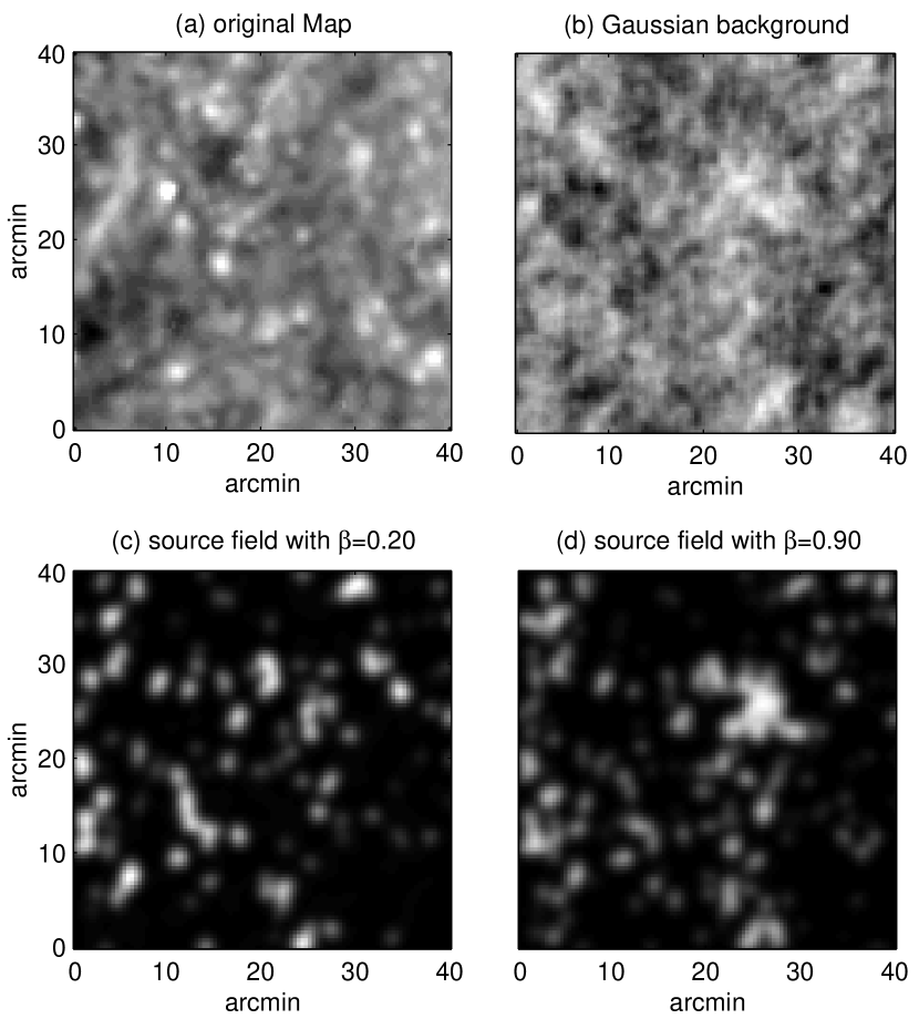
Figure 3: Panel (a) shows the original ISO far-IR map. The simulated Gaussian background map obtained via Fourier phase randomization is shown in (b). Panels (c) and (d) show simulated source fields for $\alpha=0.20$ and $\alpha=0.90$, respectively.

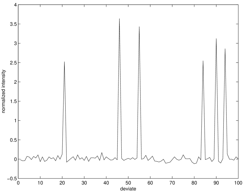
Figure 4: One-dimensional realization of a sequence of uncorrelated deviates from the two-component Gaussian mixture used for Figure 3 (see text). The intensity was based on the ISO map normalized to unit standard deviation.

References

- Avelino et al. (1998) Avelino, P.P., Shellard, E.P.S., Wu, J.H.P. & Allen, B. 1998, ApJ, 507, L101
- Diggle (1983) Diggle, P.J 1983, Statistical Analysis of Spatial Point Patterns (London: Academic Press)
- Dilts (1985) Dilts, G. A. 1985, Journal of Computational Physics, 57, 439
- Dole, et al. (2001) Dole, H., et al. 2001, A&A, 372, 364
- Driscoll & Healy (1994) Driscoll, J. R. & Healy, D. 1994, Adv. in Appl. Math., 15, 202
- Kessler et al. (1996) Kessler, M.F., et al. 1996, A&A, 315, L27
- Le, Martin & Raftery (1996) Le, N. D., Martin, D. & Raftery, A. E. 1996, Journal of the American Statistical Association, 91, 1504
- Lemke, Klaas & Abolins (1996) Lemke, D, Klaas, U. & Abolins, J. 1996, A&A, 316, L64
- Maino et al., (2001) Maino D., et al. 2001, MNRAS, submitted (astro-ph/0108362)
- Mandolesi et al., (1998) Mandolesi N., et al. 1998, Planck Low Frequency Instrument, a proposal submitted to ESA
- Martinez & Saar (2001) Martinez, V.J. & Saar, E. 2001, Statistics of the Galaxy Distribution (New York: Chapman & Hall)
- McLachlan & Peel (2000) McLachlan, G. & Peel, D.A. 2000, Finite Mixture Models (New York: Wiley)
- Mo & White (1996) Mo, H.J. & White, S.D.M. 1996, MNRAS, 282, 347
- Ogorodnikov & Prigarin (1996) Ogorodnikov, V.A. & Prigarin, S.M. 1996, Numerical Modelling of Random Processes and Fields: Algorithms and Applications (Utrecht: VSP)
- Peebles (1999) Peebles, P.J.E. 1999, ApJ, 510, 531
- Pilbratt (2001) Pilbratt, G. 2001, The FIRST ESA Cornerstone Mission, in IAU Symp. 204, The Extragalactic Infrared Background and its Cosmological Implications, August 2000 Manchester, eds. M. Harwit & M.G. Hauser (San Francisco: ASP), 39
- Popescu, Deodatis & Prevost (1998) Popescu, R., Deodatis, G. & Prevost, H. 1998, Prob. Engng. Mech., 13, 1
- Priestley (1981) Priestley, M.B. 1981, Spectral Analysis and Time Series (London: Academic Press)
- Puget et al., (1998) Puget, J.L., et al. 1998, High Frequency Instrument for the Planck Mission, a proposal submitted to ESA
- Ruan & McLaughlin (1998) Ruan, F. & McLaughlin, D. 1998, Advances in Water Resources, 21, 385