Cosmological Parameters, Dark Energy and Large Scale Structure

Abstract

We review the current status of cosmological parameters, dark energy and large-scale structure, from a theoretical and observational perspective. We first present the basic cosmological parameters and discuss how they are measured with different observational techniques. We then describe the recent evidence for dark energy from Type Ia supernovae. Dynamical models of the dark energy, quintessence, are then described, as well as how they relate to theories of gravity and particle physics. The basic theory of structure formation via gravitational instability is then reviewed. Finally, we describe new observational probes of the large-structure of the universe, and how they constrain cosmological parameters.

I Introduction

In what is now a classic story, lies the foundation of 21st century cosmology. In 1917 Einstein formulated the field equations which suggested a dynamic universe, in contradiction to the available data which supported a static universe. Einstein thus added his now famous “fudge factor”, the cosmological constant. Following Edwin Hubble’s 1926 paper in which he suggested an expanding universe, Einstein removed the cosmological constant. The subsequent history of cosmology has leapfrogged between experiments to measure the cosmological parameters (expansion rate, mass density, deceleration rate, geometry and now energy density) and theories to organize them.

However, the last few years have been very exciting for cosmologists. Cosmic microwave background experiments, observations of Type Ia supernovae, large scale surveys of galaxies and clusters and the Hubble key project have yielded unhitherto precise measurements of the key cosmological parameters. Furthermore, these new values have provided a concordance model, a flat universe with a significant component of “dark energy” which accelerates the expansion in the current epoch, which challenges our fundamental theories of particle physics.

In this report, we summarize the current status of the cosmological parameters (the Hubble constant, mass and vacuum energy density (dark energy)), quintessence and large scale structure; and their import on modern cosmology.

II Cosmological Parameters: The Hubble Constant

The Hubble constant is a fundamental parameter of modern cosmology but its value has remained very uncertain despite many experiments which claimed small errors. Recently, a major effort to use the Hubble Space Telescope (HST) to measure Cepheid variable stars in galaxies well beyond the local group was completed by the Distance Scale Key Project and has yielded a value of $72\pm 7$ km s^-1 freedman2001 . This comprehensive study used a number of tertiary distance indicators, such as Tully-Fisher and Type Ia supernovae (SNIa) to reach the Hubble flow with consistent results. The value of 72 km s^-1 is also in accordance with an independent method employing surface brightness fluctuations of galaxies ajhar . Still, there remains another group using Cepheids with HST which continues to obtain a significantly lower value of $59\pm 6$ km s^-1 parodi .

The top of the distance ladder appears to be more secure than the middle or bottom rungs. From studies in the Hubble flow ($0.01<z<0.1$), the peak brightness of SNIa appear to be a function of a single parameter characterized by their light curve shape phillips . SNIa can provide a distance good to 7% to any galaxy that has a well-observed SNIa. And this technique can be extended to ’peculiar’ SNIa, thus removing the need for selection criteria that might induce systematic error garnavich . The major sources of uncertainty in the Hubble constant are currently the unknown effect of metallicity variations on the Cepheid period-luminosity relation and the continuing debate on the distance to the Large Magellanic Cloud (jha ).

Other methods to determine the Hubble constant such as applying the Sunyaev-Zeldovich effect to galaxy clusters (mason ) or using the time delays in gravitational lens images (williams ) show promise but are currently limited by large systematic uncertainties.

III Cosmological Parameters: Dark Energy

III.1 Type Ia Supernovae and the discovery of the Dark Energy

Type Ia supernovae (SNe Ia) are very bright, calibratable standard candles. Upon explosion they release some 10⁵¹ ergs, outshining a typical galaxy. This makes them ideal tools for cosmology since they can be detected to high redshifts. The actual measurements are fundamentally straightforward: brightness and redshift. The former is obtained with imaging data, and the latter from spectroscopy. The relationship between the observed apparent brightness and the redshift of standard candles depends on the cosmological parameters mass density, vacuum energy density and curvature.

Two groups, the Supernova Cosmology Project (SCP) and the High Z Team (HZT) have programs to observe high redshift SNe at $z>0.3$. To date the SCP and the HZT have together discovered over 100 SNe Ia. In 1998 both teams independently announced their results of an accelerating universe, suggesting the presence of a vacuum energy or dark energy component to the total mass-energy budget(perlmutteretal1999 , riessetal1998 .

The standard method pioneered by the SCP for discovering high redshift SNe ’on demand’, requires two epochs of observations spaced about 3 weeks apart, just after and just before consecutive new moons on a 4m or larger class telescope. This cadence allows the discovery of a batch of SNe before they reach maximum brightness, and, importantly, enables spectroscopic and photometric follow up with scheduled observations. Supernova type is confirmed and redshift determined for each candidate SNe with spectroscopy at peak brightness obtained with large aperture telescopes, e.g. Keck I and II, the VLT. Follow up photometry at regular intervals are obtained for a period of roughly 60 days around peak to determine the light curve shape in order to normalize the peak magnitude by correcting for the brightness-light curve width relation (see Fig. 1).

Figure 1: Top panel: lightcurves for low redshift type Ia supernovae from the Calan-Tololo Survey showingthe diversity in brightness and light curve width. Bottom panel: the same SN lightcurves after correcting for the magnitude-width (empirical) relation by ”stretching” the time axis. They now lie on the same curve.

Once the peak brightness has been determined, the supernovae are plotted on a Hubble diagram (brightness vs. redshift) as in Fig. 2. Redshift is a measurement of the expansion since light left the SN and brightness is a measure of the time since light left the SN. Shown in Figure 2 are a sample of fully analyzed distant ($z>0.3$) Type Ia supernovae from the HZT and SCP as well as a sample of nearby ($z<0.1$) SNe Ia from the Calan-Tololo Survey. Superposed are three cosmological models, the standard model ($\Omega_{M}=1$, no cosmological constant), an open model ($\Omega_{M}=0$, $\Lambda=0$) and a $\Lambda$ model ($\Omega_{M}$, $\Lambda>0$). The SNe data favor a cosmology with low matter density and a cosmological constant, $\Lambda$, or dark energy model.

Figure 2: Top panel: The Hubble diagram for type Ia supernovae combining data from the Calan-Tololo Survey (red) and CfA Supernovae (blue) at low $z$ and the SCP (red) and HZT (blue) at high redshift. Three possible cosmologies are shown with lines. A flat, matter dominated universe is the dashed line, an open, matter dominated cosmology as a dotted line and a flat, cosmological constant dominated universe is indicated by a solid line. Bottom panel: same as the top panel but with the open, matter dominated universe subtracted from the data. A lambda dominated universe is clearly favored by both research group’s results.

These data can be jointly fit for mass density and vacuum energy density (cf. goobarperlmutter ). Figure 3 shows the confidence region (in blue) of the joint fit for SCP supernovae, yielding a ”best” value of $\Omega_{M}\sim~{}0.3$, and $\Omega_{\Lambda}\sim~{}0.7$ (perlmutteretal1999 ). The HZT also obtained similar results (riessetal1998 ). Drawn in this figure are the confidence regions from the CMB (MAXIMA, Boomerang) experiments ( langeetal , balbietal ) - perpendicular to that of the SNe, and from cluster counting programs (for example, bahcalletal1999 ). The supernovae evidence for a vacuum energy density is in remarkable concordance with the galaxy cluster measurements (sensitive only to the value of $\Omega_{M}$) (bahcalletal1999 ), and the recent Cosmic Microwave Background results (e.g Maxima, Boomerang) which are sensitive to curvature, $\Omega_{\kappa}$ (langeetal , balbietal ).

Figure 3: The two-parameter joint fit confidence regions for the vacuum energy density and mass density. The oval contours (upper left) are the fit for a sample of high redshift type Ia supernovae. The results from the recent cosmic microwave balloon experiments lie along the flat universe line, perpendicular to the SNe contours. Also included are the confidence regions for various cluster counting methods, which are insensitive to $\Lambda$.

It is this result that leads to a surprising conclusion. The Universe’s expansion is accelerating rather than merely decelerating as would be expected due to gravity alone. This means that the standard cosmology model - matter dominated, flat universe – appears to be wrong, leading to the conclusion that our understanding of fundamental physics is incomplete. We are left with primary questions: What is the nature of the vacuum energy density that accelerates the expansion? When was the “era of deceleration”? What is the history of expansion of the universe?

One approach to investigating the nature of this new energy component is to determine its equation of state. A cosmological constant has an equation of state $w=p/{\rho}=-1$. If this vacuum energy is due to some other primordial field, e.g quintessence (see discussion below) or cosmic defects its dynamical properties would be very different from a cosmological constant. In Figure 4, we show the best fit confidence regions from the supernova work in the $\Omega_{M}$ - $w$ plane for a vacuum energy density whose equation of state is $w=p/{\rho}$, constrained to a flat universe. The value for $\Omega_{M}$ is between 0.2 and 0.4, and $w<-0.33$ (cf. perlmutteretal1998 , garnavichetal1998 ). Also shown are the regions covered by quintessence tracker modesl (e.g. albrecht ), cosmic strings and a cosmological constant ($w=-1$). The small (yellow) area within the current SN confidence regions is the expected confidence region allowed by the proposed SNAP satellite observations for $w=-1$ and $\Omega_{M}=0.28$.

III.2 The Future: Dark Energy Parameters and SNe Ia

A proposed experiment to achieve the precision required to determine the values of the cosmological parameters and investigate the dark energy properties is with SNAP’s (Supernova Acceleration Probe) supernova program (snowmass2001 ). By exploiting and extending the brightness-redshift relation of SNe Ia to higher redshifts, we can probe the era of deceleration as well as measure the actual magnitude of the values for $\Omega_{M}$ and of $\Omega_{DE}$. Increasing the number of discovered and studied SNe Ia to $\sim$ 2500 per year, out to redshifts of $z=1.7$, will enable this technique to identify and limit systematic errors while satisfying the statistical requirements. The recent results of SN 1997ff, a SN Ia discovered in the Hubble Deep Field (riessetal2001 ) demonstrates the power of this kind of experiment. With such a dataset, $\Omega_{M}$ and $\Omega_{DE}$ can be determined to a few percent and models for the vacuum energy tested (Figure 4). Perhaps then the missing energy problem may be understood.

Figure 4: In this figure we show the confidence region for high redshift supernovae in the $w$–$\Omega{M}$ plane for a flat universe with constant $w$, where $w$ is the equation of state parameter. Also shown are the regions predicted by cosmic strings (at $w=1/3$), by a range of quintessence models ($-0.8<w<-0.3$) and by a cosmological constant ($w=-1$).

III.3 The Missing Energy Problem

The total energy density of the Universe is much greater than the energy density contributed by all baryons, neutrinos, photons, and dark matter. Deepening this mystery are the recent observations of type Ia supernovae which suggest that the expansion rate of the Universe is accelerating. One possible resolution is a cosmological constant which fills this energy gap.

The existence of a cosmological constant, $\Lambda$, at an energy density $\sim 120$ orders of magnitude below reasonable estimates presents a distinct challenge to fundamental physics. Adding to the challenge is the apparent coincidence (in cosmological scales) in the present-day amplitude of the missing energy, dark matter, baryon, and radiation densities. If there is a significance to this multiple coincidence, then we may suspect that there is some mechanism responsible (not unlike supersymmetry, which is theorized to pull together the gauge couplings in a triple “coincidence”). This provides some motivation to consider a dynamical component for the missing energy. Hence, a logical alternative to the cosmological constant is “quintessence,” a time-dependent, spatially inhomogeneous, negative pressure energy component which drives the cosmic expansion. (See Ratra:1988rm ; Peebles:1988ek ; Frieman:1995pm ; Coble:1997te ; Caldwell:1998ii .)

IV Quintessence

Quintessence (Q) is a time-varying, spatially-inhomogeneous, negative pressure component of the cosmic fluid. It is distinct from $\Lambda$ in that it is dynamic: the Q energy density and pressure vary with time and is spatially inhomogeneous. A typical example of quintessence is a scalar field slowly rolling down a potential, similar to the inflaton in inflationary cosmology. Unlike $\Lambda$, the dynamical field can support long wavelength fluctuations which leave an imprint on the CMB and the large scale distribution of matter. Another, critical distinction is that $w$, the ratio of the pressure ($p$) to the energy density ($\rho$), is $-1<w\leq 0$ for quintessence, whereas $w$ is precisely $-1$ for $\Lambda$. Hence, the expansion history of the Universe for $\Lambda$ and Q models are different. There is much rich behavior to explore in a cosmological model with quintessence. (See Wang:2000fa for an exhaustive survey of cosmological phenomena impacted by quintessence.)

Fundamental physics, e.g. those theories of gravity and fundamental interactions beyond the standard model of particle physics, provide some motivation for light scalar fields, one of which may serve as a cosmic Q field. In this way, quintessence serves as a bridge between the fundamental theory of nature and the observable structure of the Universe.

In the following, we identify the cosmological parameters which describe the dark energy in the framework of the quintessence scenario. In discussing these parameters, we have a mind towards both observation and the interpretation in terms of the underlying physics.

IV.1 Background Parameters: $\Omega$ and $w$

The existence, and in fact dominance, of dark energy in the Universe is characterized by $\Omega_{Q}$, the energy fraction. While a broad range of observational evidence indicates a low matter density fraction, $\Omega_{m}<1$, the existence of dark energy does not obviously follow. That the missing energy is filled by something, rather than nothing (perhaps curvature), is deduced after the critical cosmic microwave background measurement of the geometry of the Universe, and hence, $\Omega_{Q}\approx 1-\Omega_{m}$. The present best limits on the dominating dark energy density give

$$\Omega_{Q}\approx 0.7$$

with typical $1\sigma$ uncertainties of $\pm 0.1$, which grow when certain assumptions are relaxed (e.g. assuming flatness, $h$, $\Lambda$). (See Bahcall:1999xn and BOOMresults .) Because the dark energy does not cluster significantly (at least on scales $\lesssim 50$ Mpc), we cannot assess its energy density in the same ways that we tally up the mass density of stars or galaxies. Nevertheless, because of the widespread role of the dark energy density, numerous observations can help pin down this number. For example, type 1a supernovae magnitudes, galaxy counts, the CMB, and strong gravitational lens optics all have in common a dependence on the relationship between luminosity distance and redshift,

$$d_{L}(z)={c\over H_{0}}(1+z)\int_{0}^{z}\,dz^{\prime}/\sqrt{(1+z^{\prime})^{3}\,\Omega_{m}+\Omega_{Q}[z^{\prime}]}.$$

(Other distance have different weights in redshift— the differences are not important here, which is actually a disadvantage in measuring $w$ Maor:2001jy .) Assuming a simultaneous measurement of the Hubble constant, we see that distance measurements are sensitive to the dark energy density over a range of redshift. We also see that characterizing the dark energy density by a single parameter, $\Omega_{Q}$ at $z=0$, only makes sense if the energy density is slowly varying over the interval observed.

To construct a cosmological model, we must know the time evolution of the dark energy density. Theory has offered up a variety of ideas, yet rather than get bogged down in the details of one particular model (and which one to choose?), a reasonable first step is to encode the time evolution in the equation of state, $w$, defined as the ratio of the pressure to the energy density of the homogeneous dark energy. A given time history for $w$ can be used to determine the history of the energy density,

$$\rho_{Q}(a)=\Omega_{Q}\rho_{crit}\exp{\left(3\int_{a}^{1}[1+w(a^{\prime})]\,d\ln a^{\prime}\right)},$$

where $\Omega_{Q}$ is the energy fraction at the present, when $a=1$ is the scale factor. For a cosmological constant, $w=-1$ for all times, and the energy density is a constant. Whereas for a scalar field evolving in a potential, the field equations of motion must be solved in order to follow the pressure and energy density, a time history for $w$ can suffice, and in fact implies a potential and field amplitude, given by the parametric equations

$$V(a) = \frac{1}{2}[1-w(a)]\rho_{Q}(a)$$ (1)

$$Q(a) = \int da^{\prime}{\sqrt{1+w(a^{\prime})}\over a^{\prime}H(a^{\prime})}\sqrt{\rho_{Q}(a^{\prime})}.$$

Reconstruction of a continuous function such as the potential from observations of the expansion history is an unrealistic goal, considering systematic uncertainties. But this equivalence between the equation of state and the potential, $w(a)\leftrightarrow V(Q[a])$, immensely simplifies the study of quintessence. It means a theorist can forgo details such as masses and exponents when comparing with observation, and observers need only interpret phenomena in terms of an average $w$ over a range of red shift. This average,

$${\Large\bar{w}}=\int da\,\Omega_{Q}(a)w(a)\,\,/\int da\,\Omega_{Q}(a)$$

is the second parameter which we require to characterize quintessence or dark energy. The best $2\sigma$ limit on the equation of state gives

$${\Large\bar{w}}\lesssim-0.5$$

based on a conservative interpretation of the current data Wang:2000fa ; Garnavich:1998th ; Perlmutter:1999jt ; Efstathiou:1999tm .

Introducing ${\Large\bar{w}}$ enlarges our cosmological parameter space, and reduces the sharpness of existing measurements of the other parameters. It is important to realize that theoretical models of quintessence are not evenly distributed in “$w$-space.” This should be taken as a warning to all those statisticians desiring to marginalize over $w$ (a theorist’s prior is inhomogeneous at best!). Furthermore, the physical, observable difference between two cosmological models with a fixed difference in $w$, $\Delta w$, is not uniform throughout “$w$-space.” For example, using the CMB as a discriminant, the difference between $w=-1$ and $w=-0.9$ cosmologies is much smaller than the difference between $w=-0.6$ and $w=-0.5$. An alternate description of the effect of the dark energy on the cosmic expansion may be made with the red shift at which the quintessence and matter densities were equal, $z_{QM}$, or the red shift at which acceleration began, $z_{ACC}$. These red shifts can be used to describe the change of behaviour in, say, the growth rate of matter density perturbations or the accumulation of the integrated Sachs-Wolfe effect in the CMB. Investigations of various methods to measure $w$ include Newman:1999cg ; Huterer:2000mj ; Haiman:2000bw . Probably the most ambitious, focused method for attacking the dark energy, with the potential for dramatic results, is the Supernova Acceleration Probe, or SNAP (see snap.lbl.gov and elsewhere in these proceedings).

It is useful to make some comments on $w$ in the context of quintessence. Among the field theory models proposed, few predict a constant equation of state when the cosmic scalar field comes to drive the expansion rate. Technically, the change in the Hubble damping term pushes the field into a transient regime which, because the Universe is not completely Q-dominated, still persists today. However, for a slowly evolving field, $\dot{w}\lesssim H$, the average ${\Large\bar{w}}$ is not too different from the range of values sampled by $w(a)$ over the last Hubble time. On the other hand, models have been proposed which feature an oscillating field in which case averaging smooths out rapid oscillations ($\dot{w}\gg H$) and ${\Large\bar{w}}$ describes the slow drift in the pressure which drives the accelerating expansion.

What will measurement of $w$ tell about the theory? In the case ${\Large\bar{w}}\approx-1$ it will be impossible to discriminate between whether the dark energy is a true cosmological constant or just a very slowly evolving field, unless there exist nonlinear excitations of the $Q$ field. If ${\Large\bar{w}}\lesssim-0.7$ we can conclude that the dark energy is not a quintessence tracker field Steinhardt:1999nw . If a measurement of ${\Large\bar{w}}$ at an earlier red shift interval is made, then we could infer the sign of the derivative, $\dot{\Large\bar{w}}$. If $\dot{\Large\bar{w}}<0$ the equation of state is becoming more negative, driving greater acceleration; this is a common feature of slowly rolling fields, especially trackers Zlatev:1999tr . If $\dot{\Large\bar{w}}>0$ the equation of state is becoming less negative, suggesting the period of acceleration is temporary, a coasting stage. Any of these results would have a tremendous impact on theory.

The lower bound on $w$ is often taken to be $-1$, the limiting case of a cosmological constant. However, there is no strict prohibition on a more negative equation of state, $w<-1$. Certainly, a canonical, homogeneous scalar field in Einstein gravity cannot achieve such super-negative pressure, and violation of certain of the energy conditions ($\rho+p<0$ with $\rho>0$ violates the dominant energy condition) may signal unusual physics. Indeed, toy models of quintessence have been constructed which have a super-negative equation of state Caldwell:1999ew . However, the interpretation of observation and experiment should not be constrained by these considerations. After all, nature may be trying to tell us something.

IV.2 Perturbative Parameters: $\lambda$ and $c$

A time-evolving dark energy component must necessarily fluctuate in response to inhomogeneities in the surrounding matter distribution. Hence, we can expect there to be fluctuations in the quintessence which leave an imprint on the large scale distribution of matter and the cosmic microwave background. Detection of these fluctuations would reveal information about the microphysics of the dark energy.

The microphysical model describes the behavior of density and pressure fluctuations, and any other properties of the dark energy. This is information not contained in the equation of state, which merely reflects the gross features of the medium. Nor is this information contained in the formal theory of cosmological perturbations, which provides evolution equations for certain geometric quantities. What we require is a description of excitations in the dark energy, giving the relationship between $\delta P$ and $\delta\rho$ as a function of time and length scale. In general, this requires a continuous function of two variables for the speed of propagation of statistically homogeneous perturbations in the dark energy, $c_{s}^{2}(t,\vec{x})=\delta P/\delta\rho$. As a simplification, we introduce two new cosmological parameters, $\lambda_{Q}$ and $c_{Q}$ which may be approximately understood as $c_{s}=1$ for $\lambda<\lambda_{Q}$ and $c_{s}=c_{Q}$ for $\lambda>\lambda_{Q}$.

In the case of quintessence, the microphysical model is determined by the Lagrangian density

$$L=\frac{1}{2}\partial_{\mu}Q\,\partial^{\mu}Q-V(Q)$$

for the cosmic scalar field $Q$ with a potential $V(Q)$. Fluctuations $\delta Q$ about the homogeneous background field $Q$ obey the wave equation

$$\delta Q^{\prime\prime}+2{a^{\prime}\over a}\delta Q^{\prime}+\left(V_{,QQ}-\nabla^{2}\right)\delta Q=-{1\over 2}h^{\prime}Q^{\prime}$$

from which the solution is used to construct quantities such as the energy density, which is linear in $\delta Q,\,\delta Q^{\prime}$. Here, $h$ is the trace of the synchronous gauge metric perturbation, and for practical purposes is proportional to the time derivative of the matter density contrast. So we can see that the quintessence reacts to the external gravitational field through $h$. The nature of the response is determined by $V_{,QQ}$, which characterizes the effective mass of the scalar field, $m_{Q}=\sqrt{V_{,QQ}}$. The speed of propagation of the perturbations is $c_{Q}=1$, so that the characteristic perturbation length scale is $\lambda_{Q}=1/\sqrt{V_{,QQ}}$. Taking advantage of the equivalence between the equation of state and potential for the scalar field, one can express $V_{,QQ}$ in terms of $a,\,w$ and time-derivatives thereof. For a slowly evolving field, it turns out that $V_{,QQ}\propto H^{2}$, meaning that fluctuations $\delta Q$ on scales smaller than the Hubble scale dissipate, keeping the field smooth, non-clustering. On larger scales, the field is unstable to gravitational collapse and long wavelength perturbations develop. These perturbations leave an imprint on the large scale distribution of matter.

There are variations on the basic quintessence model which describe the same background, characterized by parameters $\Omega_{Q}$ and $w$, but have very different microphysics and in turn, different clustering properties. One example is k-essence Armendariz-Picon:2000dh ; Armendariz-Picon:2001ah , a scalar field with a non-canonical kinetic term in the Lagrangian, for which the sound speed can be small, $c_{Q}\ll 1$, allowing for pressureless fluctuations to collapse via gravitational instability. Another example is a rapidly oscillating field, for which $\dot{w}$ can be much larger than $H$, in which case the clustering scale can be much smaller that the Hubble length, $\lambda_{Q}\ll H^{-1}$, while keeping ${\Large\bar{w}}$ sufficiently negative to drive the accelerated expansion Sahni:2000qe ; Dodelson:2000fq .

The best shot at detecting the long wavelength fluctuations predicted in quintessence models is to use full sky maps that trace cosmic structure on the largest scales. Cross-correlation of different tracers, such as the CMB and weak lensing, can be used to isolate the unique features of quintessence. (See the discussion in Caldwell:2000wt .) This may be difficult, however, since large scale phenomena is fundamentally limited by cosmic variance, not to mention systematic uncertainties. Yet the payoff would be worth it. Detection of dark energy clustering at lengths below the Hubble scale would provide an important clue to the physics of dark energy, indicating a solution different from the cosmological constant.

IV.3 Circumstantial Evidence: $\dot{G}/G$ and $\dot{\alpha}/\alpha$

Detection of a slow drift in the value of the gravitational Newton’s constant, or the electromagnetic fine structure constant, would indicate radical new physics well outside the confines of conventional theory. Such a result might also be a signal for an evolving cosmic scalar field: scalar fields which modulate the strength of coupling constants appear frequently in the same models of high energy physics which motivate models of quintessence. With a coupling to the gravitational or electromagnetic action, such scalar-tensor or scalar-vector theories with a flat potential could also provide the dark energy. (See Amendola:2000er ; Baccigalupi:2000je and references therein.) Because constraints on the evolution of such constants are so tight (see Carroll:1998zi for a review in the quintessential context), the quintessence coupling must be relatively insensitive to the field evolution, or the field $Q$ must be very slowly creeping down the potential. Just the sort of behavior needed for negative pressure.

IV.4 Dark Energy Summary

Provided that the trend in the observational data continues, we will find ourselves with strengthening evidence for the missing energy problem. How do we then proceed?

The first order of business is to refine the measurements of the basic cosmological parameters. That is, we must verify that the matter density is low, $\Omega_{m}<1$, that the spatial curvature is negligible, $|\Omega_{k}|\ll 1$, and that there is indeed a missing energy problem. Since most phenomena are sensitive to a combination of cosmological parameters, the measurement of the Hubble constant must also be further refined.

Given that the missing energy problem is real, the next logical step will be to characterize the equation of state, $w$, in order to determine whether the dark energy is $\Lambda$, $Q$, or other. For fundamental physics, $\Lambda$ and $Q$ represent new, ultra-low energy phenomena beyond the standard model. If firmly established by observations and experiment, the discovery will go down in history as one of the greatest clues to an ultimate theory.

Once the basic properties of the dark energy are determined, $\Omega_{Q}$ and $w$, we can begin to ask questions about the microphysics — what is it? Long wavelength fluctuations, manifest in very large scale structure and the CMB are potential clues.

Finally, the structure of our cosmological models, the missing energy problem and the quintessence hypothesis, are predicated on the validity of Einstein’s GR, and the existence of cold dark matter supporting a spectrum of primordial, adiabatic density fluctuations. It is critical that we test this framework at the same time that we look for the dark energy.

V Large Scale Structure: Theory

Large scale structure can constrain the cosmological parameters, through the effect of density fluctuations. It is impossible to do justice to the vast field of large scale structure studies in a few pages in this report. Instead, we choose to focus on two issues: how secure is the gravitational instability paradigm for structure formation? and what does large scale structure teach us about particle physics? emphasizing a review of the conceptual issues rather than detailed quantitative estimates and measurement. We will also discuss several new techniques/observational windows in the context of the first question. (Traditionally, the term large scale structure is reserved for the study of the large scale distribution of mass as manifested through galaxies. Here, we use it to include other tracers as well). We refer the reader to excellent reviews in peebles80 ; roman01 for more discussions.

V.1 The Gravitational Instability Paradigm

The most successful and the most thoroughly studied theory of structure formation postulates that the observed large scale structure, as manifested through galaxies, clusters, weak gravitational lensing as well as quasar absorption, arise from the growth of fluctuations under gravity textbooks . A common and necessary ingredient of such a theory is the presence of a large amount of dark matter which interacts very weakly except through gravity. How successful is this theory?

Tests of this theory can be roughly divided into three categories. As we will see, none of them offer a completely clean test, but together they form a compelling, though far from air-tight, argument in favor of gravitational instability.

V.1.1 The Clustering Hierarchy

Assuming Gaussian initial conditions (such as predicted or at least preferred by inflation), gravity predicts a definite hierarchy of correlations where $\xi_{N}\propto{\xi_{2}}^{N-1}$ where $\xi_{N}$ is the N-point correlation function of the mass peebles80 ; fry ; davis . The proportionality constant can be robustly predicted on large scales using perturbation theory bernardeau . Such a hierarchy (including the predicted proportionality constant) appears to be consistent with the observed galaxy correlations enrique ; istvan ; enriquelam ; romantrispec . However, one uncertainty remains in the interpretation: the relation between mass and galaxy, the bias. To take a simple example, suppose the fluctuation in galaxy density ($\delta_{g}=(n_{g}-\bar{n}_{g})/\bar{n}_{g}$, where $n_{g}$ is the galaxy density and $\bar{n}_{g}$ its mean) is related to the fluctuation in mass density ($\delta=(\rho-\bar{\rho})/\bar{\rho}$) via:

$$\delta_{g}=b\delta$$ (2)

where $b$ is the bias factor (see fryenrique ; mowhite ; pendekel for more general biasing schemes). Then, the observed galaxy skewness, which relates the spherically averaged three-point function to the averaged two-point function i.e. $S^{g}_{3}\equiv\langle\delta_{g}^{3}\rangle/\langle\delta_{g}^{2}\rangle^{2}$ is given by

$$S^{g}_{3}=S_{3}/b$$ (3)

where $S_{3}$ is the mass skewness, defined by $S_{3}\equiv\langle\delta^{3}\rangle/\langle\delta^{2}\rangle^{2}$. Inference of the mass hierarchical constants (such as $S_{3}$), which is predicted by theory, from the observed galaxy distribution therefore depends on assumption about how galaxy traces mass. What is perhaps surprising is that the theoretically predicted $S_{3}$ (analogous higher order quantities) does appear to agree with the inferred $S_{3}$ if bias is assumed to be, $b\sim 1$ enrique ; istvan .

That gravitational instability, together with the simplest but by no means obvious assumption that galaxies trace mass, can readily explain the observed hierarchy should be counted as one successes of the theory. However,the interpretation is somewhat complicated by the issue of bias. Workers in the field have turned the argument around: assuming gravitational instability, use the observed hierarchy to constrain bias frytrispec ; romantrispec . See also steidel for evidence that bias is non-trivial at high redshifts ($z\sim 3$), and frybias ; maxpeebles for discussions of how bias might evolve under simple assumptions.

V.1.2 Velocities

Another robust prediction of gravitational instability is the relation between density and velocity. Conservation of mass tells us bertschinger :

$${\partial\delta/\partial\tau}=-\nabla\cdot v$$ (4)

where we have kept terms to first order (i.e. $\delta$ and peculiar velocity $v$ are both small), and $\tau$ is the conformal time. According to linear perturbation theory, the fluctuation $\delta$ grows as $\delta\propto D(\tau)$ where $D(\tau)$ is the growth factor dictated by gravity. Hence the above equation can be rewritten as

$$\delta=-({D/D^{\prime}})\nabla\cdot v$$ (5)

where ^′ denotes derivative with respect to $\tau$. Such a simple relation between overdensity and peculiar velocity can be tested, using galaxies as test particles. There are many ways to do so, but they fall roughly into two classes. The first makes direct use of peculiar velocities measured in surveys to reconstruct the density field, which is then compared with the observed density field or vice versa potent ; dekelpotent . This approach requires accurate distance indicators, however. The commonly used Tully-Fisher method gives error-bars that are somewhat large; independent, more reliable methods would be desirable riessvel ; SBF The second makes use of the fact that peculiar velocities introduce a systematic distortion of the galaxy density field and its correlations in the observed redshift-space kaiser ; fisher ; hamilton . resulting in a systematic line-of-sight-squashing of the correlation function on large scales kaiser .

Much research has been carried out following the above two approaches. The quantitative success of these tests depends on two additional parameters: 1. $\Omega_{m}$ (the matter density in units of the critical density) which largely determines the growth rate $D$, and 2. the bias $b$, because, as before, galaxy density is observed instead of the mass density. Indeed, very often, the problem is turned around: instead of testing gravitational instability, one assumes it and uses the above to measure $\Omega_{m}$ and $b$ or some combination of them. The fact that such measurements yield values for $\Omega_{m}\sim 0.3$ and $b\sim 1$ velocityrecent ; zrecent , which are consistent with other independent measurements (see other sections in this report), should be counted as another success of the theory. However, it remains to be seen whether improving accuracy will reveal inconsistency.

V.1.3 Fluctuation Growth

The rate at which fluctuations grow via gravitational instability, from the epoch of recombination (probed by the microwave background) to the present, can be predicted precisely provided we know the amount of dark matter, the nature of dark matter (whether it is hot or cold), the primordial power spectrum (particularly its scale dependence), and so on. Gravitational instability plays the role of bridging the gap between information from early epochs to late epochs. As such, microwave background and large scale structure data test gravitational instability only to the extent that some of the parameters can be independently constrained, or have values that are strongly motivated by theory (i.e. inflation). Indeed, the combination of microwave background and large scale structure, the latter as measured from surveys of present day galaxies, has provided a wealth of constraints on several cosmological parameters boompapers .

Methods of measuring fluctuation growth include measuring the galaxy correlation as a function of redshift (though growth can be confused with bias evolution) and counting of the number density of clusters as a function of redshift. Clusters as rare events probe the tail of the fluctuation probability, and provide a sensitive measure of the amplitude of the power spectrum and its evolution (the latter determined by $D(\tau)$ and hence by $\Omega_{m}$) clusters . It is also a useful diagnostic of non-Gaussianity in the initial fluctuations clustergauss . The Lyman-alpha forest or weak gravitational lensing can be used to more directly measure the evolution of mass clustering. What is impressive about the results using these methods is that the simplest assumptions about the various components seem to hold up well e.g. cold dark matter with a scale invariant power spectrum of adiabatic, Gaussian fluctuations in a flat universe – together with growth via gravitational instability. The major surprise in this picture is the need for a cosmological constant or some form of dark energy, as independently confirmed by supernovea measurements SN . Expected improvements in precision will severely test this paradigm baryon .

V.1.4 A Note on Galaxy Formation

The growth of fluctuations with a power spectrum $P(k)\sim k^{n}$, where $n>-3$ and $k$ is the wavenumber, leads to a generic prediction: small objects go nonlinear first as one marches forward in time. This is easy to see: the root-mean-squared amplitude of the mass fluctuation at a given wavelength $\lambda=2\pi/k$ behaves as:

$$\sqrt{\langle|\delta_{k}|^{2}\rangle}\sim\sqrt{k^{3}P(k)}\propto D(t)k^{(3+n)/2}$$ (6)

where $\delta_{k}$ is a Fourier mode, and $D(t)$ is the fluctuation growth rate. Clearly, if $n>-3$, wavemodes with a high $k$ or small wavelength go nonlinear first. This leads to a picture of heirarchical galaxy formation in which small objects collapse first and then subsequently merge to form larger nonlinear objects. As dark matter collapses, gas accretes and is shocked, eventually cooling to to form stars and galaxies whiterees . The theory of hierarchical galaxy formation has developed into a major industry whitereview . Because of the inherently complex gas physics, robust and precise predictions are hard to come by, except on large scales where it is believed that a simple linear bias (eq. 2) suffices to describe the galaxy two-point correlations (a generalization of the linear bias into a power series is needed to describe the higher order correlations; see fryenrique ). The most tractable part of the problem: namely, the formation and merging of dark matter halos, has been very successfully solved by both numerical N-body simulations edNbody and analytic excursion set theory excursion . Recently, there has been some excitement over the development of a formalism that parametrizes in an economic way our ignorance of the detailed gas physics, and allows us to make progress towards linking small-scale clustering to galaxy formation physics halomodel . The search for robust predictions from the hierarchical galaxy formation theory remains an important goal. For possible problems with this theory, see peebles .

V.2 The Particle Physics Connection

One of the main goals of large scale structure studies is to discover the nature of the density fluctuations in the early universe. This is where large scale structure and particle physics meet. At present, the most comprehensive and successful theory of the initial conditions of the universe is inflation inflation . The simplest models of inflation predict a spectrum of nearly scale invariant, adiabatic and Gaussian density fluctuations – which is remarkably consistent with observations so far hu . The nature of these fluctuations are tied to the form of the inflaton potential potential , hence precision measurements of the fluctuations through the microwave background and large scale structure will provide important clues to physics at the energy scale of inflation (the canonical scale is the GUT scale). Several remarks are in order.

• One of the key parameters to measure is the power spectral index and perhaps its possible running with scale. One should have as long a lever arm as possible for such a measurement – in other words, different measurements probe the power spectrum at different scales, and it is important to use all measurements, from the microwave background and galaxy surveys to weak-lensing and the Lyman-alpha forest, to cover as wide a range in scales as possible.

• Constraints on possible non-Gaussianity and non-adiabaticity of the fluctuations are at present quite weak. Many of the current constraints on cosmological parameters assume Gaussianity and adiabaticity of the initial conditions. Improved high order correlation measurements from the microwave background and large scale structure will be very helpful in constraining non-Gaussianity romanverde . Adiabaticity is harder: while pure isocurvature fluctuations are not viable texture , models where adiabatic and isocurvature fluctuations are mixed together are difficult to rule out. Microwave background polarization measurements will help break some of the degeneracies bucher .

• One should keep in mind the possibility new physics that takes over at high energies or at short distances might leave an imprint in the quantum fluctuations which are stretched by inflation to become the large scale structure. Suggestions include dynamical effects due to large extra dimensions extradim , and novel vacuum effects transplanck .

• The processing of primordial fluctuations depends crucially on the nature of the dark matter. That is why large scale structure provides interesting constraints on neutrinos (particularly their mass) because they behave as hot dark matter, suppressing fluctuations on small scales tegmark . Interestingly, there has been some recent suggestions cold dark matter might fail to explain the observed nonlinear structures on small scales, such as the abundance of small mass halos, and the inner density profiles of galactic halos spergstein . It is yet unclear if these problems might be resolved by astrophysical means navarro .

VI Large Scale Structure: New Observational Windows

There are two recurring themes in the above discussion. One is that the inference of the mass correlations from the observed galaxy distribution is subject to the uncertainty of bias. The other is that having multiple independent checks is extremely important in establishing the gravitational instability in general, and the inflation + Cold Dark Matter (CDM) framework in particular. This naturally brings us to the topic of new techniques to probe the mass fluctuation. In this section, we review two new techniques, weak lensing and the Lyman-alpha forest, which have recently emerged as powerful probes of large-scale structure.

VI.1 Weak Lensing by Large-Scale Structure

Gravitational Lensing provides a unique method to directly map the distribution of dark matter in the universe. It relies on the measurement of the distortions that lensing induces in the images of background galaxies (for reviews see bar99 ; mel01 ). This method is now used routinely to map the mass of clusters of galaxies. Recently, weak lensing has been statistically detected for the first time in random patches of the sky bac00 ; wit00 ; van00 ; van01 ; kai+00 ; rho99 ; mao01 ; hae01 . Unlike other methods which probe the distribution of light, this ’cosmic shear’ technique directly measures the mass and thus the distribution of dark matter in the universe. Weak lensing measurements can can thus be directly compared to theoretical models of structure formation, thus opening wide prospects for cosmology.

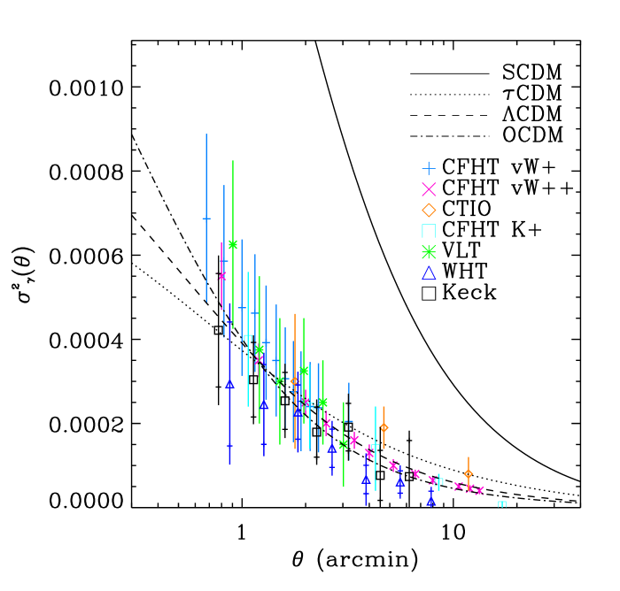
As they travel from a background galaxy to the observer, photons get deflected by mass fluctuations along the line of sight. As a result, the apparent images of background galaxies are subject to a distortion which is characterised by the shear tensor $\gamma_{i}$. The shear component $\gamma_{1}$ ($\gamma_{2}$) describes stretches and compressions along (at $45^{\circ}$ from) the x-axis. The simplest statistics which can be used to characterise the resulting shear patterns on the sky is the the shear variance $\sigma_{\gamma}^{2}(\theta)$ in circular cells of radius $\theta$. The measurements of $\sigma_{\gamma}^{2}(\theta)$ by the different ground-based groups are shown in Figure 5. Recently, cosmic shear has also been detected from space using HST rho99 ; hae01 (not shown on the figure). The agreement between the different groups is impressive given that they used different telescopes and independent data analysis methods. The curves in the figure show the predictions for several CDM models. The measurements are in good agreement with cluster normalised models ($\Lambda$ CDM, OCDM and $\tau$CDM with $\sigma_{8}(\Omega_{m}/0.3)^{0.5}\simeq 1$).

Figure 5: The shear variance $\sigma_{\gamma}^{2}$ as a function of the radius of a circular aperture measured by several groups. The lines represent the predictions of the different CDM models. The ground based observations correspond to that of Wittman et al. (wit00 , CTIO), van Waerbeke et al. (van00 , CFHT vW+), Bacon et al. (bac01 , WHT and Keck), Kaiser, Wilson & Luppino (kai+00 , CFHT K+), Maoli et al. (mao01 , VLT), and van Waerbeke et al. (van01 , CFHT vW++). When applicable, the inner error bars correspond to noise only, while the outer error bars correspond to the total error (noise + cosmic variance). The measurements are all consistent with the cluster normalised CDM models.

The amplitude and scale dependence of the cosmic shear signal depends strongly on the cosmological model. Measurements of the weak lensing power spectrum can thus be used to constrain cosmological parameters, such as $\Omega_{m}$, $\Omega_{\Lambda}$, $\sigma_{8}$, $\Gamma$, etc jai97 ; ber97 ; hu+99 ; van+98 . A precision of order of 10% on these parameters can be achieved with weak lensing surveys of about 10 square degrees. Such cosmic shear surveys can also be combined with CMB anisotropy measurements to break degeneracies present when the CMB alone is considered. This would yield improvements in the precision on cosmological parameters by about one order of magnitude hu+99 .

The shear field is not gaussian, but, instead, has coherent structures on various scales. Bernardeau, van Waerbeke, & Mellier ber97 have shown that the skewness $S_{3}^{\kappa}=\langle\kappa^{3}\rangle/\langle\kappa^{2}\rangle^{2}$ of the convergence field $\kappa$ (which can be derived from the shear field) can be used to break the degeneracy between $\sigma_{8}$ and $\Omega_{m}$, which is present when the shear variance alone is considered. Figure 6 shows the skweness as a function of angular scales expected in several cosmological models.

Figure 6: The solid and dotted lines show respectively the lensing convergence skewness as a function of angular scale for a $\Lambda$CDM (dominated by cosmological constant) model and for a qCDM model (dominated by quintessence or dark energy with equation of state: pressure/density $=-1/2$). Points with error-bars show simulated measurements with the expected statistical error for a $3^{0}\times 3^{0}$ weak-lensing survey with about $30$ galaxies per square arc-minute, where the galaxy median redshift is unity. Note that $S_{3}^{\kappa}$ is largely independent of the details of the mass power spectrum. See huilens for details.

The existing measurements described above are primarily limited by statistics. They will therefore be improved upon by future ground-based instruments, such as Megacam on CFHT bou00 , VISTA tay01 , LSST tys01 , or the novel WFHRI concept kai+00b . From space, the upcoming camera ACS on HST, and, much more ambitiously, the future satellites SNAP per01 and GEST ben01 also offer exciting prospects. Broadly speaking, ground based measurements will cover large areas, while space-based surveys will yield higher resolution maps and reduced systematics thanks to the absence of atmospheric seeing.

These future surveys will provide very accurate measurements of cosmological parameters through the measurement of the weak lensing power spectrum and higher-order statistics. They will also allow us to test some of the foundations of the standard cosmological model. For instance, the measurement of the power spectrum at different redshift slices and of the hierarchy of high-order correlation functions, will yield a direct test of the gravitational instability paradigm. Cosmic shear can also be used to measure the equation of state of the dark energy, and thus complement supernovae measurements in the constraining of quintessence models hut01 ; ben01 ; hu01 . Figure 6 shows how the skewness of the convergence field can be used to distinguish a $\Lambda$CDM model from a qCDM model. Cosmic measurements can also be used to test general relativity itself uza01 .

For these instruments to yield to full promises of cosmic shear, a number of challenges have to be met. First, observationally, systematic effects, such as the PSF anisotropy, CCD non-linearities, etc, must be controlled and corrected for. From the theoretical point of views, calculations of the non-linear power spectrum, of high order statistics and of the associated errors must be improved to meet the precision of future measurements. The observational and theoretical efforts required to overcome these difficulties are very much worth while given the remarkable promisses which cosmic shear offers to cosmology.

VI.2 Lyman-alpha Forest

Another emerging technique is the use of quasar absorption spectra at redshifts $z\sim 2-5$. The main idea is that fluctuations in (Lyman-alpha) absorption (known as the Lyman-alpha forest) can be directly related to fluctuations in the mass density, as illustrated in Fig. 7.

Figure 7: The bottom panel shows the baryon density fluctuation as a function of distance along a line of sight; the next panel up shows the total velocity (peculiar velocity plus Hubble flow) along the same. The top panel shows the corresponding $e^{-\tau}$, where $\tau$ is the optical depth and $e^{-\tau}$ is the probability of transmission, if peculiar velocities are ignored; the panel below shows the same when distortions due to peculiar velocities are taken into account. Note how $e^{-\tau}$, which is proportional to the observed flux of some quasar, provides almost a mirror image of the density profile, modulo peculiar velocities.

Numerical simulations and semi-analytical calculations show that the observed absorption fluctuations and several of their key characteristics can be attributed to mildly non-linear mass fluctuations ($\delta\sim 1$), which arise as a natural consequence of gravitational instability forestpapers . In addition to allowing a measurement of the large scale structure and its growth at redshifts of a few croft , quasar spectra also offer a geometrical method to measure the cosmological constant via the well-known Alcock-Paczynski effect ap . The idea here is also quite simple. Consider a spherical ball placed at redshifts of a few. Its observed shape will be characterized by its redshift-extent and angular-extent. The presence of a cosmological constant turns out to distort the shape in a distinctive way, that cannot be mimicked by for instance spatial curvature: if the cosmological constant (or dark energy component with suitable equation of state to cause acceleration) is significant, the ball will appear squashed in the redshift direction. The abstract “ball” that the forest offers its the two-point correlation function of the absorption fluctuations, measured along sightlines to individual quasars, as well as across sightlines of close quasars apforest . Such a test can be carried out with correlation functions of other objects as well, such as galaxies and quasars galQap . At least one advantage of using the Lyman-alpha forest is that the mapping from mass fluctuation to absorption fluctuation is completely fixed by observations, allowing an estimate of distortions due to peculiar velocities, which must be accounted for in any application of the Alcock-Paczynski test using correlation functions velap .

VI.3 Conclusion

In summary, with the combination of new observational windows such as weak gravitational lensing and the Lyman-alpha forest, and the advent of large galaxy surveys, including the Two-degree-Field Survey and the Sloan Digital Sky Survey, the prospects of using large scale structure to constrain particle physics look brighter than ever.

References

- (1) Freedman, W.L., et al. 2001, ApJ, 553, 47.
- (2) Ajhar, E.A., et al. 2001, 559, 584.
- (3) Parodi, B.R., Saha, A., Sandage, A., & Tammann, G.A. 2000, ApJ, 540, 634.
- (4) Phillips, M.M., et al. 1999, AJ, 118, 1766.
- (5) Garnavich, P.M., et al. 2001, ApJ, in press, astroph/105490.
- (6) Jha, S., et al. 1999, ApJS, 125, 73.
- (7) Mason, B.S., Myers, S.T., & Readhead, A.C.S. 2001, ApJ, 555, 11.
- (8) Williams, L.L.R., & Saha, P. 2000, AJ, 119, 439.
- (9) Perlmutter, S. et al. Astrophys. J. 517, 565 (1999).
- (10) Riess, A.G. et al. Astron. J. 116, 1009 (1998).
- (11) Riess, A.G. et al. Astrophys. J. 560, 49 (2001).
- (12) A. Goobar and S. Perlmutter, Astrophys. J. 450, 14 (1995).
- (13) Bahcall, N. and Fan, X. et al., Astrophys. J. 504, 1 (1998).
- (14) Melchiorri, A. et al., Astrophys. J. 536, 63 (2000).
- (15) Balbi, A. et al., Astrophys. J. 545, L1 (2000)
- (16) Perlmutter, S. et al., Nature, 391, 51 (1998).
- (17) Garnavich, P. et al., Astrophys. J. 509, 74 (1998).
- (18) Weller, J. and Albrecht, A., astro-ph/0106079 (2001).
- (19) B. Ratra and P. J. Peebles, Phys. Rev. D 37, 3406 (1988).
- (20) P. J. Peebles and B. Ratra, Astrophys. J. 325, L17 (1988).
- (21) J. A. Frieman, C. T. Hill, A. Stebbins and I. Waga, Phys. Rev. Lett. 75, 2077 (1995).
- (22) K. Coble, S. Dodelson and J. A. Frieman, Phys. Rev. D 55, 1851 (1997).
- (23) R. R. Caldwell, R. Dave and P. J. Steinhardt, Phys. Rev. Lett. 80, 1582 (1998).
- (24) L. Wang, R. R. Caldwell, J. P. Ostriker and P. J. Steinhardt, Astrophys. J. 530, 17 (2000).
- (25) N. Bahcall, J. P. Ostriker, S. Perlmutter and P. J. Steinhardt, Science 284, 1481 (1999).
- (26) P. deBernardis et al., astro-ph/0105296 (2001).
- (27) I. Maor, R. Brustein and P. J. Steinhardt, Phys. Rev. Lett. 86, 6 (2001) [Erratum-ibid. 87, 049901 (2001)].
- (28) P. M. Garnavich et al., Astrophys. J. 509, 74 (1998).
- (29) S. Perlmutter, M. S. Turner and M. J. White, Phys. Rev. Lett. 83, 670 (1999)
- (30) G. Efstathiou, astro-ph/9904356.
- (31) J. A. Newman and M. Davis, astro-ph/9912366.
- (32) Z. Haiman, J. J. Mohr and G. P. Holder, astro-ph/0002336.
- (33) D. Huterer and M. S. Turner, astro-ph/0012510.
- (34) P. J. Steinhardt, L. Wang and I. Zlatev, Phys. Rev. D 59, 123504 (1999).
- (35) I. Zlatev, L. Wang and P. J. Steinhardt, Phys. Rev. Lett. 82, 896 (1999).
- (36) R. R. Caldwell, astro-ph/9908168.
- (37) C. Armendariz-Picon, V. Mukhanov and P. J. Steinhardt, Phys. Rev. Lett. 85, 4438 (2000).
- (38) C. Armendariz-Picon, V. Mukhanov and P. J. Steinhardt, Phys. Rev. D 63, 103510 (2001).
- (39) V. Sahni and L. Wang, Phys. Rev. D 62, 103517 (2000).
- (40) S. Dodelson, M. Kaplinghat and E. Stewart, Phys. Rev. Lett. 85, 5276 (2000).
- (41) R. R. Caldwell, Braz. J. Phys. 30, 215 (2000); (available at www.dartmouth.edu/ caldwell/research.htm).
- (42) S. M. Carroll, Phys. Rev. Lett. 81, 3067 (1998).
- (43) L. Amendola, Phys. Rev. D 62, 043511 (2000).
- (44) C. Baccigalupi, S. Matarrese and F. Perrotta, Phys. Rev. D 62, 123510 (2000).
- (45) Peebles, P. J. E., 1980, Large Scale Structure of the Universe, Princeton University Press
- (46) Bernardeau, F., Colombi, S., Gaztanaga, E. & Scoccimarro, R. 2001, Large-Scale Structure of the Universe and Cosmological Perturbation Theory, to appear in Physics Reports
- (47) Several textbooks this overall paradigm in depth. They include: Peebles, P. J. E., 1993, Principles of Physical Cosmology, Princeton University Press; Kolb, E. W. & Turner, M. S., 1990, The Early Universe, Addison Wesley; Padmanabhan, T., 1993, Structure Formation in the Universe, Cambridge University Press; Peacock, J. A., 1999, Cosmological Physics, Cambridge; Liddle, A. R. & Lyth, D. H., 2000, Cosmological Inflation and Large Scale Structure, 2000, Cambridge University Press.
- (48) Fry, J. N. 1984, ApJ, 277, L5; Fry, J. N. 1984, ApJ, 279, 499
- (49) Davis, M. & Peebles, P. J. E. 1977, ApJS, 34, 425
- (50) Bernardeau, F. 1994, AAP, 291, 697
- (51) Gaztanaga, E. 1994, MNRAS, 268, 913
- (52) Szapudi, I., Dalton, G. B., Efstathiou, G., & Szalay, A. S. 1995, ApJ, 444, 520; Colombi, S., Szapudi, I., & Szalay, A. S. 1998, MNRAS, 296, 253
- (53) Hui, L. & Gaztañaga, E. 1999, ApJ, 519, 622
- (54) Scoccimarro, R. ;., Feldman, H. A., Fry, J. N., & Frieman, J. A. 2001, ApJ, 546, 652
- (55) Fry, J. N. & Gaztanaga, E. 1993, ApJ, 413, 447.
- (56) Mo, H. J. & White, S. D. M. 1996, MNRAS, 282, 347
- (57) Pen, U. 1998, ApJ, 504, 601; Dekel, A. & Lahav, O. 1999, ApJ, 520, 24
- (58) Fry, J. N. 1994, Physical Review Letters, 73, 215
- (59) Giavalisco, M., Steidel, C. C., Adelberger, K. L., Dickinson, M. E., Pettini, M., & Kellogg, M. 1998, ApJ, 503, 543; Adelberger, K. L., Steidel, C. C., Giavalisco, M., Dickinson, M., Pettini, M., & Kellogg, M. 1998, ApJ, 505, 18
- (60) Fry, J. N. 1996, ApJ, 461, L65
- (61) Tegmark, M. & Peebles, P. J. E. 1998, ApJ, 500, L79
- (62) See for an excellent review: Bertschinger, E. 1995, Cosmological Dynamics, Les Houches 1993 Lectures, astro-ph 9503125
- (63) Bertschinger, E. & Dekel, A. 1989, ApJ, 336, L5
- (64) Dekel, A., Bertschinger, E., Yahil, A., Strauss, M. A., Davis, M., & Huchra, J. P. 1993, ApJ, 412, 1
- (65) Kaiser, N. 1987, MNRAS, 227, 1
- (66) Fisher, K. B., Davis, M., Strauss, M. A., Yahil, A., & Huchra, J. P. 1994, MNRAS, 267, 927; Cole, S., Fisher, K. B., & Weinberg, D. H. 1995, MNRAS, 275, 515
- (67) See for an excellent review: Hamilton, A. J. S. 1998, ASSL Vol. 231: The Evolving Universe, 185
- (68) Zehavi, I. & Dekel, A. 1999, Nature (London), 401, 252; Willick, J. A. & Strauss, M. A. 1998, ApJ, 507, 64
- (69) Peacock, J. A. et al. 2001, Nature, 410, 169
- (70) Riess, A. G., Davis, M., Baker, J., & Kirshner, R. P. 1997, ApJ, 488, L1
- (71) e.g. Tonry, J. L., Blakeslee, J. P., Ajhar, E. A., & Dressler, A. 2000, ApJ, 530, 625;
- (72) de Bernardis, P. et al. 2000, Nature (London), 404, 955; Netterfield et al. 2001, submitted to ApJ, astro-ph 0104460; Pryke et al. 2001, submitted to ApJ, astro-ph 0104490; Lee, A. T. et al. 2001, astro-ph 0104459 Wang, Tegmark & Zaldarriaga 2001, astro-ph 0105091
- (73) Riess, A. G. et al. 1998, AJ, 116, 1009; Perlmutter, S. et al. 1999, ApJ, 517, 565
- (74) For a recent impressive test, see consistency among independent measurements of the baryon density: Burles, S. and Tytler, D. 1998, ApJ, 507, 732-744; Burles, S., Nollett, K. M., & Turner, M. S. 2001, ApJ, 552, L1; and ref. in boompapers .
- (75) White, S. D. M., Efstathiou, G., & Frenk, C. S. 1993, MNRAS, 262, 1023; Bahcall, N. A. & Fan, X. 1998, ApJ, 504, 1; Viana, P. T. P. & Liddle, A. R. 1999, MNRAS, 303, 535
- (76) Robinson, J., Gawiser, E., & Silk, J. 2000, ApJ, 532, 1
- (77) White, S. D. M. & Rees, M. J. 1978, MNRAS, 183, 341
- (78) For an excellent review, see: White, S. D. M. 1994, Formation and Evolution of Galaxies: Les Houches Lectures, astro-ph 9410043
- (79) See review by Bertschinger, E. 1998, ARA&A, 36, 599
- (80) Bond, J. R., Cole, S., Efstathiou, G., & Kaiser, N. 1991, ApJ, 379, 440; Lacey, C. & Cole, S. 1993, MNRAS, 262, 627; Sheth, R. K. & Lemson, G. 1999, MNRAS, 305, 946
- (81) Peacock, J. A. & Smith, R. E. 2000, MNRAS, 318, 1144; Seljak, U. ; 2000, MNRAS, 318, 203; Ma, C. & Fry, J. N. 2000, ApJ, 531, L87; Sheth, R. K., Hui, L., Diaferio, A., & Scoccimarro, R. ;. 2001, MNRAS, 325, 1288; Scoccimarro, R. ;., Sheth, R. K., Hui, L., & Jain, B. 2001, ApJ, 546, 20; Cooray, A. 2001, astro-ph 0105440; Berlind, A. A., & Weinberg, D. H. 2001, submitted to ApJ, astro-ph 0109001
- (82) Peebles, P. J. E. 2001, ApJ, 557, 495; Ellis, R. S., Abraham, R. G. & Dickinson, M. 2000, ApJ in press, astro-ph 0010401
- (83) Hui, L. 1999, ApJ, 519, L9
- (84) McGill, C. 1990b, MNRAS, 242, 544; Bi, H. G., Boerner, G. and Chu, Y. 1992, A & A; Cen, R., Miralda-Escude, J., Ostriker, J. P. and Rauch, M. 1994, ApJ Lett, 437, L9-L12; Zhang, Y., Anninos, P. and Norman, M. L. 1995, ApJ Lett, 453, L57-59; Reisenegger, A. and Miralda-Escude, J. 1995, ApJ, 449, 476-490; Petitjean, P., Mueket, J. P., & Kates, R. E. 1995, AAP, 295, L9; Hernquist, L., Katz, N., Weinberg, D. H., & Jordi, M. 1996, ApJ, 457, L51; Miralda-Escude, J., Cen, R., Ostriker, J. P. and Rauch, M. 1996, ApJ, 471, 582; Bond J.R., Wadsley J.W., 1997, Proc. 12th Kingston Conf.; Bi, H. and Davidsen, A. F. 1997, ApJ 479, 523-527; Hui, L., Gnedin, N. Y. and Zhang, Y. 1997, ApJ, 486, 599-610; Hui, L. and Gnedin, N. Y. 1997, MNRAS, 292, 27-35; Zhang, Y., Anninos, P., Norman, M. L. and Meiksin, A. 1997, ApJ, 485, 496-523; Haehnelt, M. G. & Steinmetz, M. 1998, MNRAS, 298, L21; Theuns, T., Leonard, A., Efstathiou, G., Pearce, F. R., & Thomas, P. A. 1998, MNRAS, 301, 478.
- (85) Croft, R. A. C., Weinberg, D. H., Katz, N. and Hernquist, L. 1998, ApJ, 495, 44-55; Croft, R. A. C., Weinberg, D. H., Pettini, M., Hernquist, L. and Katz, N. 1999, ApJ, 520, 1-23; McDonald, P., Miralda-Escud/’e, J., Rauch, M., Sargent, W. L. W., Barlow, T. A., Cen, R., & Ostriker, J. P., 1999, ApJ, in press, astro-ph 9911196; Zaldarriaga, M., Hui, L. & Tegmark, M. 2000, ApJ, in press, astro-ph 0011559
- (86) Alcock, C. and Paczynski, B. 1979, Nature, 281, 358-361.
- (87) Hui, L., Stebbins, A. and Burles, S. 1999, ApJ Lett, 511, L5-L8; McDonald, P. and Miralda-Escudé, J. 1999, ApJ, 518, 24-31
- (88) Matsubara, T. & Suto, Y. 1996, ApJ, 470, L1; Popowski, P. A., Weinberg, D. H., Ryden, B. S., & Osmer, P. S. 1998, ApJ, 498, 11; de Laix, A. A. & Starkman, G. 1998, ApJ, 501, 427; Hoyle, F., Outram, P. J., Shanks, T., Boyle, B. J., Croom, S. M. & Smith, R. J. astro-ph 0107348
- (89) Hui, L. 1999, ApJ, 516, 519; McDonald, P. 2001, submitted to ApJ, astro-ph 0108064
- (90) Guth, A. H. Phys. Rev. D 1981, 23, 347; Linde, A. D. Phys. Lett. 1982, B108 389; Albrecht, A. & Steinhardt, P. J., 1982, Phys. Rev. Lett 48, 1220.
- (91) Hu, W., Fukugita, M., Zaldarriaga, M., & Tegmark, M. 2001, ApJ, 549, 669
- (92) See e.g. Lidsey, J. E., Liddle, A. R., Kolb, E. W., Copeland, E. J. Barreiro, T., and Abney, M. 1997, Rev. Mod. Phys. 69, 373 and references therein.
- (93) Nusser, A., Dekel, A., & Yahil, A. 1995, ApJ, 449, 439; Scoccimarro, R. ;., Feldman, H. A., Fry, J. N., & Frieman, J. A. 2001, ApJ, 546, 652; Verde, L., Jimenez, R., Kamionkowski, M., & Matarrese, S. 2001, MNRAS, 325, 412; Ferreira, P. G., Gorski, K. M. & Magueijo, J. 1999, astro-ph 9904073; Wu, J. H. P., et al. astro-ph 0104248; Santos, M. G. et al. 2001, astro-ph 0107588
- (94) e.g. Allen, B., Caldwell, R. R., Dodelson, S., Knox, L., Shellard, E. P. S., & Stebbins, A. 1997, PRL, 79, 2624; Pen, U., Seljak, U., & Turok, N. 1997, PRL, 79, 1611
- (95) Bucher, M., Moodley, K. & Turok, N. 2000, astro-ph 0012141
- (96) Shiu, S. & Tye, S. H. H. hep-th/0106274; but see also Huey, G. & Lidsey, J. E. 2001, Phys. Lett. B514, 217; Liddle, A. R. & Taylor, A. N. 2001, astro-ph 0109412
- (97) Martin, J. & Brandenberger, R. H. Phys. Rev. 2001, D63, 123501; Brandenberger, R. H. & Martin, J. Mod. Phys. Lett. 2001, A16, 999; Niemeyer, J. C. Phys. Rev. 2001, D63, 123502; Kempf, A. astro-ph/0009209; Tanaka, T. astro-ph/0012431, Starobinsky, A. A. Pisma Zh. Eksp. Teor. Fiz. 2001, 73, 415; Easther, R., Greene, B., Kinney, W. H. & Shiu, G. hep-th/0104102; Hui, L. & Kinney, W. H., 2001, astro-ph 0109107
- (98) Hu, W., Eisenstein, D. J. & Tegmark, M. 1998, PRL, 80, 5255; Croft, R. A. C., Hu, W. & Dave, R. 1999, PRL, 83, 1092
- (99) Flores, R. & Primack, J. 1994, ApJ, 427, L1; Moore, B. 1994, Nature, 370, 629; Spergel, D. N. & Steinhardt, P. J. 2000, PRL, 84, 3760
- (100) Navarro, J. R., Eke, V. R. & Frenk, C. S., 1996, MNRAS, 283, L72; Gnedin, O. Y. & Zhao, H. S. 2001, astro-ph 0108108; Binney, J., Gerhard, O., & Silk, J. 2000, astro-ph 0003199
- (101) Bartelmann, M., & Schneider, P. 1999, submitted to Physics Reports, preprint astro-ph/9912508
- (102) Mellier, Y., et al., 2001, to appear in ESO proceedings, Deep Fields, Garching Oct 2000, preprint astro-ph/0101130
- (103) Bacon, D.J., Refregier, A., & Ellis, R. 2000, MNRAS, 318, 625
- (104) Wittman, D.M., Tyson, J., Kirkman, D., Dell’Antonio, I., Bernstein, G., 2001, Nature, 405, 143
- (105) van Waerbeke, L., et al. 2000, A&A, 358, 30
- (106) van Waerbeke, L., et al. 2001, A&A, 374, 757
- (107) Kaiser, N., Wilson, G., & Luppino, G.A., 2000, submitted to ApJL, preprint astro-ph/0003338
- (108) Rhodes, J., Refregier, A., & Groth, E., 2001, ApJ, 552L, 85
- (109) Maoli, R., et al., 2001, A&A, 368, 766
- (110) Heammerle et al. 2001, submitted to A&A, preprint astro-ph/0110210
- (111) Bacon, D.J., Massey, R., Refregier, A. & Ellis, R.S., 2001, in preparation
- (112) Jain, B. & Seljak, U. 1997 ApJ 484, 560.
- (113) Bernardeau, F., van Waerbeke, L., & Mellier, Y., 1997, A&A, 322, 1
- (114) Kaiser, N. 1998 ApJ, 498, 26.
- (115) Hu, W. & Tegmark, M. 1999, ApJ, 514L, 65
- (116) van Waerbeke, L., Bernardeau, F., Mellier, Y., 1999, A&A, 342, 15
- (117) Boulade, O. et al., 2000, Procs. of SPIE’s Astronomical Telescopes and Instrumentation 2000, Munich, 2000; Megacam home page http://www-dapnia.cea.fr/Phys/Sap/Activites/Projets/Megacam/page.shtml
- (118) Taylor, A., et al. 2001, in preparation; see also VISTA home page http://www.vista.ac.uk
- (119) Tyson, J.A., 2001, LSST home page http://www.lssto.org/lssto/index.htm
- (120) Kaiser, N., Tonry, J.L., Luppino, G.A., 2000, PASP,112,768
- (121) Perlmutter et al. 2001, SNAP home page http://snap.lbl.gov
- (122) Bennet, D.P., & Rhie, S.H., 2000, submitted to ApJ, preprint astro-ph/0011466; GEST home page http://bustard.phys.nd.edu/GEST
- (123) Huterer, D., 2001, preprint astro-ph/0106399
- (124) Hu, W., 2001, submitted to PRD, preprint astro-ph/010890
- (125) Uzan, J.-P., & Bernardeau, F., 2001, PRD, 64, 083004
- (126) Resource Book on Dark Energy, ed. Eric Linder http://supernova.lbl.gov/ẽvlinder/sci.html