Chandra temperature and metallicity maps of the Perseus cluster core

Abstract

We present temperature and metallicity maps of the Perseus cluster core obtained with the Chandra X-ray Observatory. We find an overall temperature rise from $\sim 3.0$ keV in the core to $\sim 5.5$ keV at 120 kpc and a metallicity profile that rises slowly from $\sim 0.5$ solar to $\sim 0.6$ solar inside 60 kpc, but drops to $\sim 0.4$ solar at 120 kpc. Spatially resolved spectroscopy in small cells shows that the temperature distribution in the Perseus cluster is not symmetrical. There is a wealth of structure in the temperature map on scales of $\sim 10$ arcsec (5.2 kpc) showing swirliness and a temperature rise that coincides with a sudden surface brightness drop in the X-ray image. We obtain a metallicity map of the Perseus cluster core and find that the spectra extracted from the two central X-ray holes as well as the western X-ray hole are best-fit by gas with higher temperature and higher metallicity than is found in the surroundings of the holes. A spectral deprojection analysis suggests, however, that this is due to a projection effect; for the northern X-ray hole we find tight limits on the presence of an isothermal component in the X-ray hole, ruling out volume-filling X-ray gas with temperatures below 11 keV at 3$\sigma$.

1 Introduction

The Perseus cluster, Abell 426, at a redshift of $z=0.0183$ or distance about 100 Mpc is the the nearest high luminosity cluster with a high central surface brightness (e.g., Fabian et al., 1981; Allen et al., 2001; Fabian, 1994). This makes it the brightest cluster in the X-ray sky.

The first Chandra subarcsecond-resolution X-ray images of the cluster core around the central dominant galaxy NGC 1275 were presented by Fabian et al. (2000, F00). Using X-ray colours F00 showed that the temperature of the gas decreases from about 6.5 keV to 3 keV inward to the central galaxy NGC 1275, which is surrounded by a spectacular low-ionization, emission line nebula (Lynds, 1970, see also Conselice, Gallagher, & Wyse 2001).

The nucleus powers the radio source 3C84 (Pedlar et al 1990) which has structures on various scales. The 0.5 arcmin-sized radio lobes coincide with holes in the soft X-ray emission (Böhringer et al. 1993; McNamara et al. 1996; F00). Chandra has revealed that the holes are not due to absorption and have X-ray bright rims, which are cooler than the surrounding gas (F00). It was found that the rims are not distinguishable as sharp features on a 3–7 keV image and are therefore not shock features, contrary to the early prediction of Heinz, Reynolds & Begelman (1998), and are not expanding supersonically. The simplest interpretation of the low surface brightness is that they are devoid of X-ray gas and have pressure support from cosmic rays and magnetic fields. However they may contain some hotter gas at the virial temperature, or even above, of the cluster with the radio plasma having a low filling factor. In this scenario the rims consist of cooler gas which has been swept aside. The two outer holes, one of which was previously known, were identified with recently-found spurs of low-frequency radio emission by Blundell et al. (2000).

The core of the Perseus cluster offers the rare opportunity to study the radio source/intracluster gas interaction on arcsecond scales. In the present study we have carried out a spectral analysis of the Chandra images which provides us detailed information about the cluster physics. In Sect. 2 we describe the observations including the full 29.0 ks Chandra image of the Perseus cluster core. In Sect. 3 we describe our method of spectral analysis and show temperature and metallicity profiles, as well as maps. In Sect. 4 we carry out a spectral deprojection analysis of the cluster and search for the presence of X-ray gas in the northern X-ray hole. In Sect. 5 we conclude with a summary and a discussion.

We use $H_{0}=50\hbox{$\hbox{${\rm\thinspace km}{\rm\thinspace s}^{-1}\,$}{\rm\thinspace Mpc}^{-1}$}$ and $q_{0}=\frac{1}{2}$ throughout. Unless otherwise stated, quoted error bars are 1 $\sigma$ (68.3% confidence).

2 Observations

Chandra observed the Perseus cluster on 1999 September 20, 1999 November 28 and 2000 January 31 for 5.3 ks, 9 ks and 24.7 ks, respectively. The early observation was carried out with the ACIS-I detector. The energy resolution of this observation has been seriously affected by the radiation damage suffered by the front-illuminated ACIS chips, so that we only use it to produce images. The two later observations were carried out with the ACIS-S detector. The target was centred very close to the middle of the back-illuminated ACIS chip S3 (ACIS-S3). The detector temperature during these observations was -110 C. Inspection of the light curves of the observations showed that the later, longer, observation had been affected by flares, so that we had to clean the light curve. This reduced the exposure time usable for spectroscopic analysis to 14.9 ks.

In Fig. 1 the combined 29.0 ks image of all three Chandra exposures of the Perseus cluster core is shown. The image was constructed by concatenating the three event files using the combine_obsid script available on the Chandra X-ray Observatory Centre (CXC) web pages (www.cxc.edu).

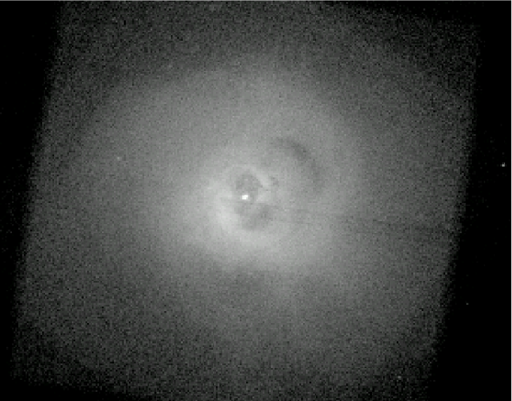
Figure 1: Combined 29.0 ks Chandra image of the Perseus cluster core in the 0.5 to 7 keV band. The image size is 10.1 arcmin $\times$ 7.9 arcmin (312.5 kpc $\times$ 244.4 kpc). The linear boundaries visible at the edges of the frame are due to the three different orientations of the detector in the three added exposures.

The image was binned into (1.97 arcsec)² pixels. The well-known features of the inner X-ray holes and the outer X-ray hole (north-west) can be seen. In this stacked image a streak of emission can be seen running through the southern hole (see also Fabian et al. 2002, hereafter F02). This feature was not obvious in the image studied by F00 due to the dead column feature that runs straight across it in the January 2000 image. The southern outer X-ray hole first discussed by F00 and another similar cavity immediately to the west of it are also visible.

Between the western outer hole and the southern outer hole a curved, elongated feature is apparent with a smaller count rate than in the surrounding area. It appears to be a structure that connects the two outer holes. It is reminiscent of the radio structure apparently connecting the two outer radio lobes of the central radio source 3C 338 in Abell 2199 (Giovannini et al., 1998).

The appearance of swirliness (F00, see also Churazov et al. 2000) in the outer regions of the image is created by a distinct surface brightness drop that broadly coincides with a rise in the X-ray temperature (with increasing radius), as we will show in the next section.

3 Spectral analysis

3.1 Calibration

We extract spectra from regions of the Chandra data set using the CIAO software package distributed by the CXC. We only work with photons detected in the ACIS-S3 chip, which is also known as ACIS chip 7. We also restrict ourselves to the 0.5-7.0 keV band in order to be certain of a reliable energy calibration. Response matrix files (RMF) and ancillary response files (ARF) were produced using the calcrmf and calcarf programs by Alexey Vikhlinin available from the CXC web pages.

Using the task grppha from the FTOOLS software package provided by the NASA High Energy Astrophysics Science Archive Research Center, the extracted spectra are grouped so that we have at least 20 counts in a bin corresponding to a certain range of energy channels. This allows us to use Poisson error bars for spectral fitting.

We have have generated background spectra using Markevitch’s method and program that is also available from the CXC web site. We extract the background data from the same regions on the chip as the spectra extracted from the data sets. In the case of the Perseus cluster core the background in the ACIS-S3 chip in the 0.5-7.0 keV band ($<\,1$ cts s^-1) is much smaller than the signal from the cluster ($83.4$ cts s^-1).

When fitting extracted spectra, we fit the November and the January data set in parallel with the same spectral model, allowing only for a different normalization of the two spectra. The different normalizations are necessary because the exposures are affected by the ACIS-S3 missing column feature in two different orientations. The feature is due to 5 contiguous partially dead columns in the centre of the chip that cause missing counts in an elongated region several arcmin long and approximately 17  arcsec wide (due to the spacecraft dither). This procedure affected only regions covering the dead columns, in other regions the normalizations were consistent with each other.

3.2 Selection of regions

In order to map the spectral properties of the cluster we divide the cluster into cells with a constant number of cluster emission counts. Since the background is not important for Perseus (Sect. 3.1) this is very similar to having an equal number of counts in each cell.

We determine the cell shapes by iteratively dividing annular segments with inner and outer radii $r_{1}$, and r₂ and bounding azimuthal angles $\alpha_{1}$,$\alpha_{2}$ into regions with equal number of counts (corrected for the background contribution as determined from Markevitch’s background files). Beginning with a full circle with radius $r$ ($r_{1}=0$, $r_{2}=r$, $\alpha_{1}=0$, $\alpha_{2}=2\,\pi$) the iterations are either exclusively performed on the radius, yielding a sequence of annuli, or interchangingly on radius and azimuth, yielding a more complex web of cells.

We carry out the analysis on three scales: (1) Simple annuli with $\sim\,$35000 counts each, (2) cells with $\sim\,$18000 counts and (3) cells with $\sim 500$ counts each. The cell divisions were determined using the 14.9 ks exposure taken on 1999 November 28. The mentioned count values in this and the following sections refer to this exposure.

3.3 Annular spectra

We begin the spectral analysis by studying azimuthally averaged spectra from annuli with a large ($\sim\,$35000) number of counts. This will give an overview of the radial variation of the ambient X-ray gas temperature in Perseus.

We use XSPEC (Arnaud, 1996) to fit the X-ray spectra. Errors are determined with the XSPEC tasks error and steppar. We model the X-ray emission from the intracluster gas using the APEC plasma emission code (version 1.10). It is available on the web at hea-www.harvard.edu/APEC and is also included in the latest XSPEC versions. We use this newer code instead of the traditional MEKAL plasma code (Kaastra & Mewe, 1993; Liedahl et al., 1995) because it provides a significant improvement of the spectral fits. For example, when fitting a spectrum extracted from an annulus with inner radius 23  arcsec and outer radius 32  arcsec around the nucleus (542 degrees of freedom) we obtain a $\chi^{2}=625.7$ for the APEC model instead of $\chi^{2}=662.0$ for MEKAL. The change in best-fit parameters, however, is small; the best-fit absorption and temperature are identical for both plasma codes. The metallicity changes slighly, in this particular case from 0.42$\pm 0.03$ solar for MEKAL to 0.46$\pm 0.03$ solar for APEC. A large part of the improvement is due to a better representation of the blue wing of the Fe L complex.

In order to model the emission from a single temperature we fit the spectra with the following model:

$${\rm MODEL}_{1}={\rm PHABS}\,(N_{\rm H})\times{\rm APEC}\,(T,Z,K).$$ (1)

PHABS is the photoelectric absorption model by Balucinska-Church & McCammon (1992). The free parameters equivalent hydrogen column density $N_{\rm H}$, temperature $T$, average metallicity $Z$ (relative to the solar values according to Anders & Grevesse 1989) and spectral normalization $K$ are given in brackets. In Figs. 2, 3 and 4 the results of the spectral fits for the temperature, the metallicity and for the required photoelectric absorption are shown. The fits have been done both with (dotted error bars) and without (solid error bars) fixing the photoelectric absorption. Except for the innermost annulus, the absorption is consistent with being constant (Fig. 4). For the fits with fixed absorption we fixed it at the median of all fitted equivalent hydrogen column densities $N_{\rm H}=0.143\times 10^{22}\hbox{${\rm\thinspace cm}^{-2}\,$}$ because the Galactic value (Dickey & Lockman, 1990) value from H_I studies ($0.149\times 10^{21}\hbox{${\rm\thinspace cm}^{-2}\,$}$) appears to be slightly too high (see Fig. 4). In Tab. 1 we list the details of the fits with free absorption. It can be seen from Figs. 2 and 3 that the best-fit values are very similar for models with or without fixed absorption.

The temperature profile (Fig. 2) reveals a rapid temperature decline from more than 5 keV to about 3 keV in the rims around the inner X-ray holes. Due to the large number of counts, the error bars are very small. There is a sudden jump in the temperature at a radius of 80 kpc, which coincides with the sudden brightness drop seen to the north of the cluster centre (Fig. 1).

Note also that the temperature rises again in the core. In this innermost ring, the nucleus and the inner 2.5 kpc (4.8  arcsec) around it have been cut out. It can be seen from Tab. 1 that the spectral fit in this ring is not as good as the fits in most of the other rings. This region encompasses most of the northern and about half of the southern X-ray hole. It shows signs of excess absorption (Fig. 4) due to the infalling high-velocity system (Unger et al., 1990; de Young et al., 1973; Briggs et al., 1982) that was found in absorption by Chandra (F00). A two-temperature model improves the fit and is favoured by an F-test. The two-temperature fit yields a 4.6 keV gas phase and a 1.9 keV gas phase, where the normalization of the high-temperature phase is twice of the low-temperature phase. It only improves the reduced ${\chi_{\nu}}^{2}$ to 1.34, however, so that this can also not be viewed as an entirely acceptable fit. In general we find that two-temperature fits do not provide a better description of the annular spectra. Overall there is no convincing evidence for multiphase gas in the Chandra spectra of the Perseus cluster.

In the metallicity profile (Fig. 3) a gradient from $Z\sim 0.6$ solar at a radius of 60 kpc to $Z\sim 0.4$ solar at a radius of 120 kpc is seen. There may be a peak of the metallicity profile at $\sim 50-60$ kpc, but the metallicities drop only slightly inwards from 60 kpc towards a central metallicity of $Z\sim 0.5$ solar. Due to the large number of counts in the annuli, the relative errors are normally less than 10 per cent so that the trend between 60  and 120 kpc is detected with high significance.

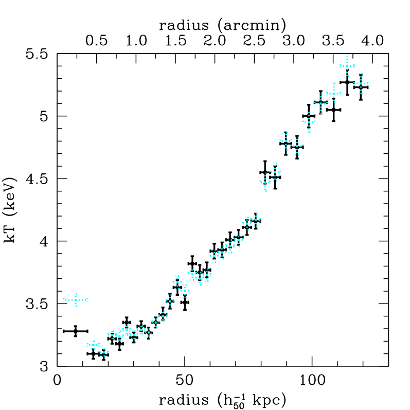
Figure 2: Temperatures from single temperature fits to annular spectra between 2.5 and 121.8 kpc (see also Figs. 3 and 4). The temperatures with solid error bars have been determined without fixing the galactic absorption (see Fig. 4). For the dotted error bars the absorption was fixed to the median of the fitted absorption values, N_H=0.143$\times 10^{22}\hbox{${\rm\thinspace cm}^{-2}\,$}$. Note the jump in the temperature profile at a radius of 80 kpc.

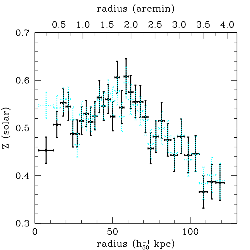
pwd

Figure 3: Metallicity profile from single temperature fits to annular spectra between 2.5 and 121.8 kpc (see also Figs. 2 and 4). The metallicities with solid error bars have been determined without fixing the galactic absorption (Fig. 4). For the dotted error bars the absorption was fixed to the median of the fitted absorption values, N_H=0.143$\times 10^{22}\hbox{${\rm\thinspace cm}^{-2}\,$}$.

Figure 4: Column densities from single temperature fits to annular spectra between 2.5 and 121.8 kpc without fixing the absorbing column density (see also Figs. 2 and 3). The dashed line indicates the median of N_H=0.143$\times 10^{22}\hbox{${\rm\thinspace cm}^{-2}\,$}$.

Table 1: Single temperature fits to azimuthally averaged spectra. The listed parameters are inner and outer radius ($r_{1}$, $r_{2}$), temperature (column 3), metallicity (column 4) and equivalent absorbing hydrogen column density (column 5). Describing the goodness of fit we also list the $\chi^{2}$ value, the number of degrees of freedom (DOF) and the reduced ${\chi_{\nu}}^{2}$ (columns 6 to 8).

$r_{1}$ (kpc)	$r_{2}$ (kpc)	kT (keV)	$Z$ (solar)	$N_{\rm H}$	$\chi^{2}$	DOF	${\chi_{\nu}}^{2}$
				(1021 cm-2)
2.5	11.9	3.28$\pm{0.04}$	0.45$\pm{0.03}$	1.62$\pm{0.03}$	746.7	541	1.38
11.9	16.5	3.10$\pm{0.04}$	0.51$\pm{0.03}$	1.50$\pm{0.03}$	593.0	542	1.09
16.5	20.0	3.09$\pm{0.04}$	0.55$\pm{0.03}$	1.44$\pm{0.03}$	597.6	531	1.13
20.0	23.1	3.22$\pm{0.04}$	0.55$\pm{0.03}$	1.46$\pm{0.03}$	607.3	533	1.14
23.1	25.9	3.18${}^{+0.04}_{-0.05}$	0.49$\pm{0.03}$	1.49$\pm{0.03}$	541.7	532	1.02
25.9	28.7	3.35$\pm{0.04}$	0.49$\pm{0.03}$	1.38$\pm{0.03}$	679.1	549	1.24
28.7	31.5	3.23$\pm{0.04}$	0.52$\pm{0.03}$	1.45$\pm{0.03}$	636.9	540	1.18
31.5	34.5	3.32$\pm{0.04}$	0.53$\pm{0.03}$	1.40$\pm{0.03}$	714.8	565	1.27
34.5	37.3	3.27${}^{+0.04}_{-0.05}$	0.51$\pm{0.03}$	1.44$\pm{0.03}$	724.3	539	1.34
37.3	40.1	3.35$\pm{0.04}$	0.53$\pm{0.03}$	1.43$\pm{0.03}$	620.3	545	1.14
40.1	42.9	3.41${}^{+0.06}_{-0.04}$	0.56${}^{+0.04}_{-0.03}$	1.42$\pm{0.03}$	649.6	550	1.18
42.9	45.7	3.52$\pm{0.06}$	0.55$\pm{0.03}$	1.43$\pm{0.03}$	587.8	544	1.08
45.7	48.7	3.63$\pm{0.06}$	0.56$\pm{0.03}$	1.46$\pm{0.03}$	635.0	565	1.12
48.7	51.5	3.51$\pm{0.06}$	0.52$\pm{0.03}$	1.50$\pm{0.03}$	588.0	548	1.07
51.5	54.5	3.82$\pm{0.06}$	0.61$\pm{0.03}$	1.37$\pm{0.03}$	678.2	573	1.18
54.5	57.3	3.75$\pm{0.06}$	0.54${}^{+0.04}_{-0.03}$	1.39$\pm{0.03}$	622.1	552	1.13
57.3	60.1	3.77$\pm{0.06}$	0.61$\pm{0.04}$	1.41$\pm{0.03}$	592.3	550	1.08
60.1	63.2	3.92$\pm{0.06}$	0.57${}^{+0.04}_{-0.03}$	1.40$\pm{0.03}$	617.9	574	1.08
63.2	66.2	3.93$\pm{0.06}$	0.56${}^{+0.04}_{-0.03}$	1.42$\pm{0.03}$	740.8	570	1.30
66.2	69.5	4.01$\pm{0.06}$	0.56$\pm{0.03}$	1.39$\pm{0.03}$	763.0	579	1.32
69.5	72.8	4.03$\pm{0.06}$	0.52$\pm{0.03}$	1.41$\pm{0.03}$	634.5	571	1.11
72.8	76.1	4.11$\pm{0.06}$	0.46$\pm{0.03}$	1.45$\pm{0.03}$	534.2	569	0.94
76.1	79.7	4.16$\pm{0.06}$	0.48$\pm{0.03}$	1.43$\pm{0.03}$	724.3	577	1.26
79.7	83.5	4.55$\pm{0.09}$	0.52$\pm{0.04}$	1.39$\pm{0.03}$	692.1	589	1.18
83.5	87.5	4.51$\pm{0.09}$	0.47${}^{+0.04}_{-0.03}$	1.45$\pm{0.03}$	651.1	596	1.09
87.5	91.8	4.78$\pm{0.09}$	0.44${}^{+0.04}_{-0.03}$	1.44$\pm{0.03}$	666.4	598	1.11
91.8	96.4	4.75$\pm{0.09}$	0.48$\pm{0.04}$	1.43$\pm{0.03}$	688.0	597	1.15
96.4	101.0	5.00$\pm{0.09}$	0.44$\pm{0.04}$	1.40$\pm{0.03}$	698.2	592	1.18
101.0	105.8	5.11$\pm{0.09}$	0.45$\pm{0.04}$	1.42$\pm{0.03}$	659.4	603	1.09
105.8	111.1	5.05$\pm{0.09}$	0.37$\pm{0.03}$	1.49$\pm{0.03}$	686.9	612	1.12
111.1	116.4	5.27$\pm{0.10}$	0.39$\pm{0.04}$	1.49$\pm{0.03}$	663.2	608	1.09
116.4	121.8	5.23$\pm{0.10}$	0.39$\pm{0.04}$	1.44$\pm{0.03}$	664.3	592	1.12

3.4 Spectra in large cells

Following on to the azimuthally averaged spectra we next present the results from cells with $\sim 18000$ counts. In the left panel of Fig. 5 the definition of the cells and the intensity map of the cluster with this resolution are shown. The contours of the Chandra image are overlaid on top. The middle and right panels are maps of the temperature and the average metallicity determined using the single temperature model in eq. (1) with free Galactic absorption. The statistical uncertainty of the temperatures is less than 0.1 keV, the uncertainty of the metallicities is less than 10 per cent.

It was shown by F00 using X-ray colours that the temperature distribution in the region is not circularly symmetric. The middle panel in Fig. 5 illustrates the overall temperature distribution obtained with the APEC plasma model fits in a region of $\sim 125$ kpc radius around the nucleus. The large asymmetric region in the centre at a temperature of 3 to 4 keV is surrounded by hotter gas with temperatures up to 6 keV. The cool region is extended towards the north and the west, whereas in the south-east hotter gas is found at smaller radii. A comparison with the intensity contours in the left panel shows that the outer intensity contour has a similar shape to the isotherms at that radius; the inward (towards smaller radii) bend of the outer intensity contour to the south east of the cluster centre coincides with a high-temperature region. The spectra extracted from the regions corresponding to the inner X-ray holes and the outer hole (see the lighter cell the left panel of Fig. 5) in the west are best-fit by gas at a higher temperature than is found in their immediate surroundings. The same may be true for the less obvious southern X-ray hole discovered by F00 (see Fig. 1), but here the distinction from the hotter gas that intrudes from the south-east is not clear.

In the metallicity map (Fig. 5, right panel) small variations of the metallicities are apparent between cells at similar radii. A high-metallicity ring ($\sim 0.6$ solar) around the cluster centre is prominently seen at a radius of $\sim 60\,$kpc where the peak in the azimuthally averaged metallicity distribution in Fig. 3 was found. In addition to the higher temperature, the spectra extracted from the inner X-ray holes and the western hole are also best-fit by gas with a higher metallicity than is found in their immediate surroundings.

We note that a comparison with the galaxy distribution in an optical Digitial Sky Survey image of this region does not yield any obvious correlation. Due to the relatively coarse scale of the metallicity map, and due to projection effects, however, the question of correlations between the metal distribution and the galaxy distribution cannot be answered by this data set. Nevertheless, it is exciting that the Chandra X-ray observations begin to approach answering such questions.

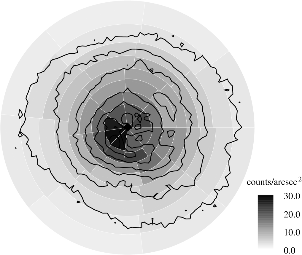
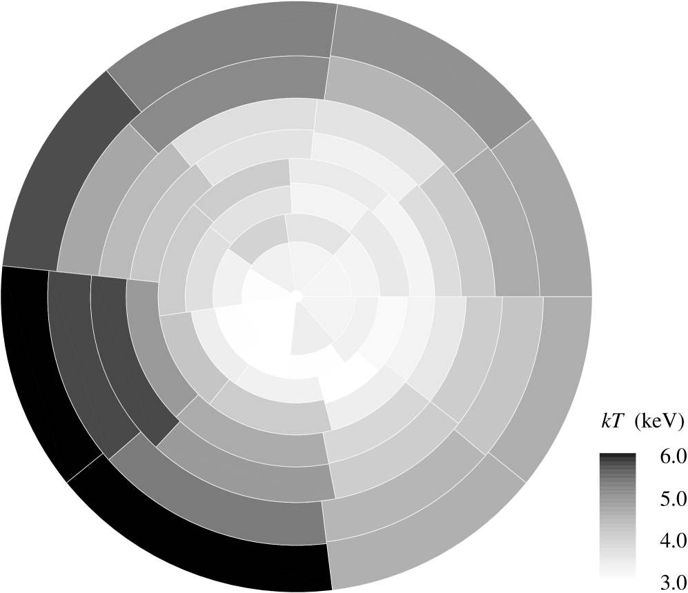
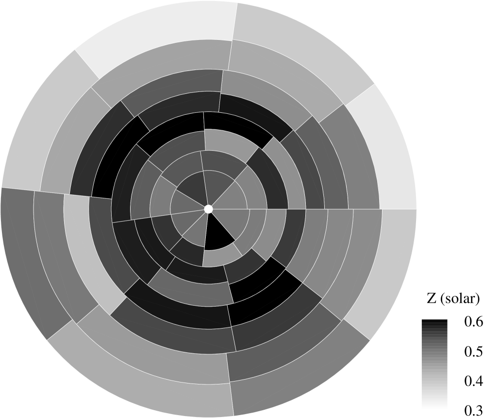
Figure 5: Intensity (left), temperature (middle) and metallicity (right) maps of the Perseus cluster core with $\sim 18000$ counts per cell. The intensity map has been overlaid with contours at 3.7, 6.6, 10.3, 14.8, 20.2, 26.4, 33.4 counts ${\rm\thinspace arcsec}^{-2}\,$. The counts were determined using the 14.9 ks exposure (see Sect. 3.2). The diameter of the circle is 248.6 kpc.

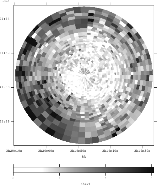
Figure 6: Temperature map of the perseus cluster core with 500 counts/cell. The counts were determined using the 14.9 ks exposure (see Sect. 3.2). The coordinates are J2000.

3.5 Spectra in small cells

In this section we finally use two grids of cells: firstly we determine the amount of absorption and the metallicities in cells with $\sim\,$9000 counts each using the model in eq. 1. We then subdivide these cells further until we obtain a grid with $\sim 500$ counts in each cell. In order to obtain cells that are not too elongated, we limit the ratio

$$q=\frac{(\alpha_{2}-\alpha_{1})\times(r_{1}+r_{2})/2}{r_{2}-r_{1}}$$ (2)

of cell width and depth (see Sect. 3.2) to be greater than $1/5$ and smaller than 5. The cells have a typical size (circle section at half radius) of 10 arcsec (5.2 kpc). In these fine cells we determine the temperature with a fixed metallicity at the value determined in the larger cells. This procedure yields the finely meshed temperature map shown in Fig. 6. The relative errors of the temperatures in this plot are of the order of $10-15$ per cent.

In order to obtain stable solutions for the absorption, we fix it to the median value $N_{\rm H}=0.143\times 10^{22}\hbox{${\rm\thinspace cm}^{-2}\,$}$ (Fig. 4) if it is smaller than $N_{\rm H}=0.16\times 10^{22}\hbox{${\rm\thinspace cm}^{-2}\,$}$, or otherwise fix it at the value determined in the first step; in total, there were only two cells where the local absorbing column densities of $N_{\rm H}=0.20\times 10^{22}$ cm^-2 and $N_{\rm H}=0.21\times 10^{22}$ cm^-2, respectively, had to be used. These two cells correspond to the region where the infalling high-velocity system is seen in absorption in the X-ray colour image by F00.

When looking at the goodness of the individual fits we noticed in a small number of cases that the assumed (fixed) metallicity appeared to underestimate the metallicity in these cells. In the cell with $r_{1}=43.39$ kpc, $r_{2}=46.43$ kpc, $\alpha_{1}=346^{\circ}$ and $\alpha_{2}=351^{\circ}$ (angles given in degrees, counterclockwise from north), for example, we found a reduced ${\chi_{\nu}}^{2}$ value of 1.3 when the metallicity was fixed at $Z=0.434$ solar. The reduced ${\chi_{\nu}}^{2}$ drops to 1.1 for the best fit $Z=2.87^{+1.60}_{-1.74}$ solar. The constraint is entirely due to the iron L complex. This also leads to an underestimate of the temperature: $3.8^{+0.60}_{-0.56}$ keV compared $4.57^{+0.53}_{-0.77}$ keV if the metallicity is left as a free parameter. Although the evidence is not statistically compelling, this may be due to small-scale inhomogeneities of the metallicity. However, currently the count rates on small scales are too low and accordingly the uncertainties too large to reliably determine metallicities on these scales.

In the temperature map the overall temperature distribution from Fig. 5 (middle panel) is again visible. In addition, the map includes fine detail showing prominently that the temperature is higher in the regions of the two inner and the north-western X-ray holes than in their surroundings. Extending from the bright rim to the south-east of the central X-ray holes the low-temperature (2 to 3 keV) gas extends westwards and spirals around counter-clockwise. This spiral shape of the colder gas corresponds to the swirly appearance of the 0.5 to 7 keV emission shown in Fig. 1. The shape of lines of constant temperature at radii $\sim 80$ kpc (2.6 arcmin) discussed in Sect. 3.4 are also seen here to be similar to the shape of the surface brightness drop in the X-ray emission. The general spiral appearance of the cooler X-ray gas in the core was also noted by F00 in their X-ray colour image; the shape of the temperature distribution and the overall magnitude of the temperatures in the cluster core as determined with X-ray colours by F00 are confirmed by our individual spectral fits.

4 Spectral deprojection

4.1 Azimuthally averaged profiles

In the previous sections we have treated the cluster as a two-dimensional object in order to learn about the overall spectral properties. Since complicated projection effects must be present due to the different locations of, for example, bubbles, brightness drops or metals in the cluster, we attempt in this section to unravel some of the projection effects that are present. However, this can only be done by assuming a specific symmetry.

We deproject the observed spectra, in particular the temperature profile (Fig. 2) and the metallicity profile (Fig. 3), by assuming spherical symmetry and using the projct model available in XSPEC combined with our standard APEC model (eq. 1). In order to reduce the number of parameters, only eight annuli with $\sim 144,000$ counts each were used (as measured in the January 2000 image).

The model assumes eight spherical, concentric shells filled with gas with independent temperatures and metallicities. The projct model adds the APEC spectral contributions from the X-ray emission in the shells in order to model each of the eight observed annular spectra. All eight spectra are fitted at the same time. Consistent with Fig. 4, we find no excess absorption except for the innermost region. With the current model and due to the complicated shape of the absorbing area (F00), however, it is not possible to determine in which shell the absorbing material is located.

The final deprojected temperature and metallicity profiles are shown in Fig. 7. We plot the deprojected values with solid error bars, while the temperatures and metallicities determined from the projected spectra are plotted with dotted error bars. Starting from the outside, the temperature profile drops very quickly in the first bin and continues to drop monotonically, but with a shallower slope afterwards. Also starting from the outside, the metallicity gradient appears to be steeper down to $\sim 70$ kpc than it was for the projected spectra, but is very similar, albeit with larger error bars, within 70 kpc. Inside a radius of $\sim 70$ kpc, we find the metallicity approximately constant at $Z\sim 0.5$ solar.

The X-ray data also allow us to determine the emission measure ${\rm EM}=n_{\rm e}^{2}\times V$ (via the normalization constant $K$ in eq. 1), where $n_{\rm e}$ is the electron density and $V$ the volume of the gas. Assuming that isothermal X-ray gas at the deprojected temperature $T$ fills the spherical shells, we can determine the pressure $p$ of the electrons, $p=n_{\rm e}\,$k$\,T$, as shown in Fig. 8. Note that the sudden rise in pressure in the last bin is an edge effect due to our assumption that there is no cluster emission outside this radius. Similarly, the steep deprojected temperature drop in the outermost bin of Fig. 7 is an artifact since the cluster extends significantly beyond the outermost radius accessible to the ACIS-S3 detector used. This is also apparent from the fact that the deprojected temperature value is best-fit higher than the projected value. The temperature, metallicity and emission measure values further in, however, will not be affected by this due to the steep brightness increase (see Fig. 5, left panel) towards the nucleus.

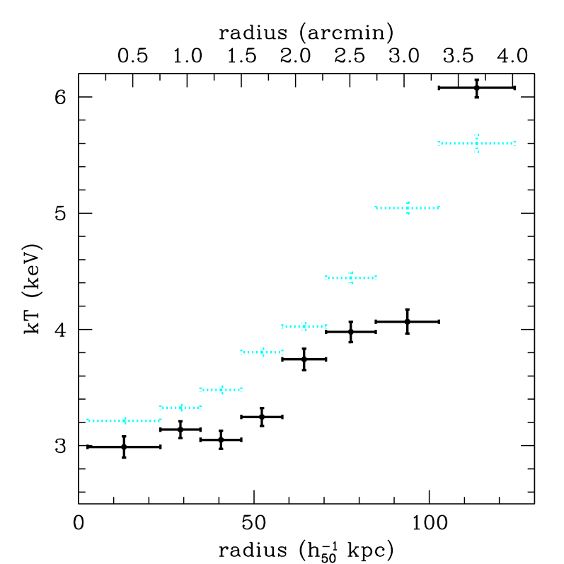
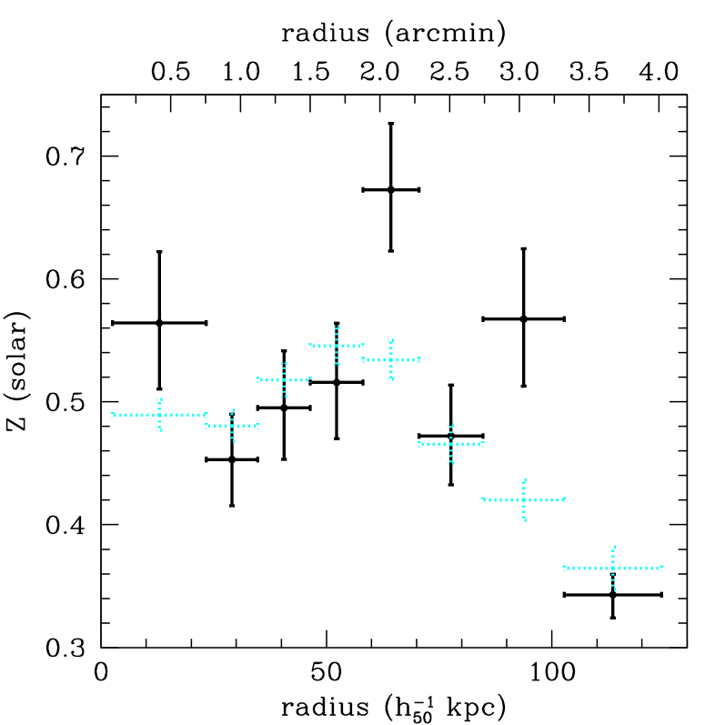
Figure 7: Deprojected temperature (left panel) and metallicity profiles (right panel) of the Perseus cluster core (solid lines). Also plotted with dotted lines are the corresponding projected quantities that are shown in Figs. 2 and 3 with higher resolution.

Figure 8: Electron pressure profile as determined using a spectral deprojection of the Perseus cluster core. The sudden rise in pressure in the outermost bin is not real, but an edge effect due to our data analysis (see text).

4.2 The X-ray emission from the X-ray holes

In the projected temperature maps we found that the spectra extracted from the two central X-ray holes as well as the western X-ray hole are best-fit by hotter and more metal rich gas than their immediate surroundings. It is possible that this is due to a projection effect, whereby we would be seeing the hot gas above and below an empty cavity.

In order to investigate the properties of the X-ray gas that fills the region of the holes, we have carried a local deprojection analysis. We have spectrally deprojected the emission emitted by 9 annular segments (Sect. 3.2) with azimuthal boundaries $\alpha_{1}=350$ degrees and $\alpha_{2}=28$ degrees and 14000 counts per segment (as measured in the January 2000 image) in the 0.5 to 7 keV band. The innermost segment occupies the region of the northern inner X-ray hole with radii between 5 and 27 arcsec of the nucleus. The analysis was analogous to the full-circle analysis in the last section, except that the absorption was forced to be the same for all segments and the metallicity in the inner hole was fixed at $Z=0.5$. The best-fit absorption was $N_{\rm H}=1.40\times 10^{21}$ ${\rm cm}^{-2}$, the reduced $\chi^{2}$ of the best fit was $\chi^{2}_{\nu}=1.14$.

Interestingly, we find that almost the entire projected emission in the innermost segment can be explained by the emission from the shells above. In Fig. 9 we show the allowed 68% ($1\;\sigma$), 95.4%($2\;\sigma$) and 99.73%($3\;\sigma$) confidence contours in the temperature/electron density plane of the parameters for an APEC component in the innermost segment. It can be seen that only a very low density plasma is allowed by the analysis. Since the emission measure constrained by the observed X-ray data is proportional to the volume of the gas, the allowed electron densities depend on the filling factor $f$ of the X-ray gas in the hole. We thus show the lines of pressure equilibrium with the second volume segment for three different filling factors of the X-ray gas (the electron pressure in the deprojected second segment is $p=n_{\rm e}\,T=0.17\,{\rm keV\,cm}^{-3}$, slightly higher than the shell-averaged pressures given in Fig. 8). These data rule out at $3\sigma$ the presence of X-ray gas at a temperature lower than 11 keV filling the entire X-ray hole. At the same confidence level we can rule out intracluster gas at the virial temperature of the cluster ($\sim$6.5 keV), filling one third of the X-ray hole.

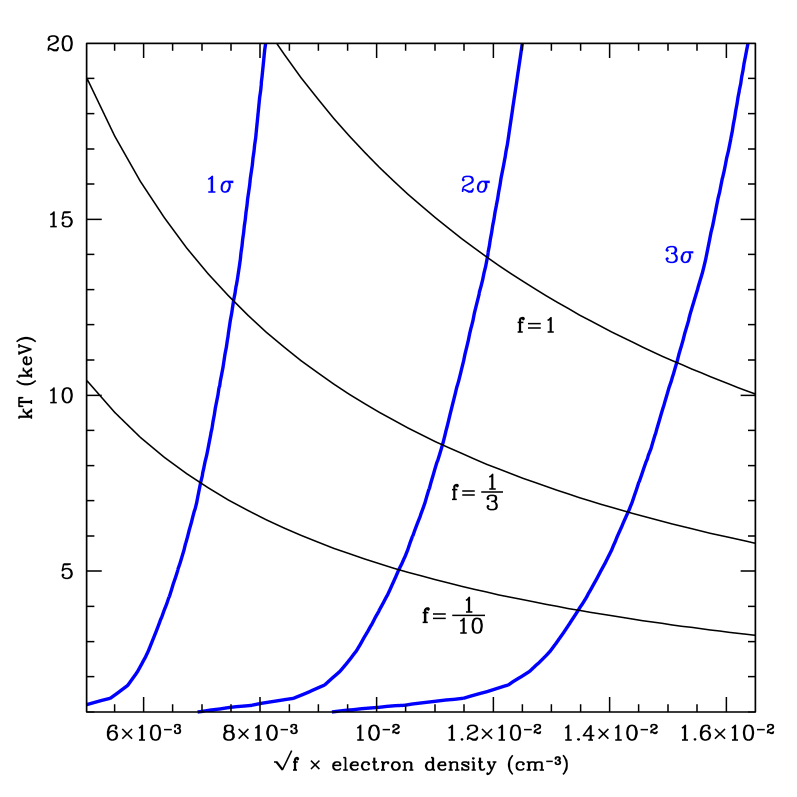
Figure 9: 68% ($1\;\sigma$), 95.4%($2\;\sigma$) and 99.73%($3\;\sigma$) confidence contours (thick lines) on the presence of an isothermal APEC component in the northern inner X-ray hole. The hyperbolas (thin lines) denote the required parameter pairs for pressure equilibrium with the X-ray gas at larger radii, assuming filling factors $f=\frac{1}{10}$, $f=\frac{1}{3}$ and $f=1$ of the X-ray gas.

5 Discussion

We have presented in this paper the results from a detailed temperature and metallicity mapping of the Perseus cluster core using Chandra observations.

We work with the complete useful ACIS-S data set comprising a total of 23.9 ks. Beginning by averaging over large annuli around the nucleus, we find that the temperature averaged in such annuli rises smoothly from $\sim 3.0$ keV to $\sim 5.5$ keV at 120 kpc. A small kink is found, however, in this profile at $\sim 80$ kpc, which corresponds to a surface brightness drop seen in the X-ray image. Using solar abundances according to Anders & Grevesse (1989), the metallicity rises from $Z\sim 0.4$ solar with decreasing radius to a maximum $Z\sim 0.6$ solar at $\sim 60$ kpc. There may be a peak of the metallicity profile at $\sim 50-60$ kpc, which is reminiscent of such peaks in other clusters (e.g., Sanders & Fabian, 2001). However, inside 60 kpc the metallicity varies little, with a central metallicity of $Z\sim 0.5$ solar. We have also carried out a spectral deprojection analysis of the radially averaged profile, which yields a very similar picture.

Spatially resolved spectroscopy in small cells shows that the temperature distribution in the Perseus cluster is not symmetrical. In fact, the distribution of cold ($2-3$ keV) gas in the centre appears to spiral outward and corresponds to the swirly appearance of the X-ray emission (see Figs. 1 and 6). This may suggest the presence of angular momentum of the intracluster gas (F00). There are, however, other possibilities, such as the model by Churazov et al. (2000) (see also their adaptively smoothed ROSAT image) who propose that rising radio bubbles (such as the X-ray holes) are responsible for the overall spiral structure. The outer surface brightness drop is traced by a rise in temperature (with increasing radius). This is reminiscent, although not as large, of the temperature drop at the cold front seen by Markevitch et al. (2000). If thermal conduction is an important effect in the intracluster medium, such fronts could reflect the magnetic field structure.

A comparison of the metallicity distribution with the galaxy distribution from an optical image from the Digital Sky Survey does not show any obvious correlation between the galaxies and regions of higher metallicity. Projection effects and the resolution of the Chandra metallicity map, however, do not allow to rule out any correlation yet.

We find that the spectra extracted from the two central X-ray holes as well as the western X-ray hole are best-fit by hotter and more metal rich gas than their immediate surroundings. Using a spectral deprojection under the assumption of spherical symmetry in a sphere segment containing the northern inner X-ray hole, we have tested whether this could be due to a projection effect. Interestingly, we find that most of the X-ray emission in the hole can be explained by the projected emission of the shells further out. This directly addresses the issue of the X-ray gas content of the X-ray holes mentioned in the introduction; we find tight limits on the presence of an isothermal component in the X-ray hole, ruling out volume-filling X-ray gas with temperatures below 11 keV at 3$\sigma$.

The temperature distribution of the gas in the vicinity of the X-ray holes is of great importance for theories of radio source heating to counter the short cooling time of the X-ray gas in this cluster (e.g., F00). Longer exposure times are needed to reveal if there is cool gas associated with the wake of the bubble, as, for example, in the model by Churazov et al. (2000), who proposed that the radio bubbles would transport cooler gas from the cluster centre ‘upwards’. The bubbles may also transport or drag metals upwards. The subject of radio bubbles and their interaction with the intracluster gas has recently become the subject of much work (Churazov et al. 2001; Brüggen & Kaiser 2001; Quilis, Bower & Balogh 2001; McNamara et al. 2001; F02). The Chandra results provide essential observational input to test these theories.

References

- Allen et al. (2001) Allen S.W., Fabian A.C., Johnstone R.M., Arnaud K.A., Nulsen P.E.J., 2001, MNRAS, 322, 589
- Anders & Grevesse (1989) Anders E., Grevesse N., 1989, Geochimica et Cosmochimica Acta, 53, 197
- Arnaud (1996) Arnaud K.A., 1996, Astronomical Data Analysis Software and Systems V, eds. Jacoby G. and Barnes J., p17, ASP Conf. Series volume 101
- Balucinska-Church & McCammon (1992) Balucinska-Church M., McCammon D., 1992, ApJ, 400, 699
- Blundell et al. (2000) Blundell K., Kassim N., Perley R., 2000; preprint astro-ph/0004005
- Böhringer et al. (1993) Boehringer H., Voges W., Fabian A.C., Edge A.C., Neumann D.M., 1993, MNRAS, 264, L25
- Briggs et al. (1982) Briggs S.A., Snijders M.A.J., Boksenberg A., 1982, Nature, 300, 336
- Brüggen & Kaiser (2001) Brüggen M., Kaiser C.R., 2001, MNRAS, 325, 676
- Churazov et al. (2000) Churazov E., Forman W., Jones C., Böhringer H., 2000, A&A, 356, 788
- Churazov et al. (2001) Churazov E., Brüggen M., Kaiser C.R., Böhringer H., Forman W., 2001, ApJ, 554, 261
- Conselice et al. (2001) Conselice C.J., Gallagher J.S., Wyse, R.F.G., 2001, AJ, 122, 2281
- de Young et al. (1973) de Young D.S., Roberts M.S., Saslaw W.C., 1973, ApJ, 185, 809
- Dickey & Lockman (1990) Dickey J.M., Lockman F.J., 1990, ARAA, 28, 215
- Fabian et al. (1981) Fabian A.C., Hu E.M., Cowie L.L., Grindlay J., 1981, ApJ, 248, 47
- Fabian (1994) Fabian A.C., 1994, ARA&A, 32, 277
- Fabian et al. (2000) Fabian A.C., et al., 2000, MNRAS, 318, L65 (F00)
- Fabian et al. (2002) Fabian A.C., Celotti A., Blundell K.M., Kassim N.E., Perley R.A., 2002, MNRAS, 331, 369 (F02)
- Giovannini et al. (1998) Giovannini G., Cotton W.D., Feretti L., Lara L., Venturi T., 1998, ApJ, 493, 632
- Heinz et al. (1998) Heinz S., Reynolds C.S., Begelman M.C., 1998, ApJ, 501, 126
- Kaastra & Mewe (1993) Kaastra J.S., Mewe R., 1993, Legacy, 3, 16
- Liedahl et al. (1995) Liedahl D.A., Osterheld A.L., Goldstein W.H., 1995, ApJ, 438, L115
- Lynds (1970) Lynds R., 1970, ApJL, 159, L151
- Markevitch et al. (2000) Markevitch M., et al., 2000, ApJ, 541, 542
- McNamara et al. (1996) McNamara B.R., O’Connell R.W., Sarazin C.L., 1996, AJ, 112, 91
- McNamara et al. (2001) McNamara B.R., et al., 2001, ApJL, 562, L149
- Quilis et al. (2001) Quilis V., Bower R.G., Balogh M.L., 2001, MNRAS, 328, 1091
- Sanders & Fabian (2001) Sanders J.S., Fabian A.C., 2001, MNRAS, 325, 178
- Unger et al. (1990) Unger S.W., et al., 1990, MNRAS, 242, 33P