Long-term photometric behaviour of XZ Dra

The extended photometry available for XZ Dra, a Blazhko type RR Lyrae star, makes it possible to study its long-term behavior. It is shown that its pulsation period exhibit cyclic, but not strictly regular variations with $\approx 7200$ d period. The Blazhko period ($\approx 76$ d) seems to follow the observed period changes of the fundamental mode pulsation with ${\rm d}P_{\rm B}/{\rm d}P_{0}=7.7\times 10^{4}$ gradient. Binary model cannot explain this order of period change of the Blazhko modulation, nevertheless it can be brought into agreement with the $O-C$ data of the pulsation. The possibility of occurrence of magnetic cycle is raised.

1 Introduction

One of the unsolved problems, which is perhaps the most intriguing one in RR Lyrae star research, is the Blazhko effect, the amplitude and/or phase modulation of light curves with periods of $10-500$ days. Although theoretical interpretations of the phenomenon have been suggested (Shibahashi, 2000; Van Hoolst, 2000), a clear explanation of it is still lacking.

Blazhko (1907) was the very first who recognized that the light maximum of an RR Lyrae star (namely RW Dra) showed phase modulation on a long time-scale (around 40 days). Subsequent investigation has revealed that the phase modulation is accompanied by modulation of the light curve and the amplitude of light variation. About a third of the fundamental mode RR Lyrae stars show the effect (Szeidl, 1988), however, only few have been investigated in detail yet. There are less than 10 galactic field stars which have sufficient observations to permit deeper insight into their Blazhko properties, but these studies have not been enough to expose the physical background of the observed modulation. The number of Blazhko stars which have been observed for a long enough time to detect any changes in their modulation properties is even fewer. Most of the stars listed in the summary review paper of Blazhko variables (Szeidl, 1988, completed in Smith 1995) still have not been studied in detail.

XZ Dra (BD$+64\degr 1332$, HIP 94134, $\alpha_{2000}=19^{\rm h}09^{\rm m}42\aas@@fstack{s}6$, $\delta_{2000}=+64\degr 51\arcmin 32\arcsec$) is one of the best observed RRab stars. Schneller (1929) discovered the star’s variability on Babelsberg plates. Soon after the announcement of the discovery, Beyer (1934) observed the star visually and determined the correct value of the fundamental period. He also commented on the strong oscillation in brightness of the individual light maxima. Balázs & Detre (1941), based on the rough estimates of their photographic observations showed that these oscillations had a period of 76 days and the star’s behaviour resembled that of AR Her.

During the last century, continuous effort has been made at the Konkoly Observatory to regularly observe RR Lyrae stars with Blazhko effect. Collection of photometric and some radial velocity observations of XZ Dra has been recently published in Szeidl et al. (2001). These data, together with all the published measurements of XZ Dra, made it possible to follow its photometric behaviour during a remarkably long (70-year) period. Due to the extended data now available a detailed analysis of the properties of its pulsation and Blazhko behaviour has become feasible.

2 The data

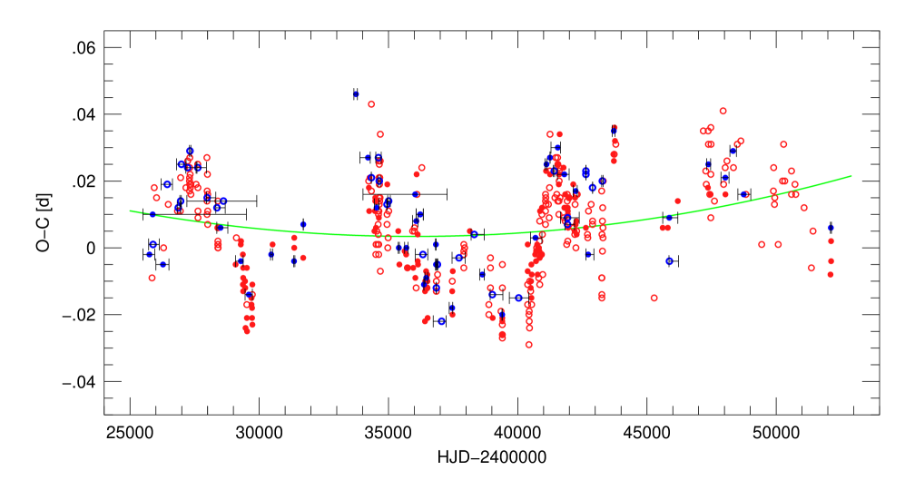
Figure 1: $O-C$ diagram of XZ Dra constructed from individual (red) and normal (blue) maxima compiled in Szeidl et al. (2001). Filled symbols are for professional photographic, photoelectric and CCD observations. Open symbols show visual and amateur data, and also all the uncertain observations noted by colon in Szeidl et al. (2001). Horizontal bars indicate the time span of the observations the normal maxima were derived from. The green line is the least square parabolic fit to all the data.

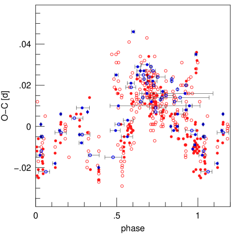
Figure 2: $O-C$ data folded with $7200$ d. Symbols are the same as in Fig. 1, the parabolic fit to the data has been extracted. The maxima and the decline phases of the $O-C$ seem to be closely repetitive, but at around minimal values, the long-term changes have a much more irregular character.

Both the extended photometric and the scarce radial velocity observations available for XZ Dra have been utilized in the present study. The photometric data used are the photoelectric, CCD, photographic and visual observations collected in Szeidl et al. (2001) and also all the other published photometries. A complete reference list of all the available photometric data of XZ Dra were also given in Szeidl et al. (2001).

In order to obtain the best possible time coverage of the observations the different types of measurements were combined if they could be reliably transformed to the same magnitude scale and if they belonged to a time interval for which data were analyzed together. Thus $B_{\rm pg}$ and $V_{\rm pg}$ (photographic) data were transformed to $B_{\rm pe}$ and $V_{\rm pe}$ (photoelectric) magnitudes, respectively, by correcting for zero point offsets. We note, however, that only very few and scarce photographic measurements (Zaleski, 1965; Harding & Penston, 1966) were transformed in this way, as for most part of the photographic data there were no contemporary photoelectric observations. The visual observations were treated separately, simultaneous visual observations were linearly transformed to gain a common magnitude scale.

The most deviant points were omitted from each of the data sets.

If there were no observations during the descending part of the light curve (typically that was the case in the photoelectric data and also in some parts of the photographic observations) $5-15$ artificial data were added in order to ensure the stability of the light curve solutions. The small number of artificial data compared to the total number of the real observations provided that the results were not biased by the actual choice of the artificial data.

When analyzing the magnitudes of maxima, all the observations of the same wavelength were combined in order to obtain the best possible time coverage. For this purpose the $V$ and visual magnitudes of maxima were also combined by simply correcting for zero point shifts between the $V_{\rm pe}$, $V_{\rm pg}$ and the visual data.

A complete list of individual and normal maximum timings (an average maximum timing determined from observations of more than one pulsation cycle taking into account the whole light curve as well not only times of maxima) and $O-C$ values using the ephemeris

$${\rm Max(HJD)}=2\,431\,244.383+0.4764955\,E$$ (1)

were also given in Table 10.a and 10.b of Szeidl et al. (2001). In the present paper these $O-C$ data are also elaborated.

Although only very limited radial velocity observations of XZ Dra are available, these observations are also reviewed (Sect. 4.3) in comparison with the possible explanations of the photometric data.

3 Period changes

The collection of all the individual and normal maximum timings of XZ Dra allows us to follow its period changes using a nearly continuous data base covering 70 years. The $O-C$ diagram constructed from this compilation is shown in Fig. 1. According to Fig. 1 the mean pulsation period of XZ Dra has not changed significantly during the time covered by observations, but $O-C$ variations ranging $0.02-0.04$ d in $2000-5000$ d intervals indicate that opposite sign period changes of the order of $10^{-5}$ d/d have been occurring.

A detailed inspection of the $O-C$ data exposed that besides a small continuous period increase, a $\approx 7200$ d cyclic variation can be also detected. In Section 3.1 these long-term changes are documented. Thorough analysis of all the available photometric observations have been performed in Section 3.2, with a special focus on the possible changes in the Blazhko properties consequent to the detected variations of the pulsation period.

3.1 Long-term and sudden period changes

Fourier analysis of the $O-C$ data shown in Fig. 1 revealed that the period change behaviour of XZ Dra can be described with a $\approx 7200$ d asymmetric shape periodic modulation. Filtering out this cycle, it becomes evident that a slight, continuous period increase has also occurred, as the residual $O-C$ clearly has a parabolic shape. In Fig. 1 the parabolic fit to the data is also shown. According to the parameters of the quadratic fit the ephemeris of XZ Dra has been modified to:

$$\begin{split}{\rm Max(HJD)}=2\,435\,819.2190(9)+0.47649550(6)\,E+\\ 1.9(3)\times 10^{-11}\,E^{2}\end{split}$$ (2)

The continuous period change corresponds to $2\times 10^{-6}$ d period increase during the 25 000 days covered by the observations. As this period change is negligible if compared to the much more effective, shorter time-scale period changes, in the course of the analysis performed in Section 3.2 this continuous period increase has been ignored.

In order to document the cyclic nature of the long-term variability seen in Fig. 1, the $O-C$ data, after removing the parabolic fit, is folded with 7200 d in Fig. 2. The best period found by fitting a sinusoid with 2 harmonics to the data is $7198\pm 100$ d. The maxima and the descending parts of the $O-C$ data follow this periodicity well, but the larger scatter of the folded curve around minimum and ascending branch indicates that there are differences in the shape of the $O-C$ changes from one cycle to the other.

It is also important to note that besides the parabolic and the 7200 d cyclic variations of the $O-C$ there are also sudden changes observed, see e.g. the $0.02$ d increase around HJD 2 443 800.

3.2 Pulsation and Blazhko periods

The observed changes in the pulsation period raise the issue of the concurrent behaviour of the Blazhko modulation. An obvious way to follow the possible variations of the Blazhko period is to construct the $O-C$ diagram corresponding to the Blazhko periodicity. Such an attempt has, however, failed. The time coverage of the observations, and the not strictly regular nature of the Blazhko modulation, in most of the cases permit only an estimation of the observed times of maxima of the Blazhko cycles with $5-15$ days accuracy. To draw firm conclusions about smaller period changes this accuracy is not enough. We thus mention only that all the $O-C$ values of the maximal phases of the Blazhko period spread within a 15 days range if calculated using a 75.7 d mean Blazhko period value.

We studied the simultaneous properties of the two periodicities using all the available photometric observations. The data were not corrected for the continuous period change shown in Sec. 3.1, because of its negligible effect along the time intervals of the analyzed data sets.

First, the data were divided into different segments according to the structure of the $O-C$ diagram. Linear parts of the $O-C$ were selected, assuming that along these segments no significant period change has been occurring. From different trial divisions of the data it turned out, that the folded light curves of those data sets which could definitely be described with a constant pulsation period value, always had a fix point in their rising branch. This behaviour of the modulation was also a guide in selecting data groups, considered not being biased by period change that mimics phase modulation.

Both the full light curves (Section 3.2.1) and the data of maximum timings and magnitudes (Section 3.2.3) were analyzed.

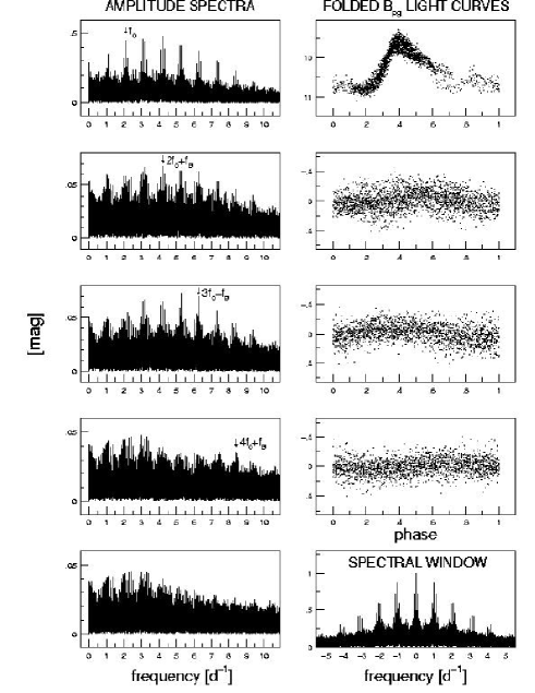
Figure 3: Fourier spectra and folded light curves of the photographic observations between JD 2 429 084 and JD 2 429 734 in the course of prewhitening first with the fundamental mode period and its harmonics then with frequencies corresponding to one of the possible modulation frequencies appearing in the consequent prewhitened spectra ($2f_{0}+f_{\rm B}$, $3f_{0}-f_{\rm B}$, $4f_{0}+f_{\rm B}$). These frequencies are indicated by arrows in the spectra and the residual light curves are folded according to these periods.

Table 1: Trial modulation frequency combinations used to fit the Hipparcos (ESA, 1997) (H1, H2 fits) and Dyachenko (1982) (D1, D2 fits) data. Besides the modulation frequencies listed, 5 and 4 harmonics of the pulsation frequency were also taken into account in the H1, H2 and D1, D2 fits, respectively. The $P_{0}$, $P_{\rm B}$ periods correspond to the minimum of the two dimensional rms distributions (see also Figs. 4 and Fig. 5).

H1 fit H2 fit D1 fit D2 fit

$$P_{0}$$ [d] 0.4764950 0.4764950 0.4765035 0.4765030

[d] 75.7 76.1 77.9 78.0

mod. fr. Amplitudes [mag]

0.0239 0.0255 0.0750 0.0676

0.0338 0.0311 0.0036

0.0243 0.0622 0.0364

0.0200 0.0226 0.0298

0.0088 0.0551

0.0132 0.0240

0.0317

0.0268

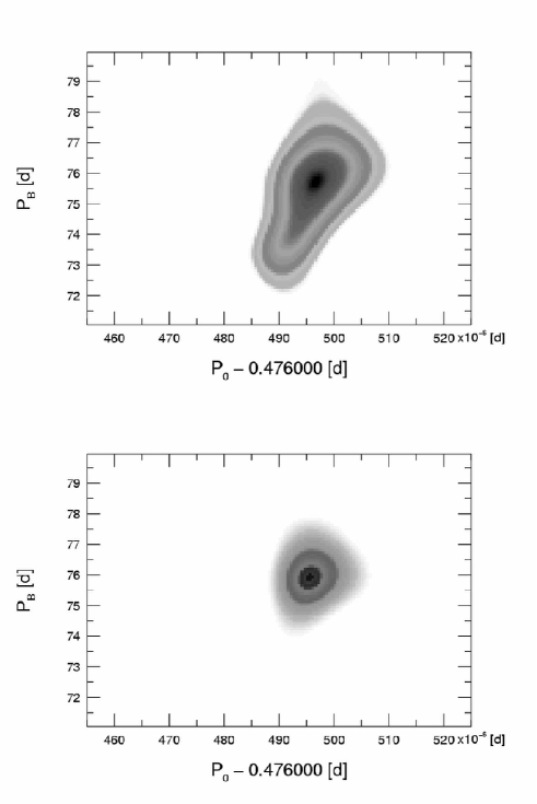
Figure 4: The rms scatter of the Hipparcos data on an arbitrary gray scale. Fits were calculated using pulsation and Blazhko periods indicated in the axes. The unit of the horizontal scale is $10^{-6}$ d. The pulsation frequency with 5 harmonics and modulation frequencies given in Table 1 were considered when determining the rms scatter of the fits. Solutions using modulation frequencies listed in Table 1 for H1 fit are shown in the upper, for H2 fit in the lower panels, respectively. The rms range shown is the increment of the minimal rms value by $\approx 10$%.

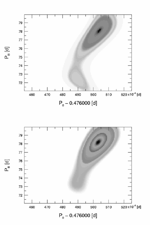
Figure 5: The same as in Fig. 4 but for Dyachenko (1982) visual observations. Solutions for D1 and D2 fits (Table 1) are shown in the upper and lower panels, respectively. $0.086-0.090$ mag rms range is shown in both panels.

3.2.1 Analyzing light curves

Different methods were used to determine the pulsation and Blazhko periods valid for the individual data sets. The governing principle was to find $f_{0}$ (fundamental mode frequency) and $f_{\rm B}$ (Blazhko frequency) that gave the best fit using $f_{0}$ and $4-8$ of its harmonics and $3-9$ additional frequencies among the modulation frequency pattern commonly found in the spectra of Blazhko variables: $k\times f_{0}\pm f_{\rm B}$ (k=1,2,3,4) and $f_{\rm B}$. Fourier decomposition using the MUFRAN program package (Kolláth, 1990), least square minimization technique and nonlinear regression facilities of Mathematica (Wolfram, 1996) have been used in deciding which modulation frequencies to take into account for the individual data sets, and to determine the actually valid $f_{0}$ and $f_{\rm B}$ frequencies.

In many cases it was not possible, however, to decide which modulation frequencies to take into account, as the shortness of the data set and/or its high noise, limited the parameter number of the solutions. In these cases many possibilities were tested and $f_{0}$ and $f_{\rm B}$ were only accepted if the same periods consistently appeared in the different solutions. Results with unreliable large amplitudes of the modulation frequencies were rejected.

Some examples of the applied procedure are documented in Figs. 3, 4, 5, 6, showing results for different data sets.

Due to the shortness and inconvenience of the data sampling of most of the data sets, their Fourier spectra are usually crowded by alias peaks which make it difficult to identify the real frequencies. At least one of the possible modulation frequencies, however, can be always detected in the spectra. Interestingly, this dominant modulation frequency is usually found near the higher harmonics ($2-4$) of the fundamental mode frequency. We do not know at present whether this is a real feature of the modulation, or this arises from the bias of the unfavourable data distribution.

The Fourier analysis of some data sets with good phase coverage can be also misleading in some cases. For example, the Fourier spectrum of the photographic data between JD 2 430 433 and JD 2 431 708 shows modulation frequencies at 0.0187 and 0.0243 c/d (53.5 and 41.2 d) distant from the harmonics of the pulsation frequency, which might be aliases of the true modulation peaks. Notwithstanding this, least square fit using 8 symmetrically placed modulation frequencies indicates better, more reliable solutions at 0.01302 and 0.01328 c/d (76.8 and 75.3 d).

A sample Fourier spectra of the photographic observations between JD 2 429 084 and JD 2 429 734 is shown in Fig. 3. The procedure of first prewhitening with the fundamental mode period (with 6 harmonics), then with the modulation frequencies appearing in the subsequent whitened spectra is documented in the left panels. The right panels show the folded light curves using the periods indicated by arrows to the corresponding spectra.

Fig. 4 and Fig. 5 show the two dimensional residual scatter of the Hipparcos (ESA, 1997) and Dyachenko (1982) light curves fitted by two different ‘Blazhko type’ frequency patterns listed in Table 1. For each possible $P_{0}$ and $P_{\rm B}$ pairs the rms residuals are shown in an arbitrary gray scale to set off the rms distribution in the vicinity of the best solution. It can be seen in Fig. 4 and Fig. 5 that the structure of the minimum places changes significantly for the different frequency solutions of a given data set but the location of the absolute minimum place remains very closely at the same $P_{0}$ and $P_{\rm B}$ period pair. Table 1 lists the modulation frequencies that were taken into account when calculating the rms of the fits shown in Figs. 4,  5, and their amplitudes at $P_{0}$ and $P_{\rm B}$ periods of the absolute minimum places. It is worth noting that the amplitudes of the same modulation frequency differ by as much as $30-50\%$ if different frequency patterns are used. This result indicates, that any speculation concerning possible amplitude changes of a given modulation frequency has to be taken with caution.

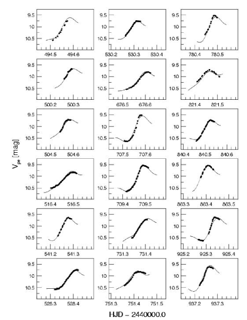
Figure 6: Photoelectric $V_{\rm pe}$ light curves fitted with $f_{0}$ (and 6 of its harmonics), $2f_{0}+f_{\rm B}$, $3f_{0}+f_{\rm B}$, $4f_{0}-f_{\rm B}$ frequencies using $P_{0}=0.476516$ d and $P_{\rm B}=76.69$ d determined from nonlinear regression to the data.

Table 2: Pulsation and Blazhko periods derived from the light curves

JD $$P_{0}$$    error    error source refs.

[d]     [d] [d]

0.476502 2 76.77 0.43 vis. 1,2,3

0.476491 1 76.19 0.23 1

0.476485 1 74.74 0.35 1

0.476495 2 75.27 0.30 1

0.476495 2 76.80 0.25

0.476462 4 73.73 0.55 1,4

0.476483 3 73.00 1.40 vis. 5,6

0.476499 2 76.64 0.37 1,4

0.476491 3 76.13 0.59 vis. 7

0.476493 1 75.79 0.05 , 1,4,8

0.476493 0.5 75.80 0.05 , 1,4,8,9

0.476487 3 75.59 0.65 vis. 7

0.476515 1 76.75 0.42 1

0.476514 1 76.40 0.45 1

0.476489 1 75.60 0.14 1

0.476489 1 75.61 0.15 1

0.476503 5 78.04 1.13 vis. 10

0.476496 3 75.90 1.25 11

References: 1 Szeidl et al. (2001), 2 Beyer (1934), 3 Lange (1938), 4 Zaleski (1965), 5 Batyrev (1955), 6 Klepikova (1958), 7 Lebedev (1975), 8 Sturch (1966), 9 Harding & Penston (1966), 10 Dyachenko (1982), 11 ESA (1997)

• Two Blazhko periods are equally possible

The photoelectric observations seriously lack measurements taken during the descending branch of the light curves. It makes direct Fourier analysis almost impossible, but nonlinear regression assuming appropriate frequencies can still yield reliable solution for $P_{0}$ and $P_{\rm B}$. For this purpose the nonlinear regression facilities of Mathematica assuming trial modulation frequency combinations were used. Fig 6 demonstrates such a result, photoelectric $V$ observations of the JD $2\,440\,494-2\,440\,937$ period are fitted with $f_{0}$, $2f_{0}+f_{\rm B}$, $3f_{0}+f_{\rm B}$, and $4f_{0}-f_{\rm B}$, that was found, after many trials using different possible modulation frequencies, as a reliable solution.

Periods obtained during the course of the above procedure for the different time intervals (supposed not to be affected by period changes), are summarized in Table 2. The periods determined for the time intervals given in Column 1 are the average values of different solutions, while estimating their errors both the range of the period values obtained and their individual errors are taken into account.

3.2.2 Periods determined from maximum timings and magnitudes

In Table 3 periods determined from maximum timings and magnitudes are listed. $V$ band ($V_{\rm pe}$, $V_{\rm pg}$ and visual after transformed to approximately match the $V_{\rm pe}$ magnitudes), $B$ band ($B_{\rm pe}$, $B_{\rm pg}$) maximum magnitudes and $B-V$ photoelectric observations of maxima were used independently. The $B-V$ maxima were determined from the Konkoly photoelectric $B$ and $V$ observations. $B-V$ curves were constructed by extrapolating the observations to the same instants, and the maxima of the colour curves were determined instead of taking $B_{\rm max}-V_{\rm max}$ values.

These data were also divided into segments corresponding to linear parts of the $O-C$ curve, however, the time intervals selected were not exactly identical to those chosen in Sect. 3.2.1.

The Blazhko periods were determined from single sinusoidal fits to the maximum magnitude values while the simultaneous pulsation periods were obtained from linear fits to the maximum timings, i.e. the $O-C$ values (Szeidl et al., 2001, Table 10.a) of the time interval considered. From the slope of the $O-C$ curve it was determined what the instantaneous pulsation period actually was.

Table 3 lists $P_{0}$ and $P_{\rm B}$ for the different time intervals determined this way. Cols. $1-3$ give the starting and ending dates of the $O-C$ data the pulsation period was calculated from, the $P_{0}$ period obtained, and its error. Cols. $4-7$, Cols. $8-11$, and Cols. $12-15$ list similar data for the Blazhko period, determined from $B$, $V$, and $B-V$ maximum magnitudes, and also references of the photometries used.

Table 3: Pulsation and Blazhko periods derived from times and magnitudes of maxima

JD $$P_{0}$$     error JD    error refs. JD    error refs. JD    error refs.

[d]    [d] [d] [d] [d]

0.476501 1 77.46 1.03 1,2,3

0.476486 2 75.03 1.49 4

0.476482 3 73.52 0.83 1

0.476473 4 73.03 2.10 1

0.476502 4 77.18 2.31 1,5

0.476495 1 75.82 0.20 1,5,6 75.95 0.20 1,5,6

0.476516 3 77.26 0.90 1 76.30 0.98 1,7 78.10 1.80 1

0.476489 1 75.78 0.49 1 75.28 0.33 1,7 76.43 1.56 1

0.476512 2 75.88 2.22 1,8

References: 1 Szeidl et al. (2001), 2 Beyer (1934), 3 Lange (1938), 4 Klepikova (1958), 5 Zaleski (1965), 6 Fitch et al. (1966), 7 Wenske (1982), 8 Dyachenko (1982)

• $P_{\rm B}$ determined from combined $B_{\rm pg}$, $B_{\rm pe}$ maximum magnitudes

• $P_{\rm B}$ determined from combined $V_{\rm pg}$, $V_{\rm pe}$, visual maximum magnitudes

• $P_{\rm B}$ determined from $(B-V)_{\rm pe}$ maximum magnitudes

Figure 7: Maximum magnitudes folded with the best Blazhko periods found for the different data sets (top panels) and also with the mean 75.75 d Blazhko period value (bottom panels). Data sets with the shortest and longest Blazhko periods are shown. The $rms$ scatter of sine fits of the bottom plots are $20-30$% larger than in the case of the best solutions.

To demonstrate the reality of changes in the length of the Blazhko cycle the data sets of light maximum magnitudes corresponding to the shortest and longest modulation periods as given in Table 3 are shown in Fig. 7 folded according to the mean Blazhko period value (75.75 d) and with the best $P_{\rm B}$ found to be valid for the individual data sets. In each cases the $rms$ scatter of a sine fit to the data is $20-30$% larger if folded with the mean $P_{\rm B}$ value.

3.2.3 Relation between $P_{0}$ and $P_{\rm B}$

The Blazhko periods as a function of the pulsation periods determined for the different linear segments of the $O-C$ are shown in Fig. 8. Filled symbols denote results obtained from analyzing the light curves (Table 2) and open circles show the periods determined from maximum timings and magnitudes (Table 3). The large uncertainties of the periods are mostly due either to the unfavourable data sampling or the shortness of the analyzed data sets. The length of the linear parts of the $O-C$, however, seriously delimit the length of the data sets used to determine the actual period values.

Figure 8: Pulsation ($P_{0}$) vs. Blazhko ($P_{\rm B}$) periods of XZ Dra. Filled and open symbols represent data of Table 2 and Table 3, respectively. The linear fit to the data has a $7.68\times 10^{4}$ d/d gradient.

Both sets of data plotted in Fig. 8 indicate a linear correlation between the two periodicities. A least square linear fit to the combined data gives a $7.7\pm 1.1\times 10^{4}$ d/d slope of the regression line.

The fact that not only data around the extreme $P_{0}$ values indicate the correlation but the ‘mid points’ also follow a definite trend, strengthens the validity of the result, namely that in the case of XZ Dra, $P_{0}$ and $P_{\rm B}$ periods are not independent quantities but exhibit parallel changes.

Similar connected changes of the pulsation and Blazhko periods have been already suggested for XZ Cyg (LaCluyzé et al., 2002), RW Dra (Firmanyuk, 1978), and RV UMa (Kanyó, 1976). In these three stars, however, instead of parallel, reverse changes of the two periods are suggested.

Possible explanations of the phenomenon are given in Section 5.

4 The Blazhko variations

4.1 Stability of the Blazhko phase

Figure 9: Folded curves of maxima magnitudes using P=75.75 d mean Blazhko period. Panel a) shows $B_{\rm pe}$ (filled circles) and $B_{\rm pg}+0\aas@@fstack{m}4$ (open circles) data of the JD $2\,428\,404-2\,447\,462$ time interval. Panel b) shows $V_{\rm vis,pg,pe,CCD}$ maxima magnitudes transformed to the same magnitude scale (JD $2\,425\,850-2\,452\,100$), professional photoelectric and CCD observations are denoted by filled circles. c) In the panel showing $(B-V)_{\rm max}$ magnitudes only photoelectric observations are plotted, the less certain values obtained preceding JD 2 438 000 Szeidl et al. (2001) are denoted by open circles. Panel d) shows artificial maximum magnitudes which were generated by taking into account the observed Blazhko period changes. Each of the folded curves show relatively small scatter that indicates phase stability of the Blazhko modulation along the entire time interval covered by the observations.

The best studied Blazhko variable, RR Lyrae, shows pronounced cyclic behaviour of its Blazhko modulation. It can be described as a lowering of the amplitude of the modulation and a jump in the Blazhko phase in about every four years (Detre & Szeidl, 1973). On the contrary, XZ Dra shows surprising stability of the Blazhko phases during the entire time interval covered by observations, notwithstanding the changes of its Blazhko period.

In Fig. 9 all the observed maxima ($B_{\rm pg}$ and $B_{\rm pe}$ between JD $2\,428\,404-2\,447\,462$, and visual and $V_{\rm pe}$ between JD $2\,425\,850-2\,452\,100$) are shown. The $B-V$ maximum magnitudes are from photoelectric observations. The fact, that all these maximum magnitudes can be folded with a common Blazhko period indicates strong stability of the Blazhko phases.

The relatively small scatter of the folded curves of maximum magnitudes seems to contradict the detected changes of the Blazhko period (see section 3). In order to examine the phase incoherence of the maximum magnitudes induced by the detected Blazhko period changes, artificial data ($\rm{ART_{max}}$) were generated and treated similarly to true observations. Using the Blazhko periods listed in Table 2 and Table 3 for the different time intervals, artificial maximum magnitudes were generated for the JD $2\,425\,850-2\,443\,300$ interval supposing sinusoidal changes with varying period. Data sampling follows the distribution of the real observations and an arbitrary magnitude scale is used.

Although it is somewhat ambiguous which periods to use to fill the gaps in the observations, the simulation shows that the detected period changes do not give rise to large divergence in the Blazhko phases. The artificial maximum magnitudes, folded with the same Blazhko period as the measured instants of maxima, are shown in the bottom panel of Fig. 9. The scatter of the folded $\rm{ART_{max}}$ curve seems to be similar to that of the true observations, thus we can conclude that the phase stability does not contradict the period changes of the Blazhko modulation. We also recall that the light curve of the pulsation shows similar behaviour. The influence of the detected changes of the pulsation period on the folded light curve of the entire set of observations is not larger than phase shifts of about $10-15\%$ of the period, which means that all the photometric data can be folded with a mean pulsation period without larger phase incoherences.

4.2 Colour changes

The colour changes of Blazhko variables during their modulation cycles have not been studied in detail yet. Multicolour observations show that maximum magnitudes are bluer in the larger amplitude phase of the modulation. However, because of the lack of complete colour curves along the Blazhko cycle we still do not know whether these color changes are incidental to mean colour changes, or reflect only differences in the shape of the colour curves.

The photoelectric observations of Szeidl et al. (2001) also delimit us to detect only $B-V$ colour changes of light maxima. Fig. 9 shows the $B$, $V$ and $B-V$ magnitudes of maxima folded with the mean Blazhko period value (75.7 d). The $B$ and $V$ maximum magnitudes exhibit $0.2-0.3$ mag changes along the Blazhko period, while the amplitude of the $B-V$ colour of the maxima is about 0.06 mag, again, the colours of maxima are bluer in the larger amplitude phases of the Blazhko cycle.

As the sampling of the photoelectric data is not suitable for the investigation of possible colour changes of the minima or the mean colours, the interpretation of this result needs further multicolour observations of complete light curves along the entire Blazhko cycle.

4.3 Radial velocity changes

Three sets of radial velocity measurements of XZ Dra are available. Woolley & Aly (1966) published 9 radial velocity observations that covered the different phases of the pulsation within 11 days (JD $2\,438\,929-2\,438\,940$). According to the B and V magnitudes of maxima, this interval fell within the minimal amplitude phase of the Blazhko period. The mean value of these radial velocity measurements is $\langle V_{\rm rad}\rangle=-30.83\pm 1.56$ km/s, as defined by fitting the actual pulsation frequency (determined from the light curve) and 2 of its harmonics to the radial velocity data.

Radial velocity values obtained from spectra taken in 1971 with the 72 inch telescope of the Dominion Astrophysical Observatory, were published in Szeidl et al. (2001). These data were gathered during a longer time interval, and covered different phases of the Blazhko and the pulsation cycles as well. The typical error of these measurements was 5 km/s. Although radial velocity curves of Blazhko variables are different in the different phases of the Blazhko cycle, its mean values during the pulsation cycles are supposed to remain the same. Therefore, it seems plausible to use all these measurements to determine the actual mean value of the radial velocity, instead of selecting observations belonging to a given Blazhko phase, as that would result in a much more limited sample with much more uncertain mean value. Even if all the radial velocity measurements from 1971 are used, the phase coverage of the pulsation is not complete enough to fit a reliable radial velocity curve when determining its mean value. Adding 1-2 artificial data via polynomial interpolation helps the situation. The mean value of the so completed radial velocity data is determined similarly to that of Woolley’s data (i.e, by using 3rd order Fourier fit). As a result $\langle V_{\rm rad}\rangle=-32.0\pm 3.35$ km/s is obtained if uncertainty arising from the choice of the complementary data is also taken into account.

The third published data set of radial velocity observations of XZ Dra are the four measurements of Layden (1994) obtained around JD 2 448 131. Although these observations show synchronous changes with the photometric variations, which exclude misidentification, their mean value $+77\pm 22$ km/s is very discrepant from the other two mean radial velocity values. Although the individual errors of Layden’s measurements are very large, about 45 km/s, this cannot explain a systematic offset of about 100 km/s (Layden, 2001). We could not find any explanation for the deviation of these data, however, as no physical reason for such a large variation of the mean radial velocity seems to be plausible (see also Sect. 5.1), these data are regarded as unreliable.

As a summary we conclude in that the presently available radial velocity measurements are not enough to draw any firm conclusion about the occurrence of real changes in the mean radial velocity of XZ Dra. To detect radial velocity changes connected to the $O-C$ variations, further extended accurate radial velocity observations are required.

5 Possible explanations

5.1 Binary model

Light time effect in a binary system is a plausible explanation for a periodic $O-C$ diagram. Binaries, however, are extremely rare among RR Lyrae stars, and no indication of being a binary member has emerged previously for any Blazhko type RR Lyrae.

The binary orbit can be described by six parameters: the semi-major axis $a$, the eccentricity $e$, the inclination $i$, the argument of periastron $\omega$, the epoch of periastron passage $\tau$, and the position angle of the line of ascending node $\Omega$. The semi-major axis and the inclination are inseparable ($\xi=a\sin i$), and $\Omega$ cannot be determined at all in a non-eclipsing system.

Following Coutts (1971) we express the $O-C$ variation as a function of time with the orbital elements:

$$O-C=c_{0}+{\xi(e^{2}-1)\over{c}}\left[{{\cos\omega\sin\nu}\over{1+e\cos\nu}}-{{\sin\omega}\over{e(1+e\cos\nu)}}\right]\Bigg{|}^{\nu}_{\nu_{0}}$$ (3)

where $c$ denotes the speed of light, $c_{0}$ is the correction term to take into account the initial epoch from which the $O-C$ values have been calculated, $\nu=\nu(t)$ is the true anomaly (henceforward the notation of time dependence $t$ is omitted), and $\nu_{0}=\nu(t=\tau)$.

It is well-known that the two centre problem has no closed analytic expression for $\nu(t)$. We use the classical formulae (see $e.g.$, Winter, 1947):

$$\begin{split}\sin\nu&=\\ &2\sqrt{1-e^{2}}\sum\limits_{k=1}^{\infty}J^{\prime}_{k}(ke)\sin\left[k{{2\pi}\over{P_{\rm orb}}}(t-\tau)\right],\\ \cos\nu&=\\ &-e+{{2(1-e^{2})}\over{e}}\sum\limits_{k=1}^{\infty}J_{k}(ke)\cos\left[k{{2\pi}\over{P_{\rm orb}}}(t-\tau)\right],\end{split}$$ (4)

where $P_{\rm orb}$, $J_{k}$ and $J^{\prime}_{k}$ denote the orbital period of the binary, the Bessel function of first kind of order $k$, and its derivative, respectively, and also the recursion relation for Bessel function ($e.g.$ Abramowitz & Stegun, 1971):

$$J^{\prime}_{k}(x) = {1\over 2}\left[J_{k-1}(x)-J_{k+1}(x)\right].$$ (5)

To find the model parameters of the supposed binary system, we need to solve the non-linear least-squares problem defined by Eq. (3) and the $O-C$ data. The model fitting was carried out using the combined data set of both individual and normal maximum timings (422 points). These data are shown in Fig. 1 and Fig. 2 by red and blue symbols, respectively. The data was first corrected for the continuous period increase according to Eq. (2). Weight factors were 2 and 1 for normal and individual maxima, respectively.

Substituting Eqs. (4) into Eq. (3) we obtain an expression including six parameters ($\xi$, $e$, $\omega$, $\tau$, $P_{\rm orb},c_{0}$). In practice, we solved the problem of parameter estimation by a combination of grid search method (using $e$ as control parameter) and the Levenberg-Marquardt algorithm (Marquardt, 1963) by utilizing the facilities of the program package Mathematica. Sums truncated to $30-100$ elements had been proven to have sufficient accuracy and were calculated instead of infinite sums.

The parameter values obtained and the rms of the fits that characterize the goodness-of-fit are summarized in Table 4. We note that the time coverage of the $O-C$ data is much more complete than that of any similar data analyzed before. The only RR Lyrae for which binary model solution has been calculated is TU UMa, a non-Blazhko RRab star with $P_{0}=0.558$ d pulsation period, its binary model (Wade et al., 1999) is based only on 83 points. It is worth noting that both for XZ Dra and TU UMa, large eccentricity solutions have emerged ($e\approx 0.7-0.9$) and the orbital periods are also very similar, around 7100 and 8000 days, respectively.

Table 4: Results of binary model fitting

Parameter	Model
$e$	0.65		0.8		0.95
$P_{\rm orb}$[d]	$7113.8$	$\pm$ 51.2	$7097.8$	$\pm$ 42.4	$7013.3$	$\pm$ 9.66
$\xi$ [AU]	$-2.443$	$\pm$ 0.145	$-2.725$	$\pm$ 0.178	$-3.504$	$\pm$ 0.330
$\tau$ [JD]	$2427165.3$	$\pm$ 108.13	$2427174.3$	$\pm$ 80.86	$2427334.9$	$\pm$ 16.93
$\omega$ [rad]	$1.2885$	$\pm$ 0.074	$1.1531$	$\pm$ 0.082	$0.8778$	$\pm$ 0.097
$c_{0}$ [d]	$-0.01363$	$\pm$ 0.00111	$-0.01319$	$\pm$ 0.00107	$-0.01249$	$\pm$ 0.00102
$\sigma$ [d]	0.01404		0.01397		0.01399

Figure 10: Binary model solutions for the $O-C$ data assuming binary orbits of 0.65, 0.80, and 0.95 eccentricities. Upper panels show the $O-C$ data over plotted by the different eccentricity binary model predictions. Middle and bottom panels show similar plots of the pulsation period and radial velocity data, respectively. Period differences using $\overline{P_{0}}=0.4764955$ d mean pulsation period value are indicated and the time intervals that the observed periods correspond to are also shown. Although global agreement between the observations and the corresponding fits is achieved, significant differences can be also seen.

Although radial velocity data of XZ Dra are too few to make them useful in model-fitting, it is worth checking their values in comparison with the binary model solutions. Predictions for possible radial velocity changes are also useful in order to obtain successful observational evidence pro or contra the binary hypothesis. To estimate the $\gamma$ velocity we minimized the least-square sum in the deviations of the measured mean radial velocities ($\langle V_{\rm rad}\rangle$, see Sect. 4.3) from the fits. The so obtained $\gamma$ velocities ($-29.06,-28.99$ and $-29.39$ km/s for the 0.65, 0.80 and 0.95 eccentricity solutions, respectively) were subtracted from the measured mean radial velocity values ($v_{\rm rad(obs)}=\langle V_{\rm rad}\rangle-\gamma$) in order to compare them with the models.

The center-of-mass radial velocity can be calculated according to the formula:

$$v_{\rm rad}={{2\pi\xi}\over{P_{\rm orb}\sqrt{1-e^{2}}}}\left[\cos\omega\left(\cos\nu+e\right)-\sin\omega\sin\nu\right].$$ (6)

Substituting Eqs. (4) into Eq. (6) we arrive at a formula that expresses the radial velocity of the center-of-mass as a function of time.

Fig. 10 compares the observed $O-C$, pulsation period ($P_{0}(t)-\overline{P_{0}};\,\,\overline{P_{0}}=0.4764955$ d) and center-of-mass radial velocity values with predictions of three possible binary models listed in Table 4.

The three different eccentricity models shown are in similarly good agreement with the observations. However, both the $O-C$ and period data indicate significant differences as well. None of the models follows the very steep increase of the $O-C$ around JD 2 440 500, and there are also outlying observed period values according to each of the solutions.

The overall fitting accuracy of the $O-C$ is 0.014 d ($\approx$ 20 min) which also seems to be larger than expected. Although the Blazhko modulation accounts for some real scatter of the $O-C$ data, data analysis indicates that the $O-C$ variation during the Blazhko period does not have amplitude larger than $0.005-0.010$ d.

We can thus conclude that, although, the data can be globally described within the frame of a reliable binary model, period changes generated by other mechanisms do also occur. This is, however, not surprising as random period changes in RR Lyrae stars are common. Conclusive evidence of the binary model would be the detection of real center-of-mass radial velocity variation during the 7200 d cycle. The binary model predicts minimal and maximal values for the center-of-mass velocity to occur in 2011 and during the $2012-2018$ period, respectively.

Another serious deficiency of the binary model is that it cannot give an explanation for the simultaneous changes detected in the Blazhko period. The connected changes of the pulsation and Blazhko periods indicate common physical background. The light-time effect results in Blazhko period changes as well, however, this is far below the detectability limit. It would give rise to Blazhko period changes of the order of $10^{-3}$ d, which is 3 orders below what is actually detected.

5.2 Magnetic cycles

The question of magnetic field in Blazhko stars is still a matter of debate from the observational point of view. However, the obliquely oscillating magnetic rotator model is one of the possible explanations for the phenomenon (Cousens, 1983; Shibahashi, 2000).

Thanks to recent technical developments we have been able to learn more and more about the magnetic field structure and the $11-22$-year magnetic cycle of the Sun. It is already well established that, as a consequence of changes in the global field strength and structure during the magnetic cycle, slight changes in most of the global solar parameters and also in both the p and f mode oscillationary frequencies are taking place (see e.g., Dziembowski et al., 2001; Li & Sofia, 2001; Zieba et al., 2001).

The existence of long-term cycles in late type active stars, which manifests itself in changes of the activity level of these stars, probably indicates also cyclic variations in their global magnetic fields (Oláh et al., 2000, and references therein).

Although we do not have evidence yet of magnetic cycles in evolved stars we cannot exclude its possibility. In the framework of the oblique magnetic rotator model of the Blazhko phenomenon any long-term cyclic behaviour seems to be a natural consequence of changes in the global magnetic field strength. Thus the four-year cycle of RR Lyrae may also indicate a similar explanation (Detre & Szeidl, 1973). According to recent results (Jurcsik et al., 2002) the light curves of RR Lyrae correspond to that of non-Blazhko RRab stars during the minimal phase of the four-year cycle, when the amplitude of the modulation is small. This suggests, that if the oblique magnetic rotator-pulsator model, which describes the observed modulation of the light curve is valid, then the diminution of the modulation indicates weakening in the global magnetic field strengths, consequently resulting in normal type, undisturbed light changes.

The long-term modulations of RR Lyrae and XZ Dra diverge, however, practically in all aspects of their observed properties, as summarized in Table 5. This cautions us, that, if the magnetic cycle hypothesis is valid for these stars, its detailed nature and physic should be very complex resulting in different phenomena in different stars.

Table 5: Comparison of the long-term cyclic behavior of XZ Dra and RR Lyr

	XZ Dra	RR Lyr
cycle length	20 years	4 years
detected changes along the long-term cycle
changes in $P_{0}$	yes	no
changes in $P_{\rm B}$	yes	no
phase shift in $P_{\rm B}$	no	yes
amplitude changes of the modulation	no	yes

The pulsation period of XZ Dra varies by about $0.00004-0.00005$ d. Very small changes of the global stellar parameters (radius, effective temperature, luminosity) can induce such a period change, that may occur as a consequence of changes in the strength of the global magnetic field, i.e, a magnetic cycle. Stothers (1980) calculated period changes caused by hydromagnetic effects in RR Lyrae stars and concluded that the observed period changes do not contradict such an explanation. Recent results for the Sun show that during the solar cycle structural adjustments in the solar interior are taking place which induce detectable 0.1% photospheric temperature and 0.02% total irradiance changes. The radius changes of the Sun are estimated to be of the order of 0.001% (Li & Sofia, 2001). These detected changes of the solar parameters make it feasible that during a magnetic cycle changes in the global parameters of an RR Lyrae star may also occur.

This picture does not exclude the possibility of the connected changes in the Blazhko period (that is the same as the rotational period according to this model) either, but to estimate its rate and sign would only be possible with the help of a quantitative description of the model. To work out such a model in details is, however, far beyond the scope of the present paper, nevertheless should be the subject of further theoretical works.

Figure 11: The $\log(P_{\rm cycle}/P_{\rm rot})\,vs.\,\log(P_{\rm rot})$ connection that characterizes the stellar dynamo. Dotted line indicates the location of lower main-sequence stars which activity cycles were determined from the variations of their CaII fluxes (Baliunas et al., 1996). Dashed line shows the same relation found by Oláh & Strassmeier (2002) for active stars which cycle lengths have been reliably determined from photometric measurements. Star denotes the location of XZ Dra using the 76 d Blazhko period for $P_{\rm rot}$ and 7200 d for $P_{\rm cycle}$.

Assuming that the 76-day Blazhko modulation of XZ Dra reflects its rotation rate as proposed by the oblique magnetic rotator-pulsator model, and that the 7200-day variation of the pulsation and Blazhko periods are connected to cyclic variations of the global magnetic field, the resultant $P_{\rm cyc}/P_{\rm rot}\,\,vs.\,\,1/P_{\rm rot}$ quantities serve as an observational check for any possible dynamo mechanism following the conception outlined in e.g. Baliunas et al. (1996). Fig. 11 documents that these two quantities for XZ Dra are in excellent agreement with results obtained both for lower main-sequence stars from CaII fluxes (Baliunas et al., 1996) and for the complete sample of stars showing cyclic behaviour according to their photometric properties (Oláh & Strassmeier, 2002). This result indicates that the magnetic cycle explanation for the 7200 d periodicity of XZ Dra seems to be reliable.

6 Concluding remarks

The 70 years photometric observations of XZ Dra have revealed that long period (7200 d) cyclic changes in the pulsation period have been occurring. The Blazhko period seems to follow this period change, exhibiting $3-5$ days full range of period change. This means that, besides RR Lyrae, XZ Dra is the second Blazhko variable which clearly shows indication of long-term cyclic behaviour. The manifestation of these long-term changes is, however, completely different for the two stars.

The long-term cyclic changes favour the magnetic rotator-pulsator model of the Blazhko modulation, by explaining the observed phenomena with changes in the global magnetic field structure and/or strength. However, to check the reality of this explanation, detailed theoretical work is needed.

Binary interpretation of the observations, although giving acceptable good fit to the data, fails to explain the detected range of the Blazhko period variation.

Rapid $O-C$ and radial velocity changes of XZ Dra are predicted to occur next time in the years $2011-2018$, when coordinated photometric and spectroscopic observations would greatly help to give correct answers to the presently unsolved questions.