Cas–A

The mass and energy budget of Cassiopeia A

Further analysis of X-ray spectroscopy results (Willingale et al. 2002) recently obtained from the MOS CCD cameras on-board XMM-Newton provides a detailed description of the hot and cool X-ray emitting plasma in Cas A. Measurement of the Doppler broadening of the X-ray emission lines is consistent with the expected ion velocities, $\sim 1500$ km s^-1 along the line of sight, in the post shock plasma. Assuming a distance of 3.4 kpc, a constant total pressure throughout the remnant and combining the X-ray observations with optical measurements we estimate the total remnant mass as 10 $M_{\sun}$ and the total thermal energy as $7\times 10^{43}$ J. We derive the differential mass distribution as a function of ionisation age for the hot and cool X-ray emitting components. This distribution is consistent with a hot component dominated by swept up mass heated by the primary shock and a cool component which are ablated clumpy ejecta material which were and are still being heated by interaction with the preheated swept up material. We calculate a balanced mass and energy budget for the supernova explosion giving a grand total of $1.0\times 10^{44}$ J in an ejected mass; approximately $\sim 0.4$ $M_{\sun}$ of the ejecta were diffuse with an initial rms velocity $\sim 1.5{\times}10^{4}$ km s^-1 while the remaining $\sim 1.8$ $M_{\sun}$ were clumpy with an initial rms velocity of $\sim 2400$ km s^-1. Using the Doppler velocity measurements of the X-ray spectral lines we can project the mass into spherical coordinates about the remnant. This provides quantitative evidence for mass and energy beaming in the supernova explosion. The mass and energy occupy less than 4.5 sr ($<$40% of the available solid angle) around the remnant and 64% of the mass occurs in two jets within 45 degrees of a jet axis. We calculate a swept up mass of 7.9 $M_{\sun}$ in the emitting plasma and estimate that the total mass lost from the progenitor prior to the explosion could be as high as $\sim 20$ $M_{\sun}$. We suggest that the progenitor was a Wolf-Rayet star that formed a dense nebular shell before the supernova explosion. This shell underwent heating by the primary shock which was energized by the fast diffuse ejecta.

1 Introduction

If we can measure the total mass, the temperature and the bulk velocity of material in a young SNR we can estimate the total energy released by the SN explosion. Coupling this with Doppler measurements we can deproject the mass and energy from the plane of the sky into an angular distribution around the centre of the SN. Here we present further analysis of XMM-Newton data (Willingale et al. 2002) that provides a quantitative assessment of the mass and energy distribution around Cas A. There is a growing body of evidence that the core collapse of massive stars is an asymmetric process. Spectra of supernovae are polarized, neutron stars produced in supernovae have high velocities, mixing of high-Z radioactive material from the core with hydrogen-rich outer layer of ejecta is very rapid, high velocity bullets have been observed in the Vela SNR (Aschenbach et al. 1995) and Cas A itself (Markert et al. 1983, Willingale et al. 2002) is composed of two oppositely directed jets. The analysis presented here confirms the non-spherical nature of the Cas A SNR and also provides details about the ionization state of the X-ray emitting plasma and the total energy and mass budget of the SN explosion.

2 Composition and dynamics of the plasma

The spectral fit data from Willingale et al. (2002) provide electron temperature $kT_{\rm e}$, emission integral $E_{I}=\int n_{\rm e}n_{\rm H}dv$, ionization age $I_{\rm t}=\int n_{\rm e}dt$ and elemental abundances for two plasma components (hot and cool) over a grid of $20\times 20$ arc second pixels covering the face of Cas A. If $n_{\rm e}$ is the electron density and $n_{\rm H}$ is the hydrogen density, using the elemental abundances and assuming a fully ionised plasma we can calculate the number of electrons per hydrogen atom $R_{\rm e}=n_{\rm e}/n_{\rm H}$, the effective number of protons and neutrons (baryon mass) per hydrogen atom $R_{\rm m}=n_{\rm m}/n_{\rm H}$ and the number of baryons per hydrogen atom $R_{\rm i}=n_{\rm i}/n_{\rm H}$. Table 1 summarises these plasma parameters. The mean and rms values were calculated by weighting with the shell volume associated with each pixel (see below).

Table 1: Mean and rms values for those plasma parameters which are not explicitly dependent on the plasma volume, across the face of the remnant. The values are weighted by the shell volume associated with each pixel. $R_{\rm m}/R_{\rm i}$ is the mean mass per baryon in units of proton mass.

	$R_{\rm e}$	$R_{\rm m}$	$R_{\rm i}$	$R_{\rm m}/R_{\rm i}$
hot	$1.23\pm 0.02$	$1.47\pm 0.05$	$1.10\pm 0.03$	$1.33\pm 0.04$
cool	$289\pm 222$	$582\pm 449$	$37\pm 27$	$15.6\pm 0.7$

The cool plasma component used for the spectral modelling was assumed to be oxygen rich rather than hydrogen rich with all the elemental abundances for the elements heavier than Helium being multiplied by a factor of 10000. Therefore the electron density and baryon mass per hydrogen atom are high for this component and because of the variations in abundance of the heavy elements there is considerable scatter in $R_{\rm e}$, $R_{\rm m}$ and $R_{\rm i}$.

Using the combination of measured Doppler shifts and sky positions for each pixel we were able to estimate the radial distribution of emissivity within the spherical cavity surrounding Cas A (Willingale et al. 2002). The bulk of the emission is confined to a spherical shell of radius 60 to 170 arc seconds. Assuming a distance of 3.4 kpc we can calculate the emission volume within the spherical shell associated with each pixel. We know from the high resolution Chandra image of the remnant, Hughes et al. (2000), that the X-ray emission is broken into tight knots and that the plasma doesn’t fill the spherical shell. We have therefore assumed filling factors for the components $\eta_{\rm hot}$ and $\eta_{\rm cool}$. Adopting mean values for $R_{\rm e}$, $R_{\rm m}$ and $R_{\rm i}$ over the plasma volume and as a function of time we can estimate the electron density ($n_{\rm e}$), the hydrogen density ($n_{\rm H}$), the effective ionisation age ($t$), the total emitting mass ($M$) the thermal pressure ($P_{\rm th}$) and total thermal energy ($E_{\rm th}$) by using:

$$n_{\rm e}=\sqrt{E_{\rm I}R_{\rm e}/(V\eta)}$$ (1)

$$n_{\rm H}=\sqrt{E_{\rm I}/(V\eta R_{\rm e})}$$ (2)

$$t=I_{\rm t}\sqrt{V\eta/(E_{\rm I}R_{\rm e})}$$ (3)

$$M=m_{\rm p}R_{\rm m}E_{\rm I}t/I_{\rm t}=m_{\rm p}R_{\rm m}\sqrt{E_{\rm I}V\eta/R_{\rm e}}$$ (4)

$$P_{\rm th}=k(T_{\rm i}R_{\rm i}+T_{\rm e}R_{\rm e})\sqrt{E_{\rm I}/(V\eta R_{\rm e})}$$ (5)

$$E_{\rm th}=(3/2)k(T_{\rm i}R_{\rm i}+T_{\rm e}R_{\rm e})\sqrt{E_{\rm I}V\eta/R_{\rm e}}$$ (6)

Here $m_{\rm p}$ is the proton mass, $T_{\rm i}$ is the ion temperature, $V$ is the total plasma volume and $\eta$ is a filling factor within that volume.

In the spectral fitting we also included a Doppler broadening term to fit the line profiles. Fig. 1 shows the mass distribution of the fitted line broadening velocity derived using the mass estimates described below.

Figure 1: Mass distribution of line broadening velocity derived from $\sim 195$ spectral fits across the face of Cas A.

The rms velocity of the distribution is $1490\pm 110$ km s^-1. This represents the rms velocity broadening measured from $\sim 195$ spectral fits over the face of the remnant. Some of the line broadening may not be due to Doppler but could be introduced by variations in the line blending as a function of temperature which were not accurately modelled using just two temperature components. By looking at the change in line blends over the temperature range of the spectral fits we estimate this introduces a systematic rms error of $\leq 440$ km s^-1. Estimation of broadening of the line profiles also depends on accurate modelling of the spectral response of the MOS detectors. This is known to an accuracy of a few eV which introduces a possible systematic error of $\pm 500$ km s^-1. These systematic errors are small compared to statistical error on the individual spectral fits and the distribution of velocities shown in Fig. 1 is dominated by Doppler shift due to the motion of ions in the plasma. The width of the distribution is due to the large spread of ion temperatures (velocities) within the remnant volume. The spectral fitting gives us a direct measurement of the electron temperature $T_{\rm e}$ in the plasma but not the ion temperature $T_{\rm i}$. Laming (2001) provides predictions of the $T_{\rm i}$ and $T_{\rm e}$ for the forward and reverse shocks in Cas A as a function of shock time after the explosion. Using typical ages of the hot and cool components derived below (Table 3) and assuming the hot component is characteristic of the forward shock and the cool component is characteristic of the reverse shock we estimate $(T_{\rm i}/T_{\rm e})_{\rm cool}=135$ and $(T_{\rm i}/T_{\rm e})_{\rm hot}=10.5$. These ratios are not very sensitive to the ages assumed. The rms thermal velocity along the line of sight is given by $v_{\rm th}=\sqrt{(}kT_{\rm i}/m_{\rm b})$ where $m_{\rm b}$ is the mean mass of baryons in the plasma. Therefore using the measured electron temperature, the mean mass per baryon listed in Table 1 and $T_{\rm i}/T_{\rm e}$ ratios predicted by Laming we can estimate the ion velocity for comparison with the measured Doppler velocities.

In Willingale et al. (2002) the Doppler shifts of the prominent emission lines in the X-ray spectrum were used to derive a linear approximation to the radial plasma velocity within the remnant volume,

$$v(r)=\frac{v_{\rm s}}{(r_{\rm s}-r_{\rm o})}(r-r_{\rm o})$$ (7)

where the shock radius $r_{s}=153$″, the velocity falls to zero at $r_{\rm o}=53$″ and the velocity of the plasma just behind the shock is $v_{\rm s}=2600$ km s^-1. We can use this relationship to estimate the rms radial velocity $v_{\rm r}$ of the plasma components.

Table 2 gives a summary of the ion velocity results.

Table 2: The measured electron temperature and ion velocity components due to thermal motion (along the line of sight, Doppler broadening) and Doppler shifts of the spectral lines. The velocities are rms mass-weighted values using the mass associated with each pixel.

	$T_{\rm e}$	$v_{\rm th}$	$v_{\rm r}$
	keV	km s-1	km s-1
hot	$3.27\pm 0.86$	1575	1740
cool	$0.45\pm 0.10$	608	1780

The electron temperatures measured are considerably lower than Laming’s predictions especially for the cool component. This may be because the modelling assumes uniform density without clumping. The thermal velocity for the cool plasma is surprisingly low because the mean mass per baryon is rather large for this component (very close to pure oxygen as assumed in the Laming 2001 predictions). There is reasonable agreement between the predicted thermal ion velocity and the ion velocity measured from Doppler broadening of the lines indicating that the predicted $T_{\rm i}/T_{\rm e}$ ratios are about right. What we actually measure in the spectral fitting is the weighted average of the Doppler broadening from the hot and cool line components combined. This is predicted to be $\sim 1460$ km s^-1 compared with the measured value of $1490\pm 110$ km s^-1. However, some of the Doppler broadening could be due to chaotic motion at large scales rather than microsopic thermal motion of the ions. If this were the case we would require lower $T_{\rm i}$ values. Chaotic proper motions, over and above linear expansion, have been observed for radio knots, Anderson & Rundick (1995), (see Fig. 6 ibid) but they are small compared with the radial component. Fortunately, when calculating the energy associated with these velocities (see below) it doesn’t matter whether they are attributable to thermal motion or turbulence.

3 Mass and energy of the plasma

In order to calculate the mass associated with the hot and cool components we must estimate the filling factors. We can do this if we assume that the total pressure is the same in each of the pixels across the face of the remnant and that the cool and hot phases are in pressure equilibrium. The pressure in the plasma has three components, thermal, ram and magnetic. We don’t know the magnetic condition of the hot and cool components but it is reasonable to assume that the magnetic pressure is proportional to the thermal pressure. We were unable to detect a large systematic difference between the radial velocities of the two components (see Table 2) and the turbulent velocities are probably small compared with the thermal velocities so the turbulent ram pressure is not important. The ram pressure due to the bulk motion should be comparable to the thermal pressure since $v_{\rm r}\approx v_{\rm th}$ (see Table 2). In calculating the pressure we should use $P=P_{\rm th}+P_{\rm R}+P_{\rm mag}$, where $P_{\rm th}$ is the thermal pressure given by eq. (5), $P_{\rm R}$ is the total ram pressure and $P_{\rm mag}$ is the magnetic pressure. If we restrict $P=P_{\rm th}$, we find that a minimum pressure of $7.91\times 10^{-8}$ Pa (N m^-2) gives the maximum possible filling factor of $\eta_{\rm hot}+\eta_{\rm cool}\approx 1.0$ peaking near the Western limb of the remnant. Using the minimum pressure equilibrium filling factors we have derived values for the electron and baryon densities, ionisation age, total emitting mass and total thermal energy given in Table 3. Including the ram pressure due to the bulk motion changes $P$ by a factor 2. This does not influence the results since the total pressure would scale to allow for a maximum $\eta\approx 1$. If we allow the maximum filling factor to drop below 1.0 or we assume a different distance to the remnant the values and ranges in Table 3 will, of course, change.

Table 3: Estimates of the volume filling factors, mean electron and baryon densities, ionisation age, total emitting mass and total thermal energy for the hot and cool components within the spherical shell radius 60-170″. The baryon density $n_{\rm m}$ is expressed in units of proton mass. The mean and $\pm$ values given are shell volume-weighted. The ionization ages are the median values from the mass ionisation time distribution (see Fig. 3). The ranges quoted for these ages are the 25 and 75 percentiles of the same distribution. The ranges given for the mass and thermal energy are discussed in the text.

	$\eta$	$n_{\rm e}$	$n_{\rm m}$	$t$	$M_{\sun}$	$E_{\rm th}$
		cm-3	cm-3	yrs		$10^{43}$ J
h	0.31	16	19	131	8.31	6.82
	$\pm 0.20$	$\pm 3$	$\pm 4$	101-182	7.42-9.20	6.09-7.55
c	0.009	61	123	80	1.70	0.20
	$\pm 0.014$	$\pm 15$	$\pm 30$	20-273	1.60-1.80	0.19-0.21

We repeated the above analysis using constant values for the filling factors ($\eta_{\rm hot}=0.31$, $\eta_{\rm cool}=0.009$) instead of assuming pressure equilibrium. The results were very similar to those in Table 3. The critical factors that effect the results are the the magnitude of the pressure (or filling factor) and the implied large difference between the filling factors for the hot and cool components. Actually the results don’t require strict pressure equilibrium between the hot and cool components. We simply require the same mean pressure in the two components for a given pixel. The results are also dependent on the volume of the emitting shell. This could be as small as 80-170 arc seconds or as large as 50-180 arc seconds. If we change the shell parameters the pressure must change in order to give a maximum filling factor of $\sim 1.0$. Changing the shell volume within the allowed limits has exactly the same effect as changing the pressure. The corresponding pressure range is $(7.48-8.34)\times 10^{-8}$ Pa. Using this range we can estimate ranges on the total mass and energy as shown in Table 3.

The maps of the mass distribution and ionization age of the hot component are shown in Fig. 2.

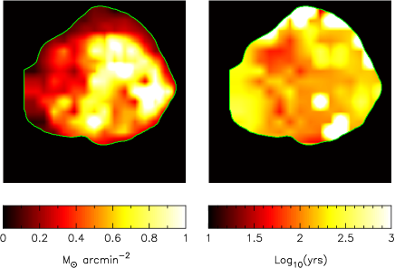
Figure 2: The maps of mass and ionization age of the hot component. The outer contour line indicates the extent of sky coverage with good statistics for spectral fitting.

The larger ages tend to lie around the perimeter while the ages across the central region are relatively constant with a minimum of $\sim 45$ years. Fig. 3 shows the distribution of the shell volume in the temperature ($T_{\rm hot}:T_{\rm cool}$), electron density ($n_{\rm ehot}:n_{\rm ecool}$) and ionisation age ($t_{\rm hot}:t_{\rm cool}$) planes. The electron density and to some extent the temperatures are correlated over the shell volume. However the ionisation ages are not. Note that the ionisation ages are plotted on logarithmic axes. The spread of age is much larger for the cool component than the hot. The differential mass distribution as a function of ionization age for the two components is also shown in Fig. 3. In this distribution we do see a marked difference between the two plasma components. The hot component shows a relatively sharp peak at an ionization age of $\sim 100$ years, whereas the cool component has a broader distribution with a median age of $\sim 80$ years. These profiles indicate that the hot plasma was shock heated over a century ago and the heating process is already complete. The cool plasma, however, has been shocked more recently and the heating process is still ongoing. A small fraction of the mass in both components has an ionization age greater than the true age of the remnant, 320 years, because we have assumed that the densities are constant with time. This is clearly not the case especially when we extrapolate back to the early stages of the remnant expansion.

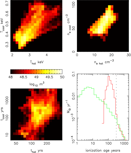
Figure 3: The distribution of shell volume in the temperature, electron density and ionisation age planes. Note that the volume is plotted on a logarithmic scale to reveal the regions with very low volume. The ionisation age scales are logarithmic showing the spread of the volume over several orders of magnitude of the ionisation time. The bottom right panel shows the differential mass distribution of ionization ages. The hot component is shown in red and the cool component is shown in green. The vertical dotted line indicates the age of the remnant (320 years).

4 Projection about the SNR centre

Using the pixel positions with respect to the centre of the remnant on the plane of the sky and the line-of-sight positions provided by the Doppler measurements we can determine the angular distribution of the mass about the centre of the remnant. With $x$ East, $y$ North and $z$ pointing away from the observer we define an axial spherical coordinate system as shown in Fig. 4. The polar axis is labelled $N$ and points towards the receding mass in the North of the remnant. The origin on the equator is in the South East quadrant away from the observer.

Figure 4: The axial spherical coordinate system with respect to the plane of the sky, $x$ East and $y$ North, and the line of sight $z$.

The upper panel of Fig. 5 shows the mass distribution projected in this axial coordinate system in Aitoff projection. It is clear that the entire angular distribution of the emitting mass lies in a band around the remnant with enhancements at the poles in the North and South. (as has been suggested by many observations in the past, see for example Markert et al. 1983). The band of mass is relatively weak when it crosses the equator and there are large solid angle areas around the origin and the anti-centre on the equator where there is very little mass.

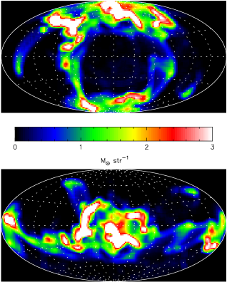
Figure 5: The angular distribution of mass surrounding the centre of Cas A - Aitoff equal area projection. Upper panel in the axial projection and lower panel in the equatorial projection.

The total mass in the Southern hemisphere is $3.3$ $M_{\sun}$ and in the Northern hemisphere is $6.7$ $M_{\sun}$ so the split between the two hemispheres is not equal. Half the mass in the South is contained in $0.63$ steradians, a sky fraction of 0.10 and 90% is contained in $2.0$ steradians (fraction 0.32). Half the mass in the North is contained in $0.75$ steradians, a fraction of 0.12 and 90% is contained in $2.5$ steradians (0.39). The left-hand panel of Fig. 6 shows the mass per steradian as a function of elevation angle in the axial coordinate system. 64% of the mass is contained within a double cone of half angle 45°and the mass density peaks at the poles.

Figure 6: The mass per steradian as a function of elevation angle. Left-hand panel in the axial projection, South -ve elevation, North +ve elevation. Right-hand panel in the equatorial projection.

The mass distribution was reprojected into an equatorial spherical coordinate system in which the equator lies around the band of mass seen in the top panel of Fig. 5. The North pole was shifted to lie at the origin on the equator. The lower panel in Fig. 5 shows this new projection. The right-hand panel of Fig. 6 shows the distribution about the equatorial plane. In this reprojection a fraction of 0.85 of the mass is confined to within $\pm 30$°of the equatorial plane.

The concentration of mass into a small fraction of the available solid angle as shown in Figs. 5 and 6 is consistent with the mean filling factor of $\eta_{\rm hot}=0.31$ (see Table 3) derived from the minumum equilibrium pressure corresponding to a maximum filling factor of $\approx 1.0$. Pressure equilibrium dictates that the filling factor for the cool component is very low, $\eta_{\rm cool}=0.009$. This is consistent with the original rationale for the spectral modelling in which the hot component is assumed to be dominated by surrounding medium heated by the primary shock and potentially enriched by diffuse ejecta, whereas the cool component is assumed to be clumpy ejecta heated by the reverse shock. The differential mass distributions with ionisation age are also consistent with this picture. The bulk of the hot component forms a peak with an ionisaton age in the range 100-180 years while the cool component has a much broader distribution stretching back to $<10$ years, probably indicative of a heating process which is still in progress.

5 The mass and energy budget

The maximum total X-ray emitting mass consistent with the data assuming pressure equilibrium within the remnant volume is $10.0\pm 0.7$ $M_{\sun}$. The maximum total thermal energy visible is $7.0\pm 0.5\times 10^{43}$ J which is a sizeable fraction of the typical total energy released from a SN explosion. The remainder of the energy in the remnant is kinetic. We can estimate this kinetic energy using the expansion velocities discussed above. To estimate the total mass and kinetic energy in the optical FMKs we have assumed a generous hydrogen density of $10^{3}$ cm^-3, (probably reasonably consistent with pressure equilibrium) a total of 120 knots, a knot size of 2″ and a velocity of 5290 km s^-1 (see Reed et al. 1995 and Anderson and Rudnick 1995). Since we have no information about chaotic velocities of optical knots we have assumed these to be zero. Table 4 summarises the resulting mass and energy budget for the remnant.

Table 4: The mass and energy budget for the remnant. $E_{\rm th}$ is the thermal energy and $E_{r}$ is the radial expansion kinetic energy. The hot Ejecta entry (2) are the heavy elements in the hot component, while the hot CSM entry (1) is the fraction of the hot component which is not diffuse ejecta and is presumed to have been circumstellar material at the time of the explosion. The warm ejecta (3) are from the cool X-ray component and the cold ejecta (4) are the optical component. The hot diffuse entry refers to the hot component, which consists of diffuse ejecta and swept-up circumstellar matter. The cool clumpy is the sum of the cool X-ray and optical components also assumed to be ejecta. The total is the sum of all the components.

		$v_{\rm r}$	$M_{\sun}$	$E_{\rm th}$	$E_{\rm r}$	$E_{tot}$
		km s-1		$10^{43}$ J	$10^{43}$ J	$10^{43}$ J
1	hot CSM:	1740	7.9	6.5	2.4	8.9
2	hot ejecta	1740	0.4	0.3	0.1	0.4
3	warm ejecta	1780	1.7	0.2	0.5	0.7
4	cold ejecta	5290	0.1	0.0	0.3	0.3
$\Sigma_{1}^{2}$	hot diffuse	–	8.3	6.8	2.5	9.3
$\Sigma_{3}^{4}$	cool clumpy	–	1.8	0.2	0.8	1.0
$\Sigma_{2}^{4}$	ejecta	–	2.2	0.5	0.9	1.5
$\Sigma_{1}^{4}$	total	–	10.1	7.0	3.3	10.3

The top half of Table is the remnant as we see it now and summing up all the energy components gives an estimate of the total energy released by the explosion, $10.3\times 10^{43}$ J. The cool X-ray component, the optical knots and the heavy elements in the hot X-ray component are almost certainly all remains of the ejecta. The evidence for the X-ray components being emission from ejecta material was put put forward by Willingale et al. (2002). This evidence includes: i) the elemental abundances of Si, S, Ar and Ca are strongly correlated, ii) the elemental abundance values are consistent with enrichment from ejecta material iii) the emitting material is non-uniformally distributed across the remnant. In particular the emission of Fe-K relative to the lighter elements indicate a large degree of non-uniform mixing. The mass labelled hot ejecta in Table 4 are the heavy elements (not H+He) of the hot component. The presence of these elements in the hot component indicates considerable mixing between the swept up interstellar material and the diffuse ejecta. Previous authors, for example Anderson and Rudnick (1995), have identified this component as diffuse ejecta and estimated the mass as $\sim 0.3$ $M_{\sun}$ (Braun 1987), very similar to our estimate of 0.4 $M_{\sun}$. The remaining mass of 7.9 $M_{\sun}$ in the hot component is swept up material labelled hot CSM in Table 4.

Summing up the mass from all the ejecta components indicated in Table 4 and assuming all the energy was kinetic we get the predicted rms ejecta velocity of 6850 km s^-1. The original kinetic energy from the diffuse (now hot) ejecta constitutes the driving mechanism of the primary blast wave. Assuming that all the energy in the hot diffuse medium (i.e. $9.3{\times}10^{43}$ J) was kinetic would require the hot ejecta (0.4 $M_{\sun}$) to have an initial velocity of $\sim 1.5{\times}10^{4}$ km s^-1. We discuss this (quite feasible) velocity further in Sect. 6. The original rms velocity of the clumpy (now cool/cold) ejecta must have been much lower, $\sim 2400$ km s^-1. The velocity of the optical FMFs is 8820 km s^-1 with a deceleration parameter of 0.99 and the velocity of the optical FMKs is 5290 with a deceleration parameter of 0.98 (see tabulation in Willingale et al. 2002 and references ibid) so these ejecta velocity estimate are entirely reasonable. Estimation of the mass and energy in two identifiable parts of the ejecta gives us the first observational glimpse at the ejecta structure function which plays an important role in analytical and numerical modelling of the early stages of the evolution of SNR, see Truelove and McKee (1999). The values in Table 4 are subject to uncertainties which will only be resolved by observations which much higher spectral resolution but overall the mass and energy budget balances reasonably well.

The hot and cool components also contain 0.012 and 0.046 $M_{\sun}$ of iron respectively. It is reasonable to assume that almost all of this iron originated in the ejecta rather than from swept up interstellar medium since most of the material surrounding the star prior to the explosion probably came from the outer hydrogen rich layers of the progentitor (see discussion below). If this is the case $\sim 2.7\%$ of the diffuse and clumpy ejecta mass was iron, now seen as Fe K emission from the hot component and as Fe L emission from the cool component. The hot iron has a significantly larger radial velocity, 2000 km s^-1, than the cool iron, 1580 km s^-1, and is seen at larger radii. It is surprising that iron is seen in the diffuse ejecta especially at large radii in the remnant ahead of the lighter elements since it presumably originated from the core of the progenitor not the outer layers of the star. A great deal of mixing of the layered structure of the progenitor must have occured. This may be because the inner layers were ejected at higher initial velocity than the outer layers and this, in turn, resulted in significant turbulence.

6 Discussion

Just how robust are the values in Table 4? Greatest uncertainty lies in the measurement of the ion temperature and estimation of the volume filling factors. We have set the maximum $\eta_{\rm hot}+\eta_{\rm cool}=1$ while the mean value is $\sim 0.3$ which is entirely consistent with the observed angular coverage shown in Fig. 5. If we abandon pressure equilibrium the $\eta_{\rm cool}$ could increase but the $\eta_{\rm hot}$ would have to decrease and/or the overall filling factor would have to fall. The mean ion temperature is constrained by the measured Doppler broadening of the emission lines. The cool ions could be hotter raising the cool pressure and introducing a pro rata increase in $\eta_{\rm cool}$. This would increase the ejecta mass and decrease the swept up mass but the total mass and energy would remain approximately the same. This, in turn, would decrease the rms velocity of the ejecta which at present is consistent with the measured expansion velocities of the optical knots.

We have not included the magnetic pressure (or energy) in the calculations. The electron pressure in the hot component is $4.3\times 10^{-9}$ Pa, only $\sim 5\%$ of the total pressure and $7.6\times 10^{-9}$ Pa, $\sim 10\%$ of the total pressure in the cool component. A magnetic field of $\sim 2.9$ mG will give the same energy density as the electrons in the hot component but such a large equipartition field is unlikely since the field is being amplified by turbulence and magnetic coupling in the post shock plasma. The mean magnetic field required assuming equipartition with the high energy electrons responsible for the radio synchrotron emission is $\sim 0.5$ mG (Rosenberg 1970, Longair 1994). We conclude that the magnetic energy and relativistic electron energy are only a minor perturbation on the overall energy budget.

Very little of the mass and energy in Table 4 is associated with the faint primary shock which is visible in the Chandra X-ray image (Hughes 2000) and radio images (Anderson & Rudnick 1995). Analysing the Chandra image we find only $\sim 12\%$ of the X-ray flux lies outside the main ring of emission in a region that could be directly associated with the primary shock. It may be that the mass and energy of the primary shock are invisible because the electron temperature has not yet reached the threshold required for X-ray emission. However, we think this is unlikely since the modelling of Laming (2001) indicates that the electrons should reach a temperature of $\sim 3\times 10^{7}$ K only 10 years after being shocked and this translates to an angular shift of 2.5″ on the sky for a shock moving at 4000 km s^-1. It is also possible that slow ejecta lie inside the X-ray emitting shell and this material will remain invisible until it is enveloped by the reverse shock. This could increase the ejecta mass estimate but would have only a minor effect on the total energy. We conclude that hidden mass or energy are unlikely to increase the budget in Table 4 by more than a few percent.

The swept up mass is only seen over about 40% of the total volume of the remnant, Fig. 5. Using an outer radius of 160″ the implied density of the ambient medium within this volume before the explosion was $\sim 13$ cm^-3 which is higher than previous estimates inferred from H II emission (8 cm^-3, Peimbert 1971) deceleration of the radio-emitting material (2 cm^-2, Braun 1987) or the low temperature of the X-ray emitting ring (McKee 1974). This high density CSM provides a link between Cas A and a Wolf-Rayet progenitor that suffered mass-loss forming a nebular shell prior to the supernova explosion. Nebular shells around Wolf-Rayet stars are well observed phenomena. They typically have radii of the order $R\sim 1-4$ pc with shell thickness ${\Delta}R\sim 0.01-0.2$ pc and electron densities $n_{\rm e}$ of a few tens to a few hundreds cm^-3 (Esteban et al. 1993). We suggest some fraction of a nebula shell was initially heated by the primary shock to form the hot CSM entry in Table 4. The hot ejecta have been mixed with this material by turbulence. From the difference between the assumed age of the remnant and the time since the the gas was shocked (see the ionisation age in Table 3), we estimate that the system was in free expansion for the first $\sim$100 years. This time, coupled with the initial velocity ($1.5{\times}10^{4}$ km s^-1) derived in Sect. 5, implies that the material that we now see as hot ejecta had travelled out to a distance of $\sim$1.5 pc (90″) before it hit, and heated, the putative dense nebular shell shed by the progenitor WR star. It then sweeped up about 8 $M_{\sun}$ and is now entering the Sedov phase. These dimensions are consistent with both the observed size of the emitting shell and the typical size of nebular shells observed around WR stars. The cooler ejecta, which have a much lower initial velocity, impacted later and show a broader distribution of ionisation ages centered around a lower average absolute value (see Fig. 3). The emission we see from this component is ablated material formed by “reverse” shock-heating of cool, clumpy ejecta.

The total visible emitting mass calculated above is lower than previous estimates, Fabian et al. (1980) 15 $M_{\sun}$, Vink et al. (1996) 14 $M_{\sun}$. The difference is largely attributable to the lower volume estimates. With better spatial resolution and the benefit of Doppler measurements the estimate of the total fraction of the shell volume which is occupied by the emitting plasma is considerably reduced. The spatially resolved high resolution X-ray spectra provided by XMM-Newton also give us a detailed inventory of the state and composition of the plasma which also reduces the uncertainty in estimating the masses involved. However, the mass loss from the progenitor could still be $\sim 20$ $M_{\sun}$ indicative of a very high loss rate prior to the explosion although only $40\%$ of this material is actually visible.

7 Concluding remarks

We have assumed pressure equilibrium between the hot and cool plasma components to give an estimate of the filling factors within the shell volume. X-ray spectroscopy at higher spectral and spatial resolution could be used to test this assumption. Well resolved emission lines from individual knots would be associated with either the hot or cool component and observation of Doppler broadening of such lines would give us a direct measurement of the ion velocities for individual ion species in the ejecta and swept up material.

Possible supernova core collapse geometries are shown in Fig. 7.

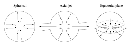
Figure 7: Supernova collapse geometries

The distribution of X-ray emitting mass around Cas A indicates that the original explosion was not symmetric but somewhere between an axial jet and equatorial plane geometry. The confinement to within $\pm 30$°of the equatorial plane as shown in Fig. 6 is rather striking and the other panel in Fig. 6 clearly demonstrates the enhancement of the emission around the poles in the axial coordinate system. It is noteworthy that spherical collapse can be modelled in one dimension, and the axial or equatorial symmetry can be modelled using just two dimensions but the combination of axial and equatorial would require a full three dimensional treatment. It may be that the processes responsible for what we observe will only be revealed by such three dimensional modelling. The apparent asymmetry of the explosion geometry introduces the possiblity of significant shear within the expanding material during or just after the explosion. This may be the root cause of the turbulence and the clumpiness of the mass distribution in the remnant rather than hydrodynamic instabilities in the dense shell formed much later after a significant mass of surrounding material has been swept up.

The total kinetic energy derived for the ejecta is consistent with the canonical value of $10^{44}$ J. However measurements suggest that the ejected mass was rather large and the rms ejection velocity was correspondingly modest. Cas A was most emphatically a mass dominated rather than radiation dominated supernova explosion. This is in stark contrast with, for example, the Crab Nebula in which no significant ejected mass or energy from the original explosion has been identified, see for example Hester et al. (1995). Collimated or jet-induced hypernovae have been suggested as a possible solution to the energy budget problem posed by gamma ray bursts seen from cosmological distances, Wang & Wheeler (1998). However in these cases we are looking for collimation in a radiation dominated explosion. There is no reason to suppose that the degree of mass collimation seen in Cas A is connected with radiation collimation inferred in gamma ray burst events.

- (1) Anderson, M.C., & Rudnick, L., 1995, ApJ, 441, 307
- (2) Aschenbach B., Egger, R. & Trümper, J. 1995, Nature, 373, 587
- (3) Braun, R. 1987, A&A, 171, 233
- (4) Braun, R., Gull, S.F., & Perley, R.A. 1987, Nature, 327, 395
- (5) Esteban, C., Smith L.J., Vílchez, J.M., & Clegg, R.E.S., 1993, A&A, 272, 299
- (6) Fabian, A.C., Willingale R., Pye J.P., Murray S.S., Fabbiano G. 1980, MNRAS, 193, 175
- (7) Hester, J.J., Scowen, P.A., Sankrit, R., et al. 1995, ApJ 448, 240
- (8) Hughes, J.P., Rakowski, C.E., Burrows, D.N., & Slane, P.O. 2000, ApJ, 528, L109
- (9) Laming, J.M. 2001, ApJ, 563, 828
- (10) Longair, M.S. 1994, High Energy Astrophysics, Vol.2, Cambridge Univ. Press
- (11) Markert, T.H., Canizares, C.R., Clark, G.W., & Winkler, P.F., 1983, ApJ, 268, 13
- (12) McKee C.F. 1974, ApJ, 188, 335
- (13) Reed, J.E., Hester, J.J., Fabian, A.C., & Winkler, P.F. 1995, ApJ, 440, 706
- (14) Rosenberg, I., 1970, MNRAS, 151, 109
- (15) Truelove, K.J. and McKee, C.F. 1999, Ap.J.Supp.Ser. 120, 299-326
- (16) Vink, J., Kaastra, J.S., & Bleeker, J.A.M. 1996, A&A, 307, L41
- (17) Wang, L. & Wheeler, J.C., 1998, ApJ, 504, L87
- (18) Willingale R., Bleeker J.A.M., van der Heyden K.J., Kaastra J.S., & Vink J., 2002, A&A 381, 1039-1048