The Spatially-Resolved Mass Function of the Globular Cluster M22

Abstract

HST imaging of M22 has allowed, for the first time, a detailed and uniform mapping of mass segregation in a globular cluster. Luminosity and mass functions from the turnoff down to the mid to lower main sequence are presented for M22 in annular bins from the centre of the cluster out to five core radii. Within the core, a significant enhancement is seen in the proportion of 0.5-0.8 $M_{\sun}$ stars compared with their numbers outside the core. Numerical modelling of the spatial mass spectrum of M22 shows that the observed degree of mass segregation can be accounted for by relaxation processes within the cluster. The global cluster mass function for M22 is flatter than the Salpeter IMF and cannot be represented by a single power law.

1 Introduction

As in many areas of astronomy, the advent of the Hubble Space Telescope has revolutionised the study of globular clusters. Primarily because of crowding, ground-based observations of the central regions of globular clusters are limited to brighter stars, at or above the main sequence turnoff. HST allows access to the study of stellar populations below the turnoff including main sequence stars and white dwarfs.

Main-sequence stars below the turnoff in globular clusters (typically $m<0.8M_{\sun}$) have evolved little from their initial zero-age main-sequence (ZAMS) state. Thus, mass functions derived from globular cluster luminosity functions can be used as indicators of a stellar initial mass function (IMF). Most notably in recent years, several groups have used HST WFPC2 photometry to probe mass and luminosity functions for several globular clusters down to the hydrogen burning limit. For example, Paresce & De Marchi (2000) have documented the turnover in the luminosity function at $\sim 0.3M_{\sun}$ for a sample of twelve Galactic globular clusters. In NGC 6397 King et al. (1998) found that the mass function increases slowly for masses down to 0.1 $M_{\sun}$ and then drops rapidly.

Although individual globular cluster main sequence stars are little evolved from the ZAMS, the main sequence itself has been subject to modification by cluster dynamical effects. These include not only intra-cluster effects such as relaxation due to two-body interactions but also tidal interactions between a globular cluster and its Galactic environment. Relaxation of globular clusters has been studied in detail through dynamical equilibrium models (King, 1966; Gunn & Griffen, 1979) and through direct numerical n-body simulations (Aarseth, 1999). A comprehensive review of globular cluster dynamics is given by Meylan & Heggie (1997). Briefly, two-body interactions tend to transfer kinetic energy outward from the core and produce mass segregation, a depletion of the relative fraction of low mass stars in the central regions relative to their proportions outside the core. Only since the mid-1990’s has this effect been reliably observed in globular cluster cores, for example in 47 Tuc (Paresce, De Marchi & Jedrzejewski, 1995), NGC 6752 (Shara et al., 1995) and NGC 6397 (King, Sosin & Cool, 1995). (Note that the core of a globular cluster is usually parameterised by the core radius, $r_{c}$, defined by King (1962) as the scale factor in his empirical formula for the surface density profile.) The most important external dynamic effect is disk shocking, which tends to strip the lightest stars out of a globular cluster during orbital crossings of the Galactic plane. To best avoid both internal and external dynamical modifications, the stellar luminosity functions in globular clusters should be obtained at radii close to the half-light radius of the cluster (Lee, Fahlman & Richer, 1991; Paresce & De Marchi, 2000).

A further complication in deriving a global IMF is the presence of binary main-sequence stars in a globular cluster. Near-equal-mass binary stars appear on a color-magnitude diagram in a main sequence displaced upwards by 0.75 mag (Elson et al., 1998). In only a few cases, for example NGC 6752 (Rubenstein & Bailyn, 1997), has the photometry been sufficiently precise to resolve this binary main sequence. Normally, the presence of binary stars will contaminate a main-sequence luminosity function, particularly in the core of a cluster where, due to mass segregation effects, the binary fraction is highest. In 47 Tuc, Albrow et al. (2001) found the fraction of binary stars to be around 13% in the innermost 4 $r_{c}$, with some evidence that this fraction was highest ($\sim 20\%$) within 1 $r_{c}$, dropping to $\sim 8\%$ at 2.5 $r_{c}$. Such a dropoff was also noted by Rubenstein & Bailyn (1997) in NGC 6752. For globular clusters showing at least a moderate degree of central concentration, $log(r_{tidal}/r_{c})\gtrsim 1.5$, the half-light radius is generally at least several times $r_{c}$ so luminosity functions derived at the half-light radius should be reasonably free from binary contamination.

In this paper we derive the luminosity and mass functions for M22 (NGC 6656), a globular cluster located about one third of the way between the Sun and the Galactic bulge. Our observations (taken as part of another program) are not particularly deep but cover a large spatial area from the center out to several $r_{c}$. Our focus is thus on determining the degree of mass segregation in the middle to upper main sequence rather than on probing the lowest mass stars. From four fields that we subdivide into concentric annular radial bins, we determine how the luminosity and mass functions change with radius in this cluster. Sections 2 and 3 discuss the data and their reduction. In section 4 and 5 we consider the derivation of the luminosity and mass functions. In section 6 we compare these results with a dynamical model for the cluster.

2 Observations

As part of a program to detect gravitational microlensing events by stars within M22 (Sahu et al., 2001), observations were taken during 22 February to 15 June, 1999, using the WFPC2 camera aboard HST. The images were taken at 43 epochs, with a typical separation of about 3 days. A subset of 9 images were taken with a separation of about 1 day, which were dithered at a sub-pixel level. One additional epoch of observations was taken a year later, on 18 February 2000. At each epoch, images were taken of three fields (hereafter referred to as pointings 1-3) in the central region of M22. Most of the observations were taken in the I (F814W) filter, with every fourth observation in the wide-V (F606W) filter. To optimize the overhead and exposure times during a single orbit, the 3 observed fields were so chosen that they used the same guide stars. This avoided the overheads involved in switching between guide stars during an orbit, but led to slight overlap between different fields. The orientation of the images was kept fixed in all the observations. To facilitate cosmic ray removal, the images were taken in pairs for each filter, each with an integration time of 260 sec. For each observed field, the total exposure time is 17160 sec in the F814W filter and 5200 sec in the F606W filter.

The above observations of the central regions of M22 were supplemented with exposures from the HST archive of a field (hereafter pointing 4) at the approximate half-light radius of the cluster, 3.5’ southeast of the cluster center. These consisted of 4$\times$1200 s exposures in F814W and 2$\times$1100 s + 2$\times$1200 s exposures in F606W. A luminosity function from these datasets was derived by De Marchi & Paresce (1997) and later confirmed by Piotto & Zoccali (1999). We thus have 16 different pointing/CCD combinations listed in Table 1. The four WFPC2 pointings used for this paper are shown in Fig. 1 relative to the cluster center which we take to be at J2000 coordinates (18h36m24.2s,-23$\arcdeg$54’12”) from Harris (1996).

Additionally, the HST archival dataset u27xjd01t was used to establish the luminosity function of the Galactic bulge local to M22. This archive consists of a single (non-CRSPLIT) 2400 s F814W exposure, offset from the center of M22 by approximately 9 arcmin to the southwest.

3 Data Reduction

The data frames were initially put through the standard HST on-the-fly calibration pipeline which involves bias and dark subtraction and flat-field correction. The remaining steps in the photometric reduction process were done using the HSTPHOT 1.0 package (Dolphin, 2000a). Data quality images were used to mask bad pixels and vignetted regions. Pairs of images (CR-SPLITs) taken during a single orbit and with the same dither offset and filter were combined for cosmic ray removal. Sky images were then calculated and hot pixels removed.

PSF-fitting photometry was done using the MULTIPHOT task in HSTPHOT 1.0. This program uses the combined signal from all the images at a given pointing for object detection. We used a detection threshold of 3.0 for the minimum signal-to-noise in the combined images. This threshold was deliberately set lower than what would eventually be used in the selection of stars for further analysis in order to prevent marginally-detected stars from contaminating the measurements of their neighbours.

The artificial star routine in MULTIPHOT generates stars randomly from a 2-dimensional color-magnitude grid specified by the user. We chose a grid such that $17\leq{\rm F606W}\leq 28$, $0\leq{\rm F606W-F814W}\leq 3$. These were placed and solved for one at a time on each set of images so that no additional crowding is introduced. The XY position of each artificial star is chosen randomly, but weighted towards regions with the highest stellar densities in order to best represent the real measurement conditions. A subset of these artificial stars from each frame (between 15,000 and 20,000 per frame) was chosen for comparison with the real stars based on the criterion that their input F606W-F814W color was within 0.1 mag of the main-sequence fiducial line (see section 4).

Charge transfer efficiency corrections were made as described in Dolphin (2000b). Aperture corrections to the PSF photometry were made using 150 - 200 bright and relatively isolated stars on each chip of each image. The aperture corrections were typically less than 0.01 mag but were as high as $\sim$ 0.05 mag for the chips sampling the core of the cluster.

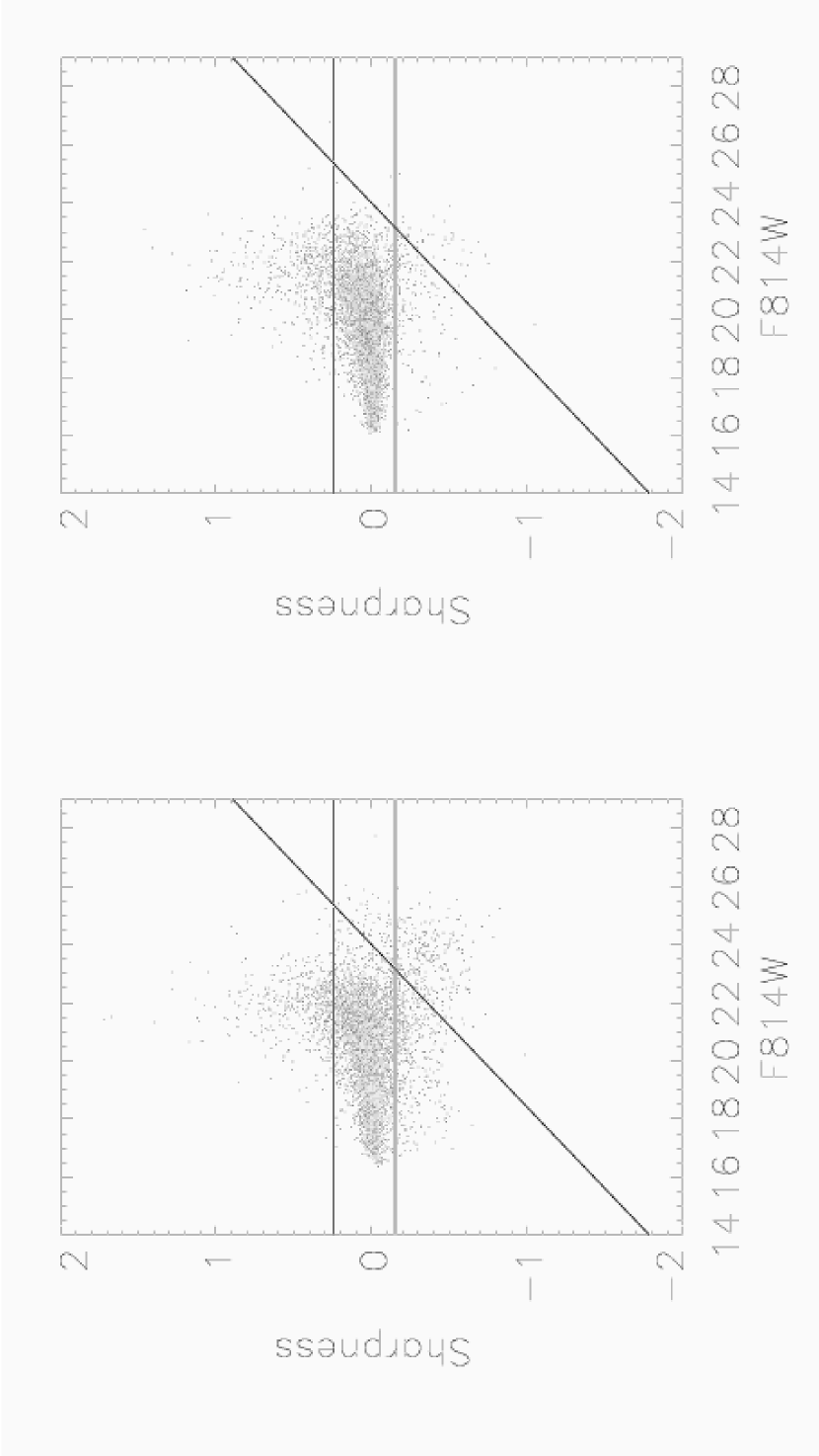
Figure 2: Sharpness criteria for stars in the WF3 chip of pointing 3 between 60” and 120” from the cluster center. The left hand panel shows the observed data and the right hand panel shows the simulated artificial data.

The selection of the final star lists for further analysis was made by imposing a minimum signal-to-noise threshold of 10.0 and making further cuts using sharpness criteria on a chip-by-chip basis. The sharpness reported by HSTPHOT is defined in Dolphin (2000a). A perfectly-fit star has a sharpness of zero, with positive sharpness for stars with a sharper PSF than this, and negative for objects with a broader profile. A completely flat profile has a sharpness value of -1. A typical example of selection by object sharpness is shown in Fig. 2 for the WF3 chip of pointing 3. The sharpness of all the detected objects found between 60” and 120” from the cluster center with S/N $>10$ is plotted against F814W magnitude. (We will use this same sample field for illustrative purposes throughout the paper.) The left-hand panel shows the real data, the right-hand panel the artificial stars. Selection criteria are made with reference to the measured sharpness of the artificial stars. The horizontal cuts are made to reject those stars with poorly-fitting PSFs, the inclined cut is chosen to reject objects found with low sharpness at fainter magnitudes that do not appear in the artificial star set. Some of these faint detections excluded because of their high negative sharpness are image artifacts, mainly lying on diffraction spikes from saturated stars. Others are believed to be blends of faint stars. The adopted sharpness cuts for all field/CCD combinations are given in Table 1.

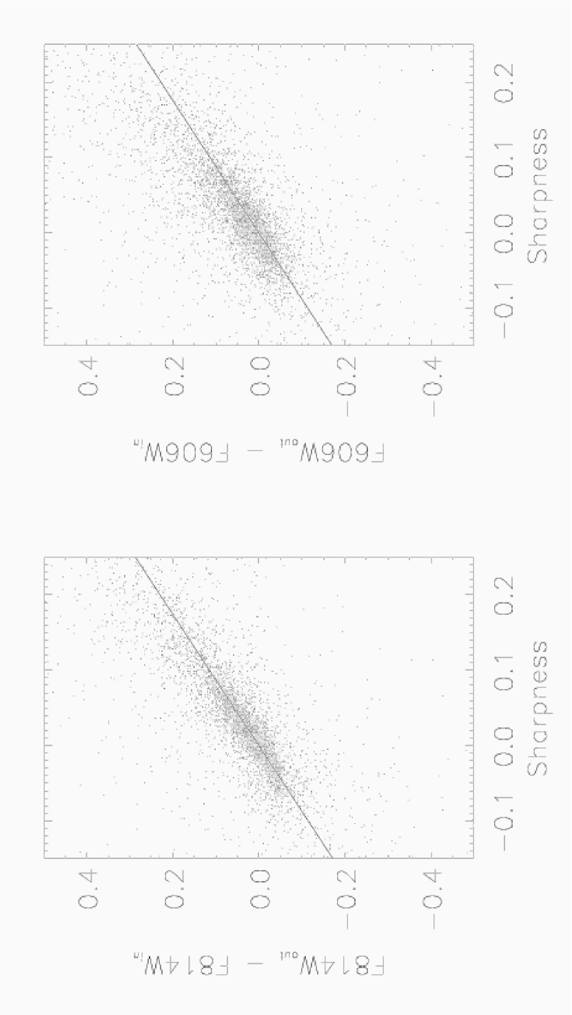
Figure 3: Difference between input and output magnitudes as a function of sharpness for the artificial stars in the sample field.

A further correction to the derived F814W and F606W WFPC2 flight system magnitudes was made to correct a trend with sharpness noticed in the artificial star data. Fig. 3 shows the difference between input and output magnitudes plotted against sharpness for the artificial stars from the same pointing-3 WF3 field as above. This effect is present (with the same slope) for all fields, but as we look farther away from the core the proportion of stars with non-zero sharpness decreases and thus it becomes much less significant. The proportion of stars with non-zero sharpness is also much greater for fainter stars. The origin of the effect can be understood as being due to extreme crowding in the central regions of the cluster. In effect, the background is not the true sky but rather a lumpy morass of undetected stars. The center of a faint, undetected star is more likely to lie in the wings of a brighter (detected) star then on its central pixel, leading it to be measured as being brighter and less sharp. Conversely, a local minimum in the background under a detected star will most likely result in it being measured as being sharper but with a smaller flux. To verify this, we have performed tests in which we have replaced all pixel values below a certain threshold with a constant background value, thus reducing the lumpiness of the background. Artificial stars were then added to the frame in the usual way. The proportion of the artificial stars subject to the effect was found to decrease markedly as this threshold was increased. Since the effect will have influenced all our measurements, the real-star magnitudes were corrected to zero sharpness based on the indicated linear fits to the artificial star data.

4 Luminosity Function

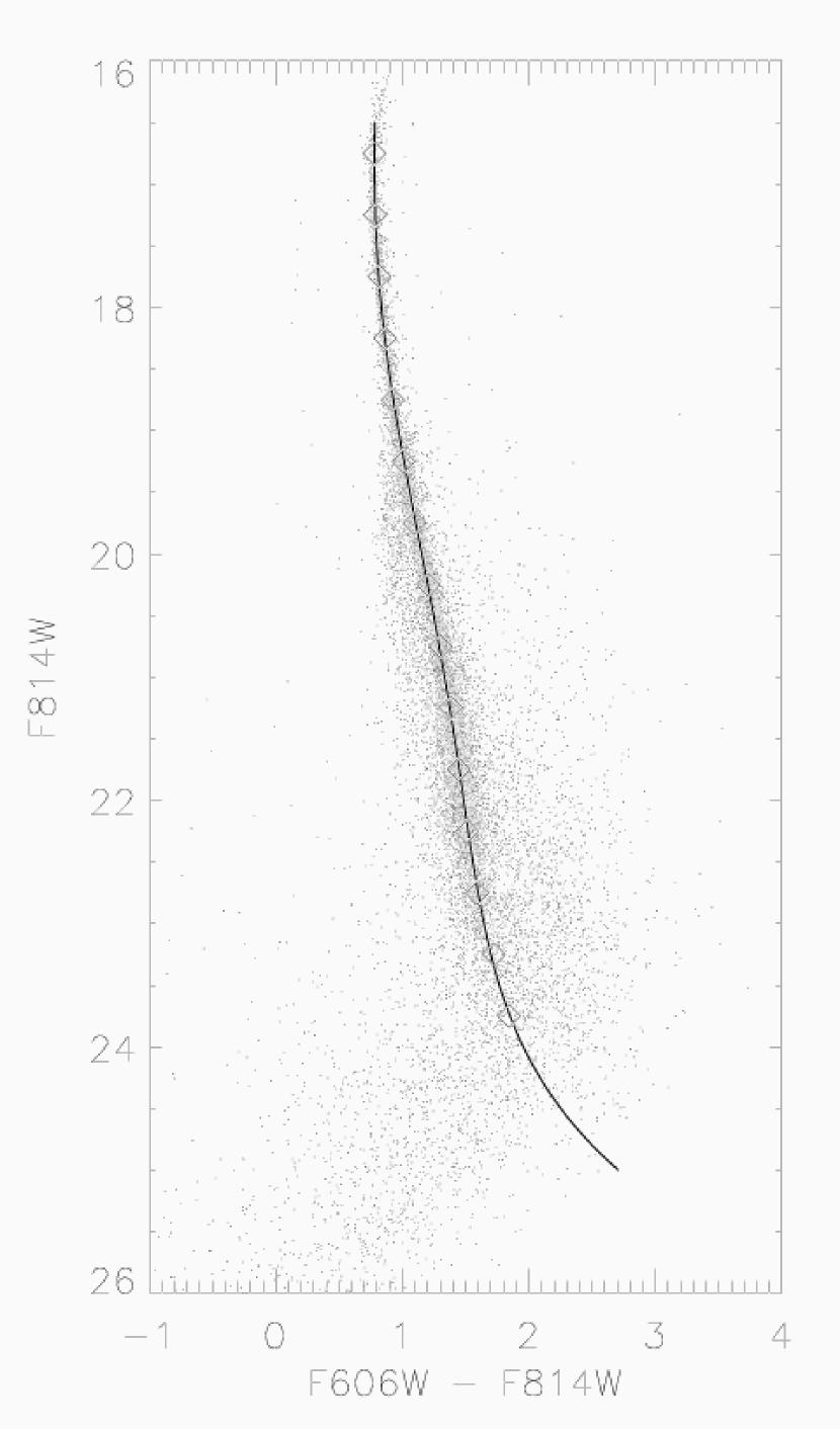
Figure 4: Combined color-magnitude diagram from the 4 PC chips with the main sequence fiducial from a fifth-order polynomial fit.

The combined color-magnitude diagram from the 4 PC chips (one from each pointing) is shown in Fig. 4. All stars with $S/N>4$ and $|sharpness|<0.1$ are included. The S/N threshold was deliberately set to be lower here than what would ultimately be used for our star counts because we wanted to ensure that our main sequence fiducial extended to a fainter limiting magnitude. The adopted main-sequence fiducial is a fifth-order polynomial fit to the median F606W-F814W color in each 0.5-mag F814W band in the range $16.5<{\rm F814W}<24$. A 2.5-$\sigma$ clipping routine was used to reject points with outlying colors in each F814W band before each median color was computed.

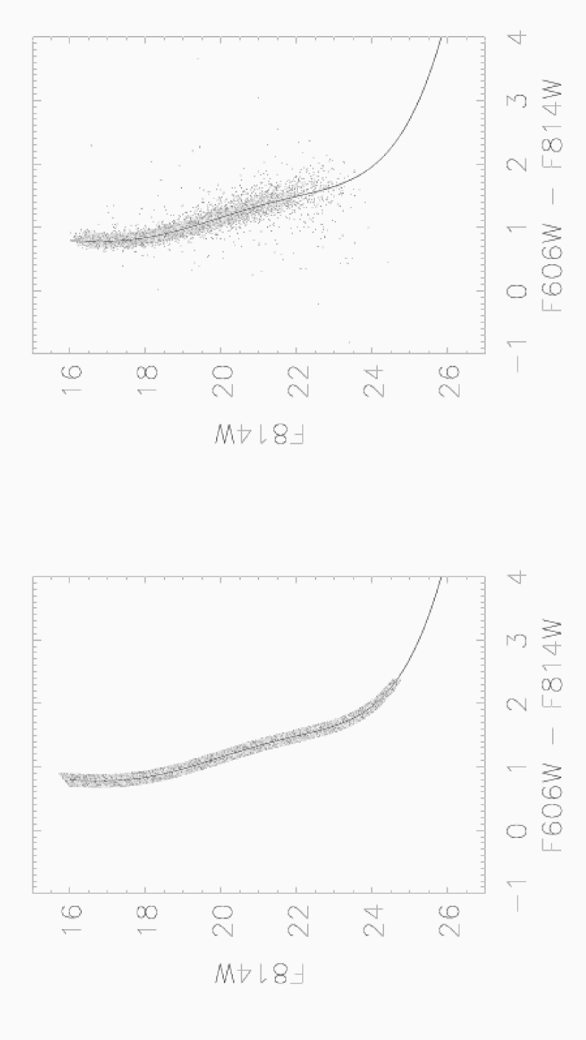
Figure 5: Input (left) and output (right) artificial star color-magnitude diagrams for WF3 pointing-3 field and between 60” and 120” from the cluster center.

In order that our artificial star tests might best represent the actual colors and magnitudes of the measured stars, we selected only those artificial stars whose input magnitudes fell within 0.1 mag in color from the calculated main sequence fiducial. Sample input and output color-magnitude diagrams for the artificial stars in our sample field are shown in Fig. 5.

Since we are interested in determining how the luminosity function of M22 varies as a function of radius from the cluster center, the sets of real and artificial stars for each CCD were divided into concentric annular bins. These annuli were initially chosen at 60” radial intervals extending from the center of the cluster out to 300” as shown in Fig. 1. These 16 CCD fields and 5 radial bins thus give a grid of 80 possible luminosity functions to be calculated. In practice, at most two of these radial bins are well sampled by a given CCD. In order to better sample the core, we repeated our analysis using 20” annuli of which only the innermost five contained sufficient numbers of stars for luminosity functions to be computed with any degree of significance.

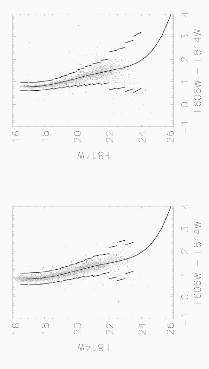
Figure 6: Artificial (left) and real star (right) color-magnitude diagrams for the sample field showing the main sequence fiducial and clipping curves used for statistical adjustment of star counts for field-star contamination.

In Fig. 6 we show the color-magnitude diagram for the sample pointing-3, WF3, 60-120” bin. The left panel shows the real star photometry, the right panel is for the artificial stars. Indicated is the main-sequence fiducial (calculated as described above from the real-star data for all PC fields) and two 2.5-$\sigma$ curves used for statistically correcting the star counts for field-star contamination. Unfortunately the field-star densities of Ratnatunga & Bahcall (1985) do not extend to galactic latitudes as near to the Plane as M22 ($b=-7.55$). The selection curves were calculated from the artificial stars as follows. First, the fiducial main sequence color was subtracted from each point. The resultant $\Delta$(F814W-F606W) values were then subjected to an iterative 2.5-$\sigma$ clipping algorithm, for each 0.5-mag F814W bin and the fiducial main-sequence color added back to the two 2.5-$\sigma$ limits. Thus, in the absence of field-star contamination, 98.75% of main-sequence stars are found between the selection curves. Equivalently, the number of stars outside the selection lines should be 1.26% of the number inside. To estimate field star contamination, we count the number of stars inside and outside the selection lines in each 0.5-mag F814W bin within the color range $-1<{\rm F814W-F606W}<4$. If the outside count is greater than 1.26% of the inner count then we adjust the inner count downwards by the excess, weighted for the differing color-ranges covered. Exactly the same algorithm is applied to the artificial-star data and to the real stars.

The application of the 2.5 $\sigma$ clipping criterion provides us with an upper limit to the luminosity function in that magnitude bins along the main sequence, although clipped to 5 $\sigma$ in color, will also contain background Galactic bulge stars. The bulge color-magnitude diagram (Holtzman et al., 1998) overlaps that of M22 and its luminosity function increases with magnitude.

The luminosity function of the cluster $\phi$ is defined by

$$dN(M)=\phi(M)dM,$$ (1)

where $dN(M)$ is the number of stars per unit area with magnitudes between $M$ and $M+dM$. In each 0.5-mag F814W bin, $\phi_{i}$, is related to the measured star counts, $n_{i}$, by the equation

$$T.{\underline{\phi}}={\underline{n}}$$ (2)

(Drukier et al., 1988). The element $T_{ij}$ of the photometric completion matrix, $T$, represents the probability that a star from magnitude bin $j$ will be measured in magnitude bin $i$. This matrix is constructed from the artificial star counts by comparing each measured F814W magnitude with its input magnitude. For the case of perfect photometry with no “bin jumping”, the matrix is diagonal. In practice, there is a small probability, increasing towards fainter magnitudes, that a given star is scattered up or down in luminosity.

We decided to only measure luminosity functions where the diagonal matrix element was greater than 30%. Experiments showed that constructing the matrix with a limiting magnitude 2 bins below this level was sufficient to assess contamination from fainter stars that have scattered upwards, but not so faint as to cause the matrix to be ill conditioned. The mean photometric completeness in the lowest bin for all our field/annulus combinations was 0.45. One bin above the cutoff, the mean photometric completess was 0.56. In calculating the luminosity function we took into account Poisson errors in the star counts for $n$ and also for the artificial star data in the matrix $T$.

A final scale correction to the derived luminosity functions is made to allow for the spatial area sampled and the 0.5-mag F814W bin size. The individual luminosity functions for the different chip/radius combinations were statistically combined into luminosity functions for each radial bin and the combined luminosity functions from the various fields at different radii from the center of the cluster are given in Tables 2-3 and plotted in Fig. 7.

Also shown in Fig. 7 is a luminosity function we have derived for the Galactic bulge local to M22. For this calculation we used the WFPC2 archival dataset u27xjd01t. This is a single, non-CRSPLIT, 2400 s F814W exposure of a field offset from the center of M22 by approximately 9 arcmin. The four WFPC2 CCD frames from this exposure were processed in the same way as the M22 observations. Artificial star tests were again used to correct the derived luminosity functions for photometric completeness and the corrected luminosity functions for the four chips were statistically combined. The photometric completeness for all chips was around 75% at F814W = 22 and 50% at F814W = 24.

Since the derived bulge luminosity function is approximately linear over $19<{\rm F814W}<23$ we have made a weighted linear fit to the bulge luminosity function in this region, $\log N=0.197{\rm F814W}-1.72$. Comparison with Fig. 5 of Holtzman et al. (1998) shows that the Baade’s window luminosity function is also linear in this region (assuming the same distance and extinction) and has a similar slope. We have corrected our M22 luminosity functions for background bulge contamination by subtracting the indicated linear fit extrapolated to brighter magnitudes. Again referring to Fig. 5 of Holtzman et al. (1998), the Baade’s window luminosity function drops more rapidly for magnitudes brighter than $M_{I}=3.25$ (F814W = 18.5) suggesting we may have over-corrected the brighter magnitudes. However, this over-correction is at most 0.05 in the log luminosity function. Our resulting corrected luminosity functions for M22 are given in Tables 4-5 and shown in Fig. 8.

5 Mass function

To transform the luminosity functions into mass functions we use the 10-Gyr evolutionary models of Baraffe et al. (1997) for metal-poor low-mass stars. These models have been shown to be a good fit to the lower main sequences of globular clusters observed by HST and the authors have made available tables of mass vs luminosity in the WFPC2 flight system filter set. We follow Baraffe et al. (1997) and calculate [M/H] following the prescription of Ryan & Norris (1991) for halo subdwarfs. For the metallicity range of interest, [M/H] $\approx$ [Fe/H] + 0.35. Harris (1996) lists [Fe/H] = $-1.64$ for M22 while Caretta & Gratton (1997) found [Fe/H] = $-1.48$ $\pm$ 0.03. In Fig. 9 we thus compare the main-sequence fiducial of M22 with that predicted by the models for [M/H] = $-1.3$ and [M/H] = $-1.0$. We have transformed the model points to the observational plane using $(m-M)_{V}=13.60$ and $E(B-V)=0.34$ (again from Harris (1996)) and taken the relative extinction coefficients for the WFPC2 filters from Schlegel et al. (1998). The colors and luminosities for both models provide a remarkable match to our photometric main sequence fiducial. We adopt the relation for [M/H] = $-1.0$ as the match is slightly better to both the photometry and the (presumably more accurate) Caretta & Gratton metallicity.

The mass function $\zeta(m)$, defined by

$$dN(m)=\zeta(m)dm$$ (3)

where $dN(m)$ is the number of stars per unit area with masses between $m$ and $m+dm$, is related to the luminosity function $\phi({\rm F814W})$ by

$$\zeta(m)dm=\phi({\rm F814W})d{\rm F814W}.$$ (4)

The mass-luminosity relation from the theoretical [M/H] = -1.0 isochrone was thus used to assign a mass range to each F814W bin. The derivative of the relation at the center of each bin was used to translate the luminosity functions to the mass functions shown in Fig. 10 and listed in Tables 6-7.

The mass functions for the annular bins can be characterised by examining three regions, $\log m\lesssim-0.6$, $-0.6\lesssim\log m\lesssim-0.3$ and $\log m\gtrsim-0.3$. For $\log m\lesssim-0.6$, the mass functions interior to a 180” radius rise towards lower masses with an approximately constant power law index $\alpha\approx 1.0$ to 1.3, where $\zeta(m)\propto m^{-\alpha}$. Our data do not extend to faint enough magnitudes to see any turnover in these mass functions. Between $\log m\approx-0.6$ and $\log m\approx-0.3$ the mass functions are flat ($\alpha\approx 0$). Clear evidence of mass segregation is seen for $\log m\approx-0.3$. Outside of approximately $r_{c}$ (60” - 85”), the mass function decreases with increasing mass ($\alpha\approx 1.2$). Within the core and towards the center, there is an increasing tendancy for the mass function to flatten and then rise towards higher masses, as illustrated in the mass functions for 20” annular bins.

6 Simulation of Dynamical Structure

Having derived the spatially resolved mass function for NGC 6656, we next address the issue as to whether the degree of mass segregation can be accounted for by the theory of relaxation. To study the dynamical properties of the cluster, we have employed the multi-mass Michie–King models originally developed by Meylan (1987, 1988) and later suitably modified by Pulone, De Marchi & Paresce (1999) and De Marchi, Paresce & Pulone (2000) for the general case of clusters with a set of radially varying luminosity functions. Each model run is characterised by a mass function (MF) in the form of an exponential $dN/d\log m\propto m^{-x}$, with a variable exponent $x$ (note that $\alpha=1+x$), and by four structural parameters describing, respectively, the scale radius ($r_{\rm c}$), the scale velocity ($v_{\rm s}$), the central value of the dimensionless gravitational potential ($W_{\rm o}$) and the anisotropy radius ($r_{\rm a}$). From the parameter space defined in this way, we have selected those models that simultaneously fit both the observed surface brightness (SBP) and velocity dispersion (VDP) profiles of the cluster as measured, respectively, by Trager, King & Djorgovski (1995) and Peterson & Cudworth (1994). The fit to the SBP and VDP, however, can only constrain $r_{\rm c}$, $v_{\rm s}$, $W_{\rm o}$, and $r_{\rm a}$ while still allowing the MF to take on a variety of shapes. To break this degeneracy, we further impose the condition that the model MF agree with the observed LF.

Since Michie–King modeling only provides a “snapshot” of the current dynamical state of the cluster, one finds it useful to define the global mass function (GMF), the mass distribution of all cluster stars at present, as the MF that the cluster would have simply as a result of stellar evolution (that is, ignoring any local modifications induced by internal dynamics and/or the interaction with the Galactic tidal field). Clearly, in this case the IMF and GMF of main sequence (un-evolved) stars is the same. For practical purposes, the GMF has been divided into sixteen different mass classes, covering main sequence stars, white dwarfs, and heavy remnants, precisely as described in Pulone, De Marchi & Paresce (1999).

Our parametric modelling approach assumes energy equipartition amongst stars of different masses. Thus, we have run a large number of trials to see whether we could find a set of parameters for the GMF (i.e. a suitable GMF “shape”) such that the local MFs produced by mass segregation would locally fit the observations. Our exercise confirms what we had already implicitly shown in Fig. 10 and described above: as long as a single value of the exponent $x$ is used for the GMF over the mass range $0.2-0.8$ M_⊙, none of the predicted MF can be fitted to our data. In fact, a change of slope is needed at $m\simeq 0.4$ M_⊙ so that both the flat and rising portions of the local MF can be reproduced. If we then allow the MF to take on more than one slope, the GMF that best fits the observations is one with $x=0.2$ ($\alpha=1.2$) for stars in the range $0.4-0.8$ M_⊙ and $x=-0.5$ ($\alpha=0.5$) at smaller masses.

Although stars more massive than $\sim 0.8$ M_⊙ have evolved and are no longer visible, the shape of the IMF in this mass range has strong implications as to the fraction of heavy remnants in the cluster and, as such, on the central velocity dispersion. We find that a value of $x=0.9$ ($\alpha=1.9$) for stars in the range $100-0.8$ M_⊙ gives the best fit to the data and to the cluster’s structural parameters as given in the literature. The latter, along with those of our best fitting model, are presented in Table 8. The agreement is excellent, apart from a small difference in the value of the core radius. We note here that global cluster MF is shallower than Salpeter’s IMF, which would have $x=1.35$. The total implied cluster mass is $2.7\times 10^{5}$ M_⊙ and the mass-to-light ratio is on average $m/L=1.6$, with $m/L\simeq 2$ in the core. These are all very typical values for a cluster of this type and confirm that the observed degree of mass segregation is indeed what would be expected from dynamical relaxation.

7 Summary

Extensive HST imaging of M22 has been used to determine the luminosity function for this globular cluster at a number of different radii from the cluster center. Using the Baraffe et al. (1997) stellar isochrones, we have transformed these luminosity functions into mass functions. The proportion of higher-mass stars was found to be significantly enhanced within one core radius of the center of the cluster compared to regions outside the core. This is the first time that such a detailed mapping of mass segregation from the mid main sequence to the turnoff has been performed for a globular cluster.

Numerical simulation of the radial mass spectrum of M22 using multi-mass King-Michie models has shown that the degree of mass segregation found is well predicted by the standard theory of cluster relaxation.

Figure 1: Area coverage of the 4 WFPC2 pointings relative to 60” annular bins around the cluster center.

Figure 7: Luminosity function for concentric annular bins from the center of the cluster with the uppermost curve in each panel being for the central circular bin. The lowest curve in each panel (dotted line) is the bulge luminosity function measured from an archival exposure offset from M22. A linear fit to the bulge luminosity function is indicated with a dashed line. The left panel is for annular bins of 60” radial increment and the right hand panel is for the innermost five annuli with a 20” radial increment.

Figure 8: Luminosity functions from Fig. 7 that have had the background Galactic bulge luminosity function subtracted.

Figure 9: Observed main-sequence fiducial (solid line) with models of Baraffe et al. (1997) for [M/H] = -1.3 (numbered to left) and [M/H] = -1.0 (numbered to right) with masses indicated. The model points have been transformed to the observational plane assuming $(m-M)_{V}=13.6$ and $E(B-V)=0.34$ from Harris (1996) and the extinction coefficients of Schlegel et al. (1998).

Figure 10: Mass function for concentric annular bins from the center of the cluster with the uppermost curve in each panel being for the central circular bin. The left panel is for annular bins of 60” radial increment and the right hand panel is for the innermost five annulli with a 20” radial increment.

Figure 11: Observed MFs (boxes) and the MFs predicted by the model (solid lines) at the radial distances 14”, 32”, 51”, 95”, 153” and 212”. These distances are at the geometric mean of each measured annulus. Error bars are not plotted as they are comparable or (usually) smaller than the size of the symbols.

Table 1: CCD fields and sharpness cut criteria

Field Name	Pointing	CCD	Sharpness cut criteria
			Min	Max	Slope	Zero point
1	1	PC1	-0.15	0.20	2.5	-4.29
2	1	WF2	-0.15	0.25	2.5	-4.29
3	1	WF3	-0.15	0.25	2.5	-4.29
4	1	WF4	-0.15	0.25	2.5	-4.29
5	2	PC1	-0.15	0.20	2.5	-4.29
6	2	WF2	-0.15	0.25	2.5	-4.29
7	2	WF3	-0.15	0.25	2.5	-4.29
8	2	WF4	-0.15	0.25	2.5	-4.29
9	3	PC1	-0.15	0.20	2.5	-4.29
10	3	WF2	-0.15	0.25	2.5	-4.29
11	3	WF3	-0.15	0.25	2.5	-4.29
12	3	WF4	-0.15	0.25	2.5	-4.29
13	4	PC1	-0.15	0.20	2.5	-4.46
14	4	WF2	-0.15	0.25	2.5	-4.46
15	4	WF3	-0.15	0.25	2.5	-4.46
16	4	WF4	-0.15	0.25	2.5	-4.46

Table 2: Combined Luminosity functions for 60” annular bins

Radius	0–60		60–120		120–180		180–240		240–300
F814W	$\phi$	$\sigma_{\phi}$	$\phi$	$\sigma_{\phi}$	$\phi$	$\sigma_{\phi}$	$\phi$	$\sigma_{\phi}$	$\phi$	$\sigma_{\phi}$
17.0-17.5	1103	27	506	16	317	66
17.5-18.0	1416	27	677	16	395	44
18.0-18.5	1618	26	849	15	487	43
18.5-19.0	1739	29	975	15	564	42
19.0-19.5	1519	29	937	15	591	42
19.5-20.0	1504	33	963	14	628	22	532	45	351	68
20.0-20.5	1643	42	1054	15	701	21	562	34	410	64
20.5-21.0	1770	129	1214	17	847	22	684	30	441	59
21.0-21.5	1991	272	1514	21	1166	25	916	32	572	59
21.5-22.0	2731	344	1769	45	1222	29	1075	35	666	60
22.0-22.5	2390	362	1825	170	1174	50	881	42	671	67
22.5-23.0			1838	415	1244	201	856	49	732	83
23.0-23.5							725	178	577	84
23.5-24.0							818	230

Table 3: Combined Luminosity functions for 20” annular bins

Radius	0–20		20–40		40–60		60–80		80–100
F814W	$\phi$	$\sigma_{\phi}$	$\phi$	$\sigma_{\phi}$	$\phi$	$\sigma_{\phi}$	$\phi$	$\sigma_{\phi}$	$\phi$	$\sigma_{\phi}$
17.0-17.5	1556	120	1171	45	941	40	610	32	473	49
17.5-18.0	1911	113	1543	46	1193	40	797	30	644	39
18.0-18.5	2016	113	1915	46	1363	39	1038	30	823	38
18.5-19.0	2515	145	1840	50	1506	40	1164	30	890	37
19.0-19.5	1961	145	1621	52	1316	38	1102	30	931	36
19.5-20.0	1777	184	1544	60	1406	44	1131	30	915	36
20.0-20.5			1623	100	1554	52	1104	32	1068	37
20.5-21.0			1319	396	1677	111	1410	43	1186	44
21.0-21.5					1987	309	1830	80	1447	65
21.5-22.0					2522	384	2216	169	1627	159
22.0-22.5					2027	391	2063	175
22.5-23.0							2067	395

Table 4: Combined Luminosity functions for 60” annular bins after subtraction of the background Galactic bulge luminosity function.

Radius	0–60		60–120		120–180		180–240		240–300
F814W	$\phi$	$\sigma_{\phi}$	$\phi$	$\sigma_{\phi}$	$\phi$	$\sigma_{\phi}$	$\phi$	$\sigma_{\phi}$	$\phi$	$\sigma_{\phi}$
17.0-17.5	1055	27	458	16	269	66
17.5-18.0	1356	27	617	16	335	44
18.0-18.5	1543	26	774	15	412	43
18.5-19.0	1645	29	881	15	470	42
19.0-19.5	1401	29	819	15	472	42
19.5-20.0	1356	33	814	14	480	22	384	45	203	68
20.0-20.5	1456	42	868	15	515	21	375	34	224	64
20.5-21.0	1537	129	981	17	613	22	451	30	207	59
21.0-21.5	1697	272	1221	21	873	25	623	32	278	59
21.5-22.0	2364	344	1402	45	854	29	707	35	298	60
22.0-22.5	1928	362	1364	170	712	50	419	42	210	67
22.5-23.0			1259	415	665	201	276	49	153	83

Table 5: Combined Luminosity functions for 20” annular bins after subtraction of the background Galactic bulge luminosity function.

Radius	0–20		20–40		40–60		60–80		80–100
F814W	$\phi$	$\sigma_{\phi}$	$\phi$	$\sigma_{\phi}$	$\phi$	$\sigma_{\phi}$	$\phi$	$\sigma_{\phi}$	$\phi$	$\sigma_{\phi}$
17.0-17.5	1509	120	1123	45	893	40	563	32	425	49
17.5-18.0	1852	113	1483	46	1133	40	737	30	584	39
18.0-18.5	1940	113	1839	46	1288	39	963	30	748	38
18.5-19.0	2421	145	1745	50	1412	40	1070	30	795	37
19.0-19.5	1843	145	1503	52	1198	38	984	30	812	36
19.5-20.0	1629	184	1396	60	1257	44	982	30	767	36
20.0-20.5			1436	100	1367	52	918	32	882	37
20.5-21.0			1086	396	1444	111	1176	43	953	44
21.0-21.5					1694	309	1537	80	1154	65
21.5-22.0					2154	384	1849	169	1259	159
22.0-22.5					1565	391	1601	175
22.5-23.0							1488	395

Table 6: Mass functions for 60” annular bins

Radius	60		120		180		240		300
Mass	$\zeta$	$\sigma_{\zeta}$	$\zeta$	$\sigma_{\zeta}$	$\zeta$	$\sigma_{\zeta}$	$\zeta$	$\sigma_{\zeta}$	$\zeta$	$\sigma_{\zeta}$
0.772-0.811	13563	347	5895	208	3461	853
0.724-0.772	14407	286	6559	167	3556	467
0.670-0.724	14045	238	7042	139	3749	388
0.617-0.670	15463	274	8278	141	4414	392
0.567-0.617	14128	294	8261	149	4763	419
0.519-0.567	14008	342	8410	149	4954	231	3967	469	2094	705
0.467-0.519	14140	405	8424	146	4998	206	3645	328	2176	626
0.408-0.467	13187	1109	8416	147	5264	186	3868	255	1780	505
0.336-0.408	11895	1909	8556	150	6120	175	4365	222	1951	412
0.264-0.336	16283	2371	9655	312	5882	200	4873	238	2052	416
0.214-0.264	19413	3649	13728	1714	7172	503	4221	422	2114	677
0.176-0.214			16511	5445	8713	2636	3625	648	2010	1086

Table 7: Mass functions for 20” annular bins

Radius	20		40		60		80		100
Mass	$\zeta$	$\sigma_{\zeta}$	$\zeta$	$\sigma_{\zeta}$	$\zeta$	$\sigma_{\zeta}$	$\zeta$	$\sigma_{\zeta}$	$\zeta$	$\sigma_{\zeta}$
0.772-0.811	19398	1539	14442	584	11487	514	7235	406	5462	624
0.724-0.772	19674	1196	15758	488	12037	420	7835	322	6202	412
0.670-0.724	17661	1025	16740	419	11725	352	8767	275	6808	348
0.617-0.670	22756	1363	16406	469	13270	379	10055	285	7476	351
0.567-0.617	18588	1465	15158	526	12080	387	9925	302	8192	367
0.519-0.567	16824	1903	14420	620	12987	456	10146	306	7922	367
0.467-0.519			13946	973	13277	509	8914	310	8563	362
0.408-0.467					12388	950	10091	368	8174	373
0.336-0.408					11872	2168	10771	563	8084	453
0.264-0.336					14840	2646	12735	1161	8673	1092
0.214-0.264					15758	3940	16123	1761
0.176-0.214							19507	5180

Table 8: Parameters for the King-Michie model. References are (1) Harris (1996) (2) Peterson & Cudworth (1994)

Parameter	Simulation value	Literature value	Reference
Core radius	60”	85”	1
Concentration	1.3	1.3	1
Tidal radius	29’	29’	1
Velocity dispersion	7 km s-1	7 km s-1	2

References

- Aarseth (1999) Aarseth, S.J., 1999, PASP, 111, 1333
- Albrow et al. (2001) Albrow, M.D., Gilliland, R.L., Brown, T.M., Edmonds, P.D., Guhathakurta P., Sarajedini A., 2001, ApJ, 559, 1060
- Baraffe et al. (1997) Baraffe, I., Chabrier, G., Allard, F., Hauschildt, P.H., 1997, A&A, 327, 1054
- Caretta & Gratton (1997) Caretta, E., Gratton, R.G., 1997, A&AS, 121, 95
- De Marchi & Paresce (1997) De Marchi, G., Paresce, F., 1997, ApJ, 476, L19
- De Marchi, Paresce & Pulone (2000) De Marchi, G., Paresce, F., Pulone, L., 2000, ApJ, 530, 342
- Dolphin (2000a) Dolphin, A.E., 2000, PASP, 112, 1383
- Dolphin (2000b) Dolphin, A.E., 2000, PASP, 112, 1397
- Drukier et al. (1988) Drukier, G.A., Fahlman, G.G., Richer, H.B., Vandenberg, D.A., 1988, AJ, 95, 1415
- Elson et al. (1998) Elson, R.A.W., Sigurdsson, S., Davies, M., Hurley, J., Gilmore, G., 1998, MNRAS, 300, 857
- Gunn & Griffen (1979) Gunn, J.E., Griffen, R.F., 1979, AJ, 84, 752
- Harris (1996) Harris, W.E., 1996, AJ, 112, 1487
- Holtzman et al. (1998) Holtzman, J.A., Watson, A.M., Baum, W.A., Grillmair, C.J., Groth, E.J., Light, R.M., Lynds, R., O’Neil, E.J., 1998, AJ, 115, 1946
- King (1962) King, I.R., 1962, AJ, 67, 471
- King (1966) King, I.R., 1966, AJ, 71, 64
- King, Sosin & Cool (1995) King, I.R., Sosin, C., Cool, A.M., 1995, ApJ, 452, L33
- King et al. (1998) King, I.R., Anderson, J., Cool, A.M., Piotto, G., 1998, ApJ, 492, L37
- Lee, Fahlman & Richer (1991) Lee, H.M., Fahlman, G.G., Richer, H.B., 1991, ApJ, 366, 455
- Meylan (1987) Meylan, G., 1987, A&A, 184, 144
- Meylan (1988) Meylan, G., 1988, A&A, 191, 215
- Meylan & Heggie (1997) Meylan, G., & Heggie, D.C., 1997, A&A Rev., 8, 1
- Paresce, De Marchi & Jedrzejewski (1995) Paresce, F., De Marchi, G., Jedrzejewski, R., 1995, ApJ, 442, L57
- Paresce & De Marchi (2000) Paresce, F., De Marchi, G., 2000, ApJ, 534, L870
- Peterson & Cudworth (1994) Peterson, R.C., Cudworth, K.M., 1994, ApJ, 420, 612
- Piotto & Zoccali (1999) Piotto, G., Zoccali, M., 1999, A&A, 345, 485
- Pulone, De Marchi & Paresce (1999) Pulone, L., De Marchi, G., Paresce, F., 1999, A&A, 342, 440
- Ratnatunga & Bahcall (1985) Ratnatunga, K.U., Bahcall, J.N., 1985, ApJ, 59, 63
- Rubenstein & Bailyn (1997) Rubenstein, E.P., Bailyn, C.D., 1997, ApJ, 474, 701
- Ryan & Norris (1991) Ryan, S.G., Norris, J.J., 1991, AJ, 101, 1865
- Sahu et al. (2001) Sahu, K.C., Casertano, S., Livio, M., Gilliland, R.L., Panagia, N., Albrow, M.D., Potter, M., 2001, Nature, 411, 1022
- Shara et al. (1995) Shara, M.M., Drissen, L., Bergeron, L.E., Paresce, F., 1995, ApJ, 441, 617
- Schlegel et al. (1998) Schlegel, D.J., Finkbeiner, D.P., Davis, M., 1998, ApJ, 500, 525
- Trager, King & Djorgovski (1995) Trager, S.C., King, I.R., Djorgovski, S., 1995, AJ, 109, 218