Photoelectric Heating and [C II] Cooling of High Galactic Latitude Translucent Clouds

Abstract

The (${}^{2}{\rm P}_{\rm\scriptscriptstyle 3/2}\rightarrow{{}^{2}\rm P}_{\rm\scriptscriptstyle 1/2}$) transition of singly–ionized carbon, [C II], is the primary coolant of diffuse interstellar gas. We describe observations of [C II] emission towards nine high Galactic latitude translucent molecular clouds, made with the long wavelength spectrometer on board the Infrared Space Observatory. To understand the role of dust grains in processing the interstellar radiation field (ISRF) and heating the gas, we compare the [C II] integrated intensity with the far-infrared (FIR) integrated surface brightness for the 101 sampled lines of sight. We find that [C II] is linearly correlated with FIR, and the average ratio is equal to that measured with the COBE satellite for all high-latitude Milky Way gas. There is a significant decrease that was not detected with COBE in [C II] emissivity at high values of FIR. Our sample splits naturally into two populations depending on the 60µm/100µm surface brightness ratio, or color: “warm” positions with $60/100>0.16$, and “cold” positions with $60/100<0.16$. A transition from sources with warm to those with cold 60/100 colors coincides approximately with the transition from constant to decreasing [C II] emissivity. We model the [C II] and far–infrared emission under conditions of thermal equilibrium, using the simplifying assumptions that, in all regions heated by the ISRF, the most important source of gas heating is the photoelectric effect on grains and the most important source of gas cooling is [C II] emission. The model matches the data well, provided the ISRF incident flux is $\chi_{0}\approx 1.6$ (in units of the nominal value near the Sun), and the photoelectric heating efficiency is $\epsilon\approx 4.3\%$. There are no statistically significant differences in the derived values of $\chi_{0}$ and $\epsilon$ for warm and cold sources. The observed variations in the [C II] emissivity and the 60/100 colors can be understood entirely in terms of the attenuation and softening of the ISRF by translucent clouds, not changes in dust properties.

1 Introduction

Diffuse interstellar gas clouds are heated by the absorption of starlight and cooled by the emission of spectral line radiation at far–infrared (FIR) and submillimeter wavelengths. Energy can be transferred from the interstellar radiation field (ISRF) to the gas by the photoelectric effect on dust grains (Watson, 1972; de Jong, 1977; Draine, 1978; Bakes & Tielens, 1994), whereby far ultraviolet (FUV) (6 eV $<h\nu<$ 13.6 eV) photons ionize grains and the ejected electrons heat the gas through collisions. In diffuse H I regions of low kinetic temperature (${{\rm T_{\rm k}}}\sim 50-200\,{\rm K}$), the “cold neutral medium” (CNM), this process is thought to be the dominant gas heating mechanism (see Wolfire et al., 1995).

The most abundant form of carbon gas in the CNM is the singly-ionized carbon atom, C II, because the first ionization potential of carbon is 11.3 eV and the CNM is permeated by FUV photons. The 158µm (${}^{2}{\rm P}_{\rm\scriptscriptstyle 3/2}\rightarrow{{}^{2}\rm P}_{\rm\scriptscriptstyle 1/2}$) emission line transition of [C II] should be the primary coolant of the CNM (Wolfire et al., 1995). There are two main reasons for this. First, the C II ion is relatively easy to excite by collisions given average CNM temperatures ($T\sim 80\,{\rm K}$;Kulkarni & Heiles 1987). After the hyperfine states of hydrogen, the ${}^{2}P_{3/2}$ fine structure state of C II is the first excited state ($h\nu/k=91\,{\rm K}$) of all gas-phase CNM constituents (the next state is the ${}^{3}P_{1}$ level of the O I atom, which is 228$\,{\rm K}$ above ground). Second, once excited, the energy loss rate, given by the product $h\nu\,A_{ul}\times{{{\rm N}_{\rm\scriptscriptstyle CII}}}[^{2}P_{3/2}]$, is much higher for C II than for other CNM species. Here $A_{ul}$ is the Einstein spontaneous emission coefficient for the ${}^{2}{\rm P}_{\rm\scriptscriptstyle 3/2}\rightarrow{{}^{2}\rm P}_{\rm\scriptscriptstyle 1/2}$ transition and ${{{\rm N}_{\rm\scriptscriptstyle CII}}}[^{2}P_{3/2}]$ is the column density of C II in the excited state .

Since the FUV radiation field that ionizes dust grains (and thus heats the gas) can also heat the grains, one expects a connection between the [C II] 158µm line emission from photoelectron-heated gas and the far-infrared (FIR) emission from FUV-heated dust grains. Large-scale surveys of the Galaxy indeed reveal a link between the C II and FIR emission properties of the CNM. An unbiased survey of spectral line and continuum emission in the Milky Way was conducted with two instruments on board the Cosmic Background Explorer (COBE) satellite: the Far Infrared Absolute Spectrometer (FIRAS) and the Diffuse Infrared Background Experiment (DIRBE). The [C II] emission was observed with FIRAS to be closely correlated with H I emission at high Galactic latitudes, with an average C II cooling rate of $(2.65\pm 0.15)\times 10^{-26}\,$erg s${}^{-1}\,$(H atom)^-1 (Bennett et al., 1994). Both DIRBE and FIRAS maps of the dust continuum show that the dust opacity and FIR surface brightness are also correlated with H I column density at high latitude (Boulanger et al., 1996).

So on the large scale (FIRAS has an angular resolution of 7°, DIRBE of 40′), CNM H I gas has constant FIR and [C II] emissivity. It is therefore likely that the processing of FUV radiation by dust grains (1) to produce FIR dust emission and (2) to heat the gas—resulting in [C II] emission—occurs in similar ways throughout the cold interstellar medium. It is difficult to test this idea directly using the COBE data, mainly because of inadequate resolution. The emission from gas with vastly different physical conditions, for example molecular and atomic gas, might be combined together in a single FIRAS or DIRBE measurement, making it impossible to understand the physical mechanisms responsible for the observed emission.

High resolution observations of the [C II] and FIR emission from translucent molecular clouds can be used to test the limits of models for gas heating by the ISRF. Molecular gas can only exist in shielded locales where the FUV portion of the ISRF has been attenuated, and thus where the photoelectric heating is much weaker than in atomic regions. In these regions, most of the carbon has combined into CO, and most of the [C II] emission has “turned off.” Although FUV radiation is weak in molecular zones, optical photons are still present to heat dust grains and produce FIR emission. Indeed, many IRAS cirrus clouds (Low et al., 1984) first detected in FIR emission at 60 and 100µm are associated with intermediate-extinction molecular clouds, or translucent clouds (van Dishoeck, & Black, 1988). Translucent molecular clouds are most easily observed when nearby and at high Galactic latitudes ($b\gtrsim 15\arcdeg$) (Magnani, Blitz, & Mundy, 1985). Currently over 100 nearby ($\langle d\rangle\approx 105\,$pc) translucent high–latitude clouds (HLCs), have been cataloged using their CO emission (see Magnani, Hartmann, & Speck, 1996). In a study of 75 HLCs, it was shown that all of the clouds are associated with H I, and that the HLCs probably condensed out of diffuse CNM gas (Gir, Blitz, & Magnani, 1994).

We examine here the [C II] and FIR emission towards a sample of translucent HLCs using the ISO satellite. Since the mean angular size of HLCs in CO emission maps is $\sim 1\arcdeg$ (Magnani, Hartmann, & Speck, 1996), the clouds are easily resolved by the $\sim 71\arcsec$ beam of ISO. This allows us to choose between lines of sight towards individual clouds with varying amounts of atomic and molecular gas, which was not possible with COBE. As described above, the lines of sight dominated by molecular gas include regions from which FUV photons are excluded.

In this paper we summarize the ISO observations of [C II] emission towards HLCs, all of which are available from the ISO archive (§2). We discover that HLCs fall into two categories based on their 60µm/100µm color, “cold” sources and “warm” sources. We find that the line-of-sight [C II] emissivity is consistent with the average high–latitude COBE cloud emission for both cold and warm positions. We surmise that the chief distinction between the two 60/100 color regimes is the column density (§3). Assuming that the local heating and cooling depend only on the fixed properties of dust grains and the attenuated ISRF intensity, we develop a model for the [C II] and FIR emission of translucent clouds. The model enables us to estimate the average line of sight photoelectric heating efficiency, $\epsilon$, as well as the intensity of the interstellar radiation field incident on HLCs, $\chi_{0}$ (§4). We discuss the significance of our results, and point out some issues unresolved by this study (§5). Finally, we summarize our conclusions (§6).

2 Observations

2.1 ISO Observations of Translucent High–Latitude Clouds

The Infrared Space Observatory (ISO) (Kessler et al., 1996), a satellite observatory built by the European Space Agency (ESA), was launched in 1995 November and operated until its cryogenic reserves were depleted in 1998 April. A total of seven peer-reviewed observing programs dedicated to studying [C II] emission from nine translucent high–latitude molecular clouds were carried out with the long wavelength spectrometer (LWS) (Clegg et al., 1996) on board ISO. Some of these [C II] measurements were the results of proposals by us (observer:proposal = TBANIA:TMB_1, TBANIA:TMB_2, TBANIA:SH_HLC, and WREACH:PHASE), and the rest were extracted from the ISO public data archive. The TBANIA data were originally published in Ingalls (1999). The data for twenty of the positions observed towards cloud MBM-12 (L1457) were reported previously by Timmermann, Köster, & Stutzki (1998).

Table 1 lists the nine HLCs observed in [C II] with ISO, together with their positions in Galactic coordinates ($\ell,b$) (Columns 2 and 3). Each entry in the Table represents a separate source “observation,” i.e., a self-contained set of measurements of the target. A given observation may consist of a single point, or it may consist of multiple pointings of the telescope as part of a raster map. For clouds with $|b|>25\arcdeg$ (all clouds in our sample but G300.1–16.6) we use the cloud names given in the Magnani, Hartmann, & Speck (1996) catalog, and list commonly used alternate names in parenthesis (column 1 of Table 1). The field of view (FOV) of each observation (column 4) is defined by the full width at half maximum (FWHM) beam size of the ISO LWS instrument as well as the total extent of the raster grid employed. We indicate the position angle (PA) of raster grids, measured counterclockwise from celestial North, in column 5.

Emission spectra of [C II] were measured with the LWS spectrometer in either LWS01 or LWS02 scanned grating modes. Rapid scanning was used, and each spectral resolution element (of width $\sim 0.6\micron$) was sampled many times. This ensured that cosmic ray hits on the detector were efficiently diagnosed and removed. We used detector LW4, centered on 161$\,\mu$m, to measure the 157.7µm (${}^{2}{\rm P}_{\rm\scriptscriptstyle 3/2}\rightarrow{{}^{2}\rm P}_{\rm\scriptscriptstyle 1/2}$) transition of [C II]. This detector is estimated to have a nearly circular beam, with FWHM size $\sim 71\arcsec$ (Swinyard et al., 1998), 20% smaller than predicted by early optical models. The truncation of the LWS beam is attributed to multiple clipping effects and stray light propagation within the optical system (Caldwell et al., 1998). Stray light is also apparently the cause of interference fringes, which manifest as a sinusoidal modulation with period $\sim 10\micron$ at $\lambda=158\micron$ in the LWS spectra of extended sources (Trams et al., 1996). We attempted to minimize the effect of the fringes on our [C II] integrated intensities by subtracting either a linear or quadratic baseline from the spectral data measured with the LW4 detector.

We derived C II integrated intensities using the Automatic Analysis (AA) data products from the ISO archive. All calibration steps were performed at ESA in batch mode, i.e., without human input. In order to check the quality of the AA procedure, we calibrated a subset of our spectra manually using the LWS Interactive Analysis software and compared the results with the the corresponding AA results. The integrated [C II] intensities produced using the two methods were indistinguishable to within $\pm 10\%$. As the absolute flux calibration of the LWS has been estimated to be no better than $\pm 20\%$ (Burgdorf et al., 1998), we judged that calibration beyond the AA stage was not necessary.

We reduced the calibrated scan data using the ISO Spectral Analysis Package (ISAP). First, we averaged all scans and scan directions for detector LW4 in bins of width 0.2µm using a 3$\sigma$ median clipping algorithm. Then we subtracted linear or quadratic baselines from the continuum, and made Gaussian fits to each spectrum. Since the Doppler equivalent velocity resolution of the spectra is $\sim 1000\,\,{\rm km}\,{\rm s}^{-1}$, which is much larger than the typical H I linewidth of HLCs (6-26$\,\,{\rm km}\,{\rm s}^{-1}$), we assumed that all measurements were unresolved spectrally. This allowed us to fix the FWHM linewidth in the Gaussian fits to the known LWS resolution of $0.6\micron$. We used the Gaussian fits to compute the [C II] integrated flux, which we divided by the LWS beam area, $\Omega=9.3\times 10^{-8}\,$sr, to obtain the [C II] integrated intensity, ${\rm I}_{\rm\scriptscriptstyle CII}$, in units of erg$\,{\rm cm}^{-2}\,{\rm s^{-1}}\,{\rm sr}^{-1}$. We derived error bars in ${\rm I}_{\rm\scriptscriptstyle CII}$ by adding a 20% absolute calibration uncertainty (Burgdorf et al., 1998) in quadrature with the formal Gaussian fit errors in the [C II] line integral, obtained using the ISAP software.

2.2 IRAS 60 and 100µm Measurements

We obtained IRAS Sky Survey Atlas (ISSA) images of each cloud and extracted the 60µm and 100µm surface brightness, ${\rm I}_{\rm\scriptscriptstyle 60}$ and ${\rm I}_{\rm\scriptscriptstyle 100}$ respectively, for the positions observed in [C II]. The angular resolution of the ISSA is only 4′, whereas the ISO LWS has a FWHM beamsize of 71″ at 157.7µm, so we interpolated the ISSA maps onto a 71″ grid before making ${\rm I}_{\rm\scriptscriptstyle 60}$ and ${\rm I}_{\rm\scriptscriptstyle 100}$ measurements.

We have tested the validity of interpolating the 4′ IRAS images to compare with ISO data. We obtained HIRES-processed IRAS images of the clouds in our sample (Levine et al., 1993). The HIRES maps have approximately 60″ and 100″ resolution at 60 and 100µm, respectively, which is comparable to the ISO LWS beamsize. A linear fit to the HIRES data as a function of interpolated ISSA surface brightness shows a strong correlation with slope=1 for pixels with ISSA values brighter than about half of the maximum value. Below the half-maximum threshold, HIRES images have an average surface brightness of zero, probably the result of background subtraction in the HIRES process. We conclude that on average the interpolated ISSA images give a good approximation to the actual surface brightness at higher resolution, with the advantage of maintaining the low surface brightness emission that does not appear in HIRES images.

The ISSA plates are optimized for relative, not absolute, photometry (Wheelock et al., 1994). To put images of different clouds on the same relative scale, we devised a zeropoint adjustment method that took advantage of the constant 60µm/100µm scaling properties of high–latitude clouds. Pixel-by-pixel comparisons of the 60µm and 100µm images show a strong correlation (the correlation coefficient is typically greater than 0.9). Linear fits to the ${\rm I}_{\rm\scriptscriptstyle 100}$ versus ${\rm I}_{\rm\scriptscriptstyle 60}$ data for each of our nine clouds yield the average relationship ${\rm I}_{\rm\scriptscriptstyle 100}$= $(5.74\pm 0.15)$${\rm I}_{\rm\scriptscriptstyle 60}$– $(1.14\pm 0.13)$. The relative variation in the derived slopes is 0.15/5.74$\sim 3\%$, showing that the 60/100 ratio is nearly constant for all cloud images. On the other hand, the relative variation in the ${\rm I}_{\rm\scriptscriptstyle 100}$-intercepts exceeds $11\%$, indicating significant fluctuations in the 60µm and 100µm surface brightness zeropoint from image to image. We adjusted the zeropoint of each image so that ${\rm I}_{\rm\scriptscriptstyle 100}$=0 when ${\rm I}_{\rm\scriptscriptstyle 60}$=0 by subtracting the derived ${\rm I}_{\rm\scriptscriptstyle 100}$-intercept values from each 100µm cloud image.

We converted the IRAS relative scale to the COBE DIRBE absolute surface brightness scale by multiplying the 60µm data by 0.87 and the 100µm data by 0.72 (DIRBE, 1998). We derived error bars in ${\rm I}_{\rm\scriptscriptstyle 100}$ by combining in quadrature the 10% accuracy in point source flux recovery (IRAS, 1988), with the 7% uncertainty in the DIRBE to IRAS conversion at 100µm. We derived error bars for ${\rm I}_{\rm\scriptscriptstyle 60}$ measurements by combining in quadrature the 10% accuracy in point source flux recovery with the 2.5% uncertainty in the DIRBE to IRAS conversion at 60µm.

3 Observational Results

A total of 109 positions in HLCs were observed using the ISO LWS, and [C II] emission was detected towards 101 of them. We list the [C II] detection rate for each observation in column 6 of Table 1.

3.1 The HLCs as Representative [C II] Clouds

Ingalls et al. (2000) showed that HLCs are the average Galactic high-latitude sources of CO and far-infrared emission. We demonstrate here that they are also representative sources of [C II] radiation. We mentioned in §1 that CNM H I emission is correlated with both far-infrared and [C II] emission. Now we compare directly the $FIR$ and [C II] properties of high-latitude material using the all sky COBE surveys. The FIRAS Line Emission Maps give [C II] 157.7µm integrated intensity at 7° spatial resolution. The DIRBE Zodi-Subtracted Mission Average (ZSMA) maps give dust continuum surface brightness in far-infrared bands at 40′ resolution (DIRBE, 1998). We use a function introduced by Helou, Soifer, & Rowan-Robinson (1985) (see also Helou et al., 1988) to define the far-infrared surface brightness in terms of the 60 and 100µm surface brightness:

$$\frac{FIR}{10^{-6}\,\,{\rm erg}\,{\rm cm}^{-2}\,{\rm s^{-1}}\,{\rm sr}^{-1}}=12.6\left(\frac{{\rm I}_{\rm\scriptscriptstyle 100}+2.58\,{\rm I}_{\rm\scriptscriptstyle 60}}{\,{\rm MJy}\,{\rm sr}^{-1}}\right).$$ (1)

This representation of far-infrared emission is estimated to be accurate to within 1% for modified blackbody spectra from dust clouds with temperatures between 20 and 80 K and emissivity that varies as $\nu^{0-2}$.

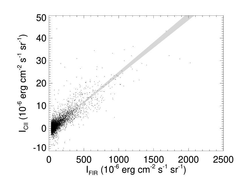
Figure 1: High Galactic latitude [C II] emission is correlated linearly with $FIR$ emission on the large scale. We plot here the integrated intensity of [C II] (${}^{2}{\rm P}_{\rm\scriptscriptstyle 3/2}\rightarrow{{}^{2}\rm P}_{\rm\scriptscriptstyle 1/2}$) emission from COBE FIRAS Line Emission Maps, ${\rm I}_{\rm\scriptscriptstyle CII}$, as a function of the integrated $FIR$ surface brightness, derived from COBE DIRBE ZSMA 60 and 100µm maps resampled to the $7\arcdeg$ FIRAS grid. The 5523 data points with $|b|>5\arcdeg$ can be fit by a straight line with slope $(2.54\pm 0.03)\times 10^{-2}$. We superimpose a gray wedge on the data that represents the $\pm 3\sigma$ range of expected ($FIR$, ${\rm I}_{\rm\scriptscriptstyle CII}$) pairs.

We created DIRBE maps of $FIR$ using the 60 and 100µm ZSMA data, resampled to the 7° FIRAS grid, and compared with the [C II] map (see Figure 1). We obtain a highly significant correlation (there is less than 0.05% chance that the data are uncorrelated). A linear fit weighted by the error bars for all data with $|b|>5\arcdeg$ gives

$${\rm I}_{\rm\scriptscriptstyle CII}=(2.54\pm 0.03)\times 10^{-2}FIR-(1.1375\pm 0.0004)\times\,10^{-6}\,{\rm erg}\,{\rm cm}^{-2}\,{\rm s^{-1}}\,{\rm sr}^{-1},$$ (2)

where ${\rm I}_{\rm\scriptscriptstyle CII}$ and $FIR$ are in the same units. A grey wedge on Figure 1 shows the $3\sigma$ range of expected $FIR$ and ${\rm I}_{\rm\scriptscriptstyle CII}$values. Since the fit was weighted by the COBE error bars, this wedge is much narrower than the actual scatter in data points (the rms scatter in ${\rm I}_{\rm\scriptscriptstyle CII}$ about the fit is $5.29\times\,10^{-6}\,{\rm erg}\,{\rm cm}^{-2}\,{\rm s^{-1}}\,{\rm sr}^{-1}$). The fit gave an ${\rm I}_{\rm\scriptscriptstyle CII}$-intercept of $-1.1375\times\,10^{-6}\,{\rm erg}\,{\rm cm}^{-2}\,{\rm s^{-1}}\,{\rm sr}^{-1}$, because many of the FIRAS [C II] values for low $FIR$ are negative. For what follows, we assume that in the absence of $FIR$ emission there is no [C II] emission, and ignore the intercept.

We compare the [C II]-$FIR$ relationship for “COBE clouds” with our HLC data. The C II integrated intensities of the 101 HLC positions detected with ISO are plotted as a function of the $FIR$ surface brightness in Figure 2. Linear regression to the data, weighted by the errors, gives

$${\rm I}_{\rm\scriptscriptstyle CII}=(2.5\pm 0.9)\times 10^{-2}FIR.$$ (3)

In the fit we have fixed the ${\rm I}_{\rm\scriptscriptstyle CII}$-intercept at zero to reflect our assumption that ${\rm I}_{\rm\scriptscriptstyle CII}=0$ when $FIR=0$. We plot the fit as a solid line in Figure 2. A gray wedge labeled “COBE” represents the $\pm 3\sigma$ range of expected ($FIR$, ${\rm I}_{\rm\scriptscriptstyle CII}$) values based on the COBE data (Equation 2). The HLC and COBE slopes are identical. Our analysis is consistent with the HLCs being part of the same population of sources as the average CNM source observed with the low-resolution COBE instruments.

There is evidence that at the ISO resolution a straight line is not the best representation of the ${\rm I}_{\rm\scriptscriptstyle CII}$-$FIR$ data. Breaking the data into $FIR$ subregions and performing separate linear fits yields a systematic decrease in slope as $FIR$ increases. Figure 3 shows an example of this for bins of width $10^{-4}\,{\rm erg}\,{\rm cm}^{-2}\,{\rm s^{-1}}\,{\rm sr}^{-1}$ along the $FIR$-axis. The local slope is close to the overall slope for $FIR\lesssim 2\,\times 10^{-4}\,\,{\rm erg}\,{\rm cm}^{-2}\,{\rm s^{-1}}\,{\rm sr}^{-1}$, but is virtually zero for $FIR\gtrsim 2\,\times 10^{-4}\,\,{\rm erg}\,{\rm cm}^{-2}\,{\rm s^{-1}}\,{\rm sr}^{-1}$. We also plot in Figure 3 the weighted mean values of ${\rm I}_{\rm\scriptscriptstyle CII}$ and $FIR$ in the bins. A significant departure from the COBE and ISO predictions is seen in the bin with the largest $FIR$ integrated surface brightness, where ${\rm I}_{\rm\scriptscriptstyle CII}$ is 25% lower than expected. Thus, the [C II] emissivity of HLC gas decreases as $FIR$ increases. In §4 we explain this using a model of the radiative heating and cooling of translucent clouds.

3.2 The 60/100 color

Ingalls et al. (2000) showed that the eight HLCs they studied have typical 60/100 colors (${\rm I}_{\rm\scriptscriptstyle 60}$/${\rm I}_{\rm\scriptscriptstyle 100}$) when compared to COBE clouds. The 60/100 colors for our nine clouds are likewise typical. We plot ${\rm I}_{\rm\scriptscriptstyle 100}$ as a function of ${\rm I}_{\rm\scriptscriptstyle 60}$ for our sample in Figure 4. Superimposed on the plot is a dashed line representing the average behavior for Milky Way gas correlated with H I emission, ${\rm I}_{\rm\scriptscriptstyle 60}=0.16\,{\rm I}_{\rm\scriptscriptstyle 100}$ (Dwek et al., 1997). Most positions fall slightly below this line. These sources probably contain mostly atomic gas, since their $FIR$ surface brightnesses are low and their ${\rm I}_{\rm\scriptscriptstyle 60}$/${\rm I}_{\rm\scriptscriptstyle 100}$ ratios are slightly “warmer” than that of average H I. For ${\rm I}_{\rm\scriptscriptstyle 100}>4\,{\rm MJy}\,{\rm sr}^{-1}$ there is a split into two populations: the “cold” sources with ${\rm I}_{\rm\scriptscriptstyle 60}<0.16\,{\rm I}_{\rm\scriptscriptstyle 100}$; and the “warm” sources with ${\rm I}_{\rm\scriptscriptstyle 60}\gtrsim 0.16\,{\rm I}_{\rm\scriptscriptstyle 100}$.

Warm positions generally produce less emission than cold positions—over 90% of the warm positions, but less than 30% of the cold positions, have $FIR<2\times 10^{-4}\,{\rm erg}\,{\rm cm}^{-2}\,{\rm s^{-1}}\,{\rm sr}^{-1}$. Their [C II] and $FIR$ properties are not easily distinguishable otherwise. Weighted linear fits to the [C II] vs. $FIR$ data, holding the intercept fixed at zero, give slopes of $(2.6\pm 1.1)\times 10^{-2}$ for warm sources and $(2.2\pm 1.7)\times 10^{-2}$ for cold sources. These slopes are equivalent within the errors to each other, and to the slope determined for the sample as a whole.

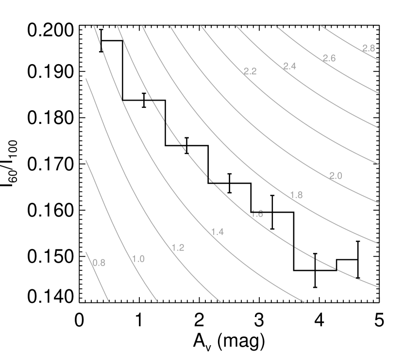
Figure 5: The surface brightness ratio, ${\rm I}_{\rm\scriptscriptstyle 60}$/${\rm I}_{\rm\scriptscriptstyle 100}$  decreases as a function of visual extinction for cloud MBM–12. Image data for over 2,000 pixels are averaged in bins of width $\Delta{\rm A}_{\rm v}=0.71\,$mag. Note that a small adjustment in 60/100 represents a large change in ${\rm A}_{\rm v}$. Models of the thermal emission from dust grains in clouds immersed in the interstellar radiation field (see §4.3.3) are represented as gray curves. The contours are labeled with $\chi_{0}$, the total ISRF flux measured in units of the local value.

The most striking difference between cold and warm positions seems to be their column density. Figure 5 shows this for high–latitude cloud MBM–12 (L1457). Here we compare the 60 and 100µm images to a visual extinction map of the cloud. The extinction, ${\rm A}_{\rm v}$, was derived using an adaptive grid star count algorithm (Cambreśy et al., 1997) from H and K images in the 2MASS second incremental data release. After resampling the 60µm, 100µm, and ${\rm A}_{\rm v}$ images onto the same grid, we compared the 60/100 color with ${\rm A}_{\rm v}$ for each pixel. Figure 5 shows ${\rm I}_{\rm\scriptscriptstyle 60}$/${\rm I}_{\rm\scriptscriptstyle 100}$ averaged in bins of width $\Delta{\rm A}_{\rm v}=0.71\,$mag. The 60/100 color decreases monotonically with increasing extinction, implying that warm dust emission is a characteristic of low extinction positions, while cold dust emission is a characteristic of high extinction positions. The effect is not slight. A small adjustment in 60/100, e.g., from 0.184 to 0.160, represents a large change in ${\rm A}_{\rm v}$, from approximately 1 to 3.

In what follows, we develop a model for the radiative transfer of the ISRF in translucent clouds. This allows us to predict the emission from dust grains, as well as the photoelectric heating and [C II] cooling of the gas. We show that the cold/warm dichotomy in translucent clouds is probably caused by the attenuation of the ISRF, not changes in dust properties.

4 Modeling the C II and FIR emission of HLCs

The [C II] emissivity towards translucent HLCs decreases as the $FIR$ surface brightness increases. The cold and warm populations of HLC positions, identified via their 60/100 colors, have different column densities, and hence different amounts of atomic versus molecular gas, but similar [C II]-$FIR$ emission properties. To explain these empirical facts we offer a model of the heating and cooling of gas and dust in the interstellar medium. The model describes regions heated primarily by the interstellar radiation field, i.e., translucent regions. We simplify the calculations by treating only the single most important sources of heating and cooling of translucent gas: the photoelectric effect for gas heating, and [C II] emission for gas cooling (Wolfire et al., 1995). We predict the $FIR$ and [C II] emission under conditions of thermal equilibrium. For the dust grains, this requires that the power emitted by each grain equals the power absorbed from the attenuated interstellar radiation field. For the gas this requires that the local [C II] cooling rate equals the photoelectric heating rate.

By assuming that [C II] emission is tied to photoelectric heating, we bypass chemistry. We do not attempt to determine the abundance of C II gas in the [C II]-emitting regions, e.g., by balancing the production and destruction of C II using a chemical model. Instead we determine the photoelectric heating, which depends on the dust properties, and equate it with the [C II] cooling modified by an efficiency parameter (e.g., see Bakes & Tielens, 1994). This approximation assumes that (1) most [C II] cooling takes place in FUV-heated areas and (2) most FUV heating takes place in areas cooled by [C II] emission.

If C II were abundant in regions not heated by the photoelectric effect, then much of the [C II] emission might be the result of another heating mechanism, such as cosmic rays, and we would underestimate ${\rm I}_{\rm\scriptscriptstyle CII}$. This is unlikely. If the radiation field is too weak to ionize dust grains (average work function: 5.5$\,{\rm eV}$), it is also too weak to ionize C I (ionization potential: 11.3$\,{\rm eV}$) and form C II. In other words, where there is [C II] cooling, it is the result of FUV heating.

The second tier of our approximation maintains that most photoelectric heating occurs in regions cooled by [C II] emission. If this did not hold, then the emission from another species like C I or CO might provide most of the cooling in some FUV-heated regions and our ${\rm I}_{\rm\scriptscriptstyle CII}$ predictions would be overestimates. It is certainly true that C I and CO are important coolants of translucent clouds, but in terms of total flux the [C I] and CO lines are much weaker than the [C II] line. The brightest known HLC source of [C I], MBM–12, has a maximum observed [C I] (${}^{3}{\rm P}_{\rm\scriptscriptstyle 1}\rightarrow{{}^{3}\rm P}_{\rm\scriptscriptstyle 0}$) integrated intensity of about $3.6\times 10^{-7}\,{\rm erg}\,{\rm cm}^{-2}\,{\rm s^{-1}}\,{\rm sr}^{-1}$ (Ingalls, Bania, & Jackson, 1994), a factor of 10 weaker than the [C II] emission towards most of our HLCs. According to the photodissociation region models of Kaufman et al. (1999), the other [C I] fine structure transition, (${}^{3}P_{2}\rightarrow^{3}P_{1}$), should have at most twice the power of the (${}^{3}{\rm P}_{\rm\scriptscriptstyle 1}\rightarrow{{}^{3}\rm P}_{\rm\scriptscriptstyle 0}$) transition under translucent conditions (FUV flux equal to the local interstellar value and gas volume density $\sim 10^{2-5}\,{\rm cm}^{-3}$). Even if all of the C I atoms that emit in these transitions were excited by FUV-ejected electrons, the photoelectric heating in the [C I]-emitting regions of HLCs is still at most only 30% of that in the [C II]-emitting areas. Furthermore, CO cooling is almost an order of magnitude weaker than [C I] cooling for translucent clouds (eg., see Ingalls et al., 2000). Thus, where there is significant FUV heating, most of the cooling is by [C II] radiation.

4.1 The penetration of the interstellar radiation field into translucent clouds

Here we calculate the intensity spectrum of the interstellar radiation field inside a model cloud, as it is attenuated and processed by dust grains. We adopt a plane parallel geometry, where changes in the mean radiative properties of the gas and dust are dependent only on the optical depth, $\tau_{\lambda}$, measured from the surface of the cloud to the center. The cloud size is defined by the central optical depth, $\tau_{c,\lambda}$.

The interstellar radiation field, $J_{{\rm\scriptscriptstyle ISRF},\lambda}$, is isotropic and incident on both sides of our plane parallel clouds. We consider only the stellar component of the ISRF longward of 0.0912µm (the Lyman continuum), and the cosmic background radiation field. We use the ISRF approximation of Mezger, Mathis, & Panagia (1982) and Mathis, Mezger, & Panagia (1983), which is the sum of a stellar UV component and three diluted blackbodies. We add to this the cosmic background radiation field, $B_{\lambda}(2.7\,{\rm K})$, where $B_{\lambda}(T)$ is the Planck function. We calculate the integrated intensity of the interstellar radiation field to be

$$\int_{0.0912\micron}^{1000\micron}4\pi J_{{\rm\scriptscriptstyle ISRF},\lambda}d\lambda=2.76\times 10^{-2}\,{\rm erg}\,{\rm cm}^{-2}\,{\rm s^{-1}}.$$ (4)

This is 27% higher than the value quoted by Mathis, Mezger, & Panagia (1983), partly because we consider a larger range of wavelength than they did. In constructing an ISRF, we do not include clouds themselves as infrared sources. Infrared photons have little affect on the energetics of translucent clouds because the clouds are transparent to them. Furthermore, the interstellar infrared spectrum results from the processing of stellar radiation by clouds, and does not represent a new source of energy. A goal of this paper is to calculate the infrared spectrum of translucent clouds, to compare with observations.

We use the technique of Flannery, Roberge, & Rybicki (1980) to model the penetration of the ISRF into interstellar clouds. They expressed analytically the solution of the radiative transfer equation in the presence of scattering using a spherical harmonics method. The mean intensity of the radiation field at depth $\tau_{\lambda}$, for a cloud of size $\tau_{c,\lambda}$ is:

$$J_{\lambda}(\tau_{\lambda},\tau_{c,\lambda},\chi_{0}) = \sum_{m=1}^{M}A_{m,\lambda}(\chi_{0})$$ (5)

$$\times\left\{\exp[-k_{m,\lambda}\,\tau_{\lambda}]+\exp[-k_{m,\lambda}\,(2\tau_{c,\lambda}-\tau_{\lambda})]\right\}.$$

The units of $J_{\lambda}$ are erg$\,{\rm s^{-1}}\,{\rm cm}^{-2}\,{\rm sr}^{-1}\,\micron^{-1}$. The coefficients, $A_{m,\lambda}(\chi_{0})$, are determined using the boundary condition at $\tau_{\lambda}=0$, i.e., $J_{\lambda}(0,\tau_{c,\lambda},\chi_{0})\equiv\chi_{0}\,J_{{\rm\scriptscriptstyle ISRF},\lambda}$, whence:

$$A_{m,\lambda}(\chi_{0})=\frac{\chi_{0}\,J_{{\rm\scriptscriptstyle ISRF},\lambda}}{\left[1+\exp(-2k_{m,\lambda}\,\tau_{c,\lambda})\right]M}.$$ (6)

The multiplicative factor, $\chi_{0}$, allows for variations in the nominal radiation field (Mezger, Mathis, & Panagia, 1982; Mathis, Mezger, & Panagia, 1983). The scattering modifiers, {$k_{m,\lambda}$}, are the reciprocal eigenvalues of an $M\times M$ tridiagonal symmetric matrix, X, given by Equation (A3) of Flannery, Roberge, & Rybicki (1980). If we use the scattering phase function introduced by Henyey & Greenstein (1941), then the matrix elements are functions only of the dust grain albedo, $\langle\omega_{\lambda}\rangle$, and the mean cosine of the scattering angle, $\langle g_{\lambda}\rangle$. The $\langle\rangle$ notation we use denotes an average of dust optical properties over the grain population (see Appendix). The $l$th off-diagonal element of the matrix, $X_{l,l+1}$, equals $l/\sqrt{h_{l-1}h_{l}}$, where

$$h_{l}=(2l+1)(1-\langle\omega_{\lambda}\rangle\langle g_{\lambda}\rangle^{l}).$$ (7)

The matrix is symmetric, so $X_{l+1,l}=X_{l,l+1}$. In practice we truncate the series in Equation 5 to $M=20$ terms, since for the wavelengths of interest $k_{21}$ is less than 1% of the value of $k_{20}$. Therefore, X is a $20\times 20$ matrix.

Equation 5 takes as inputs the optical depth, $\tau_{\lambda}$, and the total size of the cloud, given by $\tau_{c,\lambda}$, but we can switch our depth scale to that of the visual extinction, ${\rm A}_{\rm v}=1.086\tau_{\rm\scriptscriptstyle v}$. The visual extinction is a convenient depth scale because it can be related linearly to the column density of hydrogen nuclei, ${\rm N}_{\rm\scriptscriptstyle H}$ (eg., Bohlin, Savage, & Drake, 1978). It can be defined in terms of the wavelength–dependent optical depth using the extinction curve (see Equation A2):

$${\rm A}_{\rm v}=1.086\tau_{\lambda}\,\left(\frac{A_{\lambda}}{{\rm A}_{\rm v}}\right)^{-1}.$$ (8)

The central visual extinction, ${\rm A}_{\rm v,c}$, can be defined similarly in terms of $\tau_{c,\lambda}$.

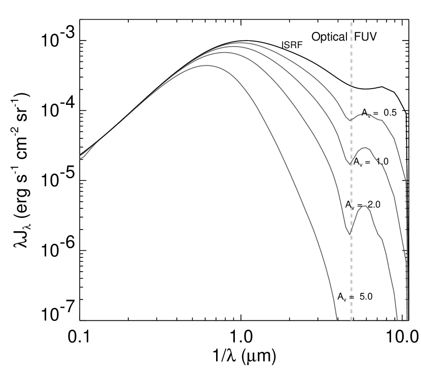
Figure 6: The interstellar radiation field (ISRF) and the attenuated spectrum for four model clouds. The top curve shows the ISRF spectrum as given by Mezger, Mathis, & Panagia (1982) and Mathis, Mezger, & Panagia (1983), plus the 2.7$\,{\rm K}$ cosmic background. This curve defines $\chi_{0}=1$. The lower curves plot the wavelength-weighted mean intensity of the radiation field at the centers of model clouds with central visual extinction, ${\rm A}_{\rm v,c}$, equal to 0.5, 1.0, 2.0, and 5.0 magnitudes. A dashed vertical line at $\lambda=0.2066\micron$, or photon energies of 6$\,{\rm eV}$, denotes the optical/far-ultraviolet (FUV) transition. Photoelectric heating occurs to the right of this line.

We have used Equation 5 to calculate the mean intensity spectrum inside interstellar clouds (Figure 6). In what follows, we use the Equation 5 attenuated radiation field to compute the heating function for dust grains and the photoelectric heating function for the gas. Our assumption of thermal equilibrium then allows us to estimate the surface brightness of 100µm and 60µm radiation from the dust and the [C II] emission line cooling of the gas.

4.2 Dust and gas heating

4.2.1 Thermal equilibrium of dust grains

The temperature of a spherical grain of radius $a$ and material $i$ (see Appendix), measured at depth ${\rm A}_{\rm v}$ in a cloud of central thickness ${\rm A}_{\rm v,c}$, is $T_{g}(a,i,{\rm A}_{\rm v},{\rm A}_{\rm v,c},\chi_{0})$. It can be determined by equating the power absorbed by the grain to the power emitted. This requires:

$$4\pi^{2}a^{2}\int_{0}^{\infty}J_{\lambda}\,Q_{abs,\lambda}(a,i)\,d\lambda=4\pi^{2}a^{2}\int_{0}^{\infty}B_{\lambda}(T_{g})\,Q_{abs,\lambda}(a,i)\,d\lambda,$$ (9)

where $B_{\lambda}(T)$ is the Planck function and $Q_{abs,\lambda}(a,i)$ is the absorption efficiency (see Appendix). The assumption here is that dust grains are in thermal equilibrium. This holds for grains with sizes $a\gtrsim 250\AA$, but breaks down for smaller particles, which are stochastically heated (See Draine & Li 2001, and references therein). We show in §5.3.1 that this equilibrium approach does not affect significantly our conclusions.

We have solved Equation 9 numerically for the function $T_{g}(a,i,{\rm A}_{\rm v},{\rm A}_{\rm v,c},\chi_{0})$. As an example, we plot in Figure 7 the equilibrium temperature of a graphite ($i=1$) grain of size $a=0.1\micron$ as a function of ${\rm A}_{\rm v}$, for a cloud with ${\rm A}_{\rm v,c}=1.0\,$mag, immersed in a $\chi_{0}=1$ interstellar radiation field. At the surface of the cloud, a 0.1µm graphite grain has an equilibrium temperature of $T_{g}\approx 21\,$K. This is comparable to the value independently computed by Li & Draine (2001) for “diffuse clouds,” i.e., clouds without ISRF attenuation. For all grain sizes $\gtrsim 0.01\micron$ and for both graphite and silicate particles, our values of $T_{g}$ at the surfaces of clouds match those of Li & Draine. Our model, which computes the grain temperatures as a function of cloud size, depth, and $\chi_{0}$, can be used to extend the Li & Draine model to the translucent regime, where radiative transfer is important. Figure 6 shows how the spectral shape of the radiation field is already significantly different at the center of an ${\rm A}_{\rm v,c}=1$ cloud from that at the surface. Obviously for translucent clouds, a depth-dependent approach to computing grain temperatures is necessary.

4.2.2 Photoelectric heating of gas

The most important way to transfer energy from the ISRF to the gas is via the photoelectric effect on dust grains. Photoelectric heating of the gas can occur when photons with energies larger than the grain work function expel electrons. A typical neutral grain work function is $\sim 5.5\,{\rm eV}$, so it is mainly FUV photons ($6\,{\rm eV}<h\nu<13.6\,{\rm eV}$ ; $0.2066\micron>\lambda>0.0912\micron$) that contribute to the photoelectric effect. The photoelectric heating mechanism has been explored in detail by Bakes & Tielens (1994). They found that a fraction, $\epsilon$, of the total FUV energy absorbed by all grains is available as photoelectron kinetic energy to heat the gas. The value of $\epsilon$, the “photoelectric heating efficiency,” is expected to be $\sim 3\%$ for neutral grains (Bakes & Tielens, 1994). This can be explained using a simple heuristic argument. An average FUV photon has energy of 8$\,{\rm eV}$, which causes an electron with 2.5$\,{\rm eV}$ of kinetic energy to be released from a neutral grain with work function 5.5$\,{\rm eV}$. In other words, 30% of the incoming photon’s energy is liberated. The typical photoelectric yield is 10%, i.e., 10% of all photons absorbed by grains actually ionize them. Therefore, the fraction of photon energy absorbed that gets injected into the gas as kinetic energy is $\epsilon\sim 0.1\times 0.3=0.03$.

The neutral grain photoelectric efficiency is an upper limit to the actual value of $\epsilon$. For ionized grains, the work functions are higher than 5.5$\,{\rm eV}$, and $\epsilon$ is less than the neutral grain limit. In the cold neutral medium, less than 50% of grains with $a\lesssim 15\AA$ are expected to be ionized (Li & Draine, 2001; Weingartner & Draine, 2001), implying relatively high photoelectric efficiency in translucent clouds.

We used our cloud model to estimate the gas heating in translucent clouds. To compute the total amount of FUV energy absorbed by grains we first estimated the mean absorption cross section per H atom as a function of wavelength, $\langle\sigma_{\lambda}\rangle$:

$$\langle\sigma_{\lambda}\rangle=\sum_{i=1}^{2}\int_{3.2\AA}^{a_{\rm\scriptscriptstyle max}}\pi a^{2}\,C_{i}\,Q_{abs,\lambda}(a,i)\,a^{-3.5}\,da,$$ (10)

where $\{C_{i}\}$ and $a_{\rm\scriptscriptstyle max}$ are defined in the Appendix. Bakes & Tielens (1994) estimated that approximately one half of the heating in interstellar clouds is caused by tiny carbon grains and Polycyclic Aromatic Hydrocarbons (PAHs) with sizes less than 15Å, and the other half comes from larger grains with $15\AA<a<0.01\micron$. The size distribution in the Mathis, Rumpl, & Nordsieck (1977) model (Equation A1) has a minimum cutoff, $a_{\rm\scriptscriptstyle min}=0.005\micron$, so we had to extend the grain parameter calculations of Draine & Lee (1984) to include smaller graphite grains. Following Bakes & Tielens (1994), we assumed that for grains with $a\ll\lambda$ (the Rayleigh limit) the absorption and scattering efficiencies for graphite grains, $Q_{abs,\lambda}(a,1)$ and $Q_{sca,\lambda}(a,1)$, respectively, scale with grain volume. We also assumed that the mean scattering cosine for graphite, $g_{\lambda}(a,1)$, follows the Mie expansion given in Laor & Draine (1993, their Equation 8).

The local gas heating function, $\Gamma$, is derived by integrating the mean intensity of the local radiation field, weighted by the absorption cross section per H atom and the photoelectric efficiency, over all FUV wavelengths and solid angles:

$$\Gamma=4\pi\epsilon\,\int_{0.0912\micron}^{0.2066\micron}J_{\lambda}\,\langle\sigma_{\lambda}\rangle\,d\lambda.$$ (11)

The units of $\Gamma$ are erg$\,\,{\rm s^{-1}}\,({\rm H~{}atom})^{-1}$. In Figure 7 we show the behavior of $\Gamma$ as a function of ${\rm A}_{\rm v}$ for a cloud with ${\rm A}_{\rm v,c}=1.0\,$mag, $\epsilon=0.043$, and $\chi_{0}=1$. Near the surface of the cloud (${\rm A}_{\rm v}\sim 0.3\,$mag), the heating from our model equals the average cooling observed with COBE for high–latitude H I gas, $2.65\times 10^{-26}\,{\rm erg}\,{\rm s^{-1}}\,({\rm H~{}atom})^{-1}$ (Bennett et al., 1994).

4.3 Dust and gas cooling

The grain temperature and the gas heating function allow us to derive the $FIR$ intensity and the [C II] intensity, respectively, towards translucent clouds to compare with observations of these important cooling sources. In the context of our proposed model these are the sole mechanisms of cooling.

4.3.1 FIR Emission

Integrating over the grain distribution, the local cooling function of dust by thermal emission is:

$$\Lambda_{{\rm\scriptscriptstyle d},\lambda}=\sum_{i=1}^{2}\int_{a_{\rm\scriptscriptstyle min}}^{a_{\rm\scriptscriptstyle max}}B_{\nu}(T_{g})\,\pi a^{2}\,Q_{abs,\lambda}(a,i)\,a^{-3.5}\,da,$$ (12)

where

$$\frac{B_{\nu}(T)}{\,{\rm MJy}\,{\rm sr}^{-1}}=\frac{3.97\times 10^{-11}}{{\rm exp}(1.44\times 10^{-4}\micron\cdot\,{\rm K}/\lambda\,T)-1}$$ (13)

is the Planck function. Since $B_{\nu}[T]$ is in $\,{\rm MJy}\,{\rm sr}^{-1}$, the units of $\Lambda_{\rm\scriptscriptstyle d}$ are $\,{\rm MJy}\,{\rm sr}^{-1}\cdot\,{\rm cm}^{2}\,({\rm H~{}atom})^{-1}$. This is equivalent to $\,{\rm MJy}\,{\rm sr}^{-1}$ per H column density, ${\rm N}_{\rm\scriptscriptstyle H}$. The emergent thermal dust emission spectrum can be derived by converting to $\,{\rm MJy}\,{\rm sr}^{-1}$ per ${\rm A}_{\rm v}$  using the standard relation, ${{{\rm N}_{\rm\scriptscriptstyle H}}}\,(\,{\rm cm}^{-2})=1.87\times 10^{21}{\rm A}_{\rm v}\,({\rm mag})$, integrating $\Lambda_{\rm\scriptscriptstyle d}$ from the surface of the cloud to the center, and multiplying by 2:

$$I_{\lambda}({\rm A}_{\rm v,c},\chi_{0})=3.74\times 10^{21}\int_{0}^{{\rm A}_{\rm v,c}}\Lambda_{{\rm\scriptscriptstyle d},\lambda}({\rm A}_{\rm v},{\rm A}_{\rm v,c},\chi_{0})\,d{\rm A}_{\rm v}.$$ (14)

The factor 2 is necessary because the integral is from the edge to the center of a symmetrical one-dimensional cloud.

4.3.2 FIR Spectra

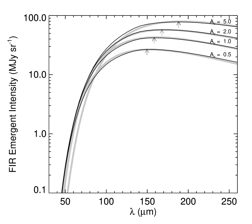
Figure 8: The far-infrared (FIR) surface brightness spectra for thermal equilibrium dust emission from model clouds. Shown here are the spectra for clouds with $\chi_{0}=1$ and ${\rm A}_{\rm v,c}=0.5$, 1.0, 2.0, and 5.0 magnitudes. Vertical arrows indicate the peak of each curve, demonstrating that more optically thick clouds appear “colder.” Thick gray curves show modified blackbody emission for clouds with the same values of ${\rm A}_{\rm v,c}$, but with constant “dust temperature,” $T_{d}=$19, 18, 16.9, and 15.1 K, respectively. Dust emissivity is assumed to vary as $\lambda^{-2}$.

Model FIR spectra, $I_{\lambda}({\rm A}_{\rm v,c},\chi_{0})$, are plotted in Figure 8 for $\chi_{0}=1$. To check our model for internal consistency, we realize that the integrated FIR emission should be less than or equal to the incident ISRF integrated intensity, $2.76\times 10^{-2}\,{\rm erg}\,{\rm cm}^{-2}\,{\rm s^{-1}}$ (Equation 4). For ${\rm A}_{\rm v,c}=(0.5,1.0,2.0,5.0)$, the integrated FIR flux from the clouds is $(1.00,1.53,2.03,2.64)\times 10^{-2}\,{\rm erg}\,{\rm cm}^{-2}\,{\rm s^{-1}}$. Thus, only for extremely opaque clouds ($2{\rm A}_{\rm v,c}\sim 10.0\,$mag) is most of the input radiation recovered as FIR emission, and the input flux is never exceeded.

We can use Figure 8 to predict that clouds with large ${\rm A}_{\rm v,c}$ appear “colder” than clouds with small ${\rm A}_{\rm v,c}$, provided $\chi_{0}$ is held constant. The long wavelength spectrum mimics the emission by dust at a single temperature. Thick gray curves in Figure 8 show modified blackbody spectra for clouds with the same sizes (values of ${\rm A}_{\rm v,c}$) as the model clouds, but with different “dust temperatures,” $T_{d}=$(19,18,16.9,15.1) K, for ${\rm A}_{\rm v,c}=(0.5,1.0,2.0,5.0)$. Here the blackbody function at $T_{d}$ was modified by the dust emissivity, assumed to be proportional to $\lambda^{-2}$. The modified blackbody curves reproduce the model spectra quite well for wavelengths longward of the peak.

We find that a thicker cloud produces more emission than a thinner cloud, but its spectrum peaks at a longer wavelength (vertical arrows), yielding a lower “dust temperature,” as shown by the gray curves. The same behavior was noticed for a large sample of high–latitude clouds by Reach, Wall, & Odegard (1998), who found that the average color temperature for dust mixed with HLC atomic gas is $(17.0\pm 0.3)\,{\rm K}$, whereas for dust mixed with HLC molecular gas the average color temperature is $(14.7\pm 0.2)\,{\rm K}$. This happens because, even though opaque clouds absorb more of the ISRF than transparent clouds, most of the dust in their interiors is exposed to an attenuated version of the ISRF that is deficient in high energy photons.

Our model can be used to estimate the 60 and 100µm surface brightness, ${\rm I}_{\rm\scriptscriptstyle 60}$ and ${\rm I}_{\rm\scriptscriptstyle 100}$, towards translucent clouds, as well as the IRAS–derived $FIR$ integrated surface brightness (Equation 1). Figure 9 plots ${\rm I}_{\rm\scriptscriptstyle 60}$, ${\rm I}_{\rm\scriptscriptstyle 100}$, and $FIR$ versus ${\rm A}_{\rm v,c}$ for $\chi_{0}=1$. Note that even though $FIR$ increases with increasing ${\rm A}_{\rm v,c}$, the rise is not linear, i.e., the $FIR$ emissivity ($FIR$/${\rm N}_{\rm\scriptscriptstyle H}$) of translucent clouds decreases with increasing ${\rm N}_{\rm\scriptscriptstyle H}$, as is observed (see Reach, Wall, & Odegard, 1998).

Another way to demonstrate that thicker clouds have “cooler” dust emission is to compare the surface brightness ratio ${\rm I}_{\rm\scriptscriptstyle 60}$/${\rm I}_{\rm\scriptscriptstyle 100}$ with visual extinction, as we have done empirically for MBM-12. Gray curves on Figure 5 show that, in our model, the 60/100 color decreases with ${\rm A}_{\rm v}$ (= 2${\rm A}_{\rm v,c}$) and increases with $\chi_{0}$. The model agrees remarkably well with the MBM-12 data for $\chi_{0}=1.6\pm 0.2$. Such behavior was already noticed and discussed qualitatively for translucent clouds in the Lynds 134 cloud complex (which contains two objects in our sample, MBM-37 and MBM-33) (Laureijs, Clark, & Prusti, 1991; Laureijs et al., 1995). Cuts across the densest regions of L134 (Laureijs et al., 1995) show that the 60/100 color decreases as B-band extinction, $A_{B}$, increases. We have compared the Laureijs et al. L134 data to our model (using $1.4A_{B}\approx{\rm A}_{\rm v}$), and we find a good match for $\chi_{0}=1.4-1.6$ and ${\rm A}_{\rm v}=0-5$. There is a sudden drop in 60/100 for extremely opaque (${\rm A}_{\rm v}>5$) lines of sight towards the L134 complex (Laureijs, Clark, & Prusti, 1991; Laureijs et al., 1995), which the model does not predict. The authors attribute this to a change in dust properties (see §5.3).

4.3.3 [C II] emission

We estimate the [C II] integrated intensity towards translucent clouds. Recall our key assumptions that the gas cools only through emission in the (${}^{2}{\rm P}_{\rm\scriptscriptstyle 3/2}\rightarrow{{}^{2}\rm P}_{\rm\scriptscriptstyle 1/2}$) transition of C II, and that the gas is in thermal equilibrium. We set the cooling, $\Lambda$ (i.e., the [C II] emission per ${\rm N}_{\rm\scriptscriptstyle H}$), equal to the gas heating, $\Gamma$, given by Equation 11. The integrated intensity of the [C II] emission is:

$${\rm I}_{\rm\scriptscriptstyle CII}({\rm A}_{\rm v,c},\chi_{0},\epsilon)=\frac{3.74\times 10^{21}}{4\pi}\,\,\int_{0}^{{\rm A}_{\rm v,c}}\Gamma({\rm A}_{\rm v},{\rm A}_{\rm v,c},\chi_{0},\epsilon)\,d{\rm A}_{\rm v}.$$ (15)

We plot in Figure 9 the [C II] integrated intensity, ${\rm I}_{\rm\scriptscriptstyle CII}$, as a function of ${\rm A}_{\rm v,c}$ for clouds with $\chi_{0}=1$ and $\epsilon=0.043$. The two upper curves highlight the differences between gas and dust heating by interstellar radiation. The qualitative behavior of both curves is the same. That is, both $FIR$ and ${\rm I}_{\rm\scriptscriptstyle CII}$ rise almost linearly, implying linear increases in column-averaged dust and gas heating with extinction; then both curves show a decrease in slope, implying that clouds with central extinction larger than a transition size produce much less emission at depths greater than this size. The effect of reaching the transition sizes is different for the two tracers. The ${\rm I}_{\rm\scriptscriptstyle CII}$ emission becomes flat at ${\rm A}_{\rm v,c}\sim 0.5\,$mag, whereas $FIR$ only shows a decrease in slope, without flattening even for ${\rm A}_{\rm v,c}=2.0\,$mag. In the interior of a translucent cloud the mean integrated intensity of FUV radiation is much smaller than that of optical radiation (refer to Figure 6). Dust grains are heated by ISRF photons of all wavelengths, but photoelectrons, which lead to [C II] emission, are ejected only by FUV photons. Thus, one expects the [C II] emission to extinguish before the $FIR$ emission does.

4.3.4 Linear and Flat Behavior

The model for $FIR$ and [C II] emission depends on three parameters (see Equations 14 and 15): (1) the cloud column density, given by ${\rm A}_{\rm v,c}$; (2) the incident ISRF flux, $\chi_{0}$, in units of the expected flux at the Sun; and (3) the photoelectric heating efficiency, $\epsilon$. We have computed cloud models for ${\rm A}_{\rm v,c}$ ranging from 0 to 5 mag, and $\chi_{0}$ ranging from 0.2 to 4.0. The [C II] results scale linearly with the photoelectric heating efficiency (Equation 11), so it was trivial to vary $\epsilon$.

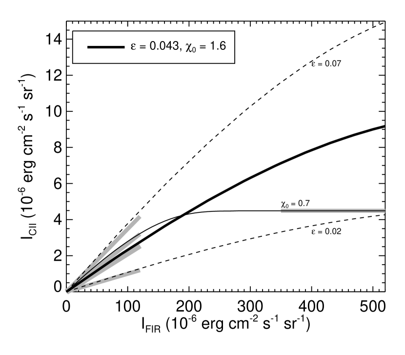
Figure 10: Observables ${\rm I}_{\rm\scriptscriptstyle CII}$ and $FIR$ for model translucent clouds. Each curve shows the behavior as we vary ${\rm A}_{\rm v,c}$, for four combinations of the surface radiation field, $\chi_{0}$, and the photoelectric heating efficiency, $\epsilon$. On the ${\rm I}_{\rm\scriptscriptstyle CII}$–$FIR$ plane, ${\rm A}_{\rm v,c}$ increases from left to right and from bottom to top. The thick solid curve shows the best fit HLC values (see Figure 11), $\chi_{0}=1.6$ and $\epsilon=4.3\%$. The thin solid curve shows the effect of decreasing the ISRF intensity to $\chi_{0}=0.7$, keeping $\epsilon$ fixed at 4.3%. Dashed curves show the effect of changing the heating efficiency from $\epsilon=2\%$ to $7\%$, holding $\chi_{0}$ steady at 1.6. Gray line segments represent the linear portions of the curves and the flat portion of the $\chi_{0}=0.7$ curve, calculated according to the approximations in the text (Equations 16 and 17).

Figure 10 shows plots of ${\rm I}_{\rm\scriptscriptstyle CII}$ as a function of $FIR$ for four different combinations of $\chi_{0}$ and $\epsilon$. The curves show two types of behavior: “linear” behavior for low values of $FIR$; and “flat” behavior for high values of $FIR$. This is due to the difference between dust and gas heating mentioned above. The linear behavior occurs when ${\rm A}_{\rm v,c}$ is low enough that both dust and gas heating increase linearly with ${\rm A}_{\rm v,c}$. The flat behavior occurs when ${\rm A}_{\rm v,c}$ is high enough for FUV heating of the gas to become negligible in cloud interiors, causing [C II] emission to extinguish, but not high enough for optical heating of dust grains to become negligible, so FIR emission is still produced.

We have analyzed models for a range of $\chi_{0}$ and $\epsilon$ values. The behavior of ${\rm I}_{\rm\scriptscriptstyle CII}$ and $FIR$ in the linear regime can be approximated by:

$${\rm I_{\rm\scriptscriptstyle CII}^{\rm\scriptscriptstyle LINEAR}}=FIR\times(0.5634\pm 0.0003)\,\chi_{0}^{-(0.267\pm 0.001)}\,\epsilon.$$ (16)

Errors represent formal uncertainties in fits to the grid of cloud models. The slope of the linear behavior (Equation 16) depends primarily on $\epsilon$ and only weakly on $\chi_{0}$. The slope should not depend at all on $\chi_{0}$, since both ${\rm I}_{\rm\scriptscriptstyle CII}$ and the true FIR integrated intensity should be linearly proportional to $\chi_{0}$. Recall, however, that for comparison with observations we have approximated $FIR$ using ${\rm I}_{\rm\scriptscriptstyle 60}$ and ${\rm I}_{\rm\scriptscriptstyle 100}$ (see Equation 1), i.e., we bias the $FIR$ integral artificially towards short far-infrared wavelengths. As $\chi_{0}$ increases, the short wavelength surface brightness increases faster than linearly, since the peak of the FIR spectrum shifts to shorter wavelengths. Thus our $FIR$ values should also increase with $\chi_{0}$ faster than linearly, while the integrated spectrum increases linearly.

The [C II] intensity in the flat regime can be approximated by:

$$\frac{\rm I_{\rm\scriptscriptstyle CII}^{\rm\scriptscriptstyle FLAT}}{10^{-6}\,\,{\rm erg}\,{\rm cm}^{-2}\,{\rm s^{-1}}\,{\rm sr}^{-1}}=(149.05\pm 0.07)\,\chi_{0}\,\epsilon.$$ (17)

The flatness occurs because at high opacity all incident FUV radiation has been absorbed and converted to photoelectric heating (with efficiency $\epsilon$). The maximum possible [C II] intensity ought to equal the total integrated FUV intensity in the ISRF, multiplied by $\epsilon$:

$$\chi_{0}\,\epsilon\,\int_{0.0912\micron}^{0.2066\micron}J_{{\rm\scriptscriptstyle ISRF},\lambda}d\lambda=1.44\times 10^{-4}\,\chi_{0}\,\epsilon.$$ (18)

Equations 18 and 17 are indistinguishable to within 4%. We superimpose gray line segments on the curves drawn in Figure 10, representing the linear and flat portions of the curves, computed using the approximations in Equations 16 and 17.

We define the transition value of $FIR$ to be the value when ${\rm I_{\rm\scriptscriptstyle CII}^{\rm\scriptscriptstyle LINEAR}}={\rm I_{\rm\scriptscriptstyle CII}^{\rm\scriptscriptstyle FLAT}}$, i.e.,

$$\frac{(FIR)^{\rm\scriptscriptstyle TRANSITION}}{10^{-6}\,\,{\rm erg}\,{\rm cm}^{-2}\,{\rm s^{-1}}\,{\rm sr}^{-1}}=(264.55\pm 0.19)\,\chi_{0}^{(1.267\pm 0.001)}.$$ (19)

The $FIR$ value at which a transition between the linear and flat regimes occurs depends wholly on $\chi_{0}$. We can use Equation 1 to derive a 100µm surface brightness at the linear to flat transition for typical CNM gas (${\rm I}_{\rm\scriptscriptstyle 60}=0.16{\rm I}_{\rm\scriptscriptstyle 100}$):

$$\frac{{\rm I}_{\rm\scriptscriptstyle 100}^{\rm\scriptscriptstyle TRANSITION}}{\,{\rm MJy}\,{\rm sr}^{-1}}=(14.86\pm 0.01)\,\chi_{0}^{(1.267\pm 0.001)}.$$ (20)

4.4 Statistical Comparison of Data with Observations

We can constrain $\epsilon$ and $\chi_{0}$ by comparing our model for the [C II] and $FIR$ emission of translucent clouds to the ISO observations of high–latitude clouds. First we use the simple equations that we derived for the linear, flat, and transition zones. Recall that the observations can be fit by a straight line with slope $2.5\times 10^{-2}$ (Equation 3). This implies that many of the positions observed are in the linear regime. Substitution of the slope into Equation 16 gives $\chi_{0}^{-0.267}\epsilon=0.044$. The binned data, however (Figure 3), show a statistically significant departure from this slope at around $FIR=3\,\times 10^{-4}\,\,{\rm erg}\,{\rm cm}^{-2}\,{\rm s^{-1}}\,{\rm sr}^{-1}$. This appears to be the transition between the linear and flat regimes. Equation 19 gives $\chi_{0}\approx 1.1$, thus $\epsilon\approx 0.045$.

A more sophisticated way to determine $\epsilon$ and $\chi_{0}$ for translucent clouds is to compare a grid of models to the data, and find the best fit. Recall that cloud column density, or central visual extinction, is the independent variable, whereas $FIR$ and ${\rm I}_{\rm\scriptscriptstyle CII}$ are predicted by the model. Given a grid of models, we can “work backwards” from the observed $FIR$ surface brightness to determine ${\rm A}_{\rm v,c}$ as a function of $\epsilon$ and $\chi_{0}$. Effectively $FIR$ becomes the independent variable. The resulting ${\rm A}_{\rm v,c}$ numbers yield a set of predicted [C II] integrated intensities, ${\rm I_{{\rm\scriptscriptstyle CII},i}^{\rm\scriptscriptstyle PREDICTED}}$ that we can compare with the data. We evaluate the “goodness of fit” as a function of $\epsilon$ and $\chi_{0}$:

$$L^{2}\,(\epsilon,\chi_{0})\equiv\sum_{i}\frac{\left(\rm I_{\rm\scriptscriptstyle CII}^{\rm\scriptscriptstyle PREDICTED}-{\rm I_{{\rm\scriptscriptstyle CII},i}}\right)^{2}}{(\sigma_{\rm\scriptscriptstyle CII}^{\rm\scriptscriptstyle PREDICTED})^{2}+\sigma_{{\rm\scriptscriptstyle CII},i}^{2}},$$ (21)

where the sum is over all data points. This is the standard $\chi^{2}$ parameter—we label it $L^{2}$ here so as not to confuse the reader with the ISRF intensity, $\chi_{0}$. Here $\sigma_{\rm\scriptscriptstyle CII}^{\rm\scriptscriptstyle PREDICTED}$ is computed the same way as ${\rm I_{{\rm\scriptscriptstyle CII},i}^{\rm\scriptscriptstyle PREDICTED}}$, using the $FIR$ observed uncertainty range, $FIR_{i}\pm\sigma_{FIR,i}$.

Figure 11 shows contours of constant $L^{2}$ in the ($\epsilon$,$\chi_{0}$) plane, representing 68.3%, 95.4%, and 99.7% confidence in the fit of our model to the data. These are equivalent to the 1, 2, and 3$\sigma$ confidence intervals for Gaussian statistics. The minimum $L^{2}$ point, indicated by a cross in Figure 11, gives the most probable values, $\epsilon=0.043{{+0.010}\atop{-0.002}}$ and $\chi_{0}=1.6$. We derive a lower ($-3\sigma$) limit of $\chi_{0}\geq 1$, but cannot derive an upper limit because the Figure 11 contours of constant $L^{2}$ continue indefinitely in the $\chi_{0}$ dimension. Apparently a complete transition to flat behavior, which determines the value of $\chi_{0}$, does not occur in our HLC dataset.

In terms of $\epsilon$ and $\chi_{0}$, there is only marginal difference between the “warm” and “cold” HLC positions defined in §3. Separate $L^{2}$ analyses for the warm and cold data points yield $\epsilon_{\rm\scriptscriptstyle WARM}=0.053{{+0.003}\atop{-0.007}}$ and $\chi_{0,{\rm\scriptscriptstyle WARM}}\gtrsim 1.0$ ($3\sigma$ lower limit); and $\epsilon_{\rm\scriptscriptstyle COLD}=0.045\pm 0.004$ and $\chi_{0,{\rm\scriptscriptstyle COLD}}\gtrsim 0.8$ ($3\sigma$ lower limit). Within the 1$\sigma$ uncertainties, the $\epsilon$ values are identical. The lower limits on $\chi_{0}$ are consistent with each other. In addition, both the warm and cold 3$\sigma$ confidence contours overlap each other nearly exactly. We conclude that translucent cloud positions with warm and cold IRAS 60/100 colors have nearly the same values of $\epsilon$ and $\chi_{0}$.

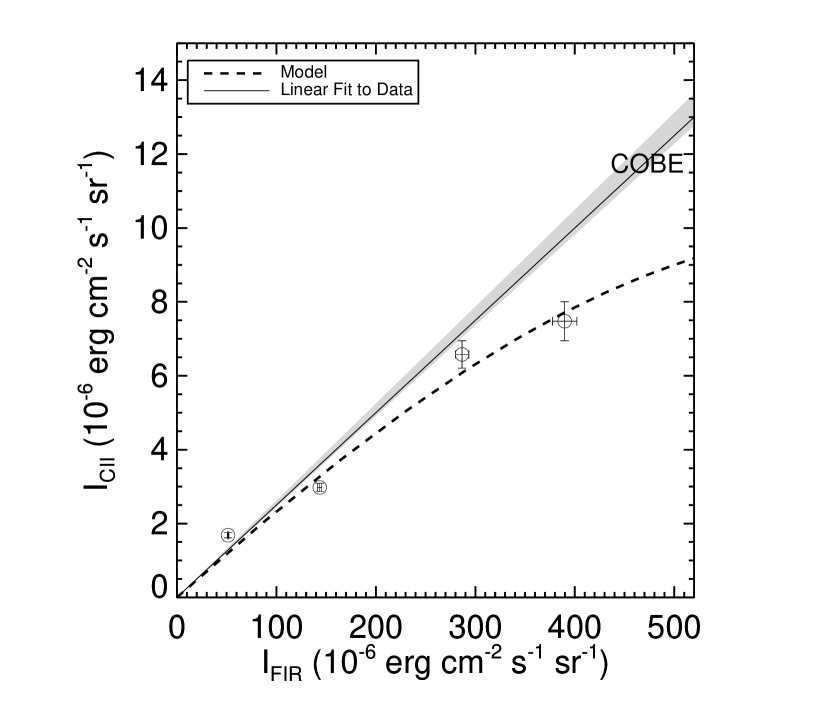
Figure 12: Binned HLC measurements of ${\rm I}_{\rm\scriptscriptstyle CII}$ versus $FIR$ (Figure 3), compared with model results. The gray wedge represents the range of COBE data, as described in the caption to Figure 2. The dashed curve represents the best fit model, $\epsilon=0.043$ and $\chi_{0}=1.6$. A solid line shows the fit to our HLC data (Figure 2).

Figure 12 displays the best fit model for ${\rm I}_{\rm\scriptscriptstyle CII}$ versus $FIR$, superimposed on the binned data from Figure 3. The observed decrease in [C II] emissivity at high values of $FIR$ (Figure 3) is reproduced by the model, signifying that HLCs with $FIR\gtrsim 3\,\times 10^{-4}\,\,{\rm erg}\,{\rm cm}^{-2}\,{\rm s^{-1}}\,{\rm sr}^{-1}$ absorb most incident FUV photons.

5 Discussion

In this paper we have studied the [C II] and far–infrared (FIR) emission towards high–latitude translucent molecular clouds (HLCs). These observational signatures of the processing of the interstellar radiation field (ISRF) by the clouds help to elucidate the role of dust grains in heating the gas.

5.1 The [C II] emissivity and extinction

The chief conclusion to be drawn from the new ISO data is that, for $FIR\lesssim 3\,\times 10^{-4}\,\,{\rm erg}\,{\rm cm}^{-2}\,{\rm s^{-1}}\,{\rm sr}^{-1}$, ${\rm I}_{\rm\scriptscriptstyle CII}$ and $FIR$ are linearly correlated on $\sim 1\arcmin$ scales (Figure 2), confirming the 7$\arcdeg$ COBE FIRAS result, ${\rm I}_{\rm\scriptscriptstyle CII}\propto FIR^{0.95}$, for the Galactic plane (Bennett et al., 1994). The confirmation is not just qualitative: the proportionality constant is the same for both COBE and ISO. At low extinction the $FIR$ integrated intensity is proportional to the H I column density, so the [C II] emissivity is constant for all low-extinction interstellar regions.

The [C II] emissivity decreases for high extinction lines of sight due to the attenuation of FUV photons that cause photoelectric heating, an effect that was unnoticed in the low resolution COBE data. When we bin the data (Figure 3) they show a statistically significant decrease in slope for $FIR\gtrsim 3\,\times 10^{-4}\,\,{\rm erg}\,{\rm cm}^{-2}\,{\rm s^{-1}}\,{\rm sr}^{-1}$. We do not have enough high extinction sources in our sample to be sure that ${\rm I}_{\rm\scriptscriptstyle CII}$ flattens completely, as predicted by our model. At the minimum, there is a link between the decreasing emissivity of [C II] and the transition from mostly “warm” to mostly “cold” values of ${\rm I}_{\rm\scriptscriptstyle 60}$/${\rm I}_{\rm\scriptscriptstyle 100}$, because most warm positions have low $FIR$ intensity and most cold positions have high $FIR$ intensity.

The COBE data do not show a decrease in [C II] emissivity for high values of $FIR$, probably because translucent HLCs are diluted inside the 7° COBE beam. The mean CO emission size of HLCs is $\sim$ 1° (Magnani, Hartmann, & Speck, 1996), but detectable CO emission from HLCs covers less than 3% of the sky (Magnani, et al., 2000). Thus on 7° scales, $\sim 97\%$ of [C II] emission is from purely atomic material, so the COBE survey yields only linear behavior for ${\rm I}_{\rm\scriptscriptstyle CII}$ versus $FIR$. The 70″ ISO beam, on the other hand, is capable of resolving translucent HLCs where the column-averaged [C II] emissivity is much lower than in diffuse H I.

The 60µm/100µm color is often used to infer either the ISRF flux (e.g., Dale et al., 2001) or the grain size distribution (e.g., Laureijs, Clark, & Prusti, 1991), but our work indicates that for translucent clouds variations in ${\rm I}_{\rm\scriptscriptstyle 60}$/${\rm I}_{\rm\scriptscriptstyle 100}$ can be accounted for entirely by variations in the extinction. Thicker clouds appear colder, even if the grain size distribution and the radiation field stay constant. Fitting our model to the ${\rm I}_{\rm\scriptscriptstyle CII}$ and $FIR$ data yields the same values of the photoelectric heating efficiency, $\epsilon$, and the ISRF flux, $\chi_{0}$, for sources with both warm and cold 60/100 colors.

5.2 The ISRF Flux and the Photoelectric Heating Efficiency

The actual best fit values of the ISRF flux and the photoelectric heating efficiency are noteworthy. We found that the most probable bolometric ISRF flux incident on HLCs is $\chi_{0}=1.6$, where $\chi_{0}\equiv 1$ defines the ISRF spectrum of Mezger, Mathis, & Panagia (1982) and Mathis, Mezger, & Panagia (1983). We also derive $\chi_{0}\approx 1.6$ independently for cloud MBM-12 using the observed ${\rm I}_{\rm\scriptscriptstyle 60}$/${\rm I}_{\rm\scriptscriptstyle 100}$ behavior as a function of visual extinction (Figure 5). The FUV portion of a $\chi_{0}=1.6$ field has an integrated flux of $2.9\times 10^{-2}\,{\rm erg}\,{\rm cm}^{-2}\,{\rm s^{-1}}$. In units of the Habing (1968) flux ($1.6\times 10^{-2}\,{\rm erg}\,{\rm cm}^{-2}\,{\rm s^{-1}}$), this gives $G_{0}=1.8$, close to the actual value ($G_{0}=1.7$) determined from space-based UV measurements (Draine, 1978). Given that our model is so successful at determining $G_{0}$, even without observing clouds in the flat regime where all FUV is absorbed, it is likely that the curve in Figure 12 is a realistic representation of the average [C II] and $FIR$ properties of translucent high–latitude clouds. This means that the decrease in [C II] emissivity that we detect is indeed the transition between regions with less than complete and complete FUV absorption, confirming the use of the term “translucent” to describe the HLCs. We predict that the [C II] emissivity should decrease further for HLC positions with higher extinction than those in our current sample.

The photoelectric heating efficiency that we derive, $\epsilon=4.3\%$, is slightly higher than the value 3% derived from COBE data by Bakes & Tielens (1994). Recall that $\epsilon$ is the fraction of far-ultraviolet radiation absorbed by grains that is converted to gas heating. Bakes & Tielens estimated $\epsilon$ for the Galaxy by dividing the observed [C II] integrated intensity by FIR. In so doing, they equated ${\rm I}_{\rm\scriptscriptstyle CII}$ with photoelectric heating, as we do; but they also equated FIR with the absorbed FUV flux, which is only partially true for translucent material. In the cold neutral medium half of the ISRF flux that heats dust grains and causes FIR emission is at optical wavelengths. The FIR integrated surface brightness can only be used to estimate the absorbed FUV flux if clouds have nearby O and B stars, causing FUV photons to dominate the radiation field.

Another way to obtain a crude estimate of $\epsilon$ for the cold neutral medium (CNM) is to consider the limiting case of complete FUV absorption in translucent gas. The [C II] cooling that should result is $I_{\rm\scriptscriptstyle CII}^{\rm\scriptscriptstyle max}=1.44\times 10^{-4}\,\chi_{0}\,\epsilon\,\,{\rm erg}\,{\rm cm}^{-2}\,{\rm s^{-1}}\,{\rm sr^{-1}}$ (Equation 18). For our Figure 2 HLC sample, $I_{\rm\scriptscriptstyle CII}^{\rm\scriptscriptstyle max}\approx 1.1\,\times 10^{-5}\,\,{\rm erg}\,{\rm cm}^{-2}\,{\rm s^{-1}}\,{\rm sr}^{-1}$, so the product $\chi_{0}\,\epsilon\approx 0.076$. Taking $\chi_{0}=1.6$ (see above) gives $\epsilon=4.8\%$, implying that the CNM is extremely efficient at processing FUV radiation. In fact, both the 4.8% estimate and our best fit appraisal, $\epsilon=(4.3{{+1.0}\atop{-0.2}})\%$, are consistent with the value 4.9% adduced as the maximum efficiency for neutral grains (Wolfire et al., 1995; Bakes & Tielens, 1994). Fewer than 50% of the grains responsible for heating the CNM are expected to be ionized (Li & Draine, 2001; Weingartner & Draine, 2001), so the grains should have close to maximal efficiency.

5.3 Limitations in the Grain Model

5.3.1 Thermal Equilibrium Assumption for Very Small Grains

Our results depend on the assumption that all dust grains are in thermal equilibrium. In particular, Equations 9 and 12 require this condition. As mentioned in §4.2.1, thermal equilibrium breaks down for grains smaller than $a\sim 250\AA$, which are heated by individual photons. These very small grains (VSGs) get much hotter than the temperatures we derived by equating the average power absorbed with that emitted. The effect is most obvious at short wavelengths ($\lambda\lesssim 60\micron$). Thus our predicted thermal equilibrium 60µm surface brightnesses are underestimates to the actual values derived when the stochastic heating of very small grains is considered. According to the models of Li & Draine (2001, Figure 8), stochastically heated VSGs are responsible for approximately half of the 60µm flux from diffuse high–latitude clouds (see also Verter et al., 2000). Clearly this is an overestimate to the stochastic VSG contribution to the emission from translucent clouds, since the power absorbed (and hence emitted) by VSGs is a strong function of the FUV flux, which decreases inside translucent clouds. If our predictions for ${\rm I}_{\rm\scriptscriptstyle 60}$ are underestimated by a factor $\lesssim 2$, then our $FIR$ predictions will be underestimated by $\lesssim 20\%$ (using Equation 1 and the fact that ${\rm I}_{\rm\scriptscriptstyle 60}\approx 0.16{\rm I}_{\rm\scriptscriptstyle 100}$ for average H I clouds). Adding 20% to our model $FIR$ values decreases by 20% the slope of the linear ${\rm I}_{\rm\scriptscriptstyle CII}$ vs. $FIR$ relationship for a given ($\epsilon$,$\chi_{0}$) pair. Thus the derived product $\epsilon\chi_{0}^{-0.267}$ (Equation 16) decreases by 20%. This does not change significantly our conclusions, since $\epsilon=0.043{{+0.01}\atop{-0.002}}$ is already uncertain by 23%. We need to take into account the small grain physics in more detail to assess accurately the errors due to our equilibrium approach. This will not change an important conclusion derived from our model: variations in the [C II] emissivity and the 60/100 color in translucent clouds reflect variations in grain heating, not changes in grain optical properties.

5.3.2 Variations in Grain Optical Properties

It is likely that our conclusions will change for extremely opaque clouds, whose interiors may be sufficiently dense and free of UV photons for smaller dust particles to coagulate into larger grains. Two compelling pieces of evidence for variations in the optical properties of grains are (1) an abrupt drop in 60/100 at ${\rm A}_{\rm v}\sim 5$ (e.g., Laureijs, Clark, & Prusti, 1991; Laureijs et al., 1995); and (2) far-infrared spectra indicating an extremely cold ($12-13\,{\rm K}$) population of dust towards dense cores (e.g., Bernard et al., 1999; Juvela et al., 2002). Neither feature is a characteristic of our model, so we caution against applying our conclusions directly to dark clouds. Nonetheless, the effects should be negligible in the model’s intended domain, i.e., translucent clouds (${\rm A}_{\rm v}=1-5$).

5.4 Details of Cloud Structure

In our analysis we made no explicit mention of the cloud density structure. We parametrized our model in terms of the visual extinction, which allows us to ignore density structure along the line of sight. If the volume density varies along the line of sight, the size scale associated with extinction varies, but this does not affect our calculations if all else remains the same, i.e., the photoelectric effect is the major heating source and [C II] emission is the dominant cooling source. This is probably true. The brightest lines observed in HLCs (${\rm I}_{\rm\scriptscriptstyle CII}\sim 1\,\times 10^{-5}\,\,{\rm erg}\,{\rm cm}^{-2}\,{\rm s^{-1}}\,{\rm sr}^{-1}$) account for approximately 5% of the incident FUV flux (when $G_{0}=1.7$; see §5.2 and Draine 1978). In other words, the FUV heating is converted to [C II] cooling with very high efficiency. This probably requires that the [C II] excitation conditions are always thermal, i.e., either the density is above the critical density, ${\rm n}_{\rm\scriptscriptstyle crit}=A_{ul}/\gamma_{ul}$, where $\gamma_{ul}$ is the collisional excitation coefficient; or the temperature is above $h\nu_{ul}/k=91\,{\rm K}$. The average CNM temperature is $\sim 80\,{\rm K}$, but it ranges from 20–200$\,{\rm K}$ (Kulkarni & Heiles, 1987), so the H I gas is probably hot enough for [C II] to be thermalized. For cooler gas ($T\sim 20\,{\rm K}$), the [C II] critical density is high. For excitation by ${\rm H}_{2}$, ${\rm n}_{\rm\scriptscriptstyle crit}\approx 9000\,{\rm cm}^{-3}$; for excitation by H I, ${\rm n}_{\rm\scriptscriptstyle crit}\approx 6700\,{\rm cm}^{-3}$. The CO-emitting molecular regions of HLCs could have such high densities (Ingalls et al., 2000), but it is not clear that the [C II]-emitting regions are so dense. It is probably the case that gas which is too rarefied to be supercritical either is hot enough for [C II] to be thermalized or does not contribute much to the overall extinction. We conclude that the detailed structure along the line of sight therefore has little effect on our analysis.

Structural variations in the plane of the sky are more difficult to account for, for two reasons. First, clouds with structure in three dimensions are more permeable to the interstellar radiation field, especially when one takes into account scattering of FUV photons by dust grains (Spaans, 1996). Second, the emission observed towards clouds is always the result of averaging the real emission across a telescope beam. Comparing two tracers observed with the same beamsize towards the same position minimizes the effects of structured emission. Unfortunately, the IRAS data we use have a resolution of 4′, whereas the ISO [C II] measurements have only 71″ resolution—a factor of 11 in beam area! We probably have enough data points that structural variations averaged out in statistics (compare Figure 2 to Figure 3). Nevertheless, to improve the robustness of our conclusions requires higher resolution FIR observations, perhaps made with the Space Infrared Telescope Facility.

6 Conclusions

A linear relationship is observed between the $FIR$ and [C II] emission for high Galactic latitude molecular clouds observed with ISO that is indistinguishable from the prediction based on high–latitude COBE data, implying that the [C II] emissivity is constant for all low-extinction gas. At high extinction the [C II] emissivity begins to decrease due to the attenuation of the FUV portion of the interstellar radiation field. In contrast to other work, we find that differences in the 60µm/100µm color can be accounted for solely by extinction variations. Sources with both warm and cold colors seem to be exposed to the same radiation field, equal to the mean field near the Sun; and have the same photoelectric heating efficiency, close to the value for neutral grains. The transition from sources with warm to those with cold 60/100 colors coincides approximately with the transition from constant to decreasing [C II] emissivity. Such regions where the FUV spectrum is attenuated and softened, but is still important for heating the gas, define the translucent regime.

Appendix A Deriving Bulk Properties of the Grain Distribution

We assume that grains are spherical with radius $a$, and come in two kinds, graphite ($i=1$) and “astronomical silicate” ($i=2$). The fundamental optical properties of interstellar grains —absorption efficiency, $Q_{abs,\lambda}(a,i)$; scattering efficiency, $Q_{sca,\lambda}(a,i)$; and mean cosine of scattering angle, $g_{\lambda}(a,i)$—have been computed by Draine & Lee (1984) and Laor & Draine (1993). The albedo can be constructed from these basic properties, $\omega=(Q_{sca}/Q_{abs})/[1+(Q_{sca}/Q_{abs})]$.

Following Mathis, Rumpl, & Nordsieck (1977), we assume a power law distribution of grain sizes:

$$dn_{i}=C_{i}a^{-3.5}da,~{}~{}~{}~{}a_{\rm\scriptscriptstyle min}<a<a_{\rm\scriptscriptstyle max},$$ (A1)

where $dn_{i}$ is the number of grains per H atom of type $i$ with radii between $a$ and $a+da$, and the upper and lower size limits are $a_{\rm\scriptscriptstyle max}\approx 0.25\micron$ and $a_{\rm\scriptscriptstyle min}\approx 0.005\micron$, respectively. The coefficients $C$ were determined by Draine & Lee (1984) to be $C_{1}=10^{-25.16}\,{\rm cm}^{2.5}\,({\rm H~{}atom})^{-1}$ for graphite and $C_{2}=10^{-25.11}\,{\rm cm}^{2.5}\,({\rm H~{}atom})^{-1}$ for silicate. The values of the $C_{i}$ coefficients were derived by fitting the theoretical extinction curve (see Equation A2 below) to the observed average extinction curve for the Galaxy (Savage & Mathis, 1979).

Bulk observables can be computed by integrating a particular property over the distribution of grain sizes, $a$ and materials, $i$. For example, to obtain the wavelength-dependent extinction, $A_{\lambda}$, one integrates the extinction cross section, $\sigma_{ext,\lambda}(a,i)=\pi a^{2}Q_{ext,\lambda}(a,i)$ [where $Q_{ext,\lambda}(a,i)\equiv Q_{abs,\lambda}(a,i)+Q_{sca,\lambda}(a,i)$], over the grain distribution:

$$\frac{A_{\lambda}}{{{{\rm N}_{\rm\scriptscriptstyle H}}}}=\sum_{i=1}^{2}C_{i}\,\int_{a_{\rm\scriptscriptstyle min}}^{a_{\rm\scriptscriptstyle max}}\pi a^{2}\,Q_{ext,\lambda}(a,i)\,a^{-3.5}\,da.$$ (A2)

The extinction curve is usually expressed as $A_{\lambda}/{\rm A}_{\rm v}$, which requires that we multiply Equation A2 by the standard relationship between column density and visual extinction ${{{\rm N}_{\rm\scriptscriptstyle H}}}(\,{\rm cm}^{-2})=1.87\times 10^{21}{\rm A}_{\rm v}({\rm mag})$ (Bohlin, Savage, & Drake, 1978).

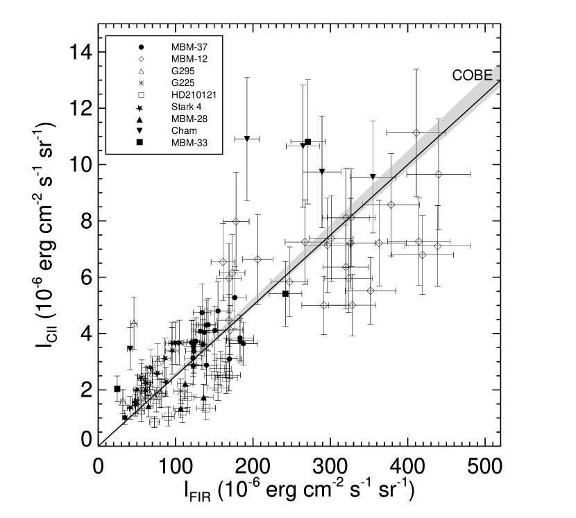
Figure 2: The HLCs are average sources of [C II] and FIR emission. Data points show the ISO integrated intensity of [C II] versus $FIR$ from IRAS observations for 101 positions in 9 high–latitude clouds. The gray wedge labeled “COBE” represents the $\pm 3\sigma$ range of expected ($FIR$, ${\rm I}_{\rm\scriptscriptstyle CII}$) pairs based on fits to the all sky COBE data for $|b|>5\arcdeg$ (see Figure 1). The solid line is a weighted least squares fit to our HLC data, ${\rm I}_{\rm\scriptscriptstyle CII}=2.5\times 10^{-2}FIR$.

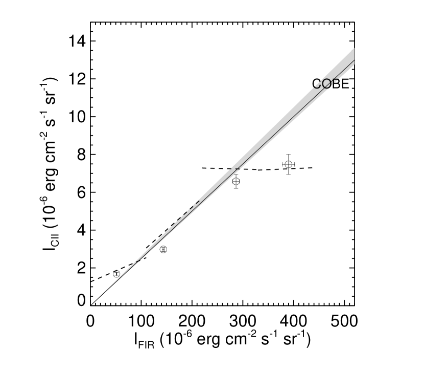
Figure 3: The [C II] emissivity of HLCs decreases as $FIR$ increases. Dashed line segments display weighted linear fits to the HLC data (Figure 2), separated into bins of width $10^{-4}\,{\rm erg}\,{\rm cm}^{-2}\,{\rm s^{-1}}\,{\rm sr}^{-1}$ along the $FIR$-axis. Circles with error bars denote the weighted mean values of ${\rm I}_{\rm\scriptscriptstyle CII}$ and $FIR$ in these bins. The gray wedge represents the range of COBE data for average Milky Way sources, as described in the caption to Figure 2. The solid line is the fit to our HLC data (Figure 2).

Figure 4: Surface brightness at 100µm versus that at 60µm for our HLC sample. A dashed line indicates the mean behavior derived using COBE DIRBE observations of Galactic gas associated with H I, ${\rm I}_{\rm\scriptscriptstyle 60}=0.16\,{\rm I}_{\rm\scriptscriptstyle 100}$ (Dwek et al., 1997). This line is not a fit to the data. We identify two populations based on the 60/100 color: a “warm” population for which ${\rm I}_{\rm\scriptscriptstyle 60}\gtrsim 0.16{\rm I}_{\rm\scriptscriptstyle 100}$; and a “cold” population for which ${\rm I}_{\rm\scriptscriptstyle 60}<0.16{\rm I}_{\rm\scriptscriptstyle 100}$.

Figure 7: The heating of an interstellar cloud with ${\rm A}_{\rm v,c}=1.0\,$mag. The dashed line (right scale) shows the equilibrium temperature of graphite grains of size $a=0.1\micron$, plotted as a function of ${\rm A}_{\rm v}$. The solid line (left scale) shows the gas heating function in the same cloud, assuming the photoelectric efficiency is 4.3%. We only show the profiles for half of the cloud, since the profiles are symmetric about ${\rm A}_{\rm v}={\rm A}_{\rm v,c}$.

Figure 9: The dust and gas cooling towards translucent clouds with $\chi_{0}=1$ and $\epsilon=4.3\%$. The two lower curves (right scale) represent emission in the 60µm and 100µm IRAS bands from thermal dust grains, “observed” toward a set of model clouds with different column density, given by ${\rm A}_{\rm v,c}$. The ${\rm I}_{\rm\scriptscriptstyle 60}$ values have been multiplied by 5 for clarity. The two upper curves (left scale) represent the “FIR” integrated intensity, derived using ${\rm I}_{\rm\scriptscriptstyle 60}$ and ${\rm I}_{\rm\scriptscriptstyle 100}$ (Equation 1); and the [C II] integrated intensity, multiplied by 50 for clarity.

Figure 11: Statistical comparison of observed [C II] integrated intensity and $FIR$ surface brightness with our model, for a grid of $\epsilon$ and $\chi_{0}$ values. Contours (smallest to largest area) show the 1, 2, and 3$\sigma$ confidence intervals in the fit of the model to the data shown in Figure 2. The cross represents the best match, $\epsilon=0.043$ and $\chi_{0}=1.6$.

Table 1: ISO LWS Observations of High-Latitude Clouds

Source Name	$\ell$	$b$	FOV	PA	Detected/
	$(\arcdeg)$	$(\arcdeg)$	$(\arcmin\times\arcmin)$	($\arcdeg$)	Observed
MBM–37	6.007	36.750	$21.0\times 1.2$	90	7/7
(L183)	5.778	36.987	$21.0\times 1.2$	90	7/7
	6.235	36.512	$21.0\times 1.2$	90	7/7
	7.172	37.040	$\phantom{2}1.2\times 1.2$	0	1/1
HD210121	56.876	–44.461	$\phantom{2}1.2\times 1.2$	0	1/1
	56.107	–44.188	$\phantom{2}1.2\times 1.2$	0	1/1
	56.436	–44.147	$\phantom{2}1.2\times 1.2$	0	1/1
	56.511	–44.019	$21.9\times 1.2$	55	8/9
MBM–28	141.755	39.047	$\phantom{2}1.2\times 1.2$	0	1/1
(Ursa Major)	140.784	38.501	$\phantom{2}1.2\times 1.2$	0	0/1
	141.306	39.430	$\phantom{2}1.2\times 1.2$	0	1/1
	142.002	38.700	$\phantom{2}1.2\times 1.2$	0	1/1
	142.070	38.199	$\phantom{2}1.2\times 1.2$	0	1/1
MBM–12	159.251	–34.483	$\phantom{2}1.2\times 1.2$	0	1/1
(L1457)	159.151	–33 817	$\phantom{2}1.2\times 1.2$	0	1/1
	159.301	–33.501	$\phantom{2}1.2\times 1.2$	0	1/1
	159.301	–34.471	$30.0\times 6.0$	135	20/20
	159.401	–34.450	$\phantom{2}1.2\times 1.2$	0	1/1
	159.601	–34.501	$\phantom{2}1.2\times 1.2$	0	2/2
G225.3–66.3	225.274	–66.280	$\phantom{2}1.2\times 1.2$	0	1/1
	225.312	–65.413	$\phantom{2}1.2\times 1.2$	0	0/1
G295.3–36.2	295.311	–36.141	$21.0\times 1.2$	0	6/7
	295.284	–36.123	$21.0\times 1.2$	0	7/7
G300.1–16.6	300.055	–16.620	$\phantom{2}1.2\times 1.2$	0	1/1
(Chamaeleon)	299.674	–16.318	$\phantom{2}1.2\times 1.2$	0	1/1
	299.914	–16.799	$\phantom{2}1.2\times 1.2$	0	1/1
	300.250	–16.955	$\phantom{2}1.2\times 1.2$	0	1/1
	300.263	–16.767	$\phantom{2}1.2\times 1.2$	0	1/1
Stark 4	310.142	–44.475	$18.0\times 1.2$	90	6/9
	309.578	–45.141	$\phantom{2}1.2\times 1.2$	0	0/1
	309.747	–44.579	$18.0\times 1.2$	90	9/9
	309.967	–44.522	$\phantom{2}1.2\times 1.2$	0	1/1
MBM–33	359.150	36.578	$\phantom{2}1.2\times 1.2$	0	1/1
(L1780)	358.897	36.976	$\phantom{2}1.2\times 1.2$	0	1/1
	358.954	36.832	$\phantom{2}1.2\times 1.2$	0	1/1

References

- Bakes & Tielens (1994) Bakes, E. L. O. & Tielens, A. G. G. M. 1994, ApJ, 427, 822
- Bennett et al. (1994) Bennett, C. L. et al., 1994, ApJ, 436, 423
- Bernard et al. (1999) Bernard, J. P. et al., 1999, A&A, 347, 640
- Bohlin, Savage, & Drake (1978) Bohlin, R. C., Savage, B. D., & Drake, J. F. 1978, ApJ, 224, 132
- Boulanger et al. (1996) Boulanger, F., et al., 1996, A&A, 312, 256
- Burgdorf et al. (1998) Burgdorf, M. J. et al., 1998, Advances in Space Research, 21(1), 5
- Caldwell et al. (1998) Caldwell, M. et al., 1998, Proc. SPIE Vol 3426, Scattering and Surface Roughness II, eds Z.-H. Gu and A. A. Maradudin, 313
- Cambreśy et al. (1997) Cambreśy, L., et al., 1997, A&A, 324, L5
- Clegg et al. (1996) Clegg, P. E. et al., 1996, A&A, 315, L38
- Dale et al. (2001) Dale, D. A., Helou, G., Contursi, A., Silberman, N. A., & Kolhatkar, S. 2001, ApJ, 549, 215
- de Jong (1977) de Jong, T. 1977, A&A, 55, 137
- DIRBE (1998) DIRBE Explanatory Supplement 1998, eds M. G. Hauser, T. Kelsall, D. Leisawitz, & J. Weiland, Version 2.3; see also http://space.gsfc.nasa.gov/astro/cobe/
- Draine (1978) Draine, B. T. 1978, ApJS, 36, 59
- Draine & Lee (1984) Draine, B. T. & Lee, H. M. 1984, ApJ, 285, 89
- Draine & Li (2001) Draine, B. T., & Li, A. 2001, ApJ, 551, 807
- Dwek et al. (1997) Dwek, E. et al., 1997, ApJ, 475, 565
- Flannery, Roberge, & Rybicki (1980) Flannery, B. P., Roberge, W., & Rybicki, G. B. 1980, ApJ, 236, 598
- Gir, Blitz, & Magnani (1994) Gir, B.-Y., Blitz, L., & Magnani, L. 1994, ApJ, 434, 162
- Habing (1968) Habing, H. J. 1968, Bull. Astron. Inst. Netherlands, 19, 421
- Helou, Soifer, & Rowan-Robinson (1985) Helou, G., Soifer, B. T., & Rowan-Robinson, M. 1985, ApJ, 298, L7
- Helou et al. (1988) Helou, G., Khan, I. R., Malek, L., & Boehmer, L. 1988, ApJS, 68, 151
- Henyey & Greenstein (1941) Henyey, L. G., & Greenstein, J. L. 1941, ApJ, 93, 70
- Ingalls, Bania, & Jackson (1994) Ingalls, J. G., Bania, T. M., & Jackson, J. M. 1994, ApJ, 431, L139
- Ingalls (1999) Ingalls, J. G. 1999, Ph.D. thesis, Boston Univ.
- Ingalls et al. (2000) Ingalls, J. G., Bania, T. M., Lane, A. P., Rumitz, M., & Stark, A. A. 2000, ApJ, 535, 211
- IRAS (1988) IRAS Catalogs & Atlases: Explanatory Supplement 1988, eds C. A. Beichman, G. Neugebauer, H.J. Habing, P.E. Clegg, & T.J. Chester (Washington, DC: GPO)
- Juvela et al. (2002) Juvela, M., Mattila, K., Lehtinen, K., Lemke, D., Laureijs, R., & Prusti, T. 2002, A&A, 382, 583
- Kaufman et al. (1999) Kaufman, M. J., Wolfire, M. G., Hollenbach, D. J., & Luhman, M. L. 1999, ApJ, 527, 795
- Kessler et al. (1996) Kessler, M. F. et al., 1996, A&A, 315, L27
- Kulkarni & Heiles (1987) Kulkarni, S. R., & Heiles, C. 1987, Interstellar Processes, eds D. J. Hollenbach and H. A. Thronson (Boston: D. Reidel), p87
- Laor & Draine (1993) Laor, A. & Draine, B. T. 1993, ApJ, 402,441
- Laureijs, Clark, & Prusti (1991) Laureijs, R. J., Clark, F. O., & Prusti, T. 1991, ApJ, 372, 185
- Laureijs et al. (1995) Laureijs, R. J., Fukui, Y., Helou, G., Mizuno, A., Imaoka, K, & Clark, F. O. 1995, ApJS, 101, 87
- Levine et al. (1993) Levine, D. A. et al., 1993, IPAC User’s Guide (5th ed.; Pasadena: California Inst. Tech.) (see also http://www.ipac.caltech.edu/ipac/iras/hires_over.html)
- Li & Draine (2001) Li, A. & Draine, B. T. 2001, ApJ, 554, 778
- Low et al. (1984) Low, F. J., et al., 1984, ApJ, 278, L19
- Magnani, Blitz, & Mundy (1985) Magnani, L., Blitz, L. & Mundy, L. 1985, ApJ, 295, 402
- Magnani, et al. (2000) Magnani, L., Hartmann, D., Holcomb, S. L., Smith, L. E., & Thaddeus, P. 2000, ApJ, 535, 167
- Magnani, Hartmann, & Speck (1996) Magnani, L., Hartmann, D., & Speck, B. G. 1996 ApJS, 106, 447
- Mathis, Mezger, & Panagia (1983) Mathis, J. S., Mezger, P. G., & Panagia, N. 1983, A&A, 128, 212
- Mathis, Rumpl, & Nordsieck (1977) Mathis, J. S., Rumpl, W., & Nordsieck, K. H. 1977, ApJ, 217,425
- Mezger, Mathis, & Panagia (1982) Mezger, P. G., Mathis, J. S., & Panagia, N. 1982, A&A, 105, 372
- Reach, Wall, & Odegard (1998) Reach, W. T., Wall, W. F., & Odegard, N. 1998, ApJ, 507, 507
- Savage & Mathis (1979) Savage, B. D., & Mathis, J. S. 1979, ARA&A, 17, 73
- Spaans (1996) Spaans, M. 1996, A&A, 307, 271
- Swinyard et al. (1998) Swinyard, B. M. et al., 1998, Proc. SPIE Vol. 3354, Infrared Astronomical Instrumentation, ed A. M. Fowler, 888
- Timmermann, Köster, & Stutzki (1998) Timmermann, R., Köster, B., & Stutzki, J. 1998, A&A, 336, L53
- Trams et al. (1996) Trams, N. R., Clegg, P. E., & Swinyard, B. M. S. 1996, Addendum to the LWS Observers Manual, (version 1.0), The European Space Agency
- van Dishoeck, & Black (1988) van Dishoeck, E. F., & Black, J. H. 1988, ApJ, 334, 771
- Verter et al. (2000) Verter, F., Magnani, L., Dwek, E., & Rickard, L. J 2000, ApJ, 536, 831
- Watson (1972) Watson, W. D. 1972, ApJ, 176, 103
- Weingartner & Draine (2001) Weingartner, J. C., & Draine, B. T. 2001, ApJ, submitted (astro-ph/0010117)
- Wheelock et al. (1994) Wheelock, S. L. et al., 1994, IRAS Sky Survey Atlas Explanatory Supplement, JPL Publication 94-11 (Pasadena: JPL)
- Wolfire et al. (1995) Wolfire, M. G., Hollenbach, D., McKee, C. F., Tielens, A. G. G. M., & Bakes, E. L. O. 1995, ApJ, 443, 152