Beyond Flux-Limited Diffusion: Parallel Algorithms for Multidimensional Radiation Hydrodynamics

Abstract

This paper presents a new code for performing multidimensional radiation hydrodynamic (RHD) simulations on parallel computers involving anisotropic radiation fields and nonequilibrium effects. The radiation evolution modules described here encapsulate the physics provided by the serial algorithm of Stone et. al (1992), but add new functionality both with regard to physics and numerics. In detailing our method, we have documented both the analytic and discrete forms of the radiation moment solution and the variable tensor Eddington factor (VTEF) closure term. We have described three different methods for computing a short-characteristic formal solution to the transfer equation, from which our VTEF closure term is derived. Two of these techniques include time dependence, a primary physics enhancement of the method not present in the Stone algorithm. An additional physics modification is the adoption of a matter-radiation coupling scheme which is particularly robust for nonequilibrium problems and which also reduces the operations cost of our radiation moment solution. Two key numerical components of our implementation are highlighted: the biconjugate gradient linear system solver, written for general use on massively parallel computers, and our techniques for parallelizing both the radiation moment solution and the transfer solution. Additionally, we present a suite of test problems with a much broader scope than that covered in the Stone work; new tests include nonequilibrium Marshak waves, two dimensional “shadow” tests showing the one-sided illumination of an opaque cloud, and full RHD+VTEF calculations of radiating shocks. We use the results of these tests to assess the virtues and vices of the method as currently implemented, and we identify a key area in which the method may be improved. We conclude that radiation moment solutions closed with variable tensor Eddington factors show a dramatic qualitative improvement over results obtained with flux-limited diffusion, and further that this approach has a bright future in the context of parallel RHD simulations in astrophysics.

1 Introduction

This paper is a logical successor to Paper III of the ZEUS-2D series published in 1992 (see Stone and Norman (1992a), Stone and Norman (1992b), and Stone et. al (1992)), which describe numerical methods for carrying out radiation magnetohydrodynamic (RMHD) simulations in two dimensions. In the decade which has passed since these papers appeared, both the maximum floating point operation (FLOP) speed and available disk storage capacity have increased by three orders of magnitude: from gigaflops (GFLOP) to teraflops (TFLOP) in speed; from Gbytes to Tbytes in storage. The increase in computing speed has risen largely from the emergence of massively parallel computer architectures as the high-performance computing paradigm. Issues of cache memory management on modern RISC-based chips, along with the necessity of writing code for parallel execution, place demands upon application codes that were largely unknown to the bulk of the astrophysics community ten years ago.

The spectacular increase in computing power has spawned a new generation of applications featuring improvements in three major areas: higher dimensionality, higher resolution through larger (or sometimes adaptive) grids, and more realistic physics. Early universe simulations and studies of core-collapse supernovae are but two areas in which increased computing power have profoundly advanced the realism achievable in a numerical simulation; the lessons learned in the development of application codes for such problems are widely applicable to problems throughout astrophysics and engineering.

As in Paper III of the ZEUS-2D series, the focus of this paper is radiation transport and radiation hydrodynamics; in particular, we consider methods which in principle reproduce and preserve large angular anisotropies in the radiation field and which treat time dependence in the radiation field in an appropriate way. Time dependence and angular anisotropy highlight two great shortcomings of traditional flux-limited diffusion (FLD) techniques; the ways in which our method improves upon the results of FLD form the defining theme of this paper (see Mihalas and Mihalas (1984) for a good discussion of FLD). The context of our paper is broader than that of Paper III, however, in that we have developed new algorithms for simulations on parallel computing platforms, and we identify key issues which must be addressed for the successful implementation of a parallel radiation hydrodynamics (RHD) code. Additionally, we present a much more extensive suite of test problems than that provided in Paper III; of particular interest are the “shadowing” tests which, perhaps more than any other, highlight the qualitative differences between our approach and FLD.

The impetus for this project was provided by a contract, funded by the Lawrence Livermore National Laboratory, which supported two of us (Hayes and Norman) to develop radiative transfer techniques capable of treating extreme spatial and angular anisotropies in the radiation field within a medium in which both light-crossing timescales and (far longer) thermal timescales are important. The test problem specified for benchmarking a new algorithm was the “tophat” (or “crooked pipe”) test, a description of which is given by Gentile (2001). The algorithm desired was one that could capture the aforementioned features of the problem at a fraction of the cost of more elaborate Boltzmann (e.g. S_n) or Monte Carlo methods. We felt that a moment-based approach like that described in Paper III was an ideal candidate for treating the tophat test, and further that the original serial method could be adapted for parallel use.

The final product of this project is a new set of numerical routines for performing RHD simulations in a parallel environment. These routines provide all of the abilities advertised for the serial routines in Paper III, and they add new functionality with regard to both physics and numerics. In addition, these routines have been implemented within ZEUS-MP, the latest generation of the ZEUS code series. The initials “MP” refer to the “multipurpose,” “multi-physics” (HD, RHD, MHD, gravity, chemistry), and “massively parallel” aspects of the code design. The basic HD and MHD equations solved in ZEUS-MP are identical to those documented in Paper I and Paper II of the ZEUS trilogy. The RHD equations in ZEUS-MP differ somewhat from those given in Paper III and are documented extensively in this paper. The rewriting of the ZEUS algorithm for parallel execution, with attention given to issues of cache optimization and scalability, has been documented in a refereed conference proceedings available on the World Wide Web (Fiedler, 1997).

This paper is organized in the following manner: §2 presents the analytic and discrete forms of the RHD moment equations solved in ZEUS-MP. §3 presents three different algorithms for computing the variable tensor Eddington factor (VTEF) used to close the moment equations. Two of these algorithms include time dependence in an approximate way, in contrast to the strictly time-independent algorithm of Paper III. §4 briefly describes the new linear solver we have written to solve our discrete linear systems on parallel processors, and §5 describes the main issues bearing on the implementation of the moment solution and transfer solution algorithms in a parallel environment. §6 provides a suite of test problems which exercise all the components of the RHD module. The main body of the paper concludes with a summary and discussion (§7); a full listing of the linear system matrix comprising our discrete solution to the radiation moment equations is given in the Appendix.

2 The Numerical RHD Moment Solution

As in the ZEUS2D-FT code described in Paper III, our algorithm solves the O(1) comoving equations of radiation hydrodynamics on an Eulerian grid. Our basic equations differ from those in ZEUS2D-FT in that an equation for the total energy is not solved; rather, we use separate equations for the gas and radiation energy densities. While not the optimal choice in traditional stellar interiors environments, where radiation source and sink terms are opposite in sign and (very nearly) equal in magnitude, our formalism is aimed at environments, both astrophysical and terrestrial, where matter and radiation are typically well out of equilibrium; for example, the diffuse interstellar medium or intergalactic medium. Additionally, the use of separate gas and radiation energy equations allows us to employ a numerical scheme which, in addition to being particularly robust in the nonequilibrium regime, affords a linear system solution which is more economical than that deployed within ZEUS2D-FT. Further details on this point are provided in §2.3. We therefore write our equations for the radiating fluid as:

$${D\rho\over Dt}+\rho{\bf\nabla\cdot v}\ =\ 0,$$ (1)

$$\rho{D{\bf v}\over Dt}\ =\ -\nabla p+{1\over c}\chi_{\bf F}{\bf F},$$ (2)

$$\rho{D\over Dt}\left({e\over\rho}\right)\ =\ c\kappa_{E}E-4\pi\kappa_{P}B-p{\bf\nabla\cdot v},$$ (3)

$$\rho{D\over Dt}\left({E\over\rho}\right)\ =\ -{\bf\nabla\cdot F}-{\bf\nabla v:P}+4\pi\kappa_{P}B-c\kappa_{E}E,$$ (4)

$${\rho\over c^{2}}{D\over Dt}\left({{\bf F}\over\rho}\right)\ =\ -{\bf\nabla\cdot{\bf P}}-{1\over c}\chi_{\bf F}{\bf F}.$$ (5)

In (1)-(5), $\rho$, v, $p$, and $e$ are the gas density, fluid velocity, gas pressure, and gas energy density, respectively; $E$, ${\bf F}$, and ${\bf P}$ are the radiation energy density, flux, and stress. Flux-mean, Planck-mean, and energy-mean opacities are defined as follows:

$$\chi_{\bf F}\ =\ {1\over{\bf F}}\int_{0}^{\infty}\chi(\nu){\bf F}(\nu)d\nu,$$ (6)

$$\kappa_{P}\ =\ {1\over B}\int_{0}^{\infty}\chi(\nu)B(\nu)d\nu,$$ (7)

$$\kappa_{E}\ =\ {1\over E}\int_{0}^{\infty}\chi(\nu)E(\nu)d\nu.$$ (8)

In all numerical problems we consider in this paper, $\chi_{\bf F}$, $\kappa_{P}$, and $\kappa_{E}$ are equal save for the fact that $\kappa_{P}$ and $\kappa_{E}$ are cell-centered quantities (and directly obtainable from $\rho$ and $e$), whereas $\chi_{\bf F}$ is an interface-averaged variable. The coordinate direction along which $\chi_{\bf F}$ is averaged is determined by the component of the flux being evaluated. We have adopted harmonic averaging for $\chi_{\bf F}$:

$$\chi_{\bf F}\ =\ {\chi_{l}\chi_{u}\over{\chi_{l}+\chi_{u}}},$$ (9)

where the “l” and “u” refer to cell-centered values on either side of an interface.

Equations (1) through (5) are closed with expressions for opacity, an equation of state (currently: ideal gas) and the following radiation variables:

$$B={caT^{4}\over 4\pi},$$ (10)

and

$${\bf P}\ =\ {\bf f}E.$$ (11)

Equation (10) defines the familiar grey Planck function, and (11) expresses the radiation stress tensor, ${\bf P}$, in terms of the Eddington tensor, ${\bf f}$:

$${\bf f}\ \equiv\ {{\bf P}\over E}\ =\ {\oint I{\bf nn}d\Omega\over\oint Id\Omega},$$ (12)

Here $I$ is the space- and angle-dependent specific intensity of the radiation field, n is the local unit normal vector, and $d\Omega$ is an element of solid angle.

2.1 Operator Splitting

ZEUS-MP employs the same operater splitting scheme for evolving the RHD equations as that employed in earlier ZEUS codes and documented in Stone and Norman (1992a). In this formalism, the solution is divided into “source” and “transport” steps. In the source step, we update the radiation moment variables according to:

$${\partial e\over\partial t} = c\kappa_{E}E-4\pi\kappa_{P}B-p{\bf\nabla\cdot v},$$ (13)

$${\partial E\over\partial t} = 4\pi\kappa_{P}B-c\kappa_{E}E-{\bf\nabla\cdot F}-{\bf\nabla v:P},$$ (14)

$${\partial{\bf F}\over\partial t} = -c\chi_{\bf F}{\bf F}-c^{2}{\bf\nabla\cdot{\bf P}};$$ (15)

while in the transport step, we solve:

$${d\over dt}\int_{V}edV = -\oint_{dV}e({\bf v}-{\bf v_{g}})\cdot d{\bf S},$$ (16)

$${d\over dt}\int_{V}EdV = -\oint_{dV}E({\bf v}-{\bf v_{g}})\cdot d{\bf S},$$ (17)

$${d\over dt}\int_{V}{\bf F}dV = -\oint_{dV}{\bf F}({\bf v}-{\bf v_{g}})\cdot d{\bf S},$$ (18)

where ${\bf v_{g}}$ is the local grid velocity.

2.2 Radiation Energy Density and Flux

Our numerical prescription for the radiation flux differs slightly from that presented in Paper III. In the previous work, the radiation flux was written according to the “Automatic Flux-Limiting” prescription of Mihalas and Weaver (1982). In this work, we adopt a standard fully implicit time differencing form for the flux equation, although we express it as a function of the updated radiation energy density, as in the previous work. To compare, we begin by writing (14), making use of (11), as

$${\partial{\bf F}\over\partial t}\ =\ -c\chi_{\bf F}{\bf F}-c^{2}{\bf\nabla\cdot}({\bf f}E).$$ (19)

In the AFL prescription, (19) is integrated analytically over a timestep, $\Delta t$, to yield:

$${\bf F}^{n+1}_{\rm AFL}\ =\ e^{-c\chi_{\bf F}\Delta t}{\bf F}^{n}\ -\ \left(1-e^{-c\chi_{\bf F}\Delta t}\right){c\over\langle\chi_{\bf F}\rangle}\langle{\bf\nabla\cdot}({\bf f}E)\rangle,$$ (20)

where the quantities in $\langle\rangle$ brackets indicate an average value for the timestep. Noting, however, that (19) may be written as a finite time difference:

$${{\bf F}^{n+1}-{\bf F}^{n}\over\Delta t} = -c\theta\chi_{\bf F}^{n+1}{\bf F}^{n+1}-c^{2}\theta{\bf\nabla\cdot}({\bf f}E^{n+1})$$ (21)

$$- c(1-\theta)\chi_{\bf F}^{n}{\bf F}^{n}-c^{2}(1-\theta){\bf\nabla\cdot}({\bf f}E^{n}),$$

we may write an analogous “implicit time difference” form of (19) as

$${\bf F}^{n+1}_{\rm ITD}\ =\ {{\bf F}^{n}\over{1+c\chi_{\bf F}^{n+1}\Delta t}}-{{c^{2}\Delta t}\over{1+c\chi_{\bf F}^{n+1}\Delta t}}{\bf\nabla\cdot}({\bf f}E^{n+1}).$$ (22)

Writing $x\equiv c\chi_{\bf F}\Delta t$, ${\bf F}^{n+1}_{\rm AFL}$ and ${\bf F}^{n+1}_{\rm ITD}$ are expressible as:

$${\bf F}^{n+1}_{\rm AFL} = e^{-x}{\bf F}^{n}-\left(1-e^{-x}\right)\left(c\over\chi_{\bf F}^{n+1}\right){\bf\nabla\cdot}({\bf f}E^{n+1});$$ (23)

$${\bf F}^{n+1}_{\rm ITD} = {{\bf F}^{n}\over{1+x}}-{x\over{1+x}}{c\over\chi_{\bf F}^{n+1}}{\bf\nabla\cdot}({\bf f}E^{n+1}).$$ (24)

Here, we have written ${\bf F}^{n+1}_{\rm AFL}$ for the case where the bracketed quantities are represented by their values at the advanced time. In the limit that $x$ approaches zero (small timesteps and/or transparent media, one may show that

$${\bf F}^{n+1}_{\rm AFL} \rightarrow (1-x){\bf F}^{n}-x\left(c\over\chi_{\bf F}^{n+1}\right){\bf\nabla\cdot}({\bf f}E^{n+1});$$ (25)

$${\bf F}^{n+1}_{\rm ITD} \rightarrow (1-x){\bf F}^{n}-x{c\over\chi_{\bf F}^{n+1}}{\bf\nabla\cdot}({\bf f}E^{n+1}).$$ (26)

Similarly, when $x$ is very large, both expressions achieve a form resembling a diffusion equation:

$${\bf F}^{n+1}_{\rm AFL} \rightarrow -\left(c\over\chi_{\bf F}^{n+1}\right){\bf\nabla\cdot}({\bf f}E^{n+1});$$ (27)

$${\bf F}^{n+1}_{\rm ITD} \rightarrow -\left(c\over\chi_{\bf F}^{n+1}\right){\bf\nabla\cdot}({\bf f}E^{n+1}).$$ (28)

In the course of testing our code, we tried both methods when running test problems such as those shown in section 6. We found no real practical difference between the two approaches, and have chosen ${\bf F}^{n+1}_{\rm ITD}$ to represent the flux at the advanced time. The virtue of both approaches is that ${\bf F}^{n+1}$ is written as a function of the updated $E^{n+1}$ and can therefore be substituted algebraically into (4), thus reducing our system of independent equations (and variables) by one. When used in conjunction with the operator splitting scheme for matter-radiation coupling (next section), it then becomes necessary to construct and solve a linear system matrix for only one unknown moment variable, in contrast with the approach employed in ZEUS2D-FT.

2.3 Matter-Radiation Coupling

A major difference between our treatment of the radiating fluid and that used in ZEUS2D-FT lies in our use of a separate equation for the gas energy density alone, as opposed to the total energy equation used in ZEUS2D-FT. Furthermore, we have chosen an operator splitting scheme for matter-radiation coupling which requires a linear system for only the radiation energy density to be solved. The scheme in ZEUS2D-FT is particularly attractive in regimes where ${\bf F}\ll cE$ and the matter and radiation are nearly in equilibrium; the total energy equation does not depend on radiation source/sink terms which are extremely large and of opposite sign. The cost of solving the linear system is higher, however, for one must solve two coupled equations in two unknowns at each mesh point. The scheme described here is a frequency-integrated version of a multi-frequency method documented by Baldwin et. al (1999). It has the twin virtues of being particularly robust for problems where radiation and matter are far out of equilibrium, and of allowing a linear system in $E$ alone to be constructed.

Making use of our formula for the flux (equation 22), we may rewrite (14) as,

$$E^{n+1}-E^{n}\ =\ \Delta t\{4\pi\kappa_{P}B-c\kappa_{E}E^{n+1}-{\cal{G}}_{1}(E^{n+1})-{\cal{G}}_{2}({\bf F}^{n})-{\cal{H}}(E^{n+1})\},$$ (29)

where we have defined ${\cal{G}}_{1}$, ${\cal{G}}_{2}$, and ${\cal{H}}$ as

$${\cal{G}}_{1}\ \equiv\ -{\bf\nabla\cdot}\left\{\left(x\over 1+x\right)\left({c\over\chi_{\bf F}}\right){\bf\nabla\cdot}({\bf f}E)^{n+1}\right\},$$ (30)

$${\cal{G}}_{2}\ \equiv\ {\bf\nabla\cdot}\left\{\left(1\over 1+x\right){\bf F}^{n}\right\},$$ (31)

and

$${\cal{H}}\equiv(\nabla{\bf v}:{\bf f})E^{n+1}.$$ (32)

Our gas energy equation, ignoring the $PdV$ work term, is

$$e^{n+1}-e^{n}\ =\ \Delta t\{c\kappa_{E}E^{n+1}-4\pi\kappa_{P}B\}.$$ (33)

The contribution from the work term is performed at a later stage in the “source step” update. The heart of the coupling scheme is the linearization of the Planck source function through a Taylor series expansion:

$$B\ \simeq\ B(T^{n})\ +\ \left(T^{n+1}-T^{n}\right){dB\over dT}\Bigg{|}_{T^{n}}.$$ (34)

This allows us to approximate the gas temperature at the advanced time in terms of the old temperature as

$$(T^{n+1})^{4}\ \simeq\ \left(T^{n}\right)^{3}\left\{4T^{n+1}-3T^{n}\right\}.$$ (35)

To proceed, we express the gas energy in terms of the specific heat at constant volume and the gas temperature:

$$e^{n+1}\ \equiv\ \rho c_{v}T^{n+1},$$ (36)

and we define the following coupling coefficients and coupling function:

$$k_{1} \equiv c\kappa_{P}\Delta t;$$ (37)

$$k_{2} \equiv c\kappa_{E}\Delta t;$$ (38)

$$\Phi \equiv 1\ +\ \left(4ak_{1}\over\rho c_{v}\right)\left(T^{n}\right)^{3}.$$ (39)

We note that the opacities are assumed to be evaluated at the old material temperature and thus known. Armed with expressions (36) through (39), it is straightforward to transform (33) into an equation for the updated material temperature:

$$T^{n+1}\ =\ \left(1\over\Phi\right)\left\{T^{n}\ +\ \left(1\over\rho c_{v}\right)\left[3ak_{1}\left(T^{n}\right)^{4}\ +\ k_{2}E^{n+1}\right]\right\}.$$ (40)

This expression for $T^{n+1}$ is used to evaluate $B$ according to (34), and is then substituted into (29). Performing the algebra and grouping terms appropriately yields the following expression for the radiation energy density at the advanced time:

$$\left\{1\ +\ {k_{2}\over\Phi}\right\}E^{n+1}\ +\ \Delta t({\cal{G}}_{1}(E^{n+1})+{\cal{H}}(E^{n+1}))\ =\ E^{n}\ -\ \Delta t{\cal{G}}_{2}({\bf F}^{n})\ +\ {k_{1}a\left(T^{n}\right)^{4}\over\Phi}$$ (41)

Equation (41) expresses $E^{n+1}$ in terms of known opacities and quantities from the previous timestep: $E^{n}$, $T^{n}$, and ${\bf F}^{n}$. Furthermore, the update of the radiation flux is built in through the expression for ${\cal{G}}$. When the divergence operators acting on ${\bf F}$ and ${\bf f}E$ are written out in finite difference form (see Appendix A for details), a matrix equation results which couple values of $E^{n+1}$ on a nine-point stencil:

$$\begin{array}[]{lclclc}{\rm DM4}_{i,j}\ E^{n+1}_{i-1,j-1}&+&{\rm DM3}_{i,j}\ E^{n+1}_{i,j-1}&+&{\rm DM2}_{i,j}\ E^{n+1}_{i+1,j-1}&+\\ {\rm DM1}_{i,j}\ E^{n+1}_{i-1,j}&+&{\rm D00}_{i,j}\ E^{n+1}_{i,j}&+&{\rm DP1}_{i,j}\ E^{n+1}_{i+1,j}&+\\ {\rm DP2}_{i,j}\ E^{n+1}_{i-1,j+1}&+&{\rm DP3}_{i,j}\ E^{n}_{i,j+1}&+&{\rm DP4}_{i,j}\ E^{n+1}_{i+1,j+1}&\end{array}$$ (43)

$$\ =\ {\rm RHS}(E^{n},T^{n},{\bf F}^{n})_{i,j}$$ (44)

In (43), $D00$ represents elements along the main diagonal of the matrix, which multiply solution vector ($E$) elements at the central point of the finite-difference stencil. Similarly, $DM1$…$DM4$ represent subdiagonal bands in the matrix, and $DP1$…$DP4$ indicate the superdiagonal bands.

Once (43) is evaluated, the new temperature is computed according to (40) and transformed into the gas energy through (36). Additionally, the fluxes are updated via (22) with the new values of $E^{n+1}$. With new values of $e$ and $E$, the Eddington tensor may be updated if necessary. We note that a fully self-consistent mathematical treatment would involve a grand iterative solution whereby $E$, $e$, and ${\bf f}$ are iterated to convergence. In reality, such a procedure is expensive even in one dimension, and prohibitive in multidimensional calculations. We therefore regard ${\bf f}$ as known once it is computed with updated source and sink terms. Furthermore, we allow the code to proceed with the same values of ${\bf f}$ for multiple timesteps when the matter temperature is evolving slowly. We monitor the maximum cumulative fractional change in $T$ over the entire computational grid and update ${\bf f}$ when, at some location, $\Delta T/T$ has changed by some preset tolerance since the last ${\bf f}$ update. The typical value of this tolerance is on the range of 2-5%.

The moment equations described above are coupled to the gas dynamical equations and solved at each timestep. A full solution to the RHD equations may be completed if ${\bf f}$ is known; our three techniques for computing it are detailed in §3.

2.4 Discretization

We conclude this section by noting that ZEUS-MP employs the same discretization techniques used in previous ZEUS codes. Equations are differenced using a staggered mesh defining both cell-centered variables ($\rho$, $e$, $E$, $p$, opacities, and diagonal elements of ${\bf P}$), interface variables (v and ${\bf F}$), and corner variables (off-diagonal elements of ${\bf P}$). In addition, the discrete equations make use of the covariant metric coefficients documented in Stone and Norman (1992a); these coefficients appear extensively in the documentation (see Appendix A) of the linear system matrix generated from our discrete radiation moment equations.

3 Closing the Moment Equations: The Transfer Solution

Paper III describes a scheme for solving the static (time-independent) transfer equation, in two-dimensional axisymmetric geometry, by the method of short characteristics (SC) on tangent planes. This approach forms the foundation of our method, and we have added considerable functionality, with respect to both physics and numerics, on top of the original scheme. Because Stone’s algorithm and ours share a common origin, we will not reproduce the full discussion of the tangent-plane method and the static SC solution provided in the 1992 paper. We note, however, that the calculation of quadrature weights for performing $\mu$- and $\Phi$-angle integration of $I$ is identical in both codes (cf. eq. 75-89 of Paper III). The machinery for assembling angle-averaged moments of $I$ is also identical, save for the ability of our code to parallelize (to some degree) the integration over $\mu$. Finally, the coefficients used to interpolate $I$ along grid faces in a tangent plane (eq. 58-62 of Paper III) are identical.

To proceed, we will document the ways in which our new algorithm differs from and enlarges upon the machinery in ZEUS2D-FT. Modifications with respect to physics involve the addition, in two different approximations, of time dependence to the formal solution. While our code retains the static formal solution as an option, we focus in this paper primarily upon transport solutions that include time dependence, descriptions of which follow in this section. Modifications with regard to numerics involve two components: (1) the addition of computational parallelism to the SC framework, and (2) the option of solving the transfer equation on a “coarse grid” sampled from a higher-resolution “fine grid” on which the RHD equations are solved. In later discussions we will refer to this approach as the “coarsened short characteristics” (CSC) method. This option, in combination with parallel execution, is of high value when a time-dependent transfer solution is desired. As Stone et. al (1992) point out, a static transfer solution does not require the specific intensity to be stored for any points other than those on the tangent plane currently being treated. Therefore, a two-dimensional array of size equal to that needed for the moment solution field variables provides sufficient storage for $I$ at any given instant. By contrast, time-dependent treatments require a complete specification of $I$ from a previous timestep, which means that the full run of $I$ with space and angle must be stored. This requirement mandates a four-dimensional array for $I$ in a spatially two-dimensional problem. Time dependence therefore introduces a large memory burden which rapidly becomes prohibitive as grid size increases. Our parallel CSC approach, however, relieves this burden to a considerable degree and enables RHD simulations with time-dependent VTEF solutions on much larger grids than otherwise attainable. The CSC approach for Eddington tensors is discussed at the end of this section; a discussion of parallelism within the formal solution appears in section 5.

3.1 The TRET Algorithm: Time-Retarded Opacities

The SC solution for Eddington tensors is rooted in a solution to the transfer equation along a ray of arbitrary orientation in space:

$${1\over c}{\partial I\over\partial t}\ +\ {\partial I\over\partial l}\ =\ \eta-\chi I,$$ (45)

where $l$ denotes a ray along which $I$ is to be computed. The formal solution, as traditionally defined, to (45) results when (1) the time derivative term is dropped, and (2) the source function ($\eta/\chi$) is assumed known a priori. Writing the source function as $S$ and transforming from spatial to optical depth coordinates, we obtain the familiar static form of the transfer equation:

$${\partial I\over\partial\tau}\ =\ I-S,$$ (46)

which has the following solution:

$$I_{d}\ =\ I_{u}e^{-\tau_{L}}\ +\ \int_{0}^{\tau_{L}}S(\tau)e^{-\tau}d\tau,$$ (47)

where $I_{u}$ and $I_{d}$ are the specific intensities at the upstream and downstream points, respectively, on a ray segment of length $L$. The algorithm for computing Eddington tensors described in Paper III is rooted in (47). This is a static solution to the transfer equation, and is therefore appropriate only when timescales of interest are much longer than radiation flow timescales. When this condition is not met, then some means of including time dependence when evaluating $I$ is needed. In this section we describe the first of two methods we have implemented toward this end. In common with the original static approach, we drop the time derivative from (45). In contrast with the static approach, however, we evaluate the source function at the appropriate retarded time when integrating along a characteristic ray. In the Stone algorithm, the source function is allowed to vary spatially over the grid cell spanned by a characteristic ray, but all quantities in (47) are evaluated at the advanced time. In the time-retarded approach, material properties are assumed to be spatially uniform over the cell, but are additionally assumed to vary in time. Integration over an optical path length, such as that indicated in (47), then involves in implied integration over an appropriate interval of retarded time:

$$I_{d}(t_{L}) = I_{u}exp{\left[-\int_{0}^{L}\chi_{c}\left(t_{L}-{l\over c}\right)dl\right]}$$ (48)

$$+ \int_{0}^{L}S_{c}(t_{L}-{l\over c})exp{\left[-\int_{0}^{L}\chi_{c}\left(t_{L}-{l^{\prime}\over c}\right)dl^{\prime}\right]}\chi_{c}\left(t_{L}-{l\over c}\right)dl.$$

Here, $t_{L}$ is the time required for a photon to traverse a distance $L$ from the upstream point to the downstream point, at which the solution is desired. The arguments for $S_{c}$ and $\chi_{c}$ are the proper retarded times for the spatial coordinate, $l$. The subscript “c” on the source function and opacity indicate that these are cell-averaged values.

Equation 48 is a special case of a more general form discussed in Mihalas and Mihalas (1984). The method by which we evaluate the formal solution along characteristic rays is taken from a treatment outlined in  Mihalas and Auer (1999). Because material properties are assumed to be spatially uniform across a cell, the integrals over optical depth are straightforward. Begin by defining:

$$\chi_{u}\ \equiv\ (1-\theta)\chi_{0}\ +\ \chi_{-1},$$ (49)

and

$$S_{u}\ \equiv\ (1-\theta)S_{0}\ +\ S_{-1},$$ (50)

where the subscript “u” denotes quantities at the upstream point at the advanced time, “0” denotes cell-centered quantities at the advanced time, and “-1” denotes cell-centered quantities at the previous time. The $\theta$ parameter is a time interpolant defined as follows:

$$\theta\ \equiv\ {\rm min}\left(1,{L\over c\Delta t^{*}}\right).$$ (51)

Note that the timestep value, $\Delta t^{*}$, is labeled with a star to indicate that it is the elapsed simulation time between successive updates of $I$ and need not in general equal the hydrodynamic timestep, $\Delta t$. Since the speed of light is constant, the interpolation for $\chi$ and $S$ is equivalent to the following:

$$\chi(l)\ =\ \chi_{0}+\left(\chi_{u}-\chi_{0}\right)\left({l\over L}\right),$$ (52)

and

$$S(l)\ =\ S_{0}+\left(S_{u}-S_{0}\right)\left({l\over L}\right).$$ (53)

The optical depth along a ray is then given by:

$$\tau(l)\ =\ \int_{0}^{l}\chi(l^{\prime})dl^{\prime}\ =\ \chi_{0}l+\left({\chi_{u}-\chi_{0}}\over{2L}\right)l^{2}.$$ (54)

With opacities and source functions defined as described, the time-retarded solution for the specific intensity is written as

$$I_{d}\ =\ I_{u}e^{-\tau_{L}}\ +\ \int_{0}^{\tau_{L}}\left[S_{0}+\left({S_{u}-S_{0}}\over L\right)l(\tau)\right]e^{-\tau}d\tau.$$ (55)

Given an appropriate value of the upstream intensity, $I_{u}$, a solution to (55) is obtainable if we can express the integral path length, $l$, as a function of the optical depth. In the simple test problems for which this method was used, the opacities were independent of temperature. In this case, we have that $\chi_{u}=\chi_{0}$, and (54) reduces to

$$\tau(l)\ =\ \chi_{0}l.$$ (56)

Equation (55) then has the following solution:

$$I_{d}\ =\ I_{u}e^{-\tau_{L}}\ +\ S_{0}\ -\ S_{u}e^{-\tau_{L}}\ +\ \left(S_{u}-S_{0}\over\tau_{L}\right)\left(1-e^{-\tau_{L}}\right)$$ (57)

$I_{u}$ must be temporally interpolated from values at the advanced and previous times, so we write

$$I_{u}\ \equiv\ (1-\theta)I_{u}^{n+1}+\theta I_{u}^{n}.$$ (58)

Here, “n” and “n+1” refer to the previous and advanced times, respectively.

In future reference, our algorithm based upon (55) will be called the TRET method. There are two features of this approach which merit comment. For the case of constant opacities, equation (57) is identical in form to equation (69) of Paper III. This means that the SC machinery developed for the static solution can serve as a template for the TRET code in the case of temporally constant opacity. Numerically, the most significant difference between the two codes is memory requirement: not only must opacities and emissivities from a previous timestep be stored for a TRET solution, but the full four-dimensional specific intensity must be saved as well. This latter requirement makes the TRET algorithm, as well the PSTAT code described in the next section, far more memory intensive than the purely static solution. The large memory requirements imposed by the time-dependent methods have led to the development of an angle-parallel SC method, which is discussed in § 5.

The second feature concerns the degree to which time-dependent variations in $I$ can be accurately represented. Note from (51) that when $\Delta t^{*}>L/c$, where $L$ is the length of a characteristic, the value of $I$ at the upstream boundary of the cell will be taken at the advanced time. Considering rays which lie along the Z-axis in cylindrical geometry ($\mu$ = 0), the condition $\Delta t^{*}>L/c$ will be simultaneously satisfied for all cells in the case of a uniform grid. In this instance, all cells along the full ray will be spatially coupled, and the only variations of $I$ will be due to sources and sinks along the ray. Considering the case of a plane wave propagating through vacuum (an effectively one-dimensional problem), we see that changes in $I$ at an illuminating source boundary will be propagated across the entire domain, even though time retardation is present in the solution. Thus this method does not possess the same degree of temporal accuracy that a solution to the fully time-dependent transfer equation should have. An exception to this behavior occurs, however, when $\Delta t^{*}$ is exactly equal to $L/c$. If there are no intervening sources or sinks of radiation (i.e. a vacuum) along the ray, then the use of (58) in (57) will cause $I_{d}$ to equal $I_{u}$. Consider a vacuum environment in which the radiation field is initially uniform at a value $I_{o}$, and imagine that an illuminating source, $I_{s}$, is initialized at the domain boundary on one end at t = 0. Under the conditions we have identified, the source value $I_{s}$ will propagate one cell width at every timestep. Assuming the timestep is $L/c$, it is possible to force the algorithm into propagating a sharp wavefront along a one-dimensional grid causally. We emphasize, however, that this is a special case and not generally applicable to problems of interest.

3.2 The PSTAT Algorithm: An Approximate Time Derivative Operator

Our second time-dependent method retains the time derivative in (45), albeit in an approximate way. We replace the analytic partial derivative with a finite time difference:

$${1\over c}{\partial I\over\partial t}\ \rightarrow\ {{I-I^{n}}\over c\Delta t^{*}}.$$ (59)

Here, $I$ is the intensity at the desired advanced time, and $I^{n}$ is a previous solution separated in time from $I$ by $\Delta t^{*}$. Recall that $\Delta t^{*}$ in general need not equal the hydrodynamic timestep, $\Delta t$. If the radiation field is evolving slowly, then the Eddington tensors may not require an update at every timestep. In this case $\Delta t^{*}$ becomes the time between successive calls to the transfer solution algorithm. With the approximate time derivative defined in this way, (45) becomes

$${\partial I\over\partial l}\ =\ \tilde{S}-\tilde{\chi}I,$$ (60)

where

$$\tilde{S}\ \equiv\ \chi S\ +\ {I^{n}\over c\Delta t^{*}},$$ (61)

and

$$\tilde{\chi}\ \equiv\ \chi\ +\ {1\over c\Delta t^{*}}.$$ (62)

Because (60) functionally resembles its static analog in (46), we refer to this approach as the pseudostatic solution to the transfer equation, and the computer algorithm based upon this solution is denoted with the PSTAT label. Considering the propagation of radiation along a ray of length $L$, and assuming that $S$ and $\chi$ are uniform along the ray (appropriate for a grid cell) the solution to (60) follows immediately:

$$I_{d}\ =\ I_{u}e^{-L\tilde{\chi}}\ +\ {\tilde{S}\over\tilde{\chi}}\left(1\ -\ e^{-L\tilde{\chi}}\right).$$ (63)

In (63), $I_{d}$ and $I_{u}$ have the same meanings as in (47). In the limit of very large timesteps, $\tilde{\chi}$ approaches $\chi$ and $\tilde{S}/\tilde{\chi}$ approaches $S$, so that the proper static limit is recovered. As $\Delta t^{*}$ approaches zero, the exponential terms in (63) vanish, and $\tilde{S}/\tilde{\chi}$ becomes $I^{n}$, as required.

Unlike the TRET algorithm, the PSTAT code does not require that $S$ and $\chi$ from a previous timestep be stored, which results in some memory savings. The PSTAT approach is also simpler to implement than the TRET method, and it has been widely used in terrestrial transport applications (e.g. Adams 1997). We have therefore adopted it as our default method for extracting time-dependent transport solutions.

As with the purely static and TRET solutions, the solution to $I$ from the PSTAT algorithm involves a summation of terms which exponentially decay over space. In general, then, it is not possible to reproduce pure plane-wave “step function” profiles in the radiation energy density, save for a special case in the TRET approach which we mentioned earlier.

3.3 Eddington Tensors on Large Grids: Coarsened Short Characteristics

We have noted previously that SC solutions to the transfer equation which include time dependence are extremely memory intensive. This is due to a combination of factors. The first is that time-dependent solutions require that the specific intensity at a given update be stored for use at the next update. In contrast with the static algorithm, where $I$ only need be saved on a single tangent plane for a single $\mu$ angle cosine, $I$ must be saved for all spatial and angular points. This mandates four-dimensional array storage for a problem in two spatial dimensions. The second factor involves the selection of the angles themselves. Within the tangent-plane method, the user is free to determine the number of $\mu$ angle cosines used, independent of the number of axial and radial zones. The $\Phi$ angles, however, result from the intersections of tangent planes with the cylindrical shells defined by the array of radial mesh points. The number of $\Phi$ angles are thus fixed by the size of the moment solution grid. The total memory needed therefore scales as the square of the number of radial mesh points, but is only linear in the number of axial mesh points and $\mu$ angular rays.

The relationship of the $\Phi$ grid to the moment grid makes time-dependent VTEF calculations impossible on current CPU architectures once the number of radial mesh points exceeds values of order 100, unless very small axial or $\mu$ angle meshes are used. To enable calculations with good resolution along both coordinate axes, we have developed a Coarsened Short Characteristics (CSC) approach, in which the Eddington tensors are computed on a grid at lower resolution with respect to the moment solution grid. Our approach is conceptually quite simple. Given a “fine grid” upon which the gas dynamic and radiation moment equations are evolved, we may extract a “coarse grid” for evaluating Eddington tensors by sampling the fine grid at a regular interval along each coordinate axis. The number of fine-grid and coarse-grid points, $N_{\rm fg}$ and $N_{\rm cg}$, are related to the sampling frequency, $N_{\rm samp}$ by

$$N_{\rm fg}\ =\ N_{\rm samp}\cdot\left(N_{\rm cg}-1\right)\ +\ 1$$ (64)

Figure 1 illustrates the relative placement of the fine and coarse grids for a 9x9 fine grid sampled with a frequency of 2. Note that the boundary values of the coarse grid coincide with boundary values of the fine grid. This is deliberately enforced to facilitate parallel calculations, when local subgrid boundary data must be exchanged between processors. In the case of a parallel calculation, the arrangement in figure 1 would represent the fine and coarse grids on the local subdomain owned by a particular CPU and stored in that processor’s memory. If one coordinate axis of the problem is divided into $N_{\rm proc}$ subdomains and distributed to $N_{\rm proc}$ CPU’s, then the global fine and coarse grids are equal to $N_{\rm proc}$ times the local portions appearing in (64). This arrangement can be applied independently along each axis, and $N_{\rm proc}$ need not be the same for both (although currently $N_{\rm samp}$ is the same in both directions). We therefore see that the numbers of global fine and coarse grid points do not follow the relationship in (64) in a parallel calculation. The exact relationship depends upon the parallel topology of the calculation.

Given that we ultimately require knowledge of the Eddington tensor, ${\bf f}$, on the global fine grid, the CSC solution for ${\bf f}$ requires a subsequent interpolation step. For our initial development, we have used bilinear interpolation to construct fine-grid Eddington tensors from the coarse-grid solution. Bilinear interpolation was chosen for its obvious simplicity and ease of implementation, and has proven adequate to the task of demonstrating potential viability of the CSC approach. Nonetheless, we acknowledge that such a low-order scheme is likely to introduce errors that may be avoided by more sophisticated methods. Such an investigation was not deemed necessary for this introductory report, and will be pursued, if needed, in future work.

4 The Linear System Solver

The implicit solution for the radiation field variables necessitates an efficient algorithm for solving a large, sparse linear system. The requirement of efficient parallel execution on a large number of CPU’s places further constraints on the potential menu of solution methods. Krylov methods are known to have particular utility in this context, and we have chosen to develop a parallel linear solver package based upon the pre-conditioned biconjugate gradient method (BiCG). Pseudocode templates for the BiCG algorithm and other methods in the Krylov subspace family are available in Barret et. al (1994).

Because the BiCG technique is an iterative method, its computational performance hinges upon how rapidly convergence is reached. A fact sometimes overlooked in discussions of the performance of various linear solution techniques is that the performance of a given technique is often extremely problem dependent. Furthermore, the convergence rate of a linear system solver can vary widely over the course of a time-dependent simulation. Why this may happen in an astrophysical simulation may be understood simply as follows: the matrix represented symbolically by equation (43) possesses elements along the main diagonal with the following form: ${\rm D00}_{i,j}\ =\ 1-\Delta t\times({\rm terms})$, where $\Delta t$ is the timestep. Elements along the subdiagonal and superdiagonal bands are directly proportional to $\Delta t$. Thus when $\Delta t$ is small, the matrix becomes increasingly diagonally dominant, and tends toward the identity matrix in the limit of small timesteps. Since the size of $\Delta t$ is regulated by a number of highly variable constraints (e.g. fractional changes in field variables, the Courant time, etc.), the diagonal dominance of the matrix may change strongly during a simulation. As noted by Baldwin et. al (1999), this behavior can be so strong that very different iterative methods become optimal during different stages of a simulation. This suggests that adaptive switching between solution methods can be a profitable feature of an application code, but such effort is beyond the scope of this current project.

5 Implementing Parallelism

From the standpoint of performance, the design of this code for parallel execution represents the greatest change from the algorithms written for ZEUS2D-FT. The desire to model phenomena in multidimensions at high spatial resolution places severe demands both on needed memory storage and the number of floating point operations required for a numerical solution. In addition to simply requiring that more grid points be included in a simulation, astrophysicists are faced with the reality that many phenomena of interest involve a large number of complex physical processes acting in concert, such as radiation transport, general relativity, nuclear burning, multidimensional fluid flow, and multispecies mixing and transport. Arrays of parallel processors, rather than more powerful single-CPU machines, have claimed the top end of the high-performance computing domain; researchers who model complex astrophysical systems (e.g. Type I and Type II supernova explosions, large-structure formation in the early universe) are thus finding it necessary to become literate in issues once the (almost) exclusive province of computer scientists.

Adopting the terminology set forth in Foster (1995), we identify domain decomposition as our model for parallel execution. In this model, we imagine the computational domain as being physically divided into separate portions, each of which is operated upon by a unique computer processor. Each processor performs an identical set of operations upon its share of the data. For the majority of the subroutines in ZEUS-MP, the data is spatially decomposed; i.e. each processor contains a physically contiguous subset of the computational grid. This approach forms the basis for parallel execution of all subroutines concerned with hydrodynamic evolution and the radiation moment solution. The calculation of Eddington tensors, however, requires a different approach. Characteristic solutions to the transfer equation are by nature spatially recursive, thus the computation of the specific intensity along a given angular ray is intrinsically serial: the calculation at one point may not begin until that at the immediate neighboring point has completed. However, as we describe in more detail below, the integration of short characteristics along different rays may proceed independently. This means that one may expose parallelism by choosing angular decomposition as an alternative. In this approach, a single processor has access to needed field variables over the entire physical domain on only a subset of the angular mesh. This avoids the problem with spatial recursion, but the need to store (even a small number of) field variables for the entire spatial domain on one processor places a practical limit on total problem size.

On distributed-memory parallel architectures, data transfer between processors is a necessity. In codes which solve finite-differenced forms of the basic equations, grid points along the local domain boundaries on a given processor will require information from the processors containing grid points in the neighboring subdomains. On distributed-memory machines, data is shipped between processors in the form of messages which are sent to designated target processors. This type of communication is called message passing, and we have adopted the Message Passing Interface (MPI) standard to handle communication in our code.

The decision to employ message-passing in a parallel code raises perhaps the most critical requirement for efficient parallel execution: overlapping computation with communication. ZEUS-MP handles this requirement through the use of asynchronous message passing, in which data send and receive operations proceed simultaneously with program execution. In this approach, the programmer must explicitly ensure (through MPI WAIT or BARRIER constructs) that data which is inbound to a local processor has actually arrived before it is used. This approach requires careful ordering of computation instructions with respect to instructions for data communication; the basic methods by which this done in ZEUS-MP are documented in Fiedler (1997).

In seeking to implement an efficient parallel scheme for the transport solution, we have chosen to decompose the SC algorithms for $I$ along the $\mu$ angular coordinate. Recall that in the tangent-plane method, integration over the full range of $\mu$ angles is performed in each tangent plane; more importantly, the spatial integration for $I(\mu,\Phi)$ may proceed independently for each value of $\mu$. Decomposition of the $\mu$ coordinate is thus a natural means to achieve parallelism. In this method, each processor evaluates $I(\mu,\Phi)$ for a specified subset of the discrete $\mu$ ordinates.

Once $I$ is known for each subset, a global summation over all $\mu$ angles must be performed. The result of this global sum must eventually be distributed to all of the processors. A global summation is by nature a serial operation, but it is possible to partially parallelize the $\mu$ integral by dividing the summation into a staged sequence of binary sums, illustrated by the example in figure 2. Here, we see the method in the case of an eight-processor parallel solution. Initially, subsets of $I(\mu,\Phi)$ are computed and stored on each processor. Ultimately, the grand sum is to be collected on the root processor (0) and broadcast to the remaining processors. In this example, the integration proceeds in three communication stages, with processor $n$ ($n>0$) sending a local sum to processor $n-1$. The process cascades down levels until a complete sum is collected on the root processor, which then broadcasts the result back to the full process array.

Note that the procedure outlined here is repeated on each tangent plane. The integration over $\Phi$ occurs incrementally as successive tangent planes are processed. We have not yet considered the question of whether an analogous degree of parallelism can be performed over tangent planes in an efficient manner. If such a feature proves feasible, then time-dependent transfer calculations on even larger grids than those considered in this paper will be possible. The construction of the $\Phi$ integration from tangent planes is sufficiently complex, however, that we have elected to defer such research for future study.

6 Numerical Test Problems

The VTEF solution to the RHD equations requires a marriage of several distinct physics modules and supporting numerical schemes. Validation of our approach will proceed in a systematic way, beginning with test problems in static media. In this category, we will first examine tests of the radiation moment equations in which the Eddington tensor is diagonal and characterized by a single scalar (either $1/3$ or 1) which remains constant with time. Both optically thick and thin regimes will be considered. We will then consider a two-dimensional “shadow” test wherein the moment equations are solved with variable Eddington tensors. Finally, we will present a series of radiation hydrodynamic tests, utilizing both constant and variable Eddington tensors, exploring the evolution of subcritical and supercritical radiating shocks. In all of the numerical tests presented in this section, timestep size is governed so that the maximum fractional change in the radiation and gas energy densities ($\Delta E/E$ and $\Delta e/e$) from the moment solution update is no more than five percent, and in the case of the first problem that follows, this tolerance was lowered to two percent.

6.1 Hydrostatic Moment Equations with Fixed Eddington Tensors

6.1.1 Optically Thin Streaming: Plane Wave

Our first problem tests the performance of the flux equation in the free-streaming limit. This one-dimensional test computes the propagation of a plane wave through a medium of very low optical depth, with no coupling to matter. The purpose of this simple test is to verify that the moment equations produce the correct signal speed without recourse to a flux-limiter, and further to gauge the precision to which a sharp wavefront may be resolved on the computational grid. We define a domain of length 1.0 cm, with a total optical depth of 0.01. The radiation energy density is initialized to $1.0\times 10^{-10}$ erg cm^-3 throughout the domain; a value of 1.0 erg cm^-3 is specified at the inner (left) boundary at t = 0. Since this is a one-dimensional problem, we used a large number (800) of zones along the Z axis to illustrate the best result our algorithm can achieve. The Eddington tensor was diagonal with constant values of (1,0) for (${\bf f}_{11}$,${\bf f}_{22}$). We note also that, owing to very the very tight tolerance on allowed changes in $\Delta E/E$ in a cycle, the timesteps remained extremely low during the advance of the wavefront. By the end of the run, the timestep had only grown to a value of $2.3\times 10^{-15}$ seconds, an order of magnitude less than the radiation Courant time for the problem.

Figures 3 and 4 show the positions of the wavefront at $1.0\times 10^{-11}$, $2.0\times 10^{-11}$, $3.0\times 10^{-11}$, and $3.3\times 10^{-11}$ seconds. Figure 3 shows the result for the case of an illuminating source turned on instantaneously at t = 0. This produces an infinitely steep wavefront; the oscillations behind the front are a symptom of the hyperbolicity of our system of moment equations. Figure 4 shows the result for the same problem when the illuminating source is ramped up to its full value in a very short time period. In this case, we employ a time-dependent boundary value, $E_{bv}(t)$, for the radiation energy density:

$$E_{bv}(t)\ =\ E_{\infty}\left(1-e^{(-t/t_{o})}\right).$$ (65)

In our simulation, $t_{o}$ was taken to be 9 times the light-crossing time for an individual zone. $E_{\infty}$ is again equal to 1.0. We see that the wavefront is still very well resolved, and that it moves across the grid with the correct signal speed. We are encouraged to see that a very steep wavefront can be stably propagated without recourse to a more elaborate numerical scheme; while it may be possible to propagate a truly discontinous radiation wave front, the astrophysical need for such an ability is dubious at best.

6.1.2 Diffusion and Matter Coupling: Marshak Waves

We add matter-radiation coupling to our test suite through the solution of a non-equilibrium diffusion Marshak wave problem. The problem formulation is identical to that described in Su and Olson (1996), who fashioned their test after that described by Pomraning (1979). This idealized case is characterized by a purely absorbing, semi-infinite medium initially at zero temperature. In order to design a problem with an analytic solution, the matter is characterized by a single opacity which is independent of temperature; furthermore, the matter has a specific heat proportional to the temperature cubed. This results in a set of equations which are linear in $E$ and $T^{4}$. Pomraning defined dimensionless space and time coordinates as

$$x\ \equiv\ \sqrt{3}\kappa z,$$ (66)

and

$$\tau\ \equiv\ \left({4ac\kappa\over\alpha}\right)t,$$ (67)

and introduced dimensionless dependendent variables, defined as

$$u(x,\tau)\ \equiv\ \left(c\over 4\right)\left[E(z,t)\over F_{\rm inc}\right],$$ (68)

and

$$v(x,\tau)\ \equiv\ \left(c\over 4\right)\left[aT^{4}(z,t)\over F_{\rm inc}\right].$$ (69)

In (68) and (69), $F_{\rm inc}$ is the incident boundary flux. With the definitions given by (66) through (69), Pomraning showed that the radiation and gas energy equations could be rewritten, respectively, as

$$\epsilon{\partial u(x,\tau)\over\partial\tau}-{\partial^{2}u(x,\tau)\over\partial x^{2}}\ =\ v(x,\tau)-u(x,\tau),$$ (70)

and

$${\partial v(x,\tau)\over\partial\tau}\ =\ u(x,\tau)-v(x,\tau),$$ (71)

subject to the following boundary conditions:

$$u(0,\tau)-{2\over\sqrt{3}}{\partial u(0,\tau)\over\partial x}\ =\ 1,$$ (72)

and

$$u(\infty,\tau)\ =\ u(x,0)\ =\ v(x,0)\ =\ 0.$$ (73)

In (70), $\epsilon$ is related to radiation constant and specific heat through

$$\epsilon\ =\ {4a\over\alpha}.$$ (74)

Once epsilon is specified, the problem is characterized and amenable to both analytic and numerical solution. In their 1996 paper, Su and Olson published a set of benchmark results for a range of epsilon parameters. In addition to the simple forms of the opacity and specific heat, this problem assumes pure diffusion; i.e. there is no flux limiting employed. In order for our moment solver to be deployed on this problem in a meaningful way, the time-derivative terms in the radiation flux equation (which guarantee flux limiting automatically) must be artificially zeroed. With such restrictions, this problem has little utility from a transport perspective, but it does provide a useful check on the operator splitting scheme we use to perform matter-radiation coupling. Our Eddington tensor is diagonal with each element equal to $1/3$. Figure 5 shows the results of a test performed for an $\epsilon$ value of 0.1. The curves represent numerical data; the circles and squares are taken from analytic solutions published by Su and Olson (1996). The agreement is excellent.

6.2 Hydrostatic Moment Equations with VTEF: Casting Shadows

This test examines what is perhaps the defining feature of the VTEF method: the ability to reproduce and preserve strong angular variations in the radiation field. While we will see that there are some limitations of the success of our method, the qualitative difference between the VTEF results and those from FLD is so striking, with the VTEF results much closer in line with physical expectations, that we regard these results as a major step forward. Our problem consists of a spheroidal, opaque cloud which is irradiated on one side by a distant source. In the transfer equation solver, the specific intensity is subject to a beam-like boundary condition of the following form:

$$I_{\rm bndry}\ =\ I_{\rm src}\delta(\mu)\ +\ I_{\rm amb}.$$ (75)

This results in forward-peaked radiation consistent with a point-source object at a great distance from the target. The cylindrical domain is 1.0 cm in length and 0.12 cm in radius. The ambient density within the cylinder is $10^{-3}$ gm cm^-3; an oblate spheroid of density 1.0 gm cm^-3 is aligned along the symmetry axis, with its center located at (Z,R) = (0.5,0).

The shape and density structure of the cloud were determined by the following:

$$\rho_{\rm cloud}(z,r)\ =\ \rho_{0}\ +\ {\left(\rho_{1}-\rho_{0}\right)\over{1+\exp{\Delta}}},$$ (76)

where

$$\Delta\ =\ 10\left(\left({z(i,j)-z_{c}}\over z_{0}\right)^{2}+\left(r(i,j)\over r_{0}\right)^{2}\ -\ 1\right).$$ (77)

In (77), $z_{c}$ is the axial coordinate of the cloud center, and $(z_{0},r_{0})$ equal (0.10,0.06). Equation (77) both defines a rotational ellipsoid and in conjunction with equation (76) imparts a “fuzzy” surface to the cloud in the sense that the density does not transition from the exterior value ($\rho_{0}$ = 0.001 gm cm^-3) to the interior value ($\rho_{1}$ = 1.0 gm cm^-3) instantaneously.

In the first test presented in this section, we examined the case where a nearly discontinuous profile in the radiation energy density was propagated, assuming a constant isotropic Eddington tensor. In that instance, the radiating source was fully illuminated almost instantaneously. Experience acquired during the development of this code showed that such a choice is problematic when truly two-dimensional problems are considered. The difficulty with quasi-sharp wavefronts is associated with limitations of the transport solution to track very rapid time variability in the radiation, a point which we discuss in detail in §7. For now, we note that the radiation energy equation was subjected to a time-dependent boundary condition of the form shown in equation (65), with a characteristic time, $t_{o}$, equal to one light-crossing time for the full length of the cylinder. This results in an advancing radiation wave with a very broad wavefront. The characteristic temperature of the source at full illumination was 0.15 eV, or approximately 1740 K. The opacity was chosen such that

$$\chi\ =\ \chi_{0}\left(T\over T_{0}\right)^{-3.5}\left(\rho\over\rho_{0}\right)^{2},$$ (78)

with $T_{0}$ equal to the initial uniform domain temperature, and $\rho_{0}$ with the value given above. $\chi_{0}$ was chosen to be 0.1 cm^-1, ensuring a nearly transparent medium outside the target and a highly opaque medium below the cloud “surface.”

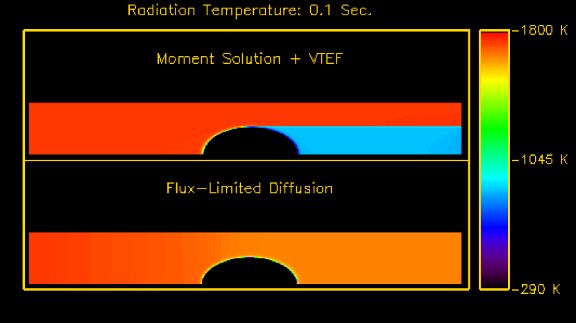
Figure 9: VTEF vs. FLD: the radiation energy density at 0.1 seconds ($3\times 10^{9}$ light-crossing times) for the VTEF calculation (top) and the FLD calculation (bottom). Note that the VTEF calculation has remained essentially unchanged from its asymptotic state in figure 7.

As defined, this problem was evolved for 0.1 seconds, which is $3\times 10^{9}$ light-crossing times for the cylinder. Figures 6 through 8 present images of the radiation temperature distribution throughout the domain during the first ten light-crossing times of the simulation. Figure 6 gives results for a simulation in which the radiation moment variables and the transfer solution were evolved on a 280x80 (ZxR) grid. The PSTAT algorithm was used to compute Eddington tensors; 33 $\mu$ angle cosines were distributed over 16 CPU’s, with three angles stored on the root process and two angles on each of the remaining processes. Four panels showing the full ZxR domain are shown, corresponding to 0.68, 1.0, 2.0, and 10 light-crossing times. To begin with, we see the advance of the broad radiation wave, and the definition of a shadow region as the wave passes over the spheroidal target. As the source becomes fully illuminated, the shadow remains clearly delineated, but there is some leakage of radiation from the illuminated region into the shadow. Because we assume no scattering in the problem, and further because neither the limb of the target nor the low-density gas have yet warmed enough to re-emit significantly, this leakage is not physical. It is due, rather, to the diffusivity of the radiation energy equation which depends upon a “double divergence” of the Eddington tensor (cf. equations (14), (15), and Appendix A). Once the radiation field reaches the state shown in the fourth panel, however, it remains stable with energy leaked into the shadow being transported out the exit boundary. The radiation field at three billion light-crossing times is virtually unchanged from its state at ten light-crossing times (figure 9).

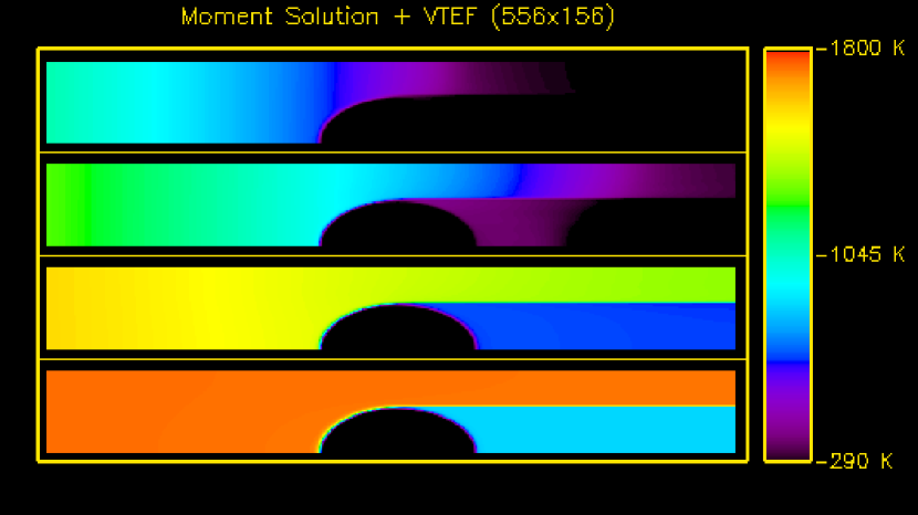
Figure 7: Shadow test with VTEF: as in figure 6, but for a 556x156 moment grid combined with a 280x80 transfer solution grid.

Figure 7 presents the same calculation, assuming the same physics and employing the same transport techniques, for a radiation moment grid at 556x156 resolution. In this run, the moment grid is divided into a 4x4 process topology, and a sampling parameter ($N_{\rm samp}$) of 2 was used to define a CSC grid on which Eddington tensors were computed. Physically, the results are virtually indistinguishable, which shows that the diffusivity in the moment equations is not affected by higher resolution. The root of the problem is not resolution; it is instead a consequence of the fact that fluxes in the radial direction are spuriously generated by a finite-difference stencil that “straddles” boundaries between illuminated and shadowed regions.

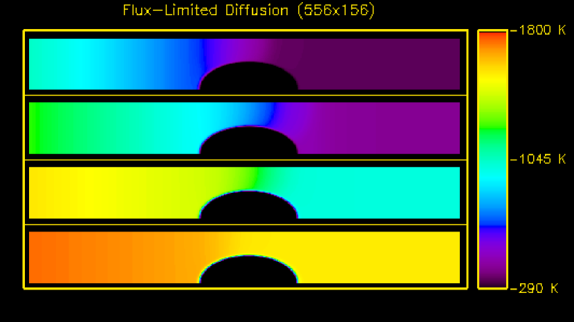
Figure 8: Shadow test with FLD: a flux-limited diffusion comparison test at 556x156 resolution. The times are the same as for the VTEF cases. Note that the cloud shadow is completely destroyed.

While we have identified a significant weakness in the current VTEF implementation, we have not yet moved to remedy it. Instead, we proceed to examine results from the traditional approach to transport: flux-limited diffusion. Figure 8 presents a high-resolution (556x156) run in which the radiation field is evolved according to FLD:

$${\bf F}\ =\ -{c\over\chi}\Lambda(E)\Delta E.$$ (79)

In (79), $\Lambda(E)$ is the flux-limiter; we have used the Levermore-Pomraning limiter for the results given here.

Even after only 10 light-crossing times, the difference between FLD and VTEF is dramatic and fundamental. In the FLD prescription, radiation flows around and surrounds the target as rapidly as it moves down the cylinder. No delineation of a shadow is ever present, and at long times (figure 9) the target is irradiated isotropically, even though the illuminating source is defined to exist at only one end of the cylinder! Thus while we acknowledge room for improvement in the numerical implementation of VTEF, we see already a qualitative difference in the two approaches which will have fundamental consequences when full hydrodynamic simulations are considered. We conclude this section with an examination of figure 10, which shows the variation of radiation temperature with radius at $Z$ = 1.0 cm (the center of the obstructing cloud is at $Z$ = 0.5 cm) at the end of the evolution (0.1 sec). The dashed line indicates the initial profile prior to the passage of the radiation front. Open circles show the radiation temperature computed from a full VTEF calculation; open crosses show results from an FLD calculation. The solid line shows radiation temperatures derived from the zeroth moment of the specific intensity extracted from our transport solver. This is the same quantity used to derive the Eddington tensors for the moment solution, but notice that the radiation energy derived from $I$ does not exhibit the large, spurious leakage of energy into the shadow region. $I$ has risen, within the shadow, above its initial ambient value slightly because of thermal re-emission from low-density gas in the non-shadowed region of the domain. This also contributes (slightly) to the filling in of the shadow in the VTEF case, but there is a large component of this which is artificial. Nonetheless, the VTEF algorithm has managed to preserve a well-defined shadow even after $3\times 10^{9}$ light-crossing times, a task at which FLD fails completely.

6.3 Radiation Hydrodynamics: Radiating Shocks

In our final collection of test results, we marry the radiation transport algorithms to the gas hydrodynamic modules of ZEUS-MP. Our test problem in this instance is the evolution of radiating shock waves in optically thick media. The presence of radiation modifies the shock structure considerably, introducing a radiative precursor which preheats the material downstream from the shock to some characteristic temperature, $T_{-}$. Denoting the temperature behind the shock front as $T_{2}$, we may follow the discussion in Mihalas and Mihalas (1984) and identify two major classes of radiating shocks: subcritical and supercritical shocks. In the subcritical case, $T_{2}$ is greater than $T_{-}$, and the radiation precursor is relatively weak. At higher flow velocities, $T_{-}$increases relative to $T_{2}$, and at some critical velocity $u_{\rm crit}$, the two become equal ($T_{-}$never exceeds $T_{2}$). Shocks for which $u\geq u_{\rm crit}$ are termed supercritical. As shall be seen below, supercritical radiating shocks are characterized by a very large radiation precursor which heats the unshocked material downstream from the shock front.

6.3.1 Subcritical Shocks

Our problem configuration is guided by that published by Ensman (1994), who considered a battery of test problems designed for astrophysical codes. Ensman considered the case of a piston moving through static media, and followed the evolution with a one dimensional, Lagrangean, radiation hydrodynamics code (VISPHOT). Because ZEUS-MP evolves the gas dynamic equations in the Eulerian frame, we pose the problem analogous to the Noh test where a moving medium impacts a stationary reflecting boundary. Velocities in our tests are initialized to match the piston speeds specified in the Ensman paper. Since VISPHOT assumes a spherically symmetric problem, Ensman generated a (nearly) planar problem by placing the medium in a thin shell at large radii. Since our grid is cylindrical, we can produce a rigorously planar shock, and we choose problem dimensions, initial densities, and opacities consistent with those published in Ensman (1994), save for one feature: the Ensman grid attempts to reproduce an infinite plane. Our cylindrical grid has a finite radius which is smaller than the axial length of the domain, which means that our test involves a radiating surface which is formally finite in extent. This effects the degree of forward peaking in the radiation field downstream from the shock, and accounts for some qualitative differences between our profiles and those published by Ensman.

In our subcritical test, we define a cylinder of length $7.0\times 10^{10}$ cm, with an initial uniform density of $7.78\times 10^{-10}$ g ${\rm cm}^{-3}$. The gas and radiation temperatures (initially in equilibrium) were set to 10K at the outer boundary and increased progressively by 0.25K in each interior zone. This choice was made by Ensman to avoid numerical difficulties with zero flux in VISPHOT; we repeat the practice for consistency. This problem assumes a purely absorbing medium with a constant opacity; our value was $3.1\times 10^{-10}$ cm. The physical domain is therefore almost 22 times greater than the photon mean-free path. Thus, while the medium may be characterized as optically thick in toto, individual zones are optically thin, a point we will consider further in the supercritical case.

The problem is initiated by setting the axial velocity equal to $-6.0\times 10^{5}$ cm s^-1 everywhere on the grid. 300 uniform zones were used to span the Z axis, whereas a modest 16 zones spanned the radial direction, itself only $3.2\times 10^{9}$ cm in extent. The domain, then, assumes the shape of a long, narrow pipe, with variations in physical quantities confined to the Z direction.

In order to produce figures which are directly comparable to results obtained with lagrangean codes such as VISPHOT, the “Z” axis shown in the following plots has been transformed to show the positions in a frame in which an unshocked parcel of matter still moving with the inflow velocity, $v_{i}$, is at rest. Thus, if $Z_{i}$ denotes the plot coordinate, and $Z_{o}$ is the lab frame coordinate, we have

$$Z_{i}\ =\ Z_{o}-v_{i}t.$$ (80)

In this way we may represent our results as if they had been generated by a piston in a stationary medium.

Figure 11 shows profiles for the radiation temperature (solid lines) and gas temperature (dashed lines) at 3 fiducial times in the evolution. In this test, the VTEF transport algorithm was not employed. Instead, a constant, isotropic Eddington tensor with values of 1/3 along the diagonal was chosen to close the radiation moment equations. We refer to this choice as the “CTEF” (constant tensor Eddington factor) approximation. In figure 11, the radiation precursor is clearly evident, the matter and radiation temperatures are well out of equilibrium on both sides of the shock front. Figure 12 presents results for the same problem configuration with a full VTEF closure employed in the radiation moment equations. In this case, the PSTAT time-dependent solution to the transfer equation was chosen to calculate the Eddington tensor. The closure values were updated whenever the gas temperature at some point in the domain changed by at least two percent. In this test, we see that the difference between the VTEF and CTEF results is relatively minor. The radiation profiles are slightly broader in the CTEF case, but the positions of the advancing shock front are identical in both cases, as is the matter temperature variation across the shock. This result is perhaps not surprising given that radiation effects are weak in the subcritical case, and the physical domain is optically thick. Furthermore, we note that our solutions are consistent with the subcritical solutions shown in figure 8 of Ensman (1994).

6.3.2 Supercritical Shocks

In the supercritical shock tests, all physical parameters remain the same as in the subcritical case except for the inflow velocity, which has been changed from -6 to -20 km/sec along the Z-axis. As before, the problem is initialized on a 300x16 (ZxR) grid. In plotting profiles of physical quantities at various times, we repeat the practice of transforming Z values into the inertial frame in which the inflowing material is at rest.

In contrast with the subcritical test, we present as our standard result a model in which the full VTEF-PSTAT algorithm is employed. Figure 13 shows profiles in gas and radiation temperature (solid and dashed lines, respectively) for three times in the shock evolution. The radiative precursor has become a dominant feature of the preshock medium.

The significant role played by radiation in the supercritical case suggests that the details of transport physics will be more important than in the subcritical case. We affirm this expectation by presenting a comparison calculation performed with a constant Eddington tensor containing values of 1/3 along the diagonal (our CTEF approximation). Figure 14 combines the gas and radiation temperature profiles from figure 13 with data from the CTEF run. The difference is fairly dramatic, with the CTEF run yielding profiles which are broader but lower in amplitude. The position of the shock front with time is unchanged, as is the relative height and width of the non-equilibrium temperature spike at the shock front. Figure 15 show, for the time at which the middle profile is plotted, the spatial run of the f₁₁ Eddington tensor component. In the vicinity of the shock, high temperatures on both side ensure a relatively isotropic radiation field, but well downstream f₁₁ approaches the streaming limit of 1, even though the medium is (globally) optically thick. Of further interest is the slight dip below 1/3 at the position of the shock front. This is a real effect which is characteristic of a strong transverse component in the specific intensity at that point.

That the results vary strongly between the CTEF and VTEF solutions is a major point of departure between our caculations and the corresponding solutions in figure 15 of Ensman (1994). We remind the reader, however, of a significant geometric difference between the two cases: the Ensman model, being defined on a thin spherical shell at a large radius, approximates a thin plane of infinite extent in the directions perpendicular to the propagation vector. Our calculation, however, is initialized on a long, narrow pipe. The radiating surface we compute is therefore finite and results in a radiation field which becomes very forward-peaked (cf. fig. 15). The analytic value for the scalar Eddington factor located at the surface of an infinite plane is 1/2, which is much closer to an isotropic value than that seen in our calculations. It is therefore not surprising that our supercritical shock tests exhibit a stronger sensitivity to the transport physics than those performed by Ensman. In the subcritical case, in which radiative effects are minor, the details of transport are considerably less important.

Figure 16 shows that, for this problem, the specific choice by which variable Eddington tensors are computed is less important than the decision to allow them to vary at all. Because this problem is optically thick, the radiation field changes on time scales which are long compared to the light-crossing time (roughly 2 seconds). Thus there is very little gained by using either time-dependent form of the VTEF solution (TRET or PSTAT) in place of a purely static solution. We note, however, that this statement would not hold were one to model a medium marked by a transition from optically thick to thin media, such as a stellar surface (in the case of photon transport) or the iron core of a collapsing supernova progenitor (in the case of neutrino transport).

7 Summary and Discussion

In this paper, we have presented a new code for performing RHD simulations on parallel computers. The algorithms discussed here include and augment the functionality of the serial algorithms documented in Stone et. al (1992). We have documented both the analytic and discrete forms of the radiation moment solution and the Eddington tensor closure term. We have described three different methods for computing a short-characteristic formal solution to the transfer equation, from which our VTEF closure term is derived. Two of these techniques include time dependence, a feature not typically associated with the formal solution in astrophysics literature. Two key numerical components of our implementation have been highlighted: the biconjugate gradient linear system solver, written for general use on massively parallel computers, and our techniques for parallelizing both the radiation moment solution and the transfer solution. Finally, we have presented a suite of test problems which run the gamut from optically thin transport with a fixed Eddington tensor, to full RHD+VTEF calculations of radiating shocks.

This document and our code possess a number of features which are new with respect to Paper III and the serial code described therein. In the moment equations, we chose to accompany the radiation energy equation with an equation for the gas energy rather than adopting a total energy equation. This choice allows us to employ a different matter-radiation coupling scheme with three very attractive features: (1) it is particularly robust in regimes where matter and radiation are far out of equilibrium, (2) it allows the construction of a moment solution matrix involving only one dependent field variable, and (3) it is extremely well-suited to implementation on parallel platforms. In the transfer solution, we have retained the original static method, suitable for computing Eddington tensors for static or quasistatic radiation fields, but we have added two algorithms which include time dependence in different ways. One of these treats temporal effects by time-retarding the opacities and source functions encountered along a characteristic ray. The second of these, which we have adopted as our default method for problems needing a time-dependent treatment, builds a discrete form of the time derivative operator directly into the characteristic solution. This “pseudostatic” form has an advantage over the “time-retarded” form in that it is not necessary to save opacities and emissivities from a previous timestep. All three algorithms may be used to compute Eddington tensors on the full moment solution grid, or upon a subset of mesh points obtained by subsampling the moment grid at regular intervals along both coordinates.

Design for parallel execution is an entirely new feature with respect to the older code. We have used the Message-Passing Interface (MPI) standard exclusively in constructing our code for parallel use. In the gas dynamical and radiation moment solution modules, we have distributed work among parallel processors via spatial domain decomposition. In contrast, the transfer solution has been subdivided over the $\mu$ angle coordinate, owing to the spatially recursive nature of the SC solution.

This work also contains a more diverse set of test problems than that provided in Paper III. We feel that this is particularly important, because the RHD modules in Paper III have remained unused since they were written more than ten years ago, due in part to the subsequent research pursuits of their creator, and also to the fact that the publicly available version of ZEUS-2D contained an FLD module rather than the VTEF algorithm described in Paper III. As a result, the viability of this VTEF approach for multidimensional calculations has not been properly documented in the astrophysical literature. As a first step toward correcting this shortfall, we have provided full RHD tests to which the serial algorithm was never subjected. In addition, we have focused considerable attention on multidimensional radiation fields containing a shadowed region, consistent both the original mission of this LLNL-funded project and with anticipated astrophysics applications to come.

The test problems we have examined allow us to consider the strengths and weaknesses of the VTEF method for multi-dimensional problems. The major weaknesses of the method, as currently implemented, are the diffusivity of the discrete moment equations and limitations upon the extent to which the transport solution can track rapid time variation of the radiation field. The diffusivity of the moment solution is a direct consequence of the difference stencil used to discretize the moment equations; the “double divergence” term in the radiation energy equation (see equations 29 and 30) results in finite differences which artificially connect regions in space on either side of physical boundaries in the radiation field, such as the shadow edges in our illuminated cloud problem. In our test case, this prevents the VTEF algorithm from reproducing such shadowed regions as fully as we would like. Nonetheless, a noticeable shadow is maintained for very long timescales, with leakage of energy (via the R-component of the flux) into the shadowed region balanced by transmission (via the Z-component of the flux) of energy through the exit boundary.

The second problem affects the degree of consistency between the moment solution and transport solution for the radiation field. Mathematically, our radiation moment equation results from a zeroth angular moment of the time-dependent equation of transfer; using a VTEF closure for the moment equation is therefore accurate only if the radiation solutions as characterized by these two equations are mathematically consistent. An equivalent statement is that the radiation energy density produced from the moment equation should equal that obtained through a direct integration of the specific intensity over all solid angles. The first test problem in §6 shows that our moment solution is capable of following a sharply defined radiation front when the Eddington tensor is an idealized constant with ${\bf f}_{11}$ = 1. Our formal solution, however, includes time dependence in an approximate manner, and disagrees strongly with the moment solution when the radiation field shows a rapid variation in time (and therefore space).

We illustrate this behavior with comparing two streaming problems computed with the full VTEF method. The physical characteristics of the two cases are identical and are taken from the cloud problem, albeit with the dense cloud removed in favor of a uniform medium. As with the cloud test, the illuminating source intensity increases with a prescribed e-folding time. In the case shown in figure  17, the e-folding time is equal to the light-crossing time along the Z-axis; in figure 18 this value has been decreased by an order of magnitude. In both graphs we have plotted the radiation temperature derived from the moment solution for the radiation energy density, and compared it to that derived from an angular integration of the specific intensity. When the radiation source is illuminated slowly, we see close agreement at all times between the two solutions. When the radiation source is illuminated rapidly, there is a clear disagreement between the two. In particular, the profiles computed from the transport solver begin to “lead,” to a significant degree, those from the moment solution as the wavefront progresses. The significance of this becomes apparent when we realize that the Eddington tensor deviates from isotropy everywhere that the specific intensity has risen from its ambient value. Once the Eddington tensor changes from its isotropic value, the divergence terms in the flux equation become non-zero and generate flux. This means that fluxes from the moment solution at a given point in space will become non-zero even before the radiation front has overrun that point, clearly a non-physical result.

As applied to the cloud problem, the consequences of these two shortcomings are: (1) flux in the R-direction will leak radiation into the shadowed region artificially, and (2) this behavior will occur even before the radiation front has swept over the cloud, if the radiation source is illuminated too rapidly. As a practical matter, this test problem needed to be designed with some care; attempting to illuminate the source too quickly led to unrecoverable errors in the radiation field evolution. While there are phenomena in astrophysics in which light-travel times may matter (e.g. the emergence of radiation fronts from optically thick surfaces), problems abound in which the radiation field may be treated as time independent, or at worst quasistatic. In this instance, our equations show good internal consistency, and the dangers of pathological behavior are greatly reduced. Further, we note that considerable overall improvement to the method will be obtained if our discrete solution is redesigned to eliminate (or greatly reduce) the spurious generation of fluxes at interface boundaries. This problem is not unique to our method, and alternative schemes for tensor diffusion problems have been published in the radiation transport literature (Morel et. al, 1998, 2001). With the support of the Department of Energy, we are now undertaking to implement our VTEF equations with a higher-order spatial scheme which satisfies the appropriate flux constraints. Results of this effort will be reported in future work.

The strengths of our method, in our view, are threefold. With regard to angular variations in the radiation intensity, the difference between the VTEF and FLD solutions is fundamental and dramatic. While the VTEF solution shows room for quantitative improvement, the qualitative behavior is physically sensible, while that of the FLD solution is not. This result alone compels us to pursue the VTEF approach further, with an eye toward relieving the diffusivity issues identified above. This algorithm is also particularly suited to environments where matter and radiation are out of equilibrium, a situation often encountered in strongly dynamic environments. The numerical scheme used to implement matter radiation coupling has the further advantage of allowing an implicit linear system solve for the radiation energy density alone, in contrast to the two-variable coupled system documented in Paper III. Finally, we note that our method is suited for large problems distributed across parallel architectures. This statement is even truer for problems which require only a static transfer solution for Eddington tensors (owing to a far lower memory requirement), or, in the most favorable case, problems in which static Eddington tensors can be computed analytically. In this instance, the brunt of the computational burden lies in the linear system solve for $E_{rad}$, and is thus on the same order of the cost for an analogous solution for FLD. We therefore view this method as a topic worthy of continued study, with regard to both algorithm development and astrophysical applications.

Appendix A The Radiation Moment Equation Linear System Matrix

Equation (41), when written on a discrete mesh, leads to a linear system for a solution vector consisting of the discrete values of $E$ (the $E_{i,j}$) everywhere on the moment solution grid. This matrix equation is represented schematically by equation (43), which shows that our system involves a nine-band system. The central $E$ value on the stencil ($E_{i,j}$) is coupled to $E_{i-1,j}$ and $E_{i+1,j}$ via the first subdiagonal ($DM1_{i,j}$) and superdiagonal ($DP1_{i,j}$), respectively. Subdiagonals $DM4_{i,j}$, $DM3_{i,j}$, and $DM2_{i,j}$ couple solution elements $E_{i-1,j-1}$, $E_{i,j-1}$, and $E_{i+1,j-1}$, respectively, and superdiagonals $DP2_{i,j}$, $DP3_{i,j}$, and $DP4_{i,j}$ couple elements $E_{i-1,j+1}$, $E_{i,j+1}$, and $E_{i+1,j+1}$.

Refering to equation (41), we note that all three terms on the LHS of (41) contribute to $D00_{i,j}$, but only the second term of (41) produces off-diagonal matrix elements. The third term of (41) produces no off-diagonal elements because it is viewed as product of the central $E_{i,j}$ and the quantity $\nabla{\bf v}:{\bf f}$, where it is assumed that $\nabla{\bf v}$ and ${\bf f}$ are already known. Refering to the definitions in § 2.3, we may therefore write for the main diagonal:

$$D00_{i,j}\ =\ \left(1+{k_{2}(i,j)\over\Phi(i,j)}\right)\ +\ \Delta t(\nabla{\bf v}:{\bf f})_{i,j}\ +\ T2_{00}(i,j),$$ (A1)

where $T2_{00}(i,j)$ are the contributions to $D00_{i,j}$ from the discretized second term in (41). The form of $\nabla{\bf v}:{\bf f}$ has been documented in Paper III (albeit with ${\bf f}$ replaced by ${\bf P}$), and will not be reproduced here. The remaining pieces of $D00_{i,j}$ and all of the off-diagonal bands are generated by the discrete form of $T2$, which we will now document.

There are four steps to this documentation process. The first step is to properly express the required components of the tensor divergence term, assuming 2-D cylindrical symmetry. Considering our radiation stress tensor, ${\bf P}$, the symmetry assumption implies that ${\bf P}_{12}$, ${\bf P}_{21}$, ${\bf P}_{13}$, ${\bf P}_{31}$, ${\bf P}_{23}$, and ${\bf P}_{32}$ are all zero. Regardless of symmetry, it is also true that the trace of ${\bf P}$ is an invariant, and is identically equal to $E$. This allows us to write further that

$${\bf P}_{33}\ =\ E-{\bf P}_{11}-{\bf P}_{22},$$ (A2)

or alternatively,

$${\bf f}_{33}\ =\ 1-{\bf f}_{11}-{\bf f}_{22},$$ (A3)

This relation was incorrectly expressed in the derivation of the divergence terms documented in Paper III.

Making use of the general expressions in Stone and Norman (1992a) for a tensor divergence, and applying our conditions of symmetry and trace invarience, we may write:

$$\left({\bf\nabla\cdot{\bf P}}\right)^{(1)}\ =\ {1\over g2g31}{\partial\over\partial x_{1}}\left(g_{2}g_{31}{\bf P}_{11}\right)\ +\ {1\over g_{2}}{\partial\over\partial V_{2}}\left(g_{32}{\bf P}_{12}\right),$$ (A4)

and

$$\left({\bf\nabla\cdot{\bf P}}\right)^{(2)}\ =\ g_{2}{\partial\over\partial V_{1}}\left(g_{31}{\bf P}_{12}\right)\ +\ {1\over g_{2}}{\partial\over\partial V_{2}}\left(g_{32}{\bf P}_{22}\right)\ -\ {\left(E-{\bf P}_{11}-{\bf P}_{22}\right)\over g_{2}g_{32}}{\partial g_{32}\over\partial x_{2}}.$$ (A5)

Step two of derivation is to employ the relation ${\bf P}={\bf f}E$ and discretize the tensor divergence terms, employing the same finite difference conventions used in the ZEUS-2D code:

$$\left({\bf\nabla\cdot{\bf P}}\right)^{(1)}_{i,j} \rightarrow {1\over{\rm g2a_{i}}~{}{\rm g31a_{i}}}\left[{{{\rm g2b_{i}g31b_{i}}{\bf f}11_{i,j}E_{i,j}\ -\ {\rm g2b_{i-1}g31b_{i-1}}{\bf f}11_{i-1,j}E_{i-1,j}}\over{\rm dx1b_{i}}}\right]$$ (A6)

$$+ {{\rm g32a_{j+1}}{\bf f}12_{i,j+1}\langle E\rangle_{i,j+1}\ -\ {\rm g32a_{j}}{\bf f}12_{i,j}\langle E\rangle_{i,j}\over{\rm g2a_{i}~{}dvl2a_{j}}};$$

$$\left({\bf\nabla\cdot{\bf P}}\right)^{(2)}_{i,j} \rightarrow \left[{{\rm g32b_{j}}{\bf f}22_{i,j}E_{i,j}\ -\ {\rm g32b_{j-1}}{\bf f}22_{i,j-1}E_{i,j-1}}\over{\rm g2b_{i}~{}dvl2b_{j}}\right]$$ (A7)

$$+ \left({\rm g2b_{i}}\over{\rm dvl1a_{i}}\right)\left({\rm g31a_{i+1}}{\bf f}12_{i+1,j}\langle E\rangle_{i+1,j}\ -\ {\rm g31a_{i}}{\bf f}12_{i,j}\langle E\rangle_{i,j}\right)$$

$$- \left(1\over 2\right)\left(1\over{\rm g2b_{i}~{}g32a_{j}}\right)\left(\partial{\rm g32a}_{j}\over\partial{\rm x2}\right)\times$$

$$\left[E_{i,j}\left(1-{\bf f}11_{i,j}-f22_{i,j}\right)+E_{i,j-1}1\left(1-{\bf f}11_{i,j-1}1-f22_{i,j-1}1\right)\right]$$

In (A6) and (A7), $\langle E\rangle$ signifies an average value of $E$ at the vertex of four neighboring zones; i.e.

$$\langle E\rangle_{i,j}\ =\ {1\over 4}\left(E_{i,j}\ +\ E_{i-1,j}\ +\ E_{i,j-1}\ +\ E_{i-1,j-1}\right)$$ (A8)

In step three, we write a discrete form of the ${\bf\nabla}\cdot({\bf b}{\bf\nabla\cdot{\bf P}})$, where b is given by

$${\bf b}\ =\ {c^{2}\Delta t\over\left(1+c\Delta t\chi_{\bf F}\right)}$$ (A9)

b is written in boldface to indicate that it is dependent upon the component of ${\bf\nabla\cdot{\bf P}}$ under consideration, owing to the variation (in the general case) of $\chi_{\bf F}$ with direction. Employing our usual standard for writing vector divergences, we may write

$${\bf\nabla}\cdot({\bf b}{\bf\nabla\cdot{\bf P}}) \rightarrow {{\rm g2a_{i+1}g31a_{i+1}b^{(1)}_{i+1,j}}({\bf\nabla\cdot{\bf P}})_{i+1,j}^{(1)}\ -\ {\rm g2a_{i}g31a_{i}b^{(1)}_{i,j}}({\bf\nabla\cdot{\bf P}})_{i,j}^{(1)}\over{\rm dvl1a_{i}}}$$ (A10)

$$+ {{\rm g32a_{j+1}b^{(2)}_{i,j+1}}({\bf\nabla\cdot{\bf P}})_{i+1,j}^{(2)}\ -\ {\rm g32a_{j}b^{(2)}_{i,j}}({\bf\nabla\cdot{\bf P}})_{i,j}^{(2)}\over{\rm g2b_{i}~{}dvl2a_{j}}}$$

The final step in the derivation of the matrix elements is the substitution of expressions (A6) and (A7) into (A10). All terms contributing to the main diagonal, for example, are coefficients of the various terms containing $E_{i,j}$. Expressions for each of the sub- and superdiagonals are found by collecting the coefficients of the appropriate discrete $E$ element within the nine-point stencil. We will not reproduce this algebra here, but we document the final result. Because the expressions are complicated, we will subdivide result for each matrix band in a manner reflective of the Fortran expressions used in the code. We write:

$$DM4_{i,j} = C2_{i,j}\cdot{\rm b^{(1)}}_{i}\cdot{\rm dp1}_{i-1,j-1}\ +\ C4_{i,j}\cdot{\rm b^{(2)}}_{j}\cdot{\rm dp2}_{i-1,j-1};$$ (A11a)

$$DM3_{i,j} = C1_{i,j}\cdot{\rm b^{(1)}}_{i+1}\cdot{\rm dp1p}_{i,j-1}\ +\ C2_{i,j}\cdot{\rm b^{(1)}}_{i}\cdot{\rm dp1}_{i,j-1}$$ (A11b)

$$+ C4_{i,j}\cdot{\rm b^{(2)}}_{j}\cdot{\rm dp2}_{i,j-1};$$

$$DM2_{i,j} = C1_{i,j}\cdot{\rm b^{(1)}}_{i+1}\cdot{\rm dp1p}_{i+1,j-1}\ +\ C4_{i,j}\cdot{\rm b^{(2)}}_{j}\cdot{\rm dp2}_{i+1,j-1};$$ (A11c)

$$DM1_{i,j} = C2_{i,j}\cdot{\rm b^{(1)}}_{i}\cdot{\rm dp1}_{i-1,j}\ +\ C3_{i,j}\cdot{\rm b^{(2)}}_{j+1}\cdot{\rm dp2p}_{i-1,j}$$ (A11d)

$$+ C4_{i,j}\cdot{\rm b^{(2)}}_{j}\cdot{\rm dp2}_{i-1,j};$$

$$D00_{i,j} = C1_{i,j}\cdot{\rm b^{(1)}}_{i+1}\cdot{\rm dp1p}_{i,j}\ +\ C2_{i,j}\cdot{\rm b^{(1)}}_{i}\cdot{\rm dp1}_{i,j}$$ (A11e)

$$+ C3_{i,j}\cdot{\rm b^{(2)}}_{j+1}\cdot{\rm dp2p}_{i,j}\ +\ C4_{i,j}\cdot{\rm b^{(2)}}_{j}\cdot{\rm dp2}_{i,j};$$

$$DP1_{i,j} = C1_{i,j}\cdot{\rm b^{(1)}}_{i+1}\cdot{\rm dp1p}_{i+1,j}\ +\ C3_{i,j}\cdot{\rm b^{(2)}}_{j+1}\cdot{\rm dp2p}_{i+1,j}$$ (A11f)

$$+ C4_{i,j}\cdot{\rm b^{(2)}}_{j}\cdot{\rm dp2}_{i+1,j};$$

$$DP2_{i,j} = C2_{i,j}\cdot{\rm b^{(1)}}_{i}\cdot{\rm dp1}_{i-1,j+1}\ +\ C3_{i,j}\cdot{\rm b^{(2)}}_{j+1}\cdot{\rm dp2p}_{i-1,j+1};$$ (A11g)

$$DP3_{i,j} = C1_{i,j}\cdot{\rm b^{(1)}}_{i+1}\cdot{\rm dp1p}_{i,j+1}\ +\ C2_{i,j}\cdot{\rm b^{(1)}}_{i}\cdot{\rm dp1}_{i,j+1}$$ (A11h)

$$+ C3_{i,j}\cdot{\rm b^{(2)}}_{j+1}\cdot{\rm dp2p}_{i,j+1};$$

$$DP4_{i,j} = C1_{i,j}\cdot{\rm b^{(1)}}_{i+1}\cdot{\rm dp1p}_{i+1,j+1}\ +\ C3_{i,j}\cdot{\rm b^{(2)}}_{j+1}\cdot{\rm dp2p}_{i+1,j+1};$$ (A11i)

where

$$C1_{i,j} = -\Delta t{{\rm g2a_{i+1}}~{}{\rm g31a_{i+1}}\over{\rm dvl1a_{i}}};$$ (A12)

$$C2_{i,j} = \ \ \Delta t{{\rm g2a_{i}}~{}{\rm g31a_{i}}\over{\rm dvl1a_{i}}};$$ (A13)

$$C3_{i,j} = -\Delta t{{\rm g32a_{j+1}}\over{\rm g2b_{i}}~{}{\rm dvl2a_{j}}};$$ (A14)

$$C4_{i,j} = \ \ \Delta t{{\rm g32a_{j}}\over{\rm g2b_{i}}~{}{\rm dvl2a_{j}}}.$$ (A15)

In (A11), “dp1” is shorthand for the coefficients of a particular element of $E$ in the expression for $({\bf\nabla\cdot{\bf P}})_{i,j}^{(1)}$. The element of $E$ in question is indicated by the subscripts on dp1. There are analogous relationships between “dp1p” and $({\bf\nabla\cdot{\bf P}})_{i+1,j}^{(1)}$, “dp2” and $({\bf\nabla\cdot{\bf P}})_{i,j}^{(2)}$, and “dp2p” and $({\bf\nabla\cdot{\bf P}})_{i,j+1}^{(2)}$. Save for modifications due to applied boundary conditions, we complete our documentation of the matrix elements by listing the values for the four “dp$\{n\}$” quantities at the required $E$ index values. For $({\bf\nabla\cdot{\bf P}})^{(1)}$ at $(i,j)$, we have:

$${\rm dp1}_{i-1,j-1} = -\left(1\over 4\right){{\rm g32a}_{j}{\bf f}12_{i,j}\over{\rm g2a}_{i}~{}{\rm dvl2a}_{j}};$$ (A16)

$${\rm dp1}_{i,j-1} = -\left(1\over 4\right){{\rm g32a}_{j}{\bf f}12_{i,j}\over{\rm g2a}_{i}~{}{\rm dvl2a}_{j}};$$ (A17)

$${\rm dp1}_{i-1,j} = -{{\rm g2b}_{i-1}{\rm g31b}_{i-1}{\bf f}11_{i-1,j}\over{\rm g2a}_{i}~{}{\rm g31a}_{i}~{}{\rm dx1b}_{i}}$$ (A18)

$$+ \left(1\over 4\right){{{\rm g32a}_{j+1}{\bf f}12_{i,j+1}\ -\ {\rm g32a}_{j}{\bf f}12_{i,j}}\over{\rm g2a}_{i}~{}{\rm dvl2a}_{j}};$$

$${\rm dp1}_{i,j} = {{\rm g2b}_{i}{\rm g31b}_{i}{\bf f}11_{i,j}\over{\rm g2a}_{i}~{}{\rm g31a}_{i}~{}{\rm dx1b}_{i}}\ +\ \left(1\over 4\right){{{\rm g32a}_{j+1}{\bf f}12_{i,j+1}\ -\ {\rm g32a}_{j}{\bf f}12_{i,j}}\over{\rm g2a}_{i}~{}{\rm dvl2a}_{j}};$$ (A19)

$${\rm dp1}_{i-1,j+1} = \left(1\over 4\right){{\rm g32a}_{j+1}{\bf f}12_{i,j+1}\over{\rm g2a}_{i}~{}{\rm dvl2a}_{j}};$$ (A20)

$${\rm dp1}_{i,j+1} = \left(1\over 4\right){{\rm g32a}_{j+1}{\bf f}12_{i,j+1}\over{\rm g2a}_{i}~{}{\rm dvl2a}_{j}}.$$ (A21)

For $({\bf\nabla\cdot{\bf P}})^{(1)}$ at $(i+1,j)$, we have:

$${\rm dp1p}_{i,j-1} = -\left(1\over 4\right){{\rm g32a}_{j}{\bf f}12_{i+1,j}\over{\rm g2a}_{i+1}~{}{\rm dvl2a}_{j}};$$ (A22)

$${\rm dp1p}_{i+1,j-1} = -\left(1\over 4\right){{\rm g32a}_{j}{\bf f}12_{i+1,j}\over{\rm g2a}_{i+1}~{}{\rm dvl2a}_{j}};$$ (A23)

$${\rm dp1p}_{i,j} = -{{\rm g2b}_{i}{\rm g31b}_{i}{\bf f}11_{i,j}\over{\rm g2a}_{i+1}~{}{\rm g31a}_{i+1}~{}{\rm dx1b}_{i+1}}$$ (A24)

$$+ \left(1\over 4\right){{{\rm g32a}_{j+1}{\bf f}12_{i+1,j+1}\ -\ {\rm g32a}_{j}{\bf f}12_{i+1,j}}\over{\rm g2a}_{i+1}~{}{\rm dvl2a}_{j}};$$

$${\rm dp1p}_{i+1,j} = {{\rm g2b}_{i+1}{\rm g31b}_{i}{\bf f}11_{i+1,j}\over{\rm g2a}_{i+1}~{}{\rm g31a}_{i+1}~{}{\rm dx1b}_{i+1}}$$ (A25)

$$+ \left(1\over 4\right){{{\rm g32a}_{j+1}{\bf f}12_{i+1,j+1}\ -\ {\rm g32a}_{j}{\bf f}12_{i+1,j}}\over{\rm g2a}_{i+1}~{}{\rm dvl2a}_{j}};$$

$${\rm dp1p}_{i,j+1} = \left(1\over 4\right){{\rm g32a}_{j+1}{\bf f}12_{i+1,j+1}\over{\rm g2a}_{i+1}~{}{\rm dvl2a}_{j}};$$ (A26)

$${\rm dp1p}_{i+1,j+1} = \left(1\over 4\right){{\rm g32a}_{j+1}{\bf f}12_{i+1,j+1}\over{\rm g2a}_{i+1}~{}{\rm dvl2a}_{j}}.$$ (A27)

For $({\bf\nabla\cdot{\bf P}})^{(2)}$ at $(i,j)$, we have:

$${\rm dp2}_{i-1,j-1}\ =\ -\left(1\over 4\right){{\rm g2b}_{i}{\rm g31a}_{i}{\bf f}12_{i,j}\over{\rm dvl1a}_{i}};$$ (A28)

$${\rm dp2}_{i,j-1} = -{{\rm g32b}_{j-1}{\bf f}22_{i,j-1}\over{\rm g2b}_{i}~{}{\rm dvl2b}_{j}}\ -\ \left(1\over 2\right){1\over{\rm g2b}_{i}~{}{\rm g32a}_{j}}{\partial{\rm g32a}_{j}\over\partial{\rm x2}}\left(1-{\bf f}11_{i,j-1}-{\bf f}22_{i,j-1}\right)$$ (A29)

$$+ \left(1\over 4\right){{\rm g2b}_{i}\over{\rm dvl1a}_{i}}\left({\rm g31a}_{i+1}{\bf f}12_{i+1,j}\ -\ {\rm g31a}_{i}{\bf f}12_{i,j}\right);$$

$${\rm dp2}_{i+1,j-1} = \left(1\over 4\right){{\rm g2b}_{i}{\rm g31a}_{i+1}{\bf f}12_{i+1,j}\over{\rm dvl1a}_{i}};$$ (A30)

$${\rm dp2}_{i-1,j} = -\left(1\over 4\right){{\rm g2b}_{i}{\rm g31a}_{i}{\bf f}12_{i,j}\over{\rm dvl1a}_{i}};$$ (A31)

$${\rm dp2}_{i,j} = {{\rm g32b}_{j}{\bf f}22_{i,j}\over{\rm g2b}_{i}~{}{\rm dvl2b}_{j}}\ -\ \left(1\over 2\right){1\over{\rm g2b}_{i}~{}{\rm g32a}_{j}}{\partial{\rm g32a}_{j}\over\partial{\rm x2}}\left(1-{\bf f}11_{i,j}-{\bf f}22_{i,j}\right)$$ (A32)

$$+ \left(1\over 4\right){{\rm g2b}_{i}\over{\rm dvl1a}_{i}}\left({\rm g31a}_{i+1}{\bf f}12_{i+1,j}\ -\ {\rm g31a}_{i}{\bf f}12_{i,j}\right);$$

$${\rm dp2}_{i+1,j}\ =\ \left(1\over 4\right){{\rm g2b}_{i}{\rm g31a}_{i+1}{\bf f}12_{i+1,j}\over{\rm dvl1a}_{i}}.$$ (A33)

For $({\bf\nabla\cdot{\bf P}})^{(2)}$ at $(i,j+1)$, we have:

$${\rm dp2p}_{i-1,j}\ =\ -\left(1\over 4\right){{\rm g2b}_{i}{\rm g31a}_{i}{\bf f}12_{i,j}\over{\rm dvl1a}_{i}};$$ (A34)

$${\rm dp2p}_{i,j} = -{{\rm g32b}_{j}{\bf f}22_{i,j}\over{\rm g2b}_{i}~{}{\rm dvl2b}_{j+1}}\ -\ \left(1\over 2\right){1\over{\rm g2b}_{i}~{}{\rm g32a}_{j+1}}{\partial{\rm g32a}_{j+1}\over\partial{\rm x2}}\left(1-{\bf f}11_{i,j}-{\bf f}22_{i,j}\right)$$ (A35)

$$+ \left(1\over 4\right){{\rm g2b}_{i}\over{\rm dvl1a}_{i}}\left({\rm g31a}_{i+1}{\bf f}12_{i+1,j+1}\ -\ {\rm g31a}_{i}{\bf f}12_{i,j+1}\right);$$

$${\rm dp2p}_{i+1,j} = \left(1\over 4\right){{\rm g2b}_{i}{\rm g31a}_{i+1}{\bf f}12_{i+1,j+1}\over{\rm dvl1a}_{i}};$$ (A36)

$${\rm dp2p}_{i-1,j+1} = -\left(1\over 4\right){{\rm g2b}_{i}{\rm g31a}_{i}{\bf f}12_{i,j+1}\over{\rm dvl1a}_{i}};$$ (A37)

$${\rm dp2p}_{i,j+1} = {{\rm g32b}_{j+1}{\bf f}22_{i,j+1}\over{\rm g2b}_{i}~{}{\rm dvl2b}_{j+1}}\ -\ \left(1\over 2\right){1\over{\rm g2b}_{i}~{}{\rm g32a}_{j+1}}{\partial{\rm g32a}_{j+1}\over\partial{\rm x2}}\left(1-{\bf f}11_{i,j+1}-{\bf f}22_{i,j+1}\right)$$ (A38)

$$+ \left(1\over 4\right){{\rm g2b}_{i}\over{\rm dvl1a}_{i}}\left({\rm g31a}_{i+1}{\bf f}12_{i+1,j+1}\ -\ {\rm g31a}_{i}{\bf f}12_{i,j+1}\right);$$

$${\rm dp2p}_{i+1,j+1} = \left(1\over 4\right){{\rm g2b}_{i}{\rm g31a}_{i+1}{\bf f}12_{i+1,j+1}\over{\rm dvl1a}_{i}}.$$ (A39)

Figure 1: The distribution of coarse-grid points, used for the CSC transfer solution, relative to the full-resolution moment solution grid. The case of $N_{\rm samp}$ = 2 is shown. The fine grid is shown by the small dots; the open squares indicate the mesh points selected for the transfer solution. In the case of a spatially parallelized calculation, this pattern is replicated on the local subgrid contained on each processor.

Figure 2: An example of the data movement tree structure for a global sum operation among eight processors. Operations begin at the top level, with neighboring pairs of rank (n-1,n) combining data on processor (n-1). The process proceeds down each level until the root processor (0) has collected all the data. At a given level, the data movement within all processor pairs proceeds in parallel.

Figure 3: Optically-thin streaming with a step-function source: hyperbolic moment solution.

Figure 4: Optically-thin streaming with a time-rounded source: hyperbolic moment solution.

Figure 5: Non-linear Marshak wave: Numerical solutions (curves) and analytic solutions (circles/squares)

Figure 6: Shadow test with VTEF: the passage of a plane wave over an opaque spheriod. From top to bottom, the panels correspond to 0.68, 1, 2, and 10 light-crossing times. The moment variables and Eddington tensors were both computed on a 280x80 (ZxR) grid.

Figure 10: Radial profiles of radiation temperature: computed values of T_rad from FLD (crosses) and VTEF (open circles), compared to that derived by integrating the specific intensity over angle (solid line). The temperature at t = 0 is indicated by the dashed line.

Figure 11: Subcritical Shocks: gas (solid line) and radiation (dashed line) temperatures at $1.7\times 10^{4}$, $2.8\times 10^{4}$, and $3.8\times 10^{4}$ seconds.

Figure 12: Subcritical Shocks: Temperature profiles computed with VTEF-PSTAT algorithm (curves), compared to those computed assuming a constant, isotropic Eddington tensor (circles and squares). The times are the same as those in figure 11.

Figure 13: Supercritical Shocks: gas (solid line) and radiation (dashed line) temperatures at $4.0\times 10^{3}$, $7.5\times 10^{3}$, and $1.3\times 10^{4}$ seconds.

Figure 14: Supercritical Shocks: Temperature profiles computed with the VTEF-PSTAT algorithm (curves), compared to those computed assuming a constant, isotropic Eddington tensor (circles and squares). The times are the same as those in figure 13.

Figure 15: Supercritical Shocks: The f₁₁ Eddington tensor component, at t = $7.5\times 10^{3}$ seconds, for the run shown in figure 13. The dashed line is located at a value of 1/3. Note the dip below 1/3 at the position of the shock front, a known signature of radiating shocks.

Figure 16: Supercritical Shocks: A comparison of gas temperature profiles resulting from all four Eddington factor calculations.

Figure 17: Radiation temperatures from the moment solution (solid line) compared to those from the transfer solution (dashed line) for the case of a slowly varying illuminating source incident on a uniform medium.

Figure 18: As in figure 17, but for a rapidly varying radiation source.

References

- Adams (1997) Adams, M. L. 1997, Trans. Theory and Stat. Phys., 26(4&5), 385
- Baldwin et. al (1999) Baldwin, C., Brown, P., Falgout, R., Graziani, F., & Jones, J. 1999, J. Chem. Phys., 154, 1
- Barret et. al (1994) Barret, R., Berry, M., Chan, T., Demmel, J., Donato, J., Dongarra, J., Eijkhout, V., Pozo, R., Romine, C., & Van der Vorst, H. 1994, Templates for the Solution of Linear Systems: Building Blocks for Iterative Methods, Philadelphia: SIAM 1994
- Ensman (1994) Ensman, L., 1994, ApJ, 424, 275
-
Fiedler (1997)
Fiedler, R. A. 1997, Optimization
and Scaling of Shared-Memory and Message-Passing Implementations of the
ZEUS Hydrodynamics Algorithm,
http://www.supercomp.org/sc97/proceedings/TECH/FIEDLER/INDEX.HTM - Foster (1995) Foster, I. 1995, Designing and Building Parallel Programs, Addison-Wesley, 1995
- Mihalas and Auer (1999) Mihalas, D. M., & Auer, L. H. 1999, Los Alamos National Laboratory Technical Report #LA-UR-99-6018
- Mihalas and Mihalas (1984) Mihalas, D. M., & Mihalas, B. W. 1984, Foundations of Radiation Hydrodynamics, Oxford: Oxford University Press, 1984
- Mihalas and Weaver (1982) Mihalas, D. M., & Weaver, R. A. 1982, J. Quant. Spec. Radiat. Transf., 28, 213
- Morel et. al (1998) Morel, J. E., Roberts, R. M., & Shashkov, M. J. 1998, J. Chem. Phys., 144, 17
- Morel et. al (2001) Morel, J. E., Hall, M. L., & Shashkov, M. J. 2001, J. Chem. Phys., 170, 338
- Pomraning (1979) Pomraning. G. C. 1979, J. Quant. Spec. Radiat. Transf., 21, 249
- Stone and Norman (1992a) Stone, J. M., & Norman, M. L. 1992, ApJS, 80, 753 (Paper I)
- Stone and Norman (1992b) Stone, J. M., & Norman, M. L. 1992, ApJS, 80, 791 (Paper II)
- Stone et. al (1992) Stone, J. M., Norman, M. L., & Mihalas, D. 1992, ApJS, 80, 819 (Paper III)
- Su and Olson (1996) Su, B. & Olson, G. L. 1996, J. Quant. Spec. Radiat. Transf., 56, 337