Microlensing towards the Large Magellanic Cloud

The nature and the location of the lenses discovered in the microlensing surveys done so far towards the LMC remain unclear. Motivated by these questions we compute the optical depth and particularly the number of expected events for self-lensing for both the MACHO and EROS2 observations. We calculate these quantities also for other possible lens populations such as thin and thick disk and galactic spheroid. Moreover, we estimate for each of these components the corresponding average event duration and mean mass using the mass moment method. By comparing the theoretical quantities with the values of the observed events it is possible to put some constraints on the location and the nature of the MACHOs. Clearly, given the large uncertainties and the few events at disposal it is not possible to draw sharp conclusions, nevertheless we find that certainly at least 3-4 MACHO events are due to lenses in LMC, which are most probably low mass stars, but that hardly all events can be due to self-lensing. This conclusions is even stronger when considering the EROS2 events, due to their spatial distribution. The most plausible solution is that the events observed so far are due to lenses belonging to different intervening populations: low mass stars in the LMC, in the thick disk, in the spheroid and possibly some true MACHOs in the halo.

1 Introduction

The location and the nature of the microlensing events found so far towards the Large Magellanic Cloud (LMC) is still a matter of controversy. The MACHO collaboration found 13 to 17 events in 5.7 years of observations, with a mass for the lenses estimated to be in the range $0.15-0.9\,\mathrm{M_{\sun}}$ assuming a standard spherical Galactic halo (Alcook et al. 2000a) and derived an optical depth of $\tau=1.2^{+0.4}_{-0.3}\times 10^{-7}$. An analysis of the spatial distribution of the events as well as a detailed study of the source star location done on HST images (Alcook et al. 2001a) are both consistent with an extended lens distribution such as the Milky Way halo, however an LMC distribution is only slightly disfavoured. Thus this test is not conclusive given the few events at disposal. The EROS2 collaboration (Milsztajn & Lasserre 2001) announced the discovery of 4 events, with an estimated average mass of 0.2 $\mathrm{M_{\sun}}$, based on three years of observation but monitoring about twice as much stars as the MACHO collaboration. The MACHO collaboration monitored primarily 15 deg² in the central part of the LMC, whereas the EROS experiment covers a larger solid angle of 64 deg² but in less crowded fields. The EROS microlensing rate should thus be less affected by self-lensing. This might be the reason for the fewer events seen by EROS as compared to the MACHO experiment.

It has been argued that some if not all the events could be due to LMC self-lensing. Indeed, several authors have already studied in detail self-lensing by focusing, however, mainly on the value of the microlensing optical depth. Sahu (1994) and Wu (1994) suggested that self-lensing within the LMC could explain the observed optical depth. This claim has been questioned by further studies (Gould 1995; Alcock et al. 1997a). A major problem is the uncertainty related to a precise knowledge of the shape and the total mass of the LMC. Indeed, for instance a disaligned bar, as suggested by Weinberg, could increase the self-lensing optical depth (Weinberg 2000; Evans & Kerins 2000; Zhao & Evans 2000) as well as assuming the LMC being much more extended along the line of sight (Aubourg et al. 1999). These authors find then an optical depth for self-lensing of $0.5-1.5\times 10^{-7}$, thus comparable with the measured value by the MACHO collaboration. Other authors, instead, find lower values for the optical depth in the range $0.5-8.0\times 10^{-8}$ (see for instance Gyuk et al. 2000). The discrepancy are of course due to the different adopted models for the shape of the LMC, which are based on various arguments and by weighing differently the observation on the LMC star distribution which are available today.

We notice that a direct comparison of the theoretical values for the optical depth to self-lensing and the measured one is not straightforward. Indeed, the theoretical values are computed for a given line of sight and then to compare with the measured value one takes the average over the lines of sight corresponding to the various monitored fields (Gyuk et al. 2000). On the other hand the measured optical depth is computed assuming that it stays constant over the monitored fields of the LMC. Such a procedure is certainly adequate if the lenses are in the halo and thus their optical depth does practically not vary on the size of the LMC, however, this is no longer true when dealing with self-lensing.

Some of the events found by the MACHO team are most probably due to self-lensing: the event MACHO-LMC-9 is a double lens with caustic crossing (Alcock et al. 2000b) and its proper motion is very low, thus favouring an interpretation as a double lens within the LMC; the source star for the event MACHO-LMC-14 is double (Alcock et al. 2001b) and this has allowed to conclude that the lens is most probably in the LMC. The expected LMC self-lensing optical depth due to these two events has been estimated to lie within the range $1.1-1.8\times 10^{-8}$ (Alcock et al. 2001b), which is still below the expected optical depth for self-lensing even when considering models giving low values for the optical depth.

The event LMC-5 is due to a disk lens (Alcock et al. 2001c) and indeed the lens has even been observed with the HST. The lens mass is either $\sim 0.04\leavevmode\nobreak\ \mathrm{M_{\sun}}$ or in the range $0.095-0.13\leavevmode\nobreak\ \mathrm{M_{\sun}}$, so that it is a true brown dwarf or a M4-5V spectral type low mass star. The other stars which have been microlensed were also observed but no lens could be detected, thus implying that the lens cannot be a disk star but has to be either a true halo object or a faint star or brown dwarf in the LMC itself.

Some work has also been done on the Small Magellanic Clouds (SMC) where only two microlensing events have been found up to now (Alcock et al. 1997b, 1999; Palanque-Delabrouille et al. 1998). One was a resolved binary event, allowing the determination of the lens distance (Alcock et al. 1999; Afonso et al. 1998; Albrow et al. 1999), which most probably resides in the SMC itself and thus clearly being due to self-lensing. The other event is of long duration and a detailed analysis seems also to favour a self-lensing interpretation (Palanque-Delabrouille et al. 1998). It has been argued that the SMC self-lensing optical depth should be higher than the corresponding LMC value since the SMC is tidally disrupted, due to its interaction with the Milky Way and the LMC, and is thus quite elongated along the line of sight to the Milky Way (Caldwell & Coulson 1986; Welch et al. 1987).

Thus up to now the question of the location of the observed MACHO events is unsolved and still subject to discussion. Clearly, with much more events at disposal one might solve this problem by looking for instance at their spatial distribution. However, since the MACHO collaboration data taking stopped at the end of 1999 and the EROS experiment is still underway, but will hardly lead to a large amount of events in the next few years, there is not much hope to have substantial more data at disposal within the next few years and it is thus of importance to explore further ways which can give insight into the MACHO location using only the already existing data. This is the main aim of this paper.

As a first point we calculate the optical depth, the average duration and particularly the number of expected events for self-lensing. For the latter quantity we take for the number of monitored stars and for the exposure time the values corresponding to the MACHO and EROS experiments, respectively. Moreover, we compute the same quantities for MACHOs located in a thin or thick disk or in a spheroid around our Galaxy. As a main point we compute following the mass moment method (De Rujula et al. 1991, 1992) the average mass of the lenses for the observed events under the assumption that the lenses are located in the LMC, the halo or in one of the Galactic components. This allows to see whether the assumption of having the lenses in the LMC itself or in one of the Galactic components leads to consistent values for the masses. Our analysis indicates that most probably not all lenses originate from the same population but are due to different ones. Therefore, some of the conclusions reported so far in the literature, especially on the average mass and thus on the nature of the lenses, have to be taken with caution. Finally, we give an estimate of the fraction of the local dark mass density detected in form of MACHOs in the Galactic halo.

The paper is organized as follows: in Sect. 2 we give the density profiles of the stellar distributions for the different components of the LMC, which will then be used in the following. In Sect. 3 we present the different equations to compute the optical depth, the microlensing rate and the mass moments we shall use. In Sect. 4 we report the results for the LMC self-lensing, whereas in Sect. 5 we present the values we find for the various Galactic lens populations: thin and thick disks, spheroid and halo. The mass of the lenses is discussed in Sect. 6. In Sect. 7, by using different models, we determine the fraction of the local dark mass density detected in form of MACHOs in the Galactic halo. In Sect. 8 we analyse the asymmetry in the spatial distribution of the observed events. We conclude in Sect. 9 with a summary of our results.

2 LMC morphology, mass and density profiles

In the last years the puzzle of the real nature of the LMC is showing up progressively with respect to the first picture of de Vaucouleurs (1957). The unexpected scale length substantially larger than most irregular galaxies led to revise the LMC shape (Bothun & Thompson 1988). Kim et al. (1998), emphasizing the spiral structure of the HI gas of LMC, confirmed the opinion that LMC has to be considered, from a morphological and dynamical point of view, more similar to a dwarf spiral than an irregular galaxy. However, LMC does not present a well-defined center, and there are still uncertainties and discordant measures on many important parameters. For this reason we will use different models and vary some parameters in specific ranges such as to get reasonable ranges for our theoretical results.

The LMC conventional features are a disk and an off-centered bar lying in the same plane. The significant offset of the bar in respect of the disk (about 1 kpc) suggests a LMC dominated by dark matter (Cioni et al. 2000), in agreement with the hypothesis of Still (1999) that LMC is a fast rotator dwarf galaxy. There are many lines of evidence supporting the planar geometry of LMC (van der Marel & Cioni 2001). Nevertheless, several authors suggested that some LMC populations can not reside in the disk plane (Luks & Rohlfs 1992; Zaritsky & Lin 1997; Zaritsky et al. 1999; Weinberg & Nikolaev 2001) while Zhao and Evans (2000) proposed a misaligned offset bar model.

The surface-brightness profile of the LMC is strongly exponential along the bar and a truncation becomes apparent at a scale length of 1.65 kpc (Bothun & Thompson 1988). The disk seems circular, thin, flat and seen nearly face-on with the east side closer to us than the west side. Its plane is tilted to the plane of the sky by an angle of roughly $30^{\circ}-45^{\circ}$ with a position angle of $\phi_{\mathrm{d}}\simeq 170^{\circ}$ (Westerlund 1997). Following Gyuk et al. (2000), we placed the disk center at the kinematic center of the HI gas J2000 $(l_{\mathrm{d,0}},b_{\mathrm{d,0}})=(279.7^{\circ},-33.5^{\circ})$ (Kim et al. 1998).

Thanks to the recent DENIS and 2MASS surveys, there are strong indications that the shape of the LMC disk is not circular, but elliptical with a small vertical scale height ($<0.5\,\mathrm{kpc}$) (van der Marel & Cioni 2001). The study of near-IR surveys yields an intrinsic ellipticity of $0.31$ in the outer parts of the LMC (van der Marel 2001). This elongation, considerably larger than typical for disk galaxies, is in the direction of the Galactic center and perpendicular to the Magellanic stream, and is likely caused by the tidal force of our Galaxy. Very recently, van der Marel et al. (2002) pointed out that the distribution of neutral gas is not a good tracer, and thus leads to an incorrect LMC model. Instead, using the carbon star data, they provided an accurate measurement of the dynamical center of the stars, which turns out to be consistent with the center of the bar and with the position of the center of the outer isophotes of the LMC. Thus, the disk has a center that coincides with the center of the bar, has an elliptical shape and is thick and flared (van der Marel et al. 2002). We will discuss a new LMC model that takes completely into account this revised picture of the structure and dynamics of the LMC in a forthcoming paper. However, we do not expect the results of this paper to be substantially modified and thus also our main conclusions, since the reported total mass of the LMC is well in accordance with the values we adopted.

The bar has a size of roughly $3^{\circ}\times 1^{\circ}$, a position angle of $\phi_{\mathrm{b}}\simeq 120^{\circ}$ and its center is located at J2000 $(l_{\mathrm{b,0}},b_{\mathrm{b,0}})=(280.5^{\circ},-32.8^{\circ})$ (NED data). The bar has boxy contours and sharp edges, even if new morphological studies, based on colour-magnitude diagrams extracted from DENIS catalogue, show a bar extending over about $4^{\circ}$ as well as an elongation at its borders that suggests the presence of spiral arms (Cioni et al. 2000).

There is a great debate also about the LMC mass. This topic is discussed in detail in Gyuk et al. (2000). Here, according to several authors (e.g. Sahu 1994; Gyuk et al. 2000), we adopt $M_{\mathrm{bar}}+M_{\mathrm{disk}}$ in the range $3-6\times 10^{9}\mathrm{M_{\sun}}$ with $1\leq M_{\mathrm{disk}}/M_{\mathrm{bar}}\leq 5$.

Another important parameter is the velocity dispersion: for the LMC stars, we adopted a velocity dispersion in the range of $15-35\,\mathrm{km/sec}$, as it seems that there are no LMC stellar populations with a velocity dispersion greater than $33\,\mathrm{km/sec}$ (Hughes et al. 1991).

In the self-lensing framework, we must consider different source/lens geometries, e.g. sources and lenses in the disk or in the bar, otherwise sources in the disk, lenses in the bar and viceversa. Due to the considerable uncertainties of the various LMC components, we will consider two different models for the description of the LMC disk and bar populations, model 1 and model 2. Each of the models are then further subdivided into two classes $a$ and $b$ according to the set of the adopted parameters.

• Model $1$. Following Gyuk et al. (2000), we consider $M_{\mathrm{bar}}=1/4\,M_{\mathrm{disk}}$, and adopt a circular LMC star density profile to describe the spatial distribution for the disk population, which will be used for both the lenses and the sources. We can write their density as a double exponential profile

  $$\rho_{\mathrm{d}}=\frac{M_{\mathrm{d}}}{4\pi z_{\mathrm{d}}R_{\mathrm{d}}^{2}}\,e^{-\frac{R}{R_{\mathrm{d}}}-\left|\frac{z}{z_{\mathrm{d}}}\right|},$$ (1)

  where $R_{\mathrm{d}}=1.6\,\mathrm{kpc}$ is the radial scale length, $z_{\mathrm{d}}=0.3\,\mathrm{kpc}$ the vertical scale height and $M_{\mathrm{d}}=2.4-4.8\times 10^{9}\,\mathrm{M_{\sun}}$ the disk mass. $R$ and $z$ are the cylindrical coordinates of the lens/source position. For the disk inclination $i$ we take a value in the range $30^{\circ}$ to $40^{\circ}$.

  For the bar lens and source populations we use a triaxial gaussian density profile to describe their distribution as follows

  $$\rho_{\mathrm{b}}=\frac{M_{\mathrm{b}}}{\left(2\pi\right)^{3/2}x_{\mathrm{b}}y_{\mathrm{b}}z_{\mathrm{b}}}\,e^{-\frac{1}{2}\left[\left(\frac{x}{x_{\mathrm{b}}}\right)^{2}+\left(\frac{y}{y_{\mathrm{b}}}\right)^{2}+\left(\frac{z}{z_{\mathrm{b}}}\right)^{2}\right]},$$ (2)

  where $M_{\mathrm{b}}=0.6-1.2\times 10^{9}\,\mathrm{{M_{\sun}}}$ is the bar mass. $x$, $y$ and $z$ are the coordinates along the principal axes of the bar. Due to the uncertainties we used two different sets for the scale lengths along the axes:

  • Model $1a$ with $x_{\mathrm{b}}=1.0\,\mathrm{kpc}$ and $y_{\mathrm{b}}=z_{\mathrm{b}}=0.3\,\mathrm{kpc}$;

  • Model $1b$ with $x_{\mathrm{b}}=1.51\,\mathrm{kpc}$ and $y_{\mathrm{b}}=z_{\mathrm{b}}=0.44\,\mathrm{kpc}$.

  All other parameters in models $1a$ and $1b$ are equal and have values as mentioned above.

• Model 2. Following the results on LMC morphology by van der Marel (2001), we consider an elliptical disk with an inclination of $35^{\circ}$ and a line-of-nodes position angle equal to $122.5^{\circ}$. Zhao and Evans (2000) used a LMC lensable mass in the range $2.5-5.5\times 10^{9}\mathrm{M_{\sun}}$, with the bar making up between $25\%-50\%$ of it, suggesting thus that bar and disk could even have the same mass. This is supported by the fact that half of the LMC total number of stars is in the bar and this factor increases for younger objects (Cioni et al. 2000). We take a bar size of $4^{\circ}\times 1^{\circ}$ (Cioni et al. 2000).

  Taking into account all these facts, we model the disk as

  $$\rho_{\mathrm{d}}=\frac{M_{\mathrm{d}}}{4\pi x_{\mathrm{d}}y_{\mathrm{d}}z_{\mathrm{d}}}\,e^{-\left(\sqrt{\left(\frac{x}{x_{\mathrm{d}}}\right)^{2}+\left(\frac{y}{y_{\mathrm{d}}}\right)^{2}}\right)-|\frac{z}{z_{\mathrm{d}}}|},$$ (3)

  where $x$, $y$ and $z$ are the coordinates along the principal axes of the disk, and the scale lengths are $x_{\mathrm{d}}=1.6\,\mathrm{kpc}$, $y_{\mathrm{d}}=0.7\,x_{\mathrm{d}}=1.12\,\mathrm{kpc}$ and $z_{\mathrm{d}}=0.3\,\mathrm{kpc}$.

  For the bar density we use a quartic exponential profile, to take into account its boxy shape:

  $$\rho_{\mathrm{b}}=\frac{M_{\mathrm{b}}}{\pi^{3/2}\,\Gamma\left(\frac{5}{4}\right)\,R_{\mathrm{b}}^{2}x_{\mathrm{b}}}\,e^{-\left(\frac{R}{R_{\mathrm{b}}}\right)^{4}-\left(\frac{x}{x_{\mathrm{b}}}\right)^{4}},$$ (4)

  where the scale lengths are $x_{\mathrm{b}}=2.1\,\mathrm{kpc}$, $R_{\mathrm{b}}=0.58\,\mathrm{kpc}$, $\Gamma\left(\frac{5}{4}\right)$ is the Euler gamma function and $R$ is the radial coordinate in the orthogonal plane with respect to the bar principal axis $x$. In order to take into account the uncertainties in the LMC bar and disk masses, we again considered two cases for model 2:

  • Model $2a$ with $M_{\mathrm{bar}}=1/4\,M_{\mathrm{disk}}$ and $M_{\mathrm{bar}}+M_{\mathrm{disk}}=3-6\times 10^{9}\,\mathrm{M}_{\sun}$;

  • Model $2b$ with $M_{\mathrm{bar}}=M_{\mathrm{disk}}$ and $M_{\mathrm{bar}}+M_{\mathrm{disk}}=3-5\times 10^{9}\,\mathrm{M}_{\sun}$.

  All other parameters of both model $2a$ and $2b$ are equal and have values as mentioned above.

With the help of the coordinate transformation given in Appendix A (see also Weinberg & Nikolaev 2000), we can easily rewrite $R$, $x$, $y$ and $z$ as a function of the variables observer-lens distance, $D_{\mathrm{ol}}$, observer-source distance, $D_{\mathrm{os}}$, and of the parameters $D_{0}$, $l$, $b$, $l_{0}$, $b_{0}$, $\phi_{\mathrm{d}}$, $\phi_{\mathrm{b}}$, $i$. Here $D_{0}=50\,\mathrm{kpc}$ (van der Marel et al. 2002) is the distance between the observer and the LMC, while $l$ and $b$ are the usual galactic coordinates.

Again, following Gyuk et al. (2000) we will also consider a LMC halo contribution, for which we adopt a spherical model with density profile

$$\rho_{\mathrm{h}}=\rho_{0}\left(1+\frac{R^{2}}{a^{2}}\right)^{-1}\leavevmode\nobreak\ ,$$ (5)

where $a\approx 2\,\mathrm{kpc}$ is the LMC halo core radius (Gyuk et al. 2000) and $\rho_{0}$ the central density (see Table 8). We use an extreme model with a LMC halo mass of $6\times 10^{9}\,\mathrm{M_{\sun}}$ within $8\,\mathrm{kpc}$ and a velocity dispersion $\sigma_{\mathrm{h}}=70/\sqrt{2}\leavevmode\nobreak\ \,\mathrm{km/sec}$, with a tidal truncation radius of $11\,\mathrm{kpc}$ (Gyuk et al. 2000).

3 LMC self-lensing microlensing quantities

3.1 Optical depth

An important measurable quantity in a microlensing experiment is the optical depth $\tau$, which is defined to be the probability that at any time a random star is magnified by a lens by more than a factor of 1.34. For MACHOs in the Galactic halo we can in good approximation assume that all sources in the LMC are at the same distance $D_{\mathrm{os}}=D_{0}$. The optical depth to gravitational microlensing is then defined as follows

$$\tau=\frac{4\pi G}{c^{2}}\int_{0}^{D_{\mathrm{os}}}\rho_{\mathrm{l}}\,\frac{D_{\mathrm{ol}}(D_{\mathrm{os}}-D_{\mathrm{ol}})}{D_{\mathrm{os}}}\,dD_{\mathrm{ol}},$$ (6)

where $\rho_{\mathrm{l}}$ denotes the mass density of the lenses, for instance MACHOs in the halo.

The assumption that the sources lie all at the same distance is no longer acceptable if we consider self-lensing. In this case we have to integrate not only on the distance of the lenses but also on the distance of the sources. Moreover, the LMC extension can not be neglected, since the number density of the sources and lenses can change substantially with the distance (Kiraga & Paczyński 1994). Assuming that the number of detectable stars varies with the distance as $D_{\mathrm{os}}^{2\beta}$, where $\beta$ is a parameter that takes into account the magnitude limitations of the observation (a reasonable range for it is $-3\leq\beta\leq-1$), the Eq. (6) becomes

$$\tau = \frac{4\pi G}{c^{2}}\left(\int_{0}^{\infty}\rho_{\mathrm{s}}\,D_{\mathrm{os}}^{2+2\beta}dD_{\mathrm{os}}\right)^{-1}\times$$

$$\int_{0}^{\infty}\left[\int_{0}^{D_{\mathrm{os}}}\rho_{\mathrm{l}}\,\frac{D_{\mathrm{ol}}(D_{\mathrm{os}}-D_{\mathrm{ol}})}{D_{\mathrm{os}}}\,dD_{\mathrm{ol}}\right]\rho_{\mathrm{s}}\,D_{\mathrm{os}}^{2+2\beta}dD_{\mathrm{os}},$$

where $\rho_{\mathrm{s}}$ denotes the mass density of the sources.

Clearly for self-lensing the optical depth can vary substantially with the position of the considered target field. Therefore, one has to compute the optical depth per unit surface and then perform an integration over the area which has been observed in order to compare the theoretical value of the optical depth for self-lensing with the measured one reported in the literature.

3.2 Microlensing event rate

To estimate the number of microlensing events with a magnification above a certain threshold $A_{\mathrm{th}}$ (where $A_{\mathrm{th}}=(u^{2}_{\mathrm{th}}+2)/(u_{\mathrm{th}}\sqrt{u^{2}_{\mathrm{th}}+4})$, $A_{\mathrm{th}}=1.34$ for $u_{\mathrm{th}}=1$), we introduce the differential number of microlensing events

$$dN_{\mathrm{ev}}=N_{*}t_{\mathrm{obs}}d\Gamma,$$ (8)

where $N_{*}$ is the total number of monitored stars during the observation time $t_{\mathrm{obs}}$. $d\Gamma$ is the differential rate at which a single star is microlensed by a compact object and it is just equal to

$$d\Gamma=\frac{n(\@vec{x})f\left(\@vec{v}_{\mathrm{l}}\right)\,d^{3}x\,d^{3}v}{dt},$$ (9)

where the numerator on the right hand side is the number of MACHOs with velocity in $d^{3}v=dv_{x}dv_{y}dv_{z}$ around $\@vec{v_{\mathrm{l}}}$, and located in a volume element $d^{3}x=dxdydz$ around the position $\@vec{x}$ in the microlensing tube. $n(\@vec{x})$ is the lens number density and $f(\@vec{v}_{\mathrm{l}})$ is the velocity profile (VP) of the lenses, which is often assumed as having Gaussian shape characterized by a mean velocity and a velocity dispersion. Indeed, this is strictly true only for a singular isothermal spherical model. However, the computation of the VPs (in particular along the line-of-sight) for non spherical shapes gets quite complicated as one has to solve the collisionless Boltzmann-Vlasov equation. Only for few specific models, so called power-law models (Evans & de Zeeuw 1994), an analytical solution has been found. In order to overcome this difficulty several authors (van der Marel & Franx 1993; Gerhard 1993) proposed to write the VPs along the line-of-sight as a new set of Gauss-Hermite moments, which arise from the expansion in terms of corresponding orthogonal functions: the Gauss-Hermite series

$$f(v_{\mathrm{l}})=\frac{1}{\sqrt{2\pi\sigma^{2}}}\,e^{-\frac{1}{2}\left(\frac{v_{\mathrm{l}}}{\sigma}\right)^{2}}\left\{1+\sum_{j=3}^{N}h_{j}H_{j}(v_{l})\right\}\leavevmode\nobreak\ .$$ (10)

The zeroth-order term is a Gaussian and the higher order terms measure deviations from a Gaussian. The deviations are quantified by the Gauss-Hermite moments $h_{3},...,h_{N}$: the even coefficients $h_{2l}$ quantify symmetric deviations, while the odd coefficients $h_{2l+1}$ anti-symmetric deviations. The $H_{j}$ are the Hermite polynomials. Detailed studies show that the difference with respect to assuming a pure Gaussian shape, both for elliptical and spiral galaxies, is roughly $10-20\%$ (van der Marel et al. 1994; Dehnen & Gerhard 1994). Moreover, the use of the Gauss-Hermite series introduces more extra parameters. On the other hand the uncertainties of the LMC parameters, as its total mass, are such that the theoretical estimates for microlensing quantities vary already widely for the allowed range of values. One has also to consider that the velocity dispersion of the lenses differs according to the considered stellar population. This last fact is in any case difficult to take into account when solving for a self-consistent solution in the framework of the collisionless Boltzmann-Vlasov equation. Thus for these reasons we prefer to restrict to the lowest order of the VPs and, instead, vary the parameters, especially the velocity dispersion, in an enough large range. Therefore, following also Han & Gould (1995), for the VP we take a Maxwellian distribution with dispersion velocity $\sigma_{\mathrm{l}}$, that is

$$f(\@vec{v}_{\mathrm{l}})\,d^{3}v=\frac{1}{\pi^{\frac{3}{2}}\sigma_{\mathrm{l}}^{3}}e^{-\frac{\left(\@vec{v}_{\mathrm{l}}\right)^{2}}{\sigma_{\mathrm{l}}^{2}}}d^{3}v.$$ (11)

It is convenient to write $\@vec{v}_{\mathrm{l}}=\@vec{v}_{\mathrm{l\perp}}+\@vec{v}_{\mathrm{l\parallel}}$ and $d^{3}v=d^{2}v_{\perp}dv_{\parallel}$, since the component of the MACHO velocity parallel to the l.o.s., $v_{\parallel}=v_{D_{\mathrm{ol}}}$, does not enter in the description of the microlensing phenomenon. We will thus perform an integration of Eq. (11) on this velocity component, such as to obtain the transversal velocity distribution (Jetzer 1994):

$$f(\@vec{v}_{\mathrm{l\perp}})=\int_{-\infty}^{\infty}f(\@vec{v}_{\mathrm{l}})\,dv_{\mathrm{l\parallel}}=\frac{1}{\pi\sigma_{\mathrm{l}}^{2}}\,e^{-\frac{\left(\@vec{v}_{\mathrm{l\perp}}\right)^{2}}{\sigma_{\mathrm{l}}^{2}}}.$$ (12)

Moreover, when writing the volume and the velocity elements, we must also take into account the transverse velocities of the source star, $\@vec{v}_{\mathrm{s\perp}}$, and of the observer, $\@vec{v}_{\sun\perp}$ (here we consider the observer co-moving with the Sun), that is the microlensing tube moves with a transverse velocity equal to

$$\@vec{v}_{\mathrm{t\perp}}=\left(1-\frac{D_{\mathrm{ol}}}{D_{\mathrm{os}}}\right)\@vec{v}_{\sun\perp}+\frac{D_{\mathrm{ol}}}{D_{\mathrm{os}}}\@vec{v}_{\mathrm{s\perp}}.$$ (13)

So, we can write the volume element, $d^{3}x$, as

$$d^{3}x = (\@vec{v}_{\mathrm{r\perp}}\cdot\hat{n})dtdS=|\@vec{v}_{\mathrm{r\perp}}|\cos{\theta}dtdldD_{\mathrm{ol}}$$

$$= v_{\mathrm{r\perp}}\cos{\theta}dtR_{\mathrm{E}}du_{\mathrm{th}}d{\alpha}dD_{\mathrm{ol}},$$

where $\@vec{v}_{\mathrm{r\perp}}=\@vec{v}_{\mathrm{l\perp}}-\@vec{v}_{\mathrm{{t\perp}}}$ is the lens transverse velocity in the rest frame of the Galaxy,

$$R_{\mathrm{E}}=\sqrt{\frac{4GM_{\sun}}{c^{2}}}\left(\mu\frac{D_{\mathrm{ol}}(D_{\mathrm{os}}-D_{\mathrm{ol}})}{D_{\mathrm{os}}}\right)^{\frac{1}{2}}$$ (15)

is the Einstein radius, while $\theta$ is the angle between $\@vec{v}_{\mathrm{r\perp}}$ and the normal, $\hat{n}$, to the lateral superficial element, $dS=dldD_{\mathrm{ol}}$, of the microlensing tube, with $dl=R_{\mathrm{E}}du_{\mathrm{th}}d{\alpha}$ being the cylindrical segment of the tube. Here and in the following, we use solar mass units defined as $\mu=M/M_{\sun}$, where $M$ is the lens mass. The velocity element, $d^{2}v_{\perp}$, is given in cylindrical coordinates by

$$d^{2}v_{\perp}=v_{\mathrm{r\perp}}dv_{\mathrm{r\perp}}d{\theta}.$$ (16)

The number $\tilde{N}$ of MACHOs inside a surface element of the microlensing tube becomes

$$d\tilde{N}=n(\@vec{x})f\left(\@vec{v}_{\mathrm{l\perp}}\right)v_{\mathrm{r\perp}}^{2}\cos{\theta}\,dt\,R_{\mathrm{E}}\,du_{\mathrm{th}}\,d{\alpha}\,dD_{\mathrm{ol}}\,dv_{\mathrm{r\perp}}d{\theta}.$$ (17)

Therefore, the microlensing differential event rate is just (De Rújula et al. 1991, Griest 1991)

$$d\Gamma=\frac{dn}{d\mu}d\mu f(\@vec{v}_{\mathrm{l\perp}})v_{\mathrm{r\perp}}^{2}\cos{\theta}\,R_{\mathrm{E}}\,du_{\mathrm{th}}\,d{\alpha}\,dD_{\mathrm{ol}}\,dv_{\mathrm{r\perp}}d{\theta}.$$ (18)

3.3 Mass distribution

The determination of the mass distribution of the objects which act as lenses is one of the main aims of microlensing experiments. We assume, as usually, that the mass distribution of the lenses is independent of their position in the LMC or in the Galaxy (factorization hypothesis). So, the number density can be written as

$$\left(\frac{dn}{d\mu}\right)d\mu=\left(\frac{dn_{0}}{d\mu}\right)\frac{\rho_{\mathrm{lens}}}{\rho_{\mathrm{{0,lens}}}}d\mu=\left(\frac{dn_{0}}{d\mu}\right)H_{\mathrm{l}}(D_{\mathrm{ol}})d\mu,$$ (19)

where $H_{\mathrm{l}}(D_{\mathrm{ol}})=\rho_{\mathrm{lens}}/\rho_{\mathrm{0,lens}}$, $\rho_{\mathrm{lens}}$ and $\rho_{\mathrm{0,lens}}$ are the density and the local density of the lens population, respectively. The lens number density per unit mass, $dn_{0}/d\mu$, is normalized as follows:

$$\int_{\mu_{\mathrm{min}}}^{\mu_{\mathrm{max}}}\frac{dn_{0}}{d\mu}\mu\,d\mu=\frac{\rho_{\mathrm{0,lens}}}{M_{\sun}},$$ (20)

where we will assume in the following for the lenses a minimal mass $\mu_{\mathrm{min}}=0.1$ or 0.01 and a maximal mass $\mu_{\mathrm{max}}=10$. If all lenses have the same mass $\mu_{0}$, we can describe the mass distribution by a delta function

$$\frac{dn_{0}}{d\mu}=\frac{\rho_{\mathrm{0,lens}}}{M_{\sun}\mu_{0}}\delta(\mu-\mu_{0}).$$ (21)

Otherwise, we can use a Salpeter-type initial mass function (IMF)

$$\frac{dn_{0}}{d\mu}=C\,\mu^{-\alpha},$$ (22)

where the classical value for $\alpha$ is $2.35$ (Salpeter 1955). Even if this value overestimates the number of low-mass stars with $M\leq 0.5\,\mathrm{M_{\sun}}$, in general it describes very well stars with mass above $\sim 0.3-0.5\,\mathrm{M_{\sun}}$ in different regions of the Milky Way and of the nearby Magellanic Clouds. Another choice, based upon counts of M dwarfs in the Galactic disk, is $\alpha$ equal to $0.56$ for $\mu$ in the range $0.1$ to $0.59$ and to $2.2$ for $\mu>0.59$ (Gould et al. 1997). In this case, the pre-factors $C_{i}$ are fixed by the normalization condition

$$C_{1}\int_{0.1}^{0.59}\mu^{1-0.56}d\mu+C_{2}\int_{0.59}^{10}\mu^{1-2.2}d\mu=\frac{\rho_{\mathrm{0,lens}}}{\mathrm{M}_{\sun}}.$$ (23)

We notice that, for these IMF slopes, $\mu_{\mathrm{min}}$ might even be lower than $0.1$. Several alternative functional forms have been recently proposed for the low mass and brown dwarf stars range with a $\mu_{min}\simeq 0.01$. Reid et al. (1999) indicated a value of $\alpha$ from $1$ to $2$, based on ultracool dwarfs discovered by DENIS and 2MASS surveys. By analyzing methane dwarfs, Herbst et al. (1999) suggested that $\alpha\leq 0.8$ for disk brown dwarfs. Béjar et al. (2001), studying the substellar objects in the $\sigma$ Orionis young stellar cluster, found that the mass spectrum increases towards lower masses with an exponent $\alpha\approx 0.8$ for $0.01<\mu<0.2$. Given all these uncertainties we will in the following perform the various calculations using four different types of IMFs (see Sect. 4.2), two with $\mu_{min}=0.1$ and two with $\mu_{min}=0.01$.

3.4 Mass and time moments

Assuming that only the faint stars up to about $\mu_{\mathrm{{up}}}=1$ can contribute to microlensing events, the mass moment method (De Rújula et al. 1991; Grenacher et al. 1999) allows to extract information on the average mass of the lenses, relating the m-th mass moment

$$<\mu^{m}>=\int_{\mu_{\mathrm{min}}}^{\mu_{\mathrm{up}}}\varepsilon_{n}(\mu)\frac{dn_{0}}{d\mu}\mu^{m}d\mu,$$ (24)

to the cumulative n-th time moment, constructed from the observations as follows

$$<T^{n}>=\sum_{events}T^{n},$$ (25)

with $m\equiv(n+1)/2$. $T$ is the duration of a generic microlensing event, that is

$$T=\frac{R_{\mathrm{E}}}{|\@vec{v}_{\mathrm{r\perp}}|}=\frac{R_{\mathrm{E}}}{|\@vec{v}_{\mathrm{l\perp}}-\@vec{v}_{\mathrm{t\perp}}|},$$ (26)

while $\varepsilon_{n}(\mu)$ is the efficiency function (see De Rújula et al. 1991). In this way, with the knowledge of the event durations, we will be able to estimate the mean lens mass.

The theoretical expression for the time moments is

$$<T^{n}>=\int\varepsilon_{n}(\mu)T^{n}dN_{\mathrm{{ev}}}.$$ (27)

Clearly under the hypothesis (19) the Eq. (27) factorizes. The rate of microlensing events is given by:

$$\Gamma =\frac{1}{\pi\sigma_{\mathrm{l}}^{2}}\sqrt{\frac{4GM_{\sun}}{c^{2}}}\int_{0}^{\infty}v_{\mathrm{r\perp}}^{2}e^{-\left(\frac{\@vec{v}_{\mathrm{r\perp}}+\@vec{v}_{\mathrm{t\perp}}}{\sigma_{\mathrm{l}}}\right)^{2}}dv_{\mathrm{r\perp}}$$

$$\times\int_{0}^{D_{\mathrm{os}}}\sqrt{\frac{D_{\mathrm{ol}}(D_{\mathrm{os}}-D_{\mathrm{ol}})}{D_{\mathrm{os}}}}H_{\mathrm{l}}(D_{\mathrm{ol}})dD_{\mathrm{ol}}\int_{0}^{2\pi}d\alpha$$

$$\times\int_{-\pi/2}^{\pi/2}\cos{\theta}\,d\theta\int_{0}^{u_{\mathrm{min}}}du_{\mathrm{th}}\int_{\mu_{\mathrm{min}}}^{\mu_{\mathrm{up}}}\varepsilon_{0}(\mu)\sqrt{\mu}\,\frac{dn_{0}}{d\mu}\,d\mu.$$

The $\theta$ integration is between $(-\pi/2,\pi/2)$, since we are only interested in lenses entering the microlensing tube.

As we already mentioned in the above section, since we are considering LMC self-lensing, the Eq. (3.4) has to be integrated not only over the distance of the lenses but also over the distance of the sources.

Till now we have considered the most general situation. However, because the distance among lenses and sources in the self-lensing hypothesis is small when compared with the observer-lens or observer-source distance, we have that $\frac{D_{\mathrm{ol}}}{D_{\mathrm{os}}}\approx 1$ (Alves & Nelson 2000). Therefore, the transverse tube velocity, as defined in Eq. (13), is roughly equal to the source velocity, $\@vec{v}_{\mathrm{t\perp}}\approx\@vec{v}_{\mathrm{s\perp}}$, and the integral in $d\alpha$ becomes trivial. Indeed, we have checked numerically that the results with or without this approximation differ very little, so that the induced error is negligible.

Moreover, we must also take into account the fact that the source stars are not at rest but have a velocity $\@vec{v}_{\mathrm{s}}$. Since we consider that both the lenses and sources are in the LMC, we can use another Maxwellian to describe the velocity distribution of the sources, with the same velocity dispersion ($\sigma_{\mathrm{s}}=\sigma_{\mathrm{l}}=\sigma$) as for the lenses:

$$\bar{F}(\@vec{v}_{\mathrm{s\perp}})dv_{\mathrm{s\perp}}d\varphi=\frac{v_{\mathrm{s\perp}}}{\pi\sigma_{\mathrm{s}}^{2}}e^{\frac{v_{\mathrm{s\perp}}^{2}}{\sigma_{\mathrm{s}}^{2}}}dv_{\mathrm{s\perp}}d\varphi,$$ (29)

where $\varphi$ is the angle between $\@vec{v}_{\mathrm{r\perp}}$ and $\@vec{v}_{\mathrm{s\perp}}$. Therefore, taking into account all these facts, the microlensing rate becomes

$$\Gamma = \frac{4\,u_{\mathrm{min}}}{\pi\sigma^{4}}\sqrt{\frac{4GM_{\sun}}{c^{2}}}\frac{I_{\mathrm{D}}^{\frac{1}{2}}}{H_{0}}\int_{\mu_{\mathrm{min}}}^{\mu_{\mathrm{up}}}\varepsilon_{0}(\mu)\sqrt{\mu}\,\frac{dn_{0}}{d\mu}d\mu\int_{0}^{2\pi}d\varphi$$ (30)

$$\times \int_{0}^{\infty}v_{\mathrm{s\perp}}e^{-\frac{v_{\mathrm{s\perp}}^{2}}{\sigma_{\mathrm{s}}^{2}}}dv_{\mathrm{s\perp}}\int_{0}^{\infty}v_{\mathrm{r\perp}}^{2}e^{-\left(\frac{\@vec{v}_{\mathrm{r\perp}}+\@vec{v}_{\mathrm{s\perp}}}{\sigma_{\mathrm{l}}}\right)^{2}}dv_{r\perp},$$

where

$$I_{\mathrm{D}}^{\frac{1}{2}} = \int_{0}^{\infty}\left[\int_{0}^{D_{\mathrm{os}}}\sqrt{\frac{D_{\mathrm{ol}}(D_{\mathrm{os}}-D_{\mathrm{ol}})}{D_{\mathrm{os}}}}H_{\mathrm{l}}(D_{\mathrm{ol}})dD_{\mathrm{ol}}\right]$$ (31)

$$\times H_{\mathrm{s}}(D_{\mathrm{os}})\,D_{\mathrm{os}}^{2+2\beta}dD_{\mathrm{os}},$$

with $H_{0}=\int_{0}^{\infty}H_{\mathrm{s}}(D_{\mathrm{os}})D_{\mathrm{os}}^{2+2\beta}dD_{\mathrm{os}}$ and $H_{\mathrm{s}}(D_{\mathrm{os}})=\rho_{\mathrm{s}}/\rho_{\mathrm{0,s}}$. Then, adopting for the constant $\beta$ the value $\beta=-1$ (which should be reasonable when considering main sequence stars), the general expression for the n-th time moment is:

$$<T^{n}> = \int\varepsilon_{n}(\mu)T^{n}dN_{\mathrm{ev}}=$$

$$= \int\varepsilon_{n}(\mu)\left(\frac{R_{\mathrm{E}}}{v_{\mathrm{r\perp}}}\right)^{n}dN_{\mathrm{ev}}=$$

$$= \frac{4k}{\pi H_{0}}<\mu^{m}>\,I_{\mathrm{v}}^{n}\,I_{\mathrm{D}}^{m}\left(\frac{4GM_{\sun}}{c^{2}}\right)^{m},$$

with

$$I_{\mathrm{v}}^{n}=\frac{2\pi}{\sigma^{n-1}}\int_{0}^{\infty}\int_{0}^{\infty}I_{0}\left(2\eta_{1}\eta_{2}\right)\eta_{1}\eta_{2}^{2-n}e^{-2\eta_{1}^{2}-\eta_{2}^{2}}d\eta_{1}d\eta_{2},$$ (33)

where $\eta_{1}=v_{\mathrm{s\perp}}/\sigma$, $\eta_{2}=v_{\mathrm{r\perp}}/\sigma$, $I_{0}$ is the modified Bessel function of order $0$, $k=u_{\mathrm{min}}N_{\star}t_{\mathrm{obs}}$, and

$$I_{\mathrm{D}}^{m} = \int_{0}^{\infty}\left[\int_{0}^{D_{\mathrm{os}}}\left(\frac{D_{\mathrm{ol}}(D_{\mathrm{os}}-D_{\mathrm{ol}})}{D_{\mathrm{os}}}\right)^{m}H_{\mathrm{l}}(D_{\mathrm{ol}})dD_{\mathrm{ol}}\right]$$ (34)

$$\times H_{\mathrm{s}}(D_{\mathrm{os}})\,dD_{\mathrm{os}}.$$

We are able now to write the time moments $<T^{0}>$, $<T^{1}>$ and $<T^{-1}>$:

$$<T^{0}> =\sqrt{\frac{4GM_{\sun}}{c^{2}}}<\mu^{\frac{1}{2}}>\gamma\left(1/2\right),$$ (35)

$$<T^{1}> =\frac{4GM_{\sun}}{c^{2}}<\mu^{1}>\gamma\left(1\right),$$ (36)

$$<T^{-1}> =<\mu^{0}>\gamma\left(0\right),$$ (37)

where

$$\gamma\left(1/2\right)=\frac{4k}{\pi H_{0}}\,I_{\mathrm{v}}^{0}\,I_{\mathrm{D}}^{1/2},$$ (38)

$$\gamma\left(1\right)=\frac{4k}{\pi H_{0}}\,I_{\mathrm{v}}^{1}\,I_{\mathrm{D}}^{1},$$ (39)

$$\gamma\left(0\right)=\frac{4k}{\pi H_{0}}\,I_{\mathrm{v}}^{-1}\,I_{\mathrm{D}}^{0}.$$ (40)

The microlensing quantities of interest are the average event duration

$$<T>=\frac{<T^{1}>}{<T^{0}>}=\sqrt{\frac{4G\mathrm{M}_{\sun}}{c^{2}}}\frac{<\mu^{1}>\gamma\left(1\right)}{<\mu^{\frac{1}{2}}>\gamma\left(\frac{1}{2}\right)},$$ (41)

and the lens mean mass

$$<M>=\frac{<\mu^{1}>}{<\mu^{0}>}=\left(\frac{4GM_{\sun}}{c^{2}}\right)^{-1}\frac{<T^{1}>\gamma(0)}{<T^{-1}>\gamma(1)}.$$ (42)

For the mean mass, according to Eq. (25), the time moments $<T^{1}>$ and $<T^{-1}>$ are calculated using the experimental values.

3.5 Relation among $<T>$, $\Gamma$ and $\tau$

The primary observables in a microlensing experiment are the optical depth $\tau$, the rate $\Gamma$ and the average duration of the events $<T>$. We saw that the duration of a particular microlensing event is $T=R_{\mathrm{E}}/v_{\mathrm{r\perp}}$ and its average, Eq. (41), gives the time scale of the microlensing events

$$<T>=\frac{<T^{1}>}{<T^{0}>}=\frac{\int{T\,\varepsilon_{1}(\mu)dN_{ev}}}{\int\varepsilon_{0}(\mu)dN_{ev}}=\frac{\int{T\,\varepsilon_{1}(\mu)d\Gamma}}{\int\varepsilon_{0}(\mu)d\Gamma}.$$ (43)

Assuming $\varepsilon_{1}(\mu)=\varepsilon_{0}(\mu)=constant$, we have that the time scale is then equal to $<T>=(\int{T\,d\Gamma})/\Gamma$. Recalling Eqs.(3.1) and (30), the relation among the three observables is just

$$<T>=\frac{2\tau}{\pi\Gamma}\frac{M_{\sun}}{\rho_{\mathrm{0,lens}}}<\mu^{1}>,$$ (44)

where we have set $u_{\mathrm{min}}=1$. If $\mu_{\mathrm{up}}$ is equal to $\mu_{\mathrm{max}}$, the ratio $\frac{M_{\sun}}{\rho_{\mathrm{0,lens}}}<\mu^{1}>=1$ (see Eq. (20)), and we get the known relation $<T>=\frac{2\tau}{\pi\Gamma}$.

4 Estimate of microlensing quantities for LMC self-lensing

With the formalism developed in the previous sections, we are able to get the theoretical estimates for several important microlensing quantities. These estimates are obtained using the values for the parameters as described in Sect. 2 (only the velocity dispersion and the experimental efficiency are left unspecified, although we will also consider the influence on our results of these parameters). While the uncertainties of the scale lengths and the LMC disk inclination induce only minor modifications in our results, the larger uncertainties on the LMC mass are much more important. All results are summarized in Tables 1 and 3 for the models $1a$ and $1b$, and in Tables 2 and 4 for the models $2a$ and $2b$. The LMC mass (without the halo) is in the range $3-6\times 10^{9}\,\mathrm{M}_{\sun}$. Four different IMFs were used as specified below. We notice also that using the above discussed source and lens distributions for the LMC we did not take into account that there are also gas and dust clouds which will obscure some regions of the LMC and thus due to that the values for the optical depth and especially for the expected number of self-lensing events have to be considered as upper limits.

4.1 Optical depth

We computed using Eq. (3.1) the optical depth for several different source/lens geometries. For each of them, adopting the parameters discussed in Sect. 2, we calculated the optical depth in the directions of $27$ MACHO fields, see Fig. 1.

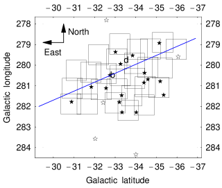
Figure 1: The 27 MACHO fields that we selected. The filled stars denote the positions of the microlensing events reported by the MACHO collaboration, while the empty stars are that of the EROS collaboration. The centers of the LMC bar and disk are labeled by “b” and “d”, respectively. The blue line marks the LMC bar major axis.

These fields (1, 2, 3, 5, 6, 7, 9, 10, 11, 12, 13, 14, 15, 17, 18, 19, 22, 23, 24, 47, 76, 77, 78, 79, 80, 81, 82 according to the MACHO numbering) have been selected taking into account the position of the microlensing events found towards the LMC by the MACHO collaboration during a $5.7$ years monitoring campaign (Alcock et al. 2000a).

Following the strategy of Gyuk et al. (2000), the values of the optical depths, found for each source/lens geometry, have been averaged on the 27 MACHO fields that we selected. The value for each field was obtained by computing the optical depth per unit surface and then by integrating over the area of the field.

• Model 1. The total optical depth, obtained using the “preferred” values for $M_{\mathrm{disk}}+M_{\mathrm{bar}}=3\times 10^{9}\,\mathrm{M}_{\sun}$ and an inclination angle of $30^{\circ}$, is $\tau=2.63\times 10^{-8}$ for the model $1a$ and $\tau=2.58\times 10^{-8}$ for the model $1b$. The results, summarized in Table 1, are in good agreement with the corresponding values found by Gyuk et al. (2000) as expected, since we adopted the same values for the LMC parameterization. There is a slight dependence on the LMC disk inclination, as it appears also from Fig. 2, which shows the variation of the total optical depth with the disk inclination.

  

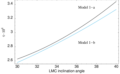
  Figure 2: Total optical depth for LMC self-lensing as a function of the LMC inclination angle for two different models assuming a total mass of $3\times 10^{9}\,\mathrm{M}_{\sun}$.

  If we use the upper limit for the LMC disk and bar masses, the corresponding total optical depth is clearly larger: $\tau=5.25\times 10^{-8}$ for the model $1a$ and $\tau=5.15\times 10^{-8}$ for the model $1b$. By appropriately choosing the parameters in the ranges specified in Sect. 2 Gyuk et al. (2000) found an upper value of about $\tau=8\times 10^{-8}$ for the self-lensing optical depth. Clearly, this implies to adopt rather unrealistic values for the parameters. We refer to Gyuk et al. (2000) for a detailed discussion on the self-lensing optical depth range as well as a comparison with the theoretical results appeared meanwhile in the literature.

  Table 1: Model 1: theoretical estimates of the optical depth, $\tau$, towards the LMC, averaged over 27 MACHO fields, for different source/lens geometries and parameters in the case of self-lensing.

  $Source/Lens$	$LMC\,mass$	$Model$	$LMC$	$Relative$	$\tau$
  $Geometry$	$(\times 10^{9}M_{\sun})$		$inclination$	$Weight$	$(\times 10^{-8})$
  $Disk/disk$	$3-6$	1a 1a 1a 1b 1b 1b	$30^{\circ}$ $35^{\circ}$ $40^{\circ}$ $30^{\circ}$ $35^{\circ}$ $40^{\circ}$	0.40 0.35 0.31 0.69 0.64 0.60	1.27 - 2.54 1.38 - 2.76 1.52 - 3.04 1.27 - 2.54 1.38 - 2.76 1.52 - 3.04
  $Disk/bar$	$3-6$	1a 1a 1a 1b 1b 1b	$30^{\circ}$ $35^{\circ}$ $40^{\circ}$ $30^{\circ}$ $35^{\circ}$ $40^{\circ}$	0.40 0.35 0.31 0.69 0.64 0.60	0.83 - 1.66 0.74 - 1.47 0.66 - 1.32 0.80 - 1.59 0.78 - 1.56 0.71 - 1.42
  $Bar/disk$	$3-6$	1a 1a 1a 1b 1b 1b	$30^{\circ}$ $35^{\circ}$ $40^{\circ}$ $30^{\circ}$ $35^{\circ}$ $40^{\circ}$	0.60 0.65 0.69 0.31 0.36 0.40	1.20 - 2.40 1.50 - 2.94 1.79 - 3.59 2.31 - 4.62 2.76 - 5.53 3.29 - 6.57
  $Bar/bar$	$3-6$	1a 1a 1a 1b 1b 1b	$30^{\circ}$ $35^{\circ}$ $40^{\circ}$ $30^{\circ}$ $35^{\circ}$ $40^{\circ}$	0.60 0.65 0.69 0.31 0.36 0.40	1.78 - 3.58 1.91 - 3.84 2.21 - 4.43 1.38 - 2.76 1.50 - 3.00 1.65 - 3.30
  $Total$	$3-6$	1a 1a 1a 1b 1b 1b	$30^{\circ}$ $35^{\circ}$ $40^{\circ}$ $30^{\circ}$ $35^{\circ}$ $40^{\circ}$	1 1 1 1 1 1	2.63 - 5.25 2.99 - 5.88 3.44 - 6.88 2.58 - 5.15 2.92 - 5.84 3.33 - 6.66

• Model 2. The total optical depth is $\tau=3.46\times 10^{-8}$ for the model $2a$ and $\tau=4.05\times 10^{-8}$ for the model $2b$ for the lower mass value. These values are quite similar to the ones found for model 1. The adopted parameters are described in Sect. 2 and the results are summarized in Table 2 for different source/lens geometries. As in the previous case, if we use the upper limit for the LMC disk and bar masses, the corresponding total optical depth gets larger and probably unrealistic for both models. Nonetheless, even in that case the observed value for the optical depth cannot be explained only by self-lensing.

Table 2: Model 2: theoretical estimates of the optical depth, $\tau$, towards the LMC, averaged over 27 MACHO fields, for different source/lens geometries and parameters in the case of self-lensing.

$Source/Lens$	$Model$	$LMC\,mass$	$Relative$	$\tau$
$Geometry$		$(\times 10^{9}\mathrm{M_{\sun}})$	$Weight$	$(\times 10^{-8})$
$Disk/disk$	2a 2b	3 - 6 3 - 5	0.50 0.20	2.14 - 4.61 1.34 - 2.40
$Disk/bar$	2a 2b	3 - 6 3 - 5	0.50 0.20	1.79 - 3.59 4.48 - 7.47
$Bar/disk$	2a 2b	3 - 6 3 - 5	0.50 0.80	1.31 - 2.63 0.82 - 1.36
$Bar/bar$	2a 2b	3 - 6 3 - 5	0.50 0.80	1.68 - 3.36 2.79 - 6.99
$Total$	2a 2b	3 - 6 3 - 5	1 1	3.46 - 7.10 4.05 - 8.65

The five events found so far by the EROS collaboration are all located quite far from the LMC central regions, see Fig. 1. Therefore, we expect the optical depth for self-lensing to be accordingly small. Indeed, using the model $1a$, the averaged self-lensing optical depth over the event positions is $0.8\times 10^{-8}$ for a LMC disk mass equal to $2.4\times 10^{9}\,\mathrm{M_{\sun}}$ or $1.6\times 10^{-8}$ for a LMC disk mass equal to $4.8\times 10^{9}\,\mathrm{M_{\sun}}$ (given the position of the EROS events the bar does not contribute). Clearly, these values are smaller than the corresponding ones for the MACHO fields and thus the EROS events are less likely to be due to self-lensing.

In Table 8 we give also the value for the optical depth due to MACHOs located in the LMC halo assuming a core radius $a$ equal to 2 kpc (it was found that the optical depth is quite insensitive to the variation of the core radius (Gyuk et al. 2000)) and that MACHOs make up 100% of the dark LMC halo, which is clearly an extreme assumption and has thus to be considered as an upper limit given also the fact that it is still not clear if the LMC has a halo at all. Moreover, this value is valid for a line of sight going through the center of the LMC and, therefore, also for that reason it has to be considered as an upper limit.

4.2 Number of events

By observing roughly 12 millions stars from 1992 to 1998, the MACHO collaboration found 13-17 microlensing events, according to the data-analysis criteria used ($A$ or $B$) (Alcock et al. 2000a). Instead, the EROS2 collaboration found 4 events monitoring about 25.5 millions of stars from 1996 to 1999 (Milsztajn & Lasserre 2001). Another event was found by EROS1 in the period 1990-1993 monitoring roughly 8 milion of stars (Aubourg et al. 1993). These results are summarized in the bar chart of Fig. 3, from which one sees that the detection of events with short duration ($\hat{t}<60\,\mathrm{days}$) is favoured.

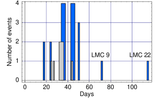
Figure 3: Bar chart of the number of observed microlensing events towards the LMC as a function of their duration. The full bars represent the seventeen MACHO events, while the gray bars represent the five EROS events.

Yet, the two MACHO events, LMC-9 and LMC-22, both with $\hat{t}>60\,\mathrm{days}$, must be treated with caution, because they are a binary event (Alcock et al. 2000b) and a possible exotic event (Alcock et al. 2000a), respectively.

We computed the number of self-lensing events, $N_{\mathrm{ev}}$, again by averaging over the 27 MACHO field as done for the optical depth. We used also the MACHO parameters: $N_{*}=11.9\times 10^{6}\,\mathrm{stars}$, $t_{obs}=5.7\,\mathrm{years}$, $\varepsilon=0.4-0.5$. We recall that the number of events is $N_{\mathrm{ev}}=N_{*}t_{\mathrm{obs}}\Gamma$, where $\Gamma$ is given by Eq. (30). For the mass distribution we used four different Salpeter-type IMFs as given in Eq. (22), with, as an illustration, different values for $\alpha$ and $\mu_{min}$:

• IMF-1 with $\mu_{\mathrm{min}}=0.1$ and $\alpha=0.56$ for $0.1<\mu<0.59$ and $\alpha=2.2$ for $\mu>0.59$;

• IMF-2 with $\mu_{\mathrm{min}}=0.1$ and $\alpha=2.35$;

• IMF-3 with $\mu_{\mathrm{min}}=0.01$ and $\alpha=0.8$ for $0.01<\mu<0.2$ and $\alpha=2.35$ for $\mu>0.2$;

• IMF-4 with $\mu_{\mathrm{min}}=0.01$ and $\alpha=2.35$.

• Model 1. The results for the different source/lens geometries, IMFs and parameters are shown in Table 3 for $\varepsilon=0.5$, $\sigma=30\,\mathrm{km/sec}$. For other values of $\varepsilon$ and $\sigma$ it is sufficient to rescale the numbers in the table by the new values of the parameters, since the number of events is proportional to $\varepsilon$ and $\sigma$.

  Table 3: Model 1: theoretical estimates of the LMC self-lensing number of events, $N_{\mathrm{ev}}$, averaged over 27 MACHO fields. We used $\varepsilon=0.5$ for the detection efficiency and $\sigma=30\,\mathrm{km\,sec^{-1}}$ for the velocity dispersion. Different source/lens geometries and four Salpeter-type IMFs with different slopes and minimal lens mass as described in the text were used.

  $Source/Lens$	$LMC\,mass$	$Model$	$LMC$	$Relative$	$N_{\mathrm{ev}}$	$N_{\mathrm{ev}}$	$N_{\mathrm{ev}}$	$N_{\mathrm{ev}}$
  $Geometry$	$(\times 10^{9}\mathrm{M_{\sun}})$		$inclination$	$Weight$	$(\mathrm{IMF-1})$	$(\mathrm{IMF-2})$	$(\mathrm{IMF-3})$	$(\mathrm{IMF-4)}$
  $Disk/disk$	$3-6$	1a 1a 1b 1b	$30^{\circ}$ $35^{\circ}$ $30^{\circ}$ $35^{\circ}$	0.40 0.35 0.69 0.64	0.60-1.20 0.60-1.35 0.60-1.20 0.60-1.35	1.50-2.85 1.50-3.00 1.50-2.86 1.50-3.00	1.62-3.23 1.72-3.44 1.62-3.23 1.72-3.44	4.35-8.85 4.65-9.45 4.35-8.85 4.65-9.45
  $Disk/bar$	$3-6$	1a 1a 1b 1b	$30^{\circ}$ $35^{\circ}$ $30^{\circ}$ $35^{\circ}$	0.40 0.35 0.69 0.64	0.45-1.05 0.45-0.75 0.15-0.30 0.15-0.15	1.20-2.25 0.90-1.80 0.30-0.60 0.30-0.45	1.31-2.63 1.04-2.08 0.33-0.66 0.30-0.60	3.60-7.20 2.85-5.70 0.90-1.80 0.75-1.65
  $Bar/disk$	$3-6$	1a 1a 1b 1b	$30^{\circ}$ $35^{\circ}$ $30^{\circ}$ $35^{\circ}$	0.60 0.65 0.31 0.36	0.90-1.80 1.35-2.55 2.25-4.50 2.85-5.70	2.10-4.35 3.00-6.00 5.10-10.2 6.60-13.1	2.50-5.00 3.47-6.94 5.95-11.9 7.57-15.1	6.75-13.7 9.45-19.1 16.4-32.6 20.7-41.4
  $Bar/bar$	$3-6$	1a 1a 1b 1b	$30^{\circ}$ $35^{\circ}$ $30^{\circ}$ $35^{\circ}$	0.60 0.65 0.31 0.36	1.05-2.10 1.20-2.25 0.75-1.35 0.75-1.50	2.40-4.80 2.55-5.35 1.50-3.15 1.65-3.45	2.81-5.62 3.03-6.06 1.81-3.62 1.97-3.93	7.65-15.5 8.25-16.7 4.95-9.90 5.40-10.8
  $Total$	$3-6$	1a 1a 1b 1b	$30^{\circ}$ $35^{\circ}$ $30^{\circ}$ $35^{\circ}$	1 1 1 1	1.65-3.30 2.10-3.90 1.50-2.85 1.80-3.60	3.75-7.50 4.35-9.00 3.30-6.45 4.05-8.10	4.36-8.72 5.19-10.4 3.75-7.50 4.72-9.44	11.9-23.9 14.1-28.5 10.2-20.6 12.9-25.9

  The IMF-1 is not very realistic since it is based upon counts of M class stars in the Galactic disk (Gould et al. 1997) and should thus be taken just as an illustration. Moreover, as can be inferred from Table 3, for the IMF-1 mass distribution the number of events is less than for the the more realistic IMF-2 and IMF-3 cases. The IMF-4 is also not very realistic, leading already for a rather small dispersion velocity to a conspicuous number of events. However, as we will see below, the resulting average event duration for the IMF-4 is definitely not in agreement with the observed value.

  For the IMF-2 and the IMF-3 we see that even by considering the more extreme values for the various parameters we get at most about 10 events, which is still less then the ones reported by the MACHO group although not very much. However, this implies to adopt rather unlikely values for the various LMC parameters. For the preferred and more realistic values, leading to an optical depth of $\tau\simeq 2-3\times 10^{-8}$, we expect about 3 to 5 events due to self-lensing (Table 3).

• Model 2. For the model 2, on the ground of the results from the previous section, we concentrate only on the more realistic models for self-lensing by using IMF-2 and IMF-3. The results for the different source/lens geometries are shown in Table 4 for model $2a$ and $2b$, where we fixed again the detection efficiency to 0.5 and the velocity dispersion to 30 km/sec. We see that also these models lead to values which are similar to the ones of model 1 and thus are also not able to explain all the observed MACHO events. For the model 2 we expect again rougly $3$ events due to self-lensing when using the lower value for the LMC mass. Thus it seems that this conclusion is rather robust and does not depend much on the detailed form of the bar and the disk.

Table 4: Model 2: estimates of the total number of microlensing events towards LMC for the MACHO observation time computed in the case of self-lensing and for different values of the velocity dispersion, LMC mass and efficiency. We used $\varepsilon=0.5$ for the detection efficiency and $\sigma=30\,\mathrm{km\,sec^{-1}}$ for the velocity dispersion. Two Salpeter-type IMFs were used (see text for the values of the parameters).

$Source/Lens$	$LMC\,mass$	$Model$	$Relative$	$N_{\mathrm{ev}}$	$N_{\mathrm{ev}}$
$Geometry$	$(\times 10^{9}\mathrm{M_{\sun}})$		$Weight$	$(\mathrm{IMF-2})$	$(\mathrm{IMF-3})$
$Disk/disk$	3 - 6 3 - 5	2a 2b	0.50 0.20	2.38 - 4.77 1.49 - 2.48	2.76 - 5.53 1.73 - 2.88
$Disk/bar$	3 - 6 3 - 5	2a 2b	0.50 0.29	0.58 - 1.17 1.46 - 2.43	0.68 - 1.35 1.69 - 2.82
$Bar/disk$	3 - 6 3 - 5	2a 2b	0.50 0.80	2.11 - 4.23 1.32 - 2.21	2.45 - 4.91 1.53 - 2.56
$Bar/bar$	3 - 6 3 - 5	2a 2b	0.50 0.80	0.61 - 1.22 1.52 - 2.53	0.70 - 1.41 1.76 - 2.93
$Total$	3 - 6 3 - 5	2a 2b	1 1	2.84 - 5.70 2.86 - 4.77	3.30 - 6.60 3.32 - 5.53

Similarly, we can estimate the number of self-lensing events we expect for the EROS2 data for a disk/disk source lens geometry. In this case, using the IMF-2 and an efficiency equal to about 0.12 (see Milsztajn & Lasserre 2001), the estimated number of events, using the model $1a$, is $0.16-0.32$ for $\sigma=30\,\mathrm{km/sec}$ and for a LMC disk mass in between $2.4-4.8\times 10^{9}\mathrm{M_{\sun}}$. For the IMF-3 the corresponding number of events is $0.19-0.37$. If instead we use the model $2a$, we expect for the above parameters a number of events equal to $0.23-0.46$ using the IMF-2, and $0.27-0.53$ using the IMF-3. Finally, we expect $0.14-0.24$ and $0.17-0.28$ for the model 2b and for IMF-2 and IMF-3, respectively. Even if the small number of events found by EROS2 does not allow to draw a definitive conclusion, it seems unlikely that the EROS2 events are all due to self-lensing.

We computed also the expected number of events due to MACHOs in the LMC halo. The lens number density is given by

$$\frac{dn}{d\mu}=\left(1+\frac{R^{2}}{a^{2}}\right)^{-1}\frac{dn_{0}}{d\mu},$$ (45)

where for $dn_{0}/d\mu$ we assume a delta function, and fix $a$ equal to 2 kpc (Gyuk et al. 2000) (see Table 9). Using the MACHO collaboration parameters and $\mu=0.5$ we expect roughly 5 events under the assumption of a 100% MACHO LMC halo and assuming that the rate is uniformly equal to the one for the line of sight going through the center of the LMC, this last assumption obviously leads to an upper limit. Clearly, since the halo mass fraction in form of MACHOs in the halo of our Galaxy is at most 20% (Alcock et al. 2000a), we do not expect this fraction to be higher in the LMC halo. Thus, realistically we expect at most about 1 event coming from this component. A similar conclusion holds for the EROS2 data.

4.3 Average event duration

Using the Eq. (41) we get estimates of the average event duration $<T>$ for different source/lens geometries and IMFs. The results, averaged on 27 MACHO field, are shown in Table 5 for model 1 and in Table 7 for model 2. The velocity dispersion is in both cases assumed to be $30\,\mathrm{km/sec}$.

Table 5: Model 1: theoretical estimates of the LMC self-lensing event durations, $<T>$, averaged over 27 MACHO fields. We used $\sigma=30\,\mathrm{km\,sec^{-1}}$ for the velocity dispersion. Different source/lens geometries and four Salpeter-type IMFs were used (For the parameters see text). The durations are given in days.

$Source/Lens$	$Model$	$LMC$	$<T>$	$<T>$	$<T>$	$<T>$
$Geometry$		$inclination$	$(IMF-1)$	$(IMF-2)$	$(IMF-3)$	$(IMF-4)$
$Disk/disk$	1a 1a 1b 1b	$30^{\circ}$ $35^{\circ}$ $30^{\circ}$ $35^{\circ}$	67.3 68.8 67.3 68.8	49.5 50.7 49.5 50.7	42.9 43.9 42.9 43.9	19.9 20.3 19.9 20.3
$Disk/bar$	1a 1a 1b 1b	$30^{\circ}$ $35^{\circ}$ $30^{\circ}$ $35^{\circ}$	59.6 60.7 63.4 64.3	43.9 44.7 46.7 47.3	38.0 38.7 40.4 41.0	17.6 17.9 18.7 19.0
$Bar/disk$	1a 1a 1b 1b	$30^{\circ}$ $35^{\circ}$ $30^{\circ}$ $35^{\circ}$	75.1 80.4 82.3 87.1	55.3 59.2 60.6 64.1	47.9 51.3 52.5 55.5	22.2 23.7 24.3 25.7
$Bar/bar$	1a 1a 1b 1b	$30^{\circ}$ $35^{\circ}$ $30^{\circ}$ $35^{\circ}$	54.3 54.3 65.4 65.3	40.0 40.0 48.1 48.1	34.6 34.6 41.7 41.7	16.0 16.0 19.3 19.3
$Average$	1a 1a 1b 1b	$30^{\circ}$ $35^{\circ}$ $30^{\circ}$ $35^{\circ}$	64.1 66.1 69.6 71.4	47.2 48.7 51.2 52.6	40.9 42.1 44.4 45.5	18.9 19.5 20.6 21.1

• Model 1. In Fig. 4 we report the average event duration obtained using the four considered IMFs and different values of the velocity dispersions.

  

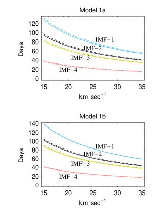
  Figure 4: Model 1: variation of the total self-lensing event durations as a function of the velocity dispersion. The solid lines and the dashed lines are obtained by using a LMC disk inclination of $30^{\circ}$ and $35^{\circ}$, respectively. Four different IMFs were used (for the parameters see text). Two models ($1a$ and $1b$) are shown separately.

  We recall that the IMF-1 was deduced by dwarf star counts in the Milky Way disk, so we must be cautious when applying it to a population of another galaxy like LMC.

  The results in Fig. 4 can not be directly compared with the observed MACHO event durations as summarized in Table 6, because among them there are two events, LMC-9 (binary event) and LMC-22 (exotic event), which are not compatible with our method of analysis and there is one more event, LMC-5 (disk event) which is not a self-lensing event.

  Table 6: EROS and MACHO (blended and unblended) average event durations. The quantity $\hat{t}_{st}(A,B)$ is the average event timescale, according to the two different criteria used in the efficiency, for events in the MACHO Monte Carlo calculations that have been detected with an unblended fit timescale of $\hat{t}$.

  $Team$	$Set$	$N_{\mathrm{ev}}$	$<T>$
  EROS	$\hat{t}$	$5$	$33\,\mathrm{days}$
  MACHO	$\hat{t}$	$17$	$44\,\mathrm{days}$
  MACHO	$\hat{t}_{st}(A)$	$13$	$47\,\mathrm{days}$
  MACHO	$\hat{t}_{st}(B)$	$17$	$56\,\mathrm{days}$

  So, we must exclude these three events from the MACHO blended average event durations, set $\hat{t}$, before comparing with our results. The remaining $14$ events give an average duration of $37\,\mathrm{days}$. Moreover, as mentioned above (see also Fig. 3) all relevant events have a duration in between 18 and 52 days. Comparing this with our results (Fig. 4) and taking also into account that not all events are possibly due to self-lensing, clearly leads already to restrictions on the IMF and in particular on the velocity dispersion values: the velocity dispersion is more likely to be in the range of $30-35\,\mathrm{km/sec}$, that suggests a predominance of lenses of old population (Hughes et al. 1991) and IMF-2 or IMF-3 are favored, since IMF-1 leads to too high durations. On the other hand an IMF-4 model would require a low velocity dispersion (below $20\,\mathrm{km/sec}$), otherwise the average duration gets substantially below the observed value. However, for very low mass objects one would rather expect a higher velocity dispersion.

• Model 2.

  For this model we consider three IMFs: IMF-2, IMF-3 and IMF-4. The results, reported in Table 7 and in Fig. 5, show that the mean durations are slightly lower than that of model 1, nonetheless the previous conclusions hold.

Table 7: Model 2: theoretical estimates of the LMC self-lensing durations of events, $<T>$, averaged over 27 MACHO fields. We used $\sigma=30\,\mathrm{km\,sec^{-1}}$ for the velocity dispersion. Various source/lens geometries and three Salpeter-type IMFs were used (for the parameters see text). The durations are given in days. (We do not distinguish between model 2a and 2b, since both give the same results.)

$Source/Lens$	$<T>$	$<T>$	$<T>$
$Geometry$	$(IMF-2)$	$(IMF-3)$	$(IMF-4)$
$Disk/disk$	$52.6$	$45.6$	$21.1$
$Disk/bar$	$46.3$	$40.1$	$18.5$
$Bar/disk$	$33.8$	$29.3$	$13.6$
$Bar/bar$	$41.6$	$36.0$	$16.7$
$Average$	$43.6$	$37.8$	$17.5$

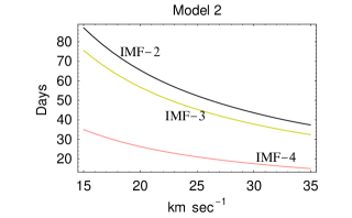
Figure 5: Model 2: variation of the total self-lensing event duration as a function of the velocity dispersion. These curves are obtained by using a LMC disk inclination of $35^{\circ}$. Three different IMFs were used (for the parameters see text).

We arrive at the same conclusion also if we compare our results with the EROS mean event duration (see Table 6) under the rather unplausible hypothesis that they are all due to self-lensing.

For the IMF-4 mass distribution we see from Fig. 4 that the duration of events decreases slowly by increasing the velocity dispersion of the lenses and in order to explain the observed mean duration of the events requires a low ($\sigma<20\,\mathrm{km/sec}$) velocity dispersion. For what we saw in the previous section on the IMF-4 model this would then also imply that all the detected events are due to self-lensing. However, such a low required dispersion velocity is rather unplausible considering also the small mass of the lenses. Thus the IMF-4 model is certainly not very realistic.

Using the number density given by Eq. (45), we estimated the event duration also for lenses in the LMC halo, see Table 9. We expect a duration in between $128\sqrt{\mu}$ and $181\sqrt{\mu}$ days according if we take into account the motion of the source as in the former case or not.

4.4 Self-lensing mean mass

With the mass moment method we are able to get an estimate of the lens mean mass $<M>$, as given by Eq. (42). We notice that to get this way the mean mass we do clearly not need to assume a particular IMF distribution. For $<T^{1}>$ and $<T^{-1}>$, we used the Einstein radius crossing times measured by the MACHO collaboration for the 17 events that they detected (Alcock et al. 2000a). Some of them were excluded in our LMC self-lensing analysis: the Galactic disk event LMC-5, the binary event LMC-9, and the exotic event LMC-22 (probably the source is a distant active galaxy (Bennett 2001)). With this exclusion, the events LMC-1 and LMC-15 have the shortest duration, while the events LMC-7, LMC-13 and LMC-14 have the longest duration. Moreover, LMC-14 is a self-lensing event (Alcock et al. 2001b). In Section 4.2 we saw that the expected number of self-lensing events is at least 3. Assuming thus that among the observed events (not including the 3 excluded ones as explained above, one of which being also probably a self-lensing) just 3 are due to self-lensing, we can estimate a minimum and a maximum mean mass using the following 3 events: LMC-1, LMC-14, LMC-15 (mean duration: 28.5 days) for $<M_{\mathrm{min}}>$, and LMC-7, LMC-13, LMC-14 (mean duration: 50.5 days) for $<M_{\mathrm{max}}>$.

In Fig. 6 we report the results for different values of the velocity dispersion obtained using models $1a$, $1b$ and $2$ (we do not distinguish between model $2a$ and $2b$, since both give the same results).

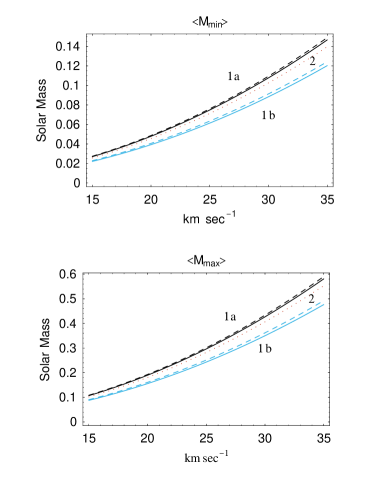
Figure 6: Total mean minimal and maximal mass of the lenses in solar mass unity as a function of the velocity dispersion (km/sec) for models $1a$, $1b$ and $2$ (dotted line). For the models $1a$ and $1b$, the solid lines and the dashed lines are obtained by using a LMC disk inclination of $30^{\circ}$ and $35^{\circ}$, respectively.

Any other combination in the choice of the events (or in particular by assuming that more than 3 events are due to self-lensing) would lead to a higher value for $<M_{\mathrm{min}}>$ and to a lower value for $<M_{\mathrm{max}}>$. Thus the values given here have to be considered as lower and upper limit, respectively. These results have a slight dependence from the LMC disk inclination, as it appears from Fig. 6, which shows also the variation of the mean mass for a disk inclination between $30^{\circ}-35^{\circ}$.

We see that for our preferred values for the LMC mass and for $\sigma\simeq 30-35\,\mathrm{km\,sec^{-1}}$, we get a mass in the range $\sim 0.1-0.6\,\mathrm{M_{\sun}}$, which is consistent with the various assumptions we made. This result suggests that the lenses are low mass stars, which is certainly not surprising This can also be seen as a consistency check on the modelling of the LMC we adopted.

5 Galactic and halo lensing populations

In this section we turn to the case that some of the lenses are located in the Milky Way or in its halo. A Galactic model with three main components fits well all the dynamical observations. These components are the disk, the spheroid and the halo. The halo, composed essentially of dark matter, contributes for most part of the total mass of the Galaxy and should give the higher contribution to the microlensing surveys. However, since at least one event (LMC-5) is due to a Galactic disk lens (Alcock et al. 2001c), we will examine two other important Galactic components: disk (thin and thick) and spheroid. In Tables 8 and 9 we summarize the estimates of the microlensing quantities related to these components. The thin and thick disks are considered as separate components.

There is no general agreement on the details of the structure of our Galaxy and in particular on the parameters of its thick disk and spheroid. For the disk we vary the structural parameters in a wide range, while for the spheroid we refer to Giudice et al. (1994), where the modelling of this component is amply discussed. Moreover, we refer to Carrol & Ostlie (1996), Roulet & Mollerach (1997) and Sparke & Gallagher (2000) for most of the parameters used to describe the Galactic components.

Table 8: Theoretical estimates of the optical depth for stars in the LMC due to different lensing populations: thin disk, thick disk, spheroid (stellar halo), MW halo and LMC halo.

$Lensing\,component$	$\Sigma_{0}\,(\mathrm{M_{\sun}pc^{-2}})$	$\rho_{0}\,(\mathrm{M_{\sun}pc^{-3}})$	$\tau$
$Thin\,Disk$	$(30-50)$	$-$	$(0.92-1.54)\times 10^{-8}$
$Thick\,Disk$	$(35-45)$	$-$	$(3.09-3.97)\times 10^{-8}$
$Spheroid$	$-$	$0.0015\times 10^{-3}$	$4.29\times 10^{-8}$
$MW\,halo$	$-$	$0.0079\times 10^{-3}$	$4.83\times 10^{-7}$
$LMC\,halo$	$-$	$0.0223\times 10^{-3}$	$8.36\times 10^{-8}$

Table 9: Theoretical estimates of the number of events and event mean duration for LMC stars by different lensing populations: thin disk, thick disk, spheroid (stellar halo), MW halo and LMC halo. A $\delta$-function was used to describe the mass distribution of the lenses in the halos. Instead, two IMFs with different slopes were used to describe the other Galactic components. Different values for the dispersion velocity, $\sigma$, were used. $\varepsilon$ is the MACHO detection efficiency and $\mu$ is the lens mass in solar mass units.

$Component$	$\sigma$	$dn_{0}/d\mu$	$\mbox{MACHO}\,N_{\mathrm{ev}}$	$\mbox{EROS}\,N_{\mathrm{ev}}$	$<T>$
$Thin\,Disk$	$(20-30)\,\mathrm{km\,sec^{-1}}$	IMF-1 IMF-2	$(0.3-0.4)$ $\varepsilon$ $(0.9-1.4)$ $\varepsilon$	$0.04-0.05$ $0.12-0.18$	$(107-71)$  $\mathrm{days}$ $(78-52)$   $\mathrm{days}$
$Thick\,Disk$	$(35-60)\mathrm{km\,sec^{-1}}$	IMF-1 IMF-2	$(1.5-2.5)$ $\varepsilon$ $(3.3-5.7)$ $\varepsilon$	$0.2-0.3$ $0.5-0.8$	$(103-60)$  $\mathrm{days}$ $(76-44)$  $\mathrm{days}$
$Spheroid$	$(90-120)\,\mathrm{km\,sec^{-1}}$	IMF-1 IMF-2	$(2.8-3.8)$ $\varepsilon$ $(6.5-8.7)$ $\varepsilon$	$0.4-0.5$ $0.9-1.2$	$(69-52)$  $\mathrm{days}$ $(51-38)$  $\mathrm{days}$
$MW\,halo$	$210\,\mathrm{km\,sec^{-1}}$	$\delta$	$107.7\,\varepsilon\,\mu^{-1/2}$	$14.6\,\mu^{-1/2}$	$71\,\sqrt{\mu}\,\mathrm{days}$
$LMC\,halo$	$\mathrm{50\,km\,sec^{-1}}$	$\delta$	$7.3\,\varepsilon\mu^{-1/2}$	$1.0\,\mu^{-1/2}$	$(128-181)\,\sqrt{\mu}\,\mathrm{days}$

5.1 Lenses in the Galactic Thick Disk

We start our analysis on galactic components with the hypothesis that some lenses are associated with the oldest sub-population of the Galactic disk. We consider that these lenses, a fraction of which might be high velocity white dwarfs (Reid et al. 2001), are confined within the so-called thick disk. In this case, we used a lens number density distribution per unit mass $dn/d\mu$ given by

$$\frac{dn}{d\mu}=H_{\mathrm{TD}}\frac{dn_{0}}{d\mu}=$$

$$= \exp\left[-\frac{\sqrt{R_{0}^{2}+D_{\mathrm{ol}}^{2}\cos^{2}{b}-2R_{0}D_{\mathrm{ol}}\cos{b}\cos{l}}}{R_{\mathrm{TD}}}\right]\times$$

$$\times \exp\left[\frac{R_{0}}{R_{\mathrm{TD}}}\right]\exp\left[-\frac{|D_{\mathrm{ol}}\sin{b}|}{z_{\mathrm{TD}}}\right]\frac{dn_{0}}{d\mu},$$

where $R_{0}$ is the Earth distance from the center of the Galaxy, for which we use the IAU recommended value of $8.5$ kpc. The common value for the thick disk scale length $R_{\mathrm{TD}}$ is $3.5\,\mathrm{kpc}$ (Bahcall 1986), even if its estimate varies in a wide range. Here, we will vary $R_{\mathrm{TD}}$ in between 2 and 5 kpc. The thick disk has a larger scale height as compared to the thin disk. Its value is generally estimated to be in the range $1<z_{\mathrm{TD}}<1.5$ kpc. For the local column density we use $\Sigma_{0}^{\mathrm{TD}}=35-45\,\,\mathrm{M_{\sun}\,pc^{-2}}$ (Derue et al. 2001; Roulet & Mollerach 1997). All the estimates of microlensing quantities for $R_{\mathrm{TD}}=3.5$ kpc, and $z_{\mathrm{TD}}=1$ (Bahcall 1986), are reported in Tables 8 and 9.

In Fig. 7 we plotted the variation of the optical depth as a function of $R_{\mathrm{TD}}$ for different values of $\Sigma_{0}^{\mathrm{TD}}$ and with values for $z_{\mathrm{TD}}$ equal to 1 kpc (Fig. 7a) and to 1.5 kpc (Fig. 7b), respectively.

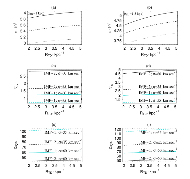
Figure 7: Galactic thick disk microlensing quantities as a function of the scale length, $R_{\mathrm{TD}}$, for different local column densities, IMFs, dispersion velocities, and for the scale height, $z_{\mathrm{TD}}$, equal to 1 kpc (a, c, e) and 1.5 kpc (b, d, f). MACHO collaboration experimental values were used. Here we take the detection efficiency $\varepsilon$ equal to 0.5. (a, b) Optical depth: the solid line was estimated for $\Sigma_{0}^{\mathrm{TD}}=45\,\mathrm{M}_{\sun}\,\mathrm{pc}^{-2}$, the dashed line for $\Sigma_{0}^{\mathrm{TD}}=40\,\mathrm{M}_{\sun}\,\mathrm{pc}^{-2}$, and the dotted line for $\Sigma_{0}^{\mathrm{TD}}=35\,\mathrm{M}_{\sun}\,\mathrm{pc}^{-2}$. (c, d) Number of events. (e, f) Mean duration of events.

From these figures one sees that the optical depth varies little with the scale length $R_{\mathrm{TD}}$. Instead, there is a more clear dependence of $\tau$ on the value of the scale height $z_{\mathrm{TD}}$, besides also the density. This is true also for the number and the mean duration of events, Fig. 7c-d and Fig. 7e-f respectively, even if in these cases the parameters on which one has to vary are connected to the IMF and the dispersion velocity of the lenses.

For $R_{\mathrm{TD}}=3.5$ kpc, $z_{\mathrm{TD}}=1$, and $\Sigma_{0}^{\mathrm{TD}}=35-45\,\mathrm{M_{\sun}\,pc^{-2}}$, we found that the optical depth towards the LMC is $\tau=3.09-3.97\times 10^{-8}$ (Table 8), that is higher than the estimated white dwarf population optical depth $\tau\approx 0.4\times 10^{-8}$ (Koopmans & Blandford 2001).

Following the discussion in Sect. $3.3$, for the mass distribution we used two Salpeter type IMFs: IMF-1 with $\alpha=0.56$ for $0.1<\mu<0.59$ and $\alpha=2.2$ for $\mu>0.59$; IMF-2 with $\alpha=2.35$. For MACHO experimental numbers, in Fig. 7 we report the variation of the number of events as a function of $R_{\mathrm{TD}}$ for different values of $\sigma$ and adopting $\varepsilon=0.5$ (Alcock et al. 2000a), $z_{\mathrm{TD}}$ equal to 1 kpc (Fig. 7c) and to 1.5 kpc (Fig. 7d).

Here and in the next section, clearly the use of IMF-1 is favoured, because it was obtained from Galactic disk observations, as we already mentioned in Sect. 4.2. In this case, joining thin and thick disk, we expect $1-3$ events for $R_{\mathrm{TD}}=3.5$ kpc, $z_{\mathrm{TD}}=1$, and for the velocity dispersion in the range $\sigma_{\mathrm{TD}}=35-60\,\mathrm{km\,sec^{-1}}$ (Derue et al. 2001; Carrol & Ostlie 1996).

At last, we estimated the mean duration of the events as a function of $R_{\mathrm{TD}}$ for different values of $\sigma$ and adopting $z_{\mathrm{TD}}$ equal to 1 kpc (Fig. 7e) and to 1.5 kpc (Fig. 7f). It seems that a disk event was really observed, LMC-5 (Alcock et al. 2001c). Its duration, $37.8\,\mathrm{days}$, is not in good agreement with our predictions (Table 9), however one can not draw any conclusion on just one event. Moreover, we assumed a minimum mass in the IMF-1 of 0.1 $\mathrm{M}_{\sun}$, whereas from the observation it turns out that the lens mass could well be below that limit, explaining thus its shorter duration.

5.2 Lenses in the Galactic Thin Disk

We consider now the possibility to have lenses in the thin disk. This component, contrary to the thick disk that is composed of low metallicity stars, is made of relatively young metal-rich stars with a small velocity dispersion $\sigma_{\mathrm{td}}\simeq 20-30\,\mathrm{km\,sec^{-1}}$ (Roulet & Mollerach 1997). We modelled it as in the previous case, see Eq. (5.1), but with a smaller scale height $z_{\mathrm{td}}=0.1-0.35\,\mathrm{kpc}$ (Roulet & Mollerach 1997) and with a local column density $\Sigma_{0}^{\mathrm{td}}=30-50\,\mathrm{M_{\sun}\,pc^{-2}}$ (Roulet & Mollerach 1997; Derue et al 2001).

For the thick disk we saw that the microlensing quantities do not vary much as a function of the scale length, but there were variations with the scale height. For the thin disk the scale length is know with only a small range of uncertainty and, therefore, the modifications on our theoretical estimates will be negligible. Here we use $z_{\mathrm{td}}=0.3\,\mathrm{kpc}$ (Bahcall 1986), and the optical depth turns out to be $\tau=0.9-1.5\times 10^{-8}$, see Table 8.

Using again two different IMFs as in the previous case, we estimated the number of events and their mean duration. The results are reported in Table 9. We see that the expected average event duration for both the thick and thin disk components is above 50 days when considering the more realistic IMF-1, so that it is rather unlikely that more than 1-2 events among the observed ones can be due to these populations, unless there are a lot of brown dwarfs, but these would have been discovered in the same way as in the case of the LMC-5 event.

5.3 Lenses in the Galactic Spheroid

Here we examine microlensing events by the stellar halo, i.e. the so-called Galactic spheroid. Looking at high latitudes far above the disk, there is a population of globular clusters, old metal-poor stars or high-velocity stars, supported by a large velocity dispersion, $\sigma_{\mathrm{sp}}\simeq(90-120)\,\mathrm{km\,sec^{-1}}$ (Carrol & Ostlie 1996; Roulet & Mollerach 1997). The spheroid, approximately spherical, provides an important contribution to the size of the central part of the Milky Way, while its radial extension is smaller than that of the halo. Dynamical measurements and infrared surveys predict for the spheroid a mass roughly equal to $5-7\times 10^{10}\mathrm{M}_{\sun}$, larger than that estimated on the basis of star counts. This suggests that the spheroid must be heavy and mostly dark (Caldwell & Ostriker 1981; Bahcall et al. 1983).

Giudice et al. (1994) have already discussed in some detail the possibility to have lenses in the spheroid. Using five different models based on the works of Caldwell & Ostriker (1981), Rohlfs and Kreitschmann (1988), Bahcall et al. (1983), they estimated the main microlensing quantities: an optical depth in the range $(3.1-4.9)\,\times 10^{-8}$, an event rate in the range $(0.01-0.16)/\sqrt{\mu}\,\frac{events}{yr\,10^{6}stars}$, an average event duration in the range $(66-71)/\sqrt{\mu}$ days, where $\mu$, as usual, is the lens mass in solar mass units.

Here we adopt the same simplified density profile, which fits well the Ostriker and Caldwell model as that in Roulet & Mollerach (1997), given by

$$\frac{dn}{d\mu} = H_{\mathrm{sp}}\frac{dn_{0}}{d\mu}=$$

$$= \left(\frac{\sqrt{R_{0}}+\sqrt{R_{\mathrm{c}}}}{\left(R_{0}^{2}+D_{\mathrm{ol}}^{2}-2R_{0}D_{\mathrm{ol}}\cos{\vartheta}\right)^{1/4}+\sqrt{R_{\mathrm{c}}}}\right)^{7},$$

where $R_{\mathrm{c}}\simeq 0.17\,\mathrm{kpc}$ is the core radius (Roulet & Mollerach 1997) and $\vartheta=82^{\circ}$ is the angle between the line of sight of the LMC and the direction of the Galactic center. In this case, using a local density equal to $\rho_{0}^{\mathrm{sp}}=1.5\times 10^{-3}\,\mathrm{M_{\sun}\,pc^{-3}}$, our estimate for the optical depth is $\tau=4.29\times 10^{-8}$, (see Table 8) which is in good agreement with the results of Giudice et al. (1994) and lies well within the range they found.

Also in this case we used two different IMFs to estimate the number of events and their mean duration. The results are reported in Table 9 from which we see that the average duration is somewhat higher than the observed value, unless the dispersion velocity is closer to $120\,\mathrm{km\,sec^{-1}}$ (or if the IMF goes well into the brown dwarf region). In this latter case some (2 to 6 events) among the MACHO longer duration events, close to about 40-50 days, could be due to lenses in the spheroid. This result is still in a good agreement with Giudice et al. (1994). Similarly, we expect at most 1 to 2 EROS events to belong to the spheroid. Clearly, given the calculated mean event duration and number of expected events we see that it is well plausible that some of the observed events are due to lenses located in the spheroid, however, certainly not all of them.

5.4 Lenses in the Galactic Halo

At last we estimated the microlensing quantities in the hypothesis that the lenses are MACHOs located in the Galactic halo (Jetzer 1996). The MACHO number density distribution that we used is now

$$\frac{dn}{d\mu} = H_{\mathrm{halo}}\frac{dn_{0}}{d\mu}=$$

$$= \frac{R_{\mathrm{c}}^{2}+R_{0}^{2}}{R_{\mathrm{c}}^{2}+R_{0}^{2}+D_{\mathrm{ol}}^{2}-2D_{o\mathrm{l}}R_{\mathrm{c}}\cos{\vartheta}}\frac{dn_{0}}{d\mu},$$

where $\vartheta=82^{\circ}$ is again the angle between the line of sight and the direction of the Galactic center and $R_{\mathrm{c}}$ is the core radius of the dark matter, that is also uncertain. Bahcall et al. (1983) estimated $R_{\mathrm{c}}$ equal to 2 kpc, while Caldwell & Ostriker (1981) suggested 7.8 kpc. Alcock et al. (2000a) used instead 5 kpc. Here, following Primack et al. (1988), we use a core radius equal to 5.6 kpc. For $dn_{0}/d\mu$, we used a delta function, Eq. (21), with $\rho_{0}^{\mathrm{H}}=7.9\times 10^{-3}\,\mathrm{M_{\sun}\,pc^{-3}}$.

Fixing the usual halo value for the velocity dispersion, $\sigma_{\mathrm{H}}=210\,\mathrm{km\,sec^{-1}}$, we estimated the optical depth, the number of events and the mean time duration. The results are tabulated in Tables 8 and 9. For $\mu=0.5\,\mathrm{M_{\sun}}$ (as an illustration) we expect for a halo made entirely of MACHOs 61 events using MACHO efficiency $\varepsilon=0.4$, and 76 events using MACHO efficiency $\varepsilon=0.5$, respectively. Similarly for EROS2, where we use an efficiency equal to $\varepsilon=0.12$, we expect 19 events. The expected mean event duration is $50\,\mathrm{days}$ for $\mu=0.5$.

For the optical depth we get the well-known value of $\approx 5\times 10^{-7}$, while the estimated optical depth for a halo white dwarf population is $\tau=0.13\times 10^{-8}$ (Koopmans & Blandford, 2001).

6 Mean Mass

From the previous discussion it is clear that almost certainly not all the observed events (in particular among the ones detected by the MACHO collaboration) originate from the same lens population. Accordingly, it is difficult to estimate a mean value for the mass, since we do not know in general to which population each event belongs. In the following we will consider different possibilities of how to divide the events among the various populations and so get estimates of the masses using the mass moment method. Clearly this has to be considered as an illustration, nonetheless it allows to get some insight and also to get some upper and lower limits which can already be useful.

The five EROS events, due to their positions (see Fig. 1) and durations, can hardly contain self-lensing and Galactic disk lenses. So most of them if not all (with perhaps the possibility of having 1 or 2 events due to the spheroid) are MACHOs in the Galactic halo, in which case we find the following mean mass: $<M>=0.26\,\mathrm{M_{\sun}}$, assuming a spherical halo model. If the 1 or 2 events with the longer duration are due to lenses in the galactic spheroid then of course we would get a smaller average mass for the remaining 3 to 4 halo events.

The MACHO events contain most probably some lenses in the LMC and at least one event due to a Galactic component. We exclude as before from our analysis the MACHO events LMC-9 and LMC-22, whereas LMC-14, is possibly a self-lensing event. We will consider, as an illustration, four different models by dividing up the observed events among the various populations, we shall label them with: M-1, M-2, M-3 and M-4 (see below).

We already saw in section 4.4 that we expect at least $3$ self-lensing events. For these three events, fixing the LMC dispersion velocity to $30\,\mathrm{km/sec}$ and clearly assuming that one of them is the LMC-14 event, we estimated a minimum (models M-1 and M-3 in which LMC-1, LMC-14 and LMC-15 are the self-lensing events) and a maximum (models M-2 and M-4 in which LMC-7, LMC-13 and LMC-14 are the self-lensing events) mean mass, see Table 10 and Fig. 6.

Table 10: Theoretical estimate of the lens mean mass for microlensing towards LMC assuming the lens to be in different components.

$Lensing\,component$	$Model$	$N_{\mathrm{ev}}$	$<M>$
$Self-lensing$	M-1 M-2 M-3 M-4	3 3 3 3	0.11 $\mathrm{M_{\sun}}$ 0.43 $\mathrm{M_{\sun}}$ 0.11 $\mathrm{M_{\sun}}$ 0.43 $\mathrm{M_{\sun}}$
$Halo$	M-1 M-2 M-3 M-4	11 11 5 7	0.37 $\mathrm{M_{\sun}}$ 0.25 $\mathrm{M_{\sun}}$ 0.23 $\mathrm{M_{\sun}}$ 0.17 $\mathrm{M_{\sun}}$
$Spheroid$	M-1 M-2 M-3 M-4	0 0 6 4	- - 0.30 $\mathrm{M_{\sun}}$ 0.27 $\mathrm{M_{\sun}}$
$Thick\,disk$	T-1 T-2	1 1	0.08 $\mathrm{M_{\sun}}$ 0.24 $\mathrm{M_{\sun}}$

If only the LMC-5 event is a disk event (we assume it to be in the thick disk), we found that its mean mass varies from $0.08\,\mathrm{M_{\sun}}$ for $\sigma_{\mathrm{TD}}=35\,\mathrm{km/sec}$ (model T-1) to $0.24\,\mathrm{M_{\sun}}$ for $\sigma_{\mathrm{TD}}=60\,\mathrm{km/sec}$, (model T-2), see Table 10 (assuming instead a velocity of $20\leavevmode\nobreak\ \mathrm{km/sec}$ as mentioned by the MACHO collaboration (Alcock et al. 2001c) we find with the mass moment method a mass of 0.03 $\mathrm{M}_{\sun}$, which compares quite well with the value inferred by the MACHO team).

For the remaining MACHO events we considered two situations.

1. They are all due to lenses in the Galactic halo. The corresponding mean mass is: $<M>=0.37\,\mathrm{M_{\sun}}$ using the events LMC-4, LMC-6, LMC-7, LMC-8, LMC-13, LMC-18, LMC-20, LMC-21, LMC-23, LMC-25, LMC-27 (model M-1) (mean duration: 39.4 days); $<M>=0.25\,\mathrm{M_{\sun}}$ using the events LMC-1, LMC-4, LMC-6, LMC-8, LMC-15, LMC-18, LMC-20, LMC-21, LMC-23, LMC-25, LMC-27 (model M-2)(mean duration: 33.4 days).

2. Otherwise, they are due in part to lenses in the spheroid and in part to lenses in the halo. We divided the events between these two component preferring for the spheroid the events with longer durations. We considered again two situations by assuming that in one case 6 events are due to the spheroid and in the second case only 4. In the model M-3 we estimated the mean mass for the halo by using the events LMC-4. LMC-8, LMC-18, LMC-20 and LMC-27 (mean duration: 30.9 days), while for the spheroid we used the events LMC-6, LMC-7, LMC-13, LMC-21, LMC-23 and LMC-25 (mean duration: 46.5 days). In the model M-4 the mean mass for the halo was obtained using the events LMC-1, LMC-4, LMC-8, LMC-15, LMC-18, LMC-20 and LMC-27 (mean duration: 27.2 days), while for the spheroid we used LMC-6, LMC-21, LMC-23 and LMC-25 (mean duration: 40.1 days). All the results are shown in Table 10.

We see that for the MACHOs in the Galactic halo we find a mean mass in the range $(0.17-0.37)\,\mathrm{M_{\sun}}$, which is in agreement with the previous value of $0.26\,\mathrm{M_{\sun}}$ obtained from the EROS data. It has to be noticed that these values are for a standard spherical halo, thus if we consider halo models with a flattening or with anisotropies in the velocity space the above values can also vary substantially and in particular decrease (De Paolis et al. 1996; Grenacher et al. 1999).

For the LMC halo we expect a lens mean mass in the range $(0.02-0.16)\mathrm{M_{\sun}}$.

7 MACHO mass fraction in the Galactic halo

Another important quantity to be determined is the fraction $f$ of the local dark mass density detected in form of MACHOs in the Galactic halo, which is given by (De Rújula et al. 1991):

$$f\equiv\frac{M_{\sun}}{\rho_{0}}<\mu^{1}>\,\simeq 127\,\mathrm{pc^{3}}<\mu^{1}>.$$ (49)

Using the values given by the MACHO collaboration for their 5.7 years data, we estimated $f$ for each of the four models considered before and also for the EROS2 data assuming that all their events are due to MACHOs in the halo. The results, obtained by assuming again a standard spherical halo model as in Sec. 5.4, are reported in Table 11.

Table 11: Fraction of the local dark mass density in form of MACHOs in the Galactic halo, which we get using MACHO and EROS data.

	$N_{\mathrm{ev}}$	$\varepsilon$	$f$
M-1	$11$	0.4 0.5	13% 11%
M-2	$11$	0.4 0.5	11% 9%
M-3	$5$	0.4 0.5	5% 4%
M-4	$7$	0.4 0.5	6% 5%
$\mbox{EROS}\,2$	$4$	$0.12$	$12\%$

We see that for the models we considered the fraction of halo dark matter in form of MACHOs varies between 5% and 13%. Moreover, when neglecting contributions from the spheroid (models M-1 and M-2) the values we get from MACHO and EROS collaboration are practically similar. Clearly, if some events are indeed due to the spheroid (as in models M-3 and M-4) we should then take this component also into account for the EROS data. In which case the fraction we find from the EROS experiment gets accordingly smaller and is then again in good agreement with the MACHO value.

8 Asymmetry of the observed events in the LMC

A striking feature which comes out by examining the positions of the events found by the MACHO and EROS collaborations is that there is a clear asymmetry in the spatial distribution of the events with respect to the bar major axis. The events are concentrated along the extension of the bar and in the south-west side of LMC (Fig. 1). In particular, from MACHO data we have 12 events located in the south-west side and 5 events located in the north-east side. The ratio is just $12/5=2.4$. To study the nature of this asymmetry, we divided the 27 MACHO fields that we selected in two groups. In the first group there are the fields located above the bar major axis and in the second those below. Four fields (11, 12, 47, 79) due to their location were split among the two groups. We added the products obtained by multiplying the number of stars, $N_{\star}$, by the observing time, $T_{\mathrm{obs}}$, that is clearly proportional to the number of observations pro field reported by the MACHO collaboration (Alcock et al. 2000a), weighted by the corresponding event rate for self-lensing $\Gamma$ for each of the fields in one group. The ratio of the two sums turns to be close to 1, more precisely

$$\frac{\left(\sum_{i=1}^{16}N_{\star,i}\,T_{\mathrm{obs},i}\,\Gamma_{i}\right)_{sw}}{\left(\sum_{i=1}^{11}N_{\star,i}\,T_{\mathrm{obs},i}\,\Gamma_{i}\right)_{ne}}=0.96.$$ (50)

This result is obtained using the model $1a$ and IMF-2, although we would get a similar value also by using the other models. If the events are due to self-lensing we would expect the ratio of the events to be close to 1 rather than being 2.4. Clearly, the same holds if the events are due to MACHOs in the halo or in one of the considered galactic populations. A possible explanation might be that the lenses are located in the halo of the LMC which would not be spherical and perhaps more elongated towards our galaxy, or an alternative is that the MACHOs in our halo are not uniformly distributed.

9 Discussion

As mentioned at the beginning the issue of the location and nature of the objects which act as lenses in the observed microlensing events is still an open problem, which can possibly be solved once more events will be available. The number of events found by the experimental collaborations are too few in comparison with that predicted for a halo composed entirely by MACHOs. In the last years several possible explanations of the experimental data have been proposed, but they are all not definitive and not completely satisfactory. One possibility might be that there are more MACHOs in the halo, but that, for instance, they are associated with gas cloud (Bozza et al. 2002), which would then produce non-achromatic events, that due to the present selection criteria have not been considered. On the other hand, one should also consider the possibility that some events might not be due to microlensing at all. This obviously underlines the fact that the present results have to be taken with care and that more observations are needed in order resolve this issue.

From the presently few available events and our above discussion it emerges clearly that, especially for the MACHO events, the lenses are due to different populations. Some are certainly due to LMC self-lensing, but this can hardly be the case for all the observed events especially for the few EROS events.

For the preferred LMC model with a dispersion velocity of about $30\leavevmode\nobreak\ \mathrm{km\,sec^{-1}}$ we expect some 3 events among the MACHO ones (not including the possible self-lensing binary event LMC-9) to be due to self-lensing. Moreover, with the mass moment method we find an average mass in the range $(0.1-0.5)\,\mathrm{M_{\sun}}$ for the self-lensing events, which is consistent with the expectation that the lenses are low mass stars. The contribution of a LMC halo is, even if it exists, also very minor of at most 1 event unless we are in the rather strange situation where the LMC halo is, contrary to our own, made almost entirely of MACHOs. From the galactic component, thin and thick disk, we expect roughly $1-3$ events on the MACHO data, but no contribution on the EROS data. This result seems to be in agreement with the fact that LMC-5 is a disk event. The inferred mass is small, though compatible with a low mass star, but clearly with only one event at disposal one has to take this value just as indicative.

As a result of our analysis we find that a plausible solution is that among the MACHO data some $3-4$ events are due to self-lensing, $1-2$ to the thick disk and for the remaining ones about half are due to the spheroid and the others to the halo. If so the optical depth gets contributions from each of these components, namely: about $2.3\times 10^{-8}$ from self-lensing, some $(2-4)\times 10^{-8}$ from the halo, $4\times 10^{-8}$ from the spheroid and $4\times 10^{-8}$ from thin and thick disk. This way we get a total optical depth of about $(1.2-1.5)\times 10^{-7}$ which is in good agreement with inferred value by the MACHO team of $\tau=1.2_{-0.3}^{+0.4}\times 10^{-7}$. Since the EROS events are less and given their spatial position, we do not expect that they get much contribution from self-lensing and the thick disk so that it is clearly not possible to draw more conclusions from them. On the other hand assuming that the EROS events are due to lenses in the halo, with or without some contribution from the spheroid, leads to a halo mass fraction which is in reasonable agreement with the corresponding MACHO value once the self-lensing and the disk events are subtracted. This way the MACHO and EROS results nicely fit together. Moreover, the above mentioned asymmetry, if not just due to a statistical fluctuation, is also not compatible with only self-lensing events. Given our results it is also clear that one has to take with care values on the lens mass based on the assumption that all lenses belong to just one population. Clearly, once more data will be available, by using also the methods outlined in this paper, it will be possible to draw more firm conclusions.

Appendix A Coordinate transformations

To quantify $\rho_{\mathrm{d}}$ or $\rho_{\mathrm{b}}$, we introduce the coordinate system $\{x_{0},y_{0},z_{0}\}$ which has the origin in the center of the LMC at $\{l,b,D\}=\{l_{0},b_{0},D_{0}\}$, and has $z_{0}$-axis toward the observer, $x_{0}$-axis anti parallel to the galactic longitude axis, and $y_{0}$-axis parallel to the galactic latitude axis. $D_{0}\simeq 50\,\mathrm{kpc}$ is the distance between the center of the LMC and the observer, while $D$ is the generic observer-lens or observer-source distance. $\{l_{0},b_{0}\}$ are the galactic coordinates of the center of the LMC. The coordinate transformations are given by

$$x_{0} =-D\cos{b}\sin{(l-l_{0})}$$

$$y_{0} =D\sin{b}\cos{b_{0}}-D\cos{b}\sin{b_{0}}\cos{(l-l_{0})}$$

$$z_{0} =D_{0}-D\cos{b}\cos{b_{0}}\cos{(l-l_{0})}-D\sin{b}\sin{b_{0}}.$$

The coordinate system of the LMC disk $\{x,y,z\}$ is the same orthogonal system as $\{x_{0},y_{0},z_{0}\}$, except that it is rotated around $z_{0}$-axis by the position angle $\phi$ counterclockwise and around the new $x$-axis by the inclination angle $i$ clockwise. The coordinate transformations are given by

$$x =x_{0}\cos{\phi}+y_{0}\sin{\phi}$$

$$y =-x_{0}\sin{\phi}\cos{i}+y_{0}\cos{\phi}\cos{i}-z_{0}\sin{i}$$

$$z =-x_{0}\sin{\phi}\sin{i}+y_{0}\cos{\phi}\sin{i}+z_{0}\cos{i}.$$

References

- (1) Afonso, C., Alard, C., Albert, J. N., et al. 1998, A&A, 337, L17
- (2) Albrow, M. D., Beaulieu, J. P., Caldwell, J. A. R., et al. 1999, ApJ, 512, 672
- (3) Alcock, C., Allsman, R. A., Alves, D. R., et al. 1997a, ApJ, 486, 697
- (4) Alcock, C., et al. 1997b, ApJ, 491, L11
- (5) Alcock, C., et al. 1999, ApJ, 518, 44
- (6) Alcock, C., et al. 2000a, ApJ, 542, 281
- (7) Alcock, C., et al. 2000b, ApJ, 541, 270
- (8) Alcock, C., et al. 2001a, ApJ, 552, 582
- (9) Alcock, C., et al. 2001b, ApJ, 552, 259
- (10) Alcock, C., et al. 2001c, Nature, 414, 617
- (11) Alves, D. R., & Nelson, C. A. 2000, ApJ, 542, 789
- (12) Aubourg, E., Bareyre, P., Bréhin, S., et al. 1993, Nature, 365, 623
- (13) Aubourg, E., Palanque-Delabrouille, N., Salati, P., et al. 1999, A&A, 347, 850
- (14) Bahcall, J. N., Schmidt, M., & Soneira, R. M. 1983, ApJ, 265, 730
- (15) Bahcall, J. N. 1986, Ann. Rev. Astron. Astrophys., 24, 577
- (16) Béjar, V. J. S., Martin, E. L., Zapaterio Osario, M.R., et al. 2001, ApJ, 556, 830
- (17) Bennett, D. 2001, private communication
- (18) Bothun, G. D., & Thompson, I. B. 1988, AJ, 96, 877
- (19) Bozza, V., Jetzer, Ph., Mancini, L., & Scarpetta, G. 2002, A&A, 382, 6
- (20) Caldwell, J. A. R., & Ostriker J.P. 1981, ApJ, 251, 61
- (21) Caldwell, J. A. R., & Coulson, I. M. 1986, MNRAS, 218, 223
- (22) Carrol, B. W., & Ostlie, D. A. 1996, An Introduction to Modern Astrophysics (Addison-Wesley Publishing Company)
- (23) Cioni, M-R., L., Habing, H., J., Israel, F., P., et al. 2000, A&A, 358, L9
- (24) De Paolis, F., Ingrosso, G., & Jetzer, Ph. 1996, ApJ, 470, 493
- (25) Dehnen, W., & Gerhard, O. E. 1994, MNRAS, 268, 1019
- (26) Derue, F., Afonso, C., Alard, C., et al. 2001, A&A, 373, 126
- (27) De Rújula, A., Jetzer, Ph., & Massó, E. 1991, MNRAS, 250, 348
- (28) De Rújula, A., Jetzer, Ph., & Massó, E. 1992, A&A, 254, 99
- (29) de Vaucouleurs, G. 1957, AJ, 62, 69
- (30) Evans, N. W., & Kerins, E. 2000, ApJ, 529, 917
- (31) Evans, N. W., & de Zeeuw, P. T. 1994, MNRAS, 271, 202
- (32) Gerhard, O. E. 1993, MNRAS, 265, 213
- (33) Giudice, G. F., Mollerach, S., & Roulet, E. 1994, Phys. Rev. D, 50, 2406
- (34) Gould, A. 1995, ApJ, 441, 77
- (35) Gould, A., Bahcall, J., & Flynn, C. 1997, ApJ, 482, 913
- (36) Grenacher, L., Jetzer, Ph., Straessle, M., & De Paolis, F. 1999, A&A, 351, 775
- (37) Griest, K. 1991, ApJ, 366, 412
- (38) Gyuk, G., Dalal, N. & Griest, K. 2000, ApJ, 535, 90
- (39) Han, C., & Gould, A. 1995, ApJ, 447, 53
- (40) Herbst, T. M., Thompson, D., Fockenbrock, R., et al. 1999, ApJ, 526, L17
- (41) Hughes, S. M. G., Wood, P. R. & Reid, N. 1991, AJ, 101, 1304
- (42) Jetzer, Ph. 1994, A&A, 286, 426
- (43) Jetzer, Ph. 1996, Helv. Phys. Acta 69, 179
- (44) Kim, S., Staveley-Smith, L., Dopita, M.A., et al. 1998, ApJ, 503, 674
- (45) Kiraga, M., & Paczyński, B. 1994, ApJ, 430, L101
- (46) Koopmans, L. V. E., & Blandford, R. D. 2001, astro-ph/0107358
- (47) Luks, Th., & Rohlfs, K. 1992, A&A, 263, 41
- (48) Milsztajn, A., & Lasserre, A. 2001, Nucl. Phys. B Proc. Sup. 91, 413
- (49) Palanque-Delabrouille, N., Afonso, C., Albert, J. N., et al. 1998, A&A, 332, 1
- (50) Primack, J. R., Seckel, D., Sadoulet, B. 1988, Ann. Rev. Nucl. Part. Sci., 38, 751
- (51) Reid, I. N., Kirkpatrick, J. D., Liebert, J., et al. 1999, ApJ, 521, 613
- (52) Reid, I. N., Sahu, K. C., & Hawley, S. L. 2001, ApJ, 559, 942
- (53) Rohlfs, K., & Kreitschmann, J. 1988, A&A, 201, 51
- (54) Roulet, E., & Mollerach, S. 1997, Phys. Rep, 279, 67
- (55) Sahu, K. C. 1994, Publ. Astron. Soc. Pac., 106, 942
- (56) Salpeter, E. E. 1955, ApJ, 121, 161
- (57) Sparke, L. S., & Gallagher, J. 2000, Galaxies in the Universe (Cambridge University Press)
- (58) Still, J. M. 2000, Ph. D. Thesis Leiden University (NL), Ch. 4
- (59) van der Marel, R. P., & Franx, M. 1993, ApJ, 407, 525
- (60) van der Marel, R. P., Rix, H.-W., Carter, D., et al. 1994, MNRAS, 268, 521
- (61) van der Marel, R. P., & Cioni, M.-R. L. 2001, AJ, 122, 1807
- (62) van der Marel, R. P. 2001, AJ, 122, 1827
- (63) van der Marel, R. P., Alves, D. R., Hardy, E., & Suntzeff, N., B. 2002, astro-ph/0205161
- (64) Weinberg, M. D. 2000, ApJ, 532, 922
- (65) Weinberg, M. D., & Nikolaev, S. 2001, ApJ, 548, 712
- (66) Welch, D. L., McLaren, R. A., Madore, B. F., & McAlary, C. W. 1987, ApJ, 321, 162
- (67) Westerlund, B. E. 1997, The Magellanic Clouds, Camb. Astr. Se. 29
- (68) Wu, X. P. 1994, ApJ, 435, 66
- (69) Zaritsky, D., & Lin, D. N. C. 1997, AJ, 114, 2545
- (70) Zaritsky, D., Shectman, S. A., Thompson, I., et al. 1999, AJ, 117, 2268
- (71) Zhao, H., & Evans, N. W. 2000, ApJ, 545, L35