Origin of Galactic and Extragalactic Magnetic Fields
Abstract
A variety of observations suggest that magnetic fields are present in all galaxies and galaxy clusters. These fields are characterized by a modest strength and huge spatial scale . It is generally assumed that magnetic fields in spiral galaxies arise from the combined action of differential rotation and helical turbulence, a process known as the -dynamo. However fundamental questions concerning the nature of the dynamo as well as the origin of the seed fields necessary to prime it remain unclear. Moreover, the standard -dynamo does not explain the existence of magnetic fields in elliptical galaxies and clusters. The author summarizes what is known observationally about magnetic fields in galaxies, clusters, superclusters, and beyond. He then reviews the standard dynamo paradigm, the challenges that have been leveled against it, and several alternative scenarios. He concludes with a discussion of astrophysical and early Universe candidates for seed fields.
I INTRODUCTION
The origin of galactic and extragalactic magnetic fields is one of the most fascinating and challenging problems in modern astrophysics. Magnetic fields are detected in galaxies of all types and in galaxy clusters whenever the appropriate observations are made. In addition there is mounting evidence that they exist in galaxies at cosmological redshifts. It is generally assumed that the large-scale magnetic fields observed in disk galaxies are amplified and maintained by an -dynamo wherein new field is regenerated continuously by the combined action of differential rotation and helical turbulence. By contrast, the magnetic fields in non-rotating or slowly rotating systems such as elliptical galaxies and clusters appear to have a characteristic coherence scale much smaller than the size of the system itself. These fields may be generated by a local, turbulent dynamo where, in the absence of rapid rotation, the field does not organize on large scales.
In and of itself, the dynamo paradigm must be considered incomplete since it does not explain the origin of the initial fields that act as seeds for subsequent dynamo action. Moreover, the timescale for field amplification in the standard -dynamo may be too long to explain the fields observed in very young galaxies.
It is doubtful that magnetic fields have ever played a primary role in shaping the large-scale properties of galaxies and clusters. In present-day spirals, for example, the energy in the magnetic field is small as compared to the rotation energy in the disk. To be sure, magnetic fields are an important component of the interstellar medium (ISM) having an energy density that is comparable to the energy density in cosmic rays and in the turbulent motions of the interstellar gas. In addition, magnetic fields can remove angular momentum from protostellar clouds allowing star formation to proceed. Thus, magnetic fields can play a supporting role in the formation and evolution of galaxies and clusters but are probably not essential to our understanding of large-scale structure in the Universe.
The converse is not true: An understanding of structure formation is paramount to the problem of galactic and extragalactic magnetic fields. Magnetic fields can be created in active galactic nuclei (AGN), in the first generation of stars, in the shocks that arise during the collapse of protogalaxies, and in the early Universe. In each case, one must understand how the fields evolve during the epoch of structure formation to see if they are suitable as seeds for dynamo action. For example, magnetic fields will be amplified during structure formation by the stretching and compression of field lines that occur during the gravitational collapse of protogalactic gas clouds. In spiral galaxies, for example, these processes occur prior to disk formation and can amplify a primordial seed field by several orders of magnitude.
In principle, one should be able to follow the evolution of magnetic fields from their creation as seed fields through to the dynamo phase characteristic of mature galaxies. Until recently, theories of structure formation did not possess the sophistication necessary for such a program. Rather, it had been common practice to treat dynamo action and the creation of seed fields as distinct aspects of a single problem. Recent advances in observational and theoretical cosmology have greatly improved our understanding of structure formation. Ultra-deep observations, for example, have provided snapshots of disk galaxies in an embryonic state while numerical simulations have enabled researchers to follow an individual galaxy from linear perturbation to a fully-evolved disk-halo system. With these advances, a more complete understanding of astrophysical magnetic fields may soon be possible.
This review brings together observational and theoretical results from the study of galactic and extragalactic magnetic fields, the pieces of a puzzle, if you like, which, once fully assembled, will provide a coherent picture of cosmic magnetic fields. An outline of the review is as follows: In Section II we summarize useful results from magnetohydrodynamics and cosmology. Observations of galactic and extragalactic magnetic fields are described in Section III. We begin with a review of four common methods used to detect magnetic fields; syncrotron emission, Faraday rotation, Zeeman splitting, and optical polarization of starlight (Section III.A). The magnetic fields in spiral galaxies, ellipticals, and galaxy clusters are reviewed in Sections III.B-III.D while observations of magnetic fields in objects at cosmological redshifts are described in Section III.E. The latter are essential to our understanding of the origin of galactic fields since they constrain the time available for dynamo action. Section III concludes with a discussion of observational limits on the properties of cosmological magnetic fields.
Magnetic dynamos are discussed in Section IV. We first review the primordial field hypothesis wherein large scale magnetic fields, created in an epoch prior to galaxy formation, are swept up by the material that forms the galaxy and amplified by differential rotation. The model has serious flaws but is nevertheless instructive for the discussion that follows. Mean-field dynamo theory is reviewed in Section IV.B. The equations for a disk dynamo are presented in Section IV.C and a simple estimate for the amplification rate in galaxies is given in Section IV.D.
The standard mean-field treatment fails to take into account backreaction of small-scale magnetic fields on the turbulent motions of the fluid. Backreaction is a potentially fatal problem for the dynamo hypothesis for if magnetic fields inhibit turbulence, the dynamo will shut down. These issues are discussed in Section IV.E.
Galactic magnetic fields, like galaxies themselves, display a remarkable variety of structure and thus an understanding of galactic dynamos has required full three-dimensional simulations. Techniques for performing numerical simulations are reviewed in Section IV.F and their application to the problem of diversity in galactic magnetic fields is discussed in Section IV.G. In Section IV.H we turn to alternatives to the -dynamo. These models were constructed to address various difficulties with the standard scenario. Section IV ends with a brief discussion of the generation of magnetic fields in elliptical galaxies and galaxy clusters.
The question of seed fields has prompted a diverse and imaginative array of proposals. The requirements for seed fields are derived in Section V.A. Section V.B describes astrophysical candidates for seed fields while more speculative mechanisms that operate in the exotic environment of the early Universe are discussed in Section V.C.
The literature on galactic and extragalactic magnetic fields is extensive. Reviews include the excellent text by Ruzmaikin, Sokoloff, & Shukurov (1988a) as well as articles by Rees (1987), Kronberg (1994), and Zweibel & Heiles (1997). The reader interested in magnetohydrodynamics and dynamo theory is referred to the classic texts by Moffatt (1978), Parker (1979), and Krause & Rädler (1980) as well as “The Almighty Chance” by Zel’dovich, Ruzmaikin, & Sokoloff (1990). A survey of observational results from the Galaxy to cosmological scales can be found in Vallée (1997). The structure of galactic magnetic fields and galactic dynamo models are discussed in Sofue, Fujimoto & Wielebinski (1986), Krause & Wielebinski (1991), Beck et al. (1996), and Beck (2000) as well as the review articles and texts cited above.
II Preliminaries
II.1 Magnetohydrodynamics and Plasma Physics
Magnetohydrodynamics (MHD) and plasma physics describe the interaction between electromagnetic fields and conducting fluids (see, for example, Jackson 1975; Moffatt 1978; Parker 1979; Freidberg 1987; Sturrock 1994). MHD is an approximation that holds when charge separation effects are negligible. Matter is described as a single conducting fluid characterized by a density field , velocity field , pressure , and current density . The simple form of Ohm’s law is valid while the displacement current in Ampère’s Law is ignored. In Gaussian units, the relevant Maxwell equations take the form
| (1) |
| (2) |
| (3) |
and Ohm’s law is given by
| (4) |
where is the conductivity and “primed” quantities refer to the rest frame of the fluid. Most astrophysical fluids are electrically neutral and nonrelativistic so that and . Eq. (4) becomes
| (5) |
| (6) |
In deriving this equation, the molecular diffusion coefficient, , is assumed to be constant in space.
In the limit of infinite conductivity, magnetic diffusion is ignored and the MHD equation becomes
| (7) |
or equivalently
| (8) |
where is the convective derivative. The interpretation of this equation is that the flux through any loop moving with the fluid is constant (see, for example, Jackson 1975; Moffatt 1978; Parker 1979), i.e., magnetic field lines are frozen into the fluid. Using index notation we have
| (9) | |||||
where a sum over repeated indices is implied. This equation, together with the continuity equation
| (10) |
gives
| (11) |
where (see, for example, Gnedin, Ferrara, & Zweibel 2000).
The appearance of convective derivatives in Eq. (11) suggests a Lagrangian description in which the field strength and fluid density are calculated along the orbits of the fluid elements. The first term on the right-hand side of Eq. (11) describes the adiabatic compression or expansion of magnetic field that occurs when . Consider, for example, a region of uniform density and volume that is undergoing homogeneous collapse or expansion so that and where is a function of time but not position. Eq. (11) implies that . Thus, magnetic fields in a system that is undergoing gravitational collapse are amplified while cosmological fields in an expanding universe are diluted.
The second term in Eq. (11) describes the stretching of magnetic field lines that occurs in flows with shear and vorticity. As an illustrative example, consider an initial magnetic field subject to a velocity field with . Over a time , developes a component in the -direction and its strength increases by a factor .
| (12) |
The formal solution of this equation is
| (13) |
where is the Lagrangian coordinate for the fluid:
| (14) |
It follows that if a “material curve” coincides with a magnetic field line at some initial time then, in the limit , it will coincide with the same field line for all subsequent times. Thus, the evolution of a magnetic field line can be determined by following the motion of a material curve (in practice, traced out by test particles) as it is carried along by the fluid.
The equation of motion for the fluid is given by
| (15) |
where is the viscosity coefficient and the gravitational potential. In many situations, the fields are weak and the Lorentz term in Eq. (15) can be ignored. This is the kinematic regime. In the limit that the pressure term is also negligible, the vorticity obeys an equation that is similar, in form, to Eq. (6):
| (16) |
Moreover, if viscosity is negligible, then satisfies the Cauchy equation (Moffatt 1978):
| (17) |
However, Eq. (17) is not a solution of the vorticity equation so much as a restatement of Eq. (16) since is determined from the velocity field which, in turn, depends on . By contrast, in the kinematic regime and in the absence of magnetic diffusion, Eq. (13) provides an explicit solution of Eq. (11).
The magnetic energy density associated with a field of strength is . For reference, we note that the energy density of a field is . A magnetic field that is in equipartition with a fluid of density and rms velocity has a field strength . In a fluid in which magnetic and kinetic energies are comparable, hydromagnetic waves propagate at speeds close to the so-called Alfvén speed, .
It is often useful to isolate the contribution to the magnetic field associated with a particular length scale . Following Rees & Reinhardt (1972) we write
| (18) |
where is the magnetic field energy density averaged over some large volume . is roughly the component of the field with characteristic scale between and . Formally, where is the Fourier component of associated with the wavenumber .
In the MHD limit, magnetic fields are distorted and amplified (or diluted) but no net flux is created. A corollary of this statement is that if at any time is zero everywhere, it must be zero at all times. This conclusion follows directly from the assumption that charge separation effects are negligible. When this assumption breaks down, currents driven by non-electromagnetic forces can create magnetic fields even if is initially zero.
II.2 Cosmology
Occasionally, we will make reference to specific cosmological models. A common assumption of these models is that on large scales, the Universe is approximately homogeneous and isotropic. Spacetime can then be described by the Robertson-Walker metric:
| (19) |
where is the scale factor and is the three-dimensional line element which encodes the spatial curvature of the model (flat, open, or closed). For convenience, we set where is the present age of the Universe. The evolution of is described by the Friedmann equation (see, for example, Kolb & Turner 1990)
| (20) | |||||
where , , and are the energy densities in relativistic particles, nonrelativistic particles, and vacuum energy respectively, parametrizes the spatial curvature, and is the Hubble parameter. Eq. (20) can be recast as
| (21) |
where is the Hubble constant and is the present-day energy density in units of the critical density , i.e., , etc..
Recent measurements of the angular anisotropy spectrum of the CMB indicate that the Universe is spatially flat or very nearly so (Balbi et al. 2000; Melchiorvi et al. 2000; Pryke et al. 2001). If these results are combined with dynamical estimates of the density of clustering matter (i.e., dark matter plus baryonic matter) and with data on Type Ia supernova, a picture emerges of a universe with zero spatial curvature, , and (see, for example, Bahcall et al. 1999). In addition, the Hubble constant has now been determined to an accuracy of : The published value from the Hubble Space Telescope Key Project is (Mould, et al. 2000).
III Observations of Cosmic Magnetic Fields
Observations of galactic and extragalactic magnetic fields can be summarized as follows:
-
•
Magnetic fields with strength are found in spiral galaxies whenever the pertinent observations are made. These fields invariably include a large-scale component whose coherence length is comparable to the size of the visible disk. There are also small-scale tangled fields with energy densities approximately equal to that of the coherent component.
-
•
The magnetic field of a spiral galaxy often exhibits patterns or symmetries with respect to both the galaxy’s spin axis and equatorial plane.
-
•
Magnetic fields are ubiquitous in elliptical galaxies, though in contrast with the fields found in spirals, they appear to be random with a coherence length much smaller than the galactic scale. Magnetic fields have also been observed in barred and irregular galaxies.
-
•
Microgauss magnetic fields have been observed in the intracluster medium of a number of rich clusters. The coherence length of these fields is comparable to the scale of the cluster galaxies.
-
•
There is compelling evidence for galactic-scale magnetic fields in a redshift spiral. In addition, microgauss fields have been detected in radio galaxies at . Magnetic fields may also exist in damped Ly systems at cosmological redshifts.
-
•
There are no detections of purely cosmological fields (i.e., fields not associated with gravitationally bound or collapsing structures). Constraints on cosmological magnetic fields have been derived by considering their effect on big bang nucleosynthesis, the cosmic microwave background, and polarized radiation from extragalactic sources.
These points will be discussed in detail. Before doing so, we describe the four most common methods used to study astrophysical magnetic fields. A more thorough discussion of observational techniques can be found in various references including Ruzmaikin, Shukurov, and Sokoloff (1988a).
III.1 Observational Methods
III.1.1 Synchrotron Emission
Synchroton emission, the radiation produced by relativistic electrons spiralling along magnetic field lines, is used to study magnetic fields in astrophysical sources ranging from pulsars to superclusters. The total synchrotron emission from a source provides one of the two primary estimates for the strength of magnetic fields in galaxies and clusters while the degree of polarization is an important indicator of the field’s uniformity and structure.
For a single electron in a magnetic field , the emissivity as a function of frequency and electron energy is
| (22) |
where is the component of the magnetic field perpendicular to the line of sight, is the so-called critical frequency, is the Larmor frequency, and is a cut-off function which approaches unity for and vanishes rapidly for .
The total synchrotron emission from a given source depends on the energy distribution of electrons, . A commonly used class of models is based on a power-law distribution
| (23) |
assumed to be valid over some range in energy. The exponent is called the spectral index while the constant sets the normalization of the distribution. A spectral index is typical for spiral galaxies.
The synchrotron emissivity is . Eq. (22) shows that synchrotron emission at frequency is dominated by electrons with energy , i.e., , so that to a good approximation, we can write . For the power-law distribution Eq. (23) we find
| (24) |
Alternatively, we can write the distribution of electrons as a function of : . (See Leahy 1991 for a more detailed discussion).
The energy density in relativistic electrons is . Thus, the synchrotron emission spectrum can be related to the energy density in relativistic electrons and the strength of the magnetic field (Burbidge 1956; Pacholczyk 1970; Leahy 1991). It is standard practice to write the total kinetic energy in particles as where is a constant (see, for example, Ginzberg & Syrovatskii 1964; Cesarsky 1980). The total energy (kinetic plus field) is therefore . One can estimate the magnetic field strength either by assuming equipartition () or by minimizing with respect to .
The standard calculation of uses a fixed integration interval in frequency, :
| (25) |
where is the total flux density, is the angular size of the source, and is a characteristic frequency between and . Assuming either equipartition or minimum energy, this expression leads to an estimate for of the form . However Beck et al. (1996) and Beck (2000) pointed out that a fixed frequency range corresponds to different ranges in energy for different values of the magnetic field (see also Leahy (1991) and references therein). From Eq. (24) we have . Integrating over a fixed energy interval gives which leads to a minimum energy estimate for of the form .
Interactions between cosmic rays, supernova shock fronts, and magnetic fields can redistribute energy and therefore, at some level, the minimum energy condition will be violated. For this reason, the equipartition/minimum energy method for estimating the magnetic field strength is under continous debate. Duric (1990) argued that discrepancies of more than a factor of between the derived and true values for the magnetic field require rather extreme conditions. Essentially, sets the scale for the thickness of radio synchrotron halos. A field as small as requires higher particle energies to explain the synchrotron emission data. However, high energies imply large propagation lengths and hence an extended radio halo (scale height ) in conflict with observations of typical spiral galaxies. Conversely, a field as large as would confine particles to a thin disk again in conflict with observations.
In the Galaxy, the validity of the equipartition assumption can be tested because we have direct measurements of the local cosmic-ray electron energy density and independent estimates of the local cosmic-ray proton density from diffuse continuum -rays. A combination of the radio synchrotron emission measurements with these results yields a field strength in excellent agreement with the results of equipartition arguments (Beck 2002).
While synchroton radiation from a single electron is elliptically polarized, the emission from an ensemble of electrons is only partially polarized. The polarization degree is defined as the ratio of the intensity of linearly polarized radiation to the total intensity. For a regular magnetic field and power-law electron distribution (Eq. (23)) is fixed by the spectral index . In particular, if the source is optically thin with respect to synchrotron emission (a good assumption for galaxies and clusters),
| (26) |
(Ginzburg & Syrovatskii 1964; Ruzmaikin, Shukurov, & Sokoloff 1988a). For values of appropriate to spiral galaxies, this implies a polarization degree in the range . The observed values — for the typical spiral — are much smaller.
There are various effects which can lead to the depolarization of the synchrotron emission observed in spiral galaxies. These effects include the presence of a fluctuating component to the magnetic field, inhomogeneities in the magneto-ionic medium and relativistic electron density, Faraday depolarization (see below) and beam-smearing (see, for example, Sokoloff et al. 1998). Heuristic arguments by Burn (1966) suggest that for the first of these effects, the polarization degree is reduced by a factor equal to the ratio of the energy density of the regular field to the energy density of the total field:
| (27) |
(This expression is useful only in a statistical sense since one does not know a priori the direction of the regular field.) Thus, perhaps only of the total magnetic field energy in a typical spiral is associated with the large-scale component. Of course, the ratio would be higher if other depolarization effects were important.
III.1.2 Faraday rotation
Electromagnetic waves, propagating through a region of both magnetic field and free electrons, experience Faraday rotation wherein left and right-circular polarization states travel with different phase velocities. For linearly polarized radiation, this results in a rotation with time (or equivalently path length) of the electric field vector by an angle
| (28) |
where is the mass of the electron, is the wavelength of the radiation, is the initial polarization angle, and is the line-of-sight component of the magnetic field. Here, is the density of thermal electrons along the line of sight from the source () to the observer (). is usually written in terms of the rotation measure, RM:
| (29) |
where
| (30) | |||||
In general, the polarization angle must be measured at three or more wavelengths in order to determine RM accurately and remove the degeneracy.
By convention, RM is positive (negative) for a magnetic field directed toward (away from) the observer. The Faraday rotation angle includes contributions from all magnetized regions along the line of sight to the source. Following Kronberg & Perry (1982) we decompose RM into three basic components:
| (31) |
where and are respectively the contributions to the rotation measure due to the Galaxy, the source itself, and the intergalactic medium.
Faraday rotation from an extended source leads to a decrease in the polarization: The combined signal from waves originating in different regions of the source will experience different amounts of Faraday rotation thus leading to a spread in polarization directions. Faraday depolarization can, in fact, be a useful measure of magnetic field in the foreground of a source of polarized synchrotron emission.
III.1.3 Zeeman Splitting
In vacuum, the electronic energy levels of an atom are independent of the direction of its angular momentum vector. A magnetic field lifts this degeneracy by picking out a particular direction in space. If the total angular momentum of an atom is ( spin plus orbital angular momentum ) there will be levels where is the quantum number associated with . The splitting between neighboring levels is where is the Lande factor which relates the angular momentum of an atom to its magnetic moment and is the Bohr magneton. This effect, known as Zeeman splitting, is of historical importance as it was used by Hale (1908) to discover magnetic fields in sunspots, providing the first known example of extraterrestrial magnetic fields.
Zeeman splitting provides the most direct method available for observing astrophysical magnetic fields. Once is measured, can be determined without additional assumptions. Moreover, Zeeman splitting is sensitive to the regular magnetic field at the source. By contrast, synchrotron emission and Faraday rotation probe the line-of-sight magnetic field.
Unfortunately, the Zeeman effect is extremely difficult to observe. The line shift associated with the energy splitting is
| (32) |
For the two most common spectral lines in Zeeman-effect observations — the 21 cm line for neutral hydrogen and the 18 cm OH line for molecular clouds — . A shift of this amplitude is to be compared with Doppler broadening, where and are the mean thermal velocity and temperature of the atoms respectively. Therefore Zeeman splitting is more aptly described as abnormal broadening, i.e., a change in shape of a thermally broadened line. Positive detections have been restricted to regions of low temperature and high magnetic field.
Within the Galaxy, Zeeman effect measurements have provided information on the magnetic field in star forming regions and near the Galactic center. Of particular interest are studies of Zeeman splitting in water and masers. Reid & Silverstein (1990), for example, used observations of 17 masers to map the large-scale magnetic field of the Galaxy. Their results are consistent with those found in radio observations and, as they stress, provide in situ measurements of the magnetic field as opposed to the integrated field along the line-of-sight. Measurements of Zeeman splitting of the line have been carried out for a variety of objects. Kazès, Troland, & Crutcher (1991), for example, report positive detections in High Velocity HI clouds as well as the active galaxy NGC 1275 in the Perseus cluster. However, Verschuur (1995) has challenged these results, suggesting that the claimed detections are spurious signals, the result of confusion between the main beam of the telescope and its sidelobes. Thus, at present, there are no confirmed detections of Zeeman splitting in systems beyond the Galaxy.
III.1.4 Polarization of Optical Starlight
Polarized light from stars can reveal the presence of large-scale magnetic fields in our Galaxy and those nearby. The first observations of polarized starlight were made by Hiltner (1949a,b) and Hall (1949). Hiltner was attempting to observe polarized radiation produced in the atmosphere of stars by studying eclipsing binary systems. He expected to find time-variable polarization levels of 1-2%. Instead, he found polarization levels as high as 10% for some stars but not others. While the polarization degree for individual stars did not show the expected time-variability, polarization levels appeared to correlate with position in the sky. This observation led to the conjecture that a new property of the interstellar medium (ISM) had been discovered. Coincidentally, it was just at this time that Alfvén (1949) and Fermi (1949) were proposing the existence of a galactic magnetic field as a means of confining cosmic rays (See Trimble 1990 for a further discussion of the early history of this subject). A connection between polarized starlight and a galactic magnetic field was made by Davis and Greenstein (1951) who suggested that elongated dust grains would have a preferred orientation in a magnetic field: for prolate grains, one of the short axes would coincide with the direction of the magnetic field. The grains, in turn, preferentially absorb light polarized along the long axis of the grain, i.e., perpendicular to the field. The net result is that the transmitted radiation has a polarization direction parallel to the magnetic field.
Polarization of optical starlight has limited value as a probe of extragalactic magnetic fields for three reasons. First, there is at least one other effect that can lead to polarization of starlight, namely anisotropic scattering in the ISM. Second, the starlight polarization effect is self-obscuring since it depends on extinction. There is approximately one magnitude of visual extinction for each 3% of polarization (see, for example, Scarrott, Ward-Thompson, & Warren-Smith 1987). In other words, a 10% polarization effect must go hand in hand with a factor of 20 reduction in luminosity. Finally, the precise mechanism by which dust grains are oriented in a magnetic field is not well understood (see, for example, the review by Lazarian, Goodman, & Myers 1997).
Polarized starlight does provide information that is complementary to what can be obtained from radio observations. The classic polarization study by Mathewson & Ford (1970) of 1800 stars in the Galaxy provides a vivid picture of a field that is primarily in the Galactic plane, but with several prominent features rising above and below the plane. In addition, there are examples of galaxies where a spiral pattern of polarized optical radiation has been observed including NGC 6946 (Fendt, Beck, & Neininger 1998), M51 (Scarrott, Ward-Thompson, & Warren-Smith 1987), and NGC 1068 (Scarrott et al. 1991). The optical polarization map of M51, for example, suggests that its magnetic field takes the form of an open spiral which extends from within of the galactic center out to at least . Radio polarization data also indicates a spiral structure for the magnetic field for this galaxy providing information on the magnetic configuration from to (Berkhuijsen et al. 1997). Nevertheless, it is sometimes difficult to reconcile the optical and radio data. Over much of the M51 disk, the data indicates that the same magnetic field gives rise to radio synchrotron emission and to the alignment of dust grains (Davis-Greenstein mechanism). However in one quadrant of the galaxy, the direction of the derived field lines differ by suggesting that either the magnetic fields responsible for the radio and optical polarization reside in different layers of the ISM or that the optical polarization is produced by a mechanism other than the alignment of dust grains by the magnetic field.
III.2 Spiral Galaxies
Spiral galaxies are a favorite laboratory for the study of cosmic magnetic fields. There now exist estimates for the magnetic field strength in well over spirals and, for a sizable subset of those galaxies, detailed studies of their magnetic structure and morphology.
III.2.1 Field Strength
The magnetic field of the Galaxy has been studied through synchrotron emission, Faraday rotation, optical polarization, and Zeeman splitting. The latter provides a direct determination of the in situ magnetic field at specific sites in the Galaxy. Measurements of the -cm Zeeman effect in Galactic HI regions reveal regular magnetic fields with , the higher values being found in dark clouds and HI shells (Heiles 1990 and references therein). Similar values for the Galactic field have been obtained from Faraday rotation surveys of galactic and extragalactic sources (i.e., estimates of ). Manchester (1974) has compiled RM data for 38 nearby pulsars and was able to extract the Galactic contribution. He concluded that the coherent component of the local magnetic field is primarily toroidal with a strength . Subsequent RM studies confirmed this result and provided information on the global structure of the Galactic magnetic field (see for example Rand & Lyne 1994 and also Frick, Stepanov, Shukurov, & Sokoloff (2001) who describe a new method for analysing RM data based on wavelets).
Early estimates of the strength of the magnetic field from synchrotron data were derived by Phillipps et al. (1981). Their analysis was based on a model for Galactic synchrotron emission in which the magnetic field in the Galaxy is decomposed into regular and tangled components. An excellent fit to the data was obtained when each component was assumed to have a value of . More recent estimates give for the regular and for the total local field strength (Beck 2002).
Magnetic fields in other galaxies are studied primarily through synchrotron and Faraday rotation observations. An interesting case is provided by M31. Polarized radio emission in this galaxy is confined to a prominent ring from the galaxy’s center. The equipartition field strength in the ring is found to be for both regular and random components.
Fitt & Alexander (1993) applied the minimum energy method to a sample of 146 late-type galaxies. The distribution of field strengths across the sample was found to be relatively narrow with an average value of (using ), in agreement with earlier work by Hummel et al. (1988). The magnetic field strength does not appear to depend strongly on galaxy type although early-type galaxies have a slightly higher mean.
A few galaxies have anomalously strong magnetic fields. A favorite example is M82 where the field strength, derived from radio continuum observations, is (Klein, Wielebinski, & Morsi 1988). This galaxy is characterized by an extraordinarily high star formation rate.
III.2.2 Global Structure of the Magnetic Field in Spirals
Analysis of RM data as well as polarization maps of synchrotron emission can be used to determine the structure of magnetic fields in galaxies. It is common practice to classify the magnetic field configurations in disk galaxies according to their symmetry properties under rotations about the spin axis of the galaxy. The simplest examples are the axisymmetric and bisymmetric spiral patterns shown in Figure 1. In principle, an RM map can distinguish between the
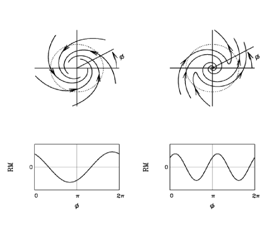 |
different possibilities (Tosa & Fujimoto 1978; Sofue, Fujimoto, & Wielebinski 1986). For example, one can plot RM as a function of the azimuthal angle at fixed physical distance from the galactic center. The result will be a single (double) periodic distribution for a pure axisymmetric (bisymmetric) field configuration. The RM- method has a number of weaknesses as outlined in Ruzmaikin, Sokoloff, Shukurov, & Beck (1990) and Sokoloff, Shukurov, & Krause (1992). In particular, the method has difficulty disentangling a magnetic field configuration that consists of a superposition of different modes. In addition, determination of the RM is plagued by the “ degeneracy” and therefore observations at a number of wavelengths is required. An alternative is to consider the polarization angle as a function of . and model as a Fourier series: . The coefficients and then provide a picture of the azimuthal structure of the field. Of course, if an estimate of the field strength is desired, multiwavelength observations are again required (Ruzmaikin, Sokoloff, Shukurov, & Beck 1990; Sokoloff, Shukurov, & Krause 1992).
In M31, both and methods suggest strongly that the regular magnetic field in the outer parts of the galaxy (outside the synchroton emission ring) is described well by an axisymmetric field. Inside the ring, the field is more complicated and appears to have a significant admixture of either or modes (Ruzmaikin, Sokoloff, Shukurov, & Beck 1990). These higher harmonics may be an indication that the dynamo is modulated by the two-arm spiral structure observed in this region of the galaxy. The polarized synchrotron emissivity along the ring may provide a further clue as to the structure of the magnetic field. The emissivity is highly asymmetric — in general much stronger along the minor axis of the galaxy. Urbanik, Otmianowska-Mazur, & Beck (1994) suggested that this pattern in emission are better explained by a superposition of helical flux tubes that wind along the axis of the ring rather than a pure azimuthal field. (For a further discussion of helical flux tubes in the context of the -dynamo see Donner & Brandenburg 1990).
Field configurations in disk galaxies can also be classified according to their symmetry properties with respect to reflections about the central plane of the galaxy. Symmetric, or even parity field configurations are labeled Sm where, as before, is the azimuthal mode number. Antisymmetric or odd parity solutions are labelled . Thus as S0 field configuration is axisymmetric (about the spin axis) and symmetric about the equatorial plane. An A0 configuration is also axisymmetric but is antisymmetric with respect to the equatorial plane. As shown in Figure 2, the poloidal component of a symmetric (antisymmetric) field configuration has a quadruple (dipole) structure.

The parity of a field configuration in a spiral galaxy is extremely difficult to determine. Indeed, evidence in favor of one or the other type of symmetry has been weak at best and generally inconclusive (Krause & Beck 1998). One carefully studied galaxy is the Milky Way where the magnetic field has been mapped from the RMs of galactic and extragalactic radio sources. An analysis by Han, Manchester, Berkhuijsen, & Beck (1997) of over 500 extragalactic objects suggests that the field configuration in the inner regions of the Galaxy is antisymmetric about its midplane. On the other hand the analysis by Frick et al. (2001) indicates that the field in the solar neighborhood is symmetric. Evidently, the parity of the field configuration can change from one part of a galaxy to another. A second well-studied case is M31 where an analysis of the RM across its disk suggests that the magnetic field is symmetric about the equatorial plane, i.e., an even-parity axisymmetric (S0) configuration (Han, Beck, & Berkhuijsen 1998).
Among S0-type galaxies, there is an additional question as to the direction of the magnetic field, namely whether the field is oriented inward toward the center of the galaxy or outward (Krause & Beck 1998). The two possibilities can be distinguished by comparing the sign of the RM (as a function of position on the disk) with velocity field data. Krause & Beck (1998) point out that in four of five galaxies where the field is believed to be axisymmetric, those fields appear to be directed inward. This result is somewhat surprising given that a magnetic dynamo shows no preference for one type of orientation over the other. It would be premature to draw conclusions based on such a small sample. Nevertheless, if, as new data becomes available, a preference is found for inward over outward directed fields (or more realistically, a preference for galaxies that are in the same region of space to have the same orientation), it would reveal a preference in initial conditions and therefore speak directly to the question of seed fields.
III.2.3 Connection with Spiral Structure
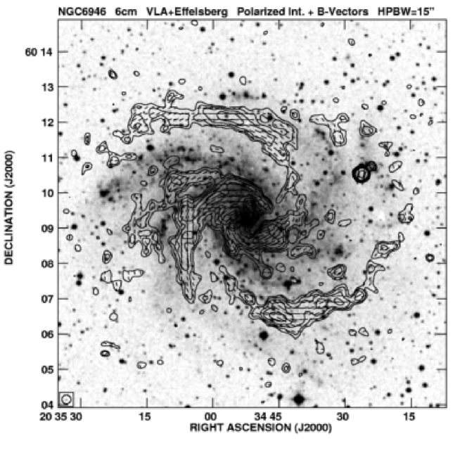
Often, the spiral magnetic structures detected in disk galaxies appear to be closely associated with the material spiral arms. A possible connection between magnetic and optical spiral structure was first noticed in observations of M83 (Sukumar & Allen 1989), IC 342 and M81 (Krause, Hummel, & Beck 1989a, 1989b). A particularly striking example of magnetic spiral structure is found in the galaxy NGC 6946, as shown in Figure 3 (Beck & Hoernes 1995; Frick et al. 2000). In each case, the map of linearly polarized synchrotron emission shows clear evidence for spiral magnetic structures across the galactic disk. The magnetic field in IC 342 appears to be an inwardly-directed axisymmetric spiral while the field in M81 is more suggestive of a bisymmetric configuration (Sofue, Takano, & Fujimoto 1980; Krause, Hummel, & Beck 1989a, 1989b; Krause 1990). In many cases, magnetic spiral arms are strongest in the regions between the optical spiral arms but otherwise share the properties (e.g., pitch angle) of their optical counterparts. These observations suggest that either the dynamo is more efficient in the interarm regions or that magnetic fields are disrupted in the material arms. For example, Mestel & Subramanian (1991, 1993) proposed that the -effect of the standard dynamo contains a non-axisymmetric contribution whose configuration is similar to that of the material spiral arms. The justification comes from one version of spiral arm theory in which the material arm generates a spiral shock in the interstellar gas. The jump in vorticity in the shock may yield an enhanced -effect with a spiral structure. Further theoretical ideas along these lines were developed by Shukurov (1998) and a variety of numerical simulations which purport to include nonaxisymmetric turbulence have been able to reproduce the magnetic spiral structures found in disk galaxies (Rohde & Elstner 1998; Rohde, Beck, & Elstner 1999; Elstner, Otmianowska-Mazur, von Linden, & Urbanik 2000). Along somewhat different lines, Fan & Lou (1996) attempted to explain spiral magnetic arms in terms of both slow and fast magnetohydrodynamic waves.
Recently, Beck et al. (1999) discovered magnetic fields in the barred galaxy NGC 1097. Models of barred galaxies predict that gas in the region of the bar is channeled by shocks along highly non-circular orbits. The magnetic field in the bar region appears to be aligned with theoretical streamlines suggesting that the field is mostly frozen into the gas flow in contrast with what is expected for a dynamo-generated field. The implication is that a dynamo is required to generate new field but that inside the bar simple stretching by the gas flow is the dominant process (see Moss et al. 2001).
III.2.4 Halo Fields
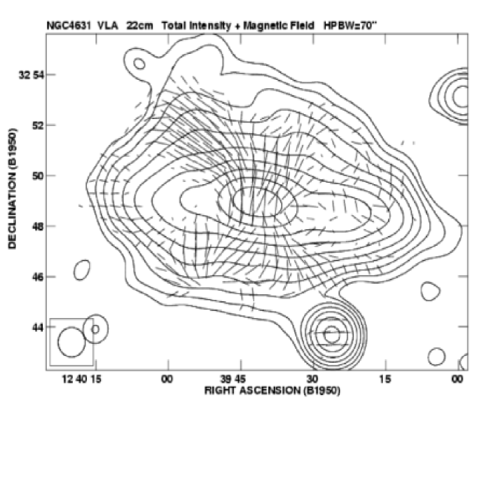
Radio observations of magnetic fields in edge-on spiral galaxies suggest that in most cases the dominant component of the magnetic field is parallel to the disk plane (Dumke, Krause, Wielebinski, & Klein 1995). However, for at least some galaxies, magnetic fields are found to extend well away from the disk plane and have strong vertical components. Hummel, Beck, and Dahlem (1991) mapped two such galaxies, NGC 4631 and NGC 891, in linearly polarized radio emission and found fields with strength and respectively with scale heights . The fields in these two galaxies have rather different characteristics: In NGC 4631 (Figure 4), numerous prominent radio spurs are found throughout the halo. In all cases where the magnetic field can be determined, the field follows these spurs (Golla & Hummel 1994). (Recent observations by Tüllmann et al. (2000) revealed similar structures in the edge-on spiral NGC 5775.) Moreover, the large-scale structure of the field is consistent with that of a dipole configuration (anti-symmetric about the galactic plane) as in the bottom panel of Figure 2. The field in NGC 891 is more disorganized, that is, only ordered in small regions with no global structure evident.
Magnetic fields are but one component of the ISM found in the halos of spiral galaxies. Gas (which exists in many different phases), stars, cosmic rays, and interstellar dust, are also present. Moreover, the disk and halo couple as material flows out from the disk and into the halo only to eventually fall back completing a complex circulation of matter (see, for example, Dahlem 1997). At present, it is not clear whether halo fields are the result of dynamo action in the halo or alternatively, fields produced in the disk and carried into the halo by galactic winds or magnetic buoyancy (see Section IV.G).
III.2.5 Far Infrared-Radio Continuum Correlation
An observation that may shed light on the origin and evolution of galactic magnetic fields is the correlation between galactic far infrared (FIR) emission and radio continuum emission. This correlation was first discussed by Dickey & Salpeter (1984) and de Jong, Klein, Wielebinski, & Wunderlich (1985). It is valid for various types of galaxies including spirals, irregulars, and cluster galaxies and has been established for over four orders of magnitude in luminosity (see Niklas & Beck (1997) and references therein). The correlation is intriguing because the FIR and radio continuum emissions are so different. The former is thermal and presumably related to the star formation rate (SFR). The latter is mostly nonthermal and produced by relativistic electrons in a magnetic field. Various proposals to explain this correlation have been proposed (For a review, see Niklas & Beck (1997).) Perhaps the most appealing explanation is that both the magnetic field strength and the star formation rate depend strongly on the volume density of cool gas (Niklas & Beck 1997). Magnetic field lines are anchored in gas clouds (Parker 1966) and therefore a high number density of clouds implies a high density of magnetic field lines. Likewise, there are strong arguments in favor of a correlation between gas density and the SFR of the form SFR (Schmidt 1959). With an index , taken from survey data of thermal radio emission (assumed to be an indicator of the SFR), where able to provide a self-consistent picture of the FIR and radio continuum correlation.
III.3 Elliptical and Irregular Galaxies
Magnetic fields are ubiquitous in elliptical galaxies though they are difficult to observe because of the paucity of relativistic electrons. Nevertheless, their presence is revealed through observations of synchrotron emission. In addition, Faraday rotation has been observed in the polarized radio emission of background objects. One example is that of a gravitationally lensed quasar where the two quasar images have rotation measures that differ by (Greenfield, Roberts, & Burke 1985). The conjecture is that light for one of the images passes through a giant cD elliptical galaxy whose magnetic field is responsible for the observed Faraday rotation. A more detailed review of the observational literature can be found in Moss & Shukurov (1996). These authors stress that while the evidence for microgauss fields in ellipticals is strong, there are no positive detections of polarized synchrotron emission or any other manifestation of a regular magnetic field. Thus, while the inferred field strengths are comparable to those found in spiral galaxies, the coherence scale for these fields is much smaller than the scale of the galaxy itself.
Recently, magnetic fields were observed in the dwarf irregular galaxy NGC 4449. The mass of this galaxy is an order of magnitude lower than that of the typical spiral and shows only weak signs of global rotation. Nevertheless, the regular magnetic field is measured to be , comparable to that found in spirals (Chyzy et al. 2000). Large domains of non-zero Faraday rotation indicate that the regular field is coherent on the scale of the galaxy. This field appears to be composed of two distinct components. First, there is a magnetized ring in radius in which clear evidence for a regular spiral magnetic field is found. This structure is reminiscent of the one found in M31. Second, there are radial “fans” – coherent magnetic structures that extend outward from the central star forming region. Both of these components may be explained by dynamo action though the latter may also be due to outflows from the galactic center which can stretch magnetic field lines.
III.4 Galaxy Clusters
Galaxy clusters are the largest non-linear systems in the Universe. X-ray observations indicate that they are filled with a tenuous hot plasma while radio emission and RM data reveal the presence of magnetic fields. Clusters are therefore an ideal laboratory to test theories for the origin of extragalactic magnetic fields (see, for example, Kim, Tribble, & Kronberg 1991; Tribble 1993).
Data from the Einstein, ROSAT, Chandra, and XMM-Newton observatories provide a detailed picture of rich galaxy clusters. The intracluster medium is filled with a plasma of temperature that emits X-rays with energies . Rich clusters appear to be in approximate hydrostatic equilibrium with virial velocities (see, for example, Sarazin 1986). In some cluster cores, the cooling time for the plasma due to the observed X-ray emission is short relative to the dynamical time. As the gas cools, it is compressed and flows inward under the combined action of gravity and the thermal pressure of the hot outer gas (Fabian, Nulsen, & Canizares 1984). These cooling flows are found in elliptical galaxies and groups as well as clusters. The primary evidence for cooling flows comes from X-ray observations. In particular, a sharp peak in the X-ray surface brightness distribution is taken as evidence for a cooling flow since it implies that the gas density is rising steeply towards the cluster center (see, for example, Fabian 1994).
A small fraction of rich clusters have observable radio halos. Hanisch (1982) examined data from four well-documented examples and found that radio-halo clusters share a number of properties — principally, a large homogeneous hot intracluster medium and the absence of a central dominant (cD) galaxy. He concluded that radio halos are short-lived phenomena, symptoms of a transient state in the lifetime of a cluster.
Magnetic fields appear to exist in galaxy clusters regardless of whether there is evidence of cooling flows or extended radio emission. Taylor, Barton, & Ge (1994), working from the all-sky X-ray sample of galaxies of Edge et al. (1992), concluded that over half of all cooling flow clusters have and a significant number have . Furthermore, they found a direct correlation between the cooling flow rate and the observed RM. Estimates of the regular magnetic field strength for clusters in their sample range from .
Evidence for magnetic fields in radio-halo clusters is equally strong. Kim et al. (1990) determined the RM for 18 sources behind the Coma cluster and derived an intracluster field strength of where , a model parameter, is the typical scale over which the field reverses direction. Unfortunately, for most clusters, there are no more than a few radio sources strong enough to yield RM measurements. To circumvent this problem, several authors, beginning with Lawler & Dennison (1982), employed a statistical approach by combining data from numerous clusters. For example, Kim, Tribble, & Kronberg (1991) used data from clusters (including radio-halo and cooling-flow clusters), to plot the RM of background radio sources as a function of their impact parameter from the respective cluster center. The dispersion in RMs rises from a background level of to near the cluster center revealing the presence of magnetic fields in most, if not all, of the clusters in the sample. Recently, Clarke, Kronberg, & Böhringer (2001) completed a similar study of 16 “normal” Abell clusters selected to be free of widespread cooling flows and strong radio halos. Once again, the dispersion in RM is found to increase dramatically at low impact parameters indicating strong () magnetic fields on scales of order .
Radio emission is of course produced by relativistic electrons spiralling along magnetic field lines. These same electrons can Compton scatter CMB photons producing a non-thermal spectrum of X-rays and -rays. At high energies, these Compton photons can dominate the thermal X-ray emission of the cluster (e.g., Rephaeli 1979). In contrast to synchrotron emission, the flux of the Compton X-rays is a decreasing function of — for the power-law electron distribution in Eq. (23) — so that an upper limit on the non-thermal X-ray flux translates to a lower limit on the magnetic field strength in the cluster. Using this method, Rephaeli & Gruber (1988) found a lower limit for several Abell clusters in agreement with the positive detections described above.
III.5 Extracluster Fields
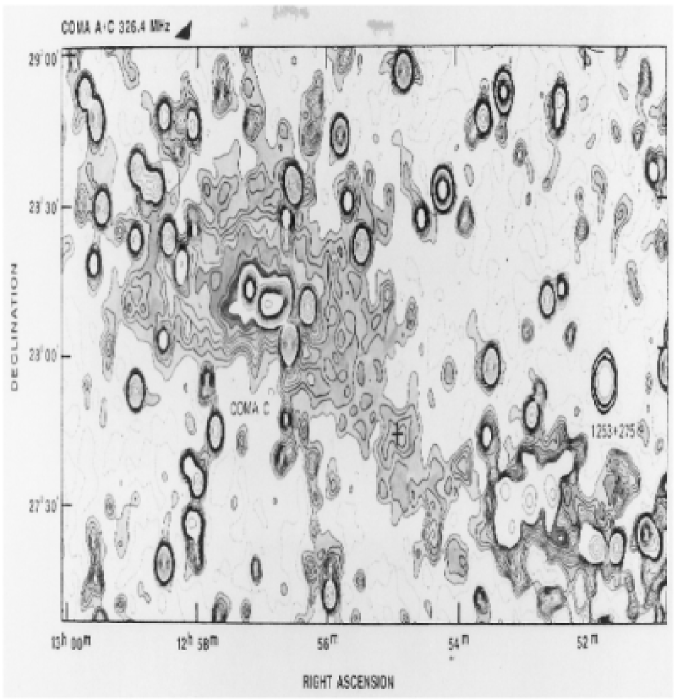
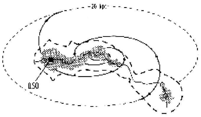
There are hints that magnetic fields exist on supercluster scales. Kim et al. (1989) detected faint radio emission in the region between the Coma cluster and the cluster Abell 1367. These two clusters are apart and define the plane of the Coma supercluster. Kim et al. (1989) observed a portion of the supercluster plane using the Westerbork Synthesis Radio Telescope. They subtracted emission from discrete sources such as extended radio galaxies and found, in the residual map, evidence of a ‘bridge’ in radio emission (Figure 5). The size of the ‘bridge’ was estimated to be in projection where is the Hubble constant in units of . They concluded that the ‘bridge’ was a feature of the magnetic field of the Coma-Abell 1367 supercluster with a strength, derived from minimum energy arguments, of .
Indirect evidence of extracluster magnetic fields may exist in radio observations by Ensslin et al. (2001) of the giant radio galaxy NGC 315. New images reveal significant asymmetries and peculiarities in this galaxy. These features can be attributed to the motion of the galaxy through a cosmological shock wave times the dimension of a typical cluster. Polarization of the radio emission suggests the presence of a very-large scale magnetic field associated with the shock.
III.6 Galactic Magnetic Fields at Intermediate Redshifts
Evidence of magnetic fields in galaxies at even moderate redshifts poses a serious challenge to the galactic dynamo hypothesis since it would imply that there is limited time available for field amplification. At present, the most convincing observations of galactic magnetic fields at intermediate redshifts come from RM studies of radio galaxies and quasars. Kronberg, Perry, & Zukowski (1992) obtained an RM map of the radio jet associated with the quasar PKS 1229-121. This quasar is known to have a prominent absorption feature presumably due to an intervening object at . (The intervener has not been imaged optically). Observations indicate that the RM changes sign along the “ridge line” of the jet in a quasi-oscillatory manner. One plausible explanation is that the intervener is a spiral galaxy with a bisymmetric magnetic field as illustrated in Figure 6. Alternatively, the field in the intervening galaxy might be axisymmetric with reversals along the radial direction. (A configuration of this type has been suggested for the Milky Way (see, for example, Poedz, Shukurov, & Sokoloff 1993).)
Athreya et al. (1998) studied 15 high redshift () radio galaxies at multiple frequencies in polarized radio emission and found significant RMs in almost all of them with several of the objects in the sample having . The highest RM in the sample is for the galaxy 1138-262. RMs of this magnitude require microgauss fields that are coherent over several .
III.7 Cosmological Magnetic Fields
A truly cosmological magnetic field is one that cannot be associated with collapsing or virialized structures. Cosmological magnetic fields can include those that exist prior to the epoch of galaxy formation as well as those that are coherent on scales greater than the scale of the largest known structures in the Universe, i.e., . In the extreme, one can imagine a field that is essentially uniform across our Hubble volume. At present, we do not know whether cosmological magnetic fields exist.
Observations of magnetic fields in the Coma supercluster and in redshift radio galaxies hint at the existence of widespread cosmological fields and lend credence to the hypothesis that primordial fields, amplified by the collapse of a protogalaxy (but not necessarily by dynamo action), become the microgauss fields observed in present-day galaxies and clusters. (An even bolder proposal is that magnetic fields play an essential role in galaxy formation. See, for example, Wasserman 1978; Kim, Olinto, & Rosner 1996.) The structure associated with the magnetic ‘bridge’ in the Coma supercluster (Kim et al. 1989) is dynamically young so that there has been little time for dynamo processes to operate. The observations by Athreya et al. (1998) and, to a lesser extent, Kronberg, Perry, & Zukowski (1992), imply that a similar problem exists on galactic scales. Interest in the primordial field hypothesis has also been fueled by challenges to the standard dynamo scenario.
A detection of sufficiently strong cosmological fields would provide tremendous support to the primordial field hypothesis and at the same time open a new observational window to the early Universe. Moreover, since very weak cosmological fields can act as seeds for the galactic dynamo the discovery of even the tiniest cosmological field would help complete the dynamo paradigm.
For the time being, we must settle for limits on the strength of cosmological fields. Constraints have been derived from Faraday rotation studies of high-redshift sources, anisotropy measurements of the CMB, and predictions of light element abundances from big bang nucleosynthesis (BBN).
III.7.1 Faraday Rotation due to a Cosmological Field
Faraday rotation of radio emission from high redshift sources can be used to study cosmological magnetic fields. For a source at a cosmological distance , the rotation measure is given by the generalization of Eq. (30) appropriate to an expanding Universe:
| (33) |
The factor of accounts for the redshift of the electromagnetic waves as they propagate from source to observer. We consider the contribution to this integral from cosmological magnetic fields. If the magnetic field and electron density are homogeneous across our Hubble volume, an all-sky RM map will have a dipole component (Sofue, Fujimoto, Kawabata 1968; Brecher & Blumenthal 1970; Vallée 1975; Kronberg 1977; Kronberg & Simard-Normandin 1976; Vallée 1990). The amplitude of this effect depends on the evolution of and . The simplest assumption is that the comoving magnetic flux and comoving electron number density are constant, i.e., and . The cosmological component of the RM is then
| (34) |
where is the angle between the source and the magnetic field,
| (35) |
and
| (36) |
In Figure 7, we plot and as a function of for selected cosmological models. The path length to a source and hence the cosmological contribution to the RM are increasing functions of , as is evident in Figure 7. In addition, for fixed , the is greater in low- models than in the Einstein-de Sitter model, a reflection of the fact that the path length per unit redshift interval is greater in those models.

Eqs. (34)-(36), together with RM data for high-redshift galaxies and quasars, can be used to constrain the strength of Hubble-scale magnetic fields. The difficulty is that the source and Galaxy contributions to the RM are unknown. (Indeed, Sofue, Fujimoto, and Kawabata (1968) reported a positive detection of a cosmological field, a result which was refuted by subsequent studies.) By and large, the Galactic contribution is and in general decreases with increasing angle relative to the Galactic plane. However, Kronberg and Simard-Normandin (1976) found that even at high Galactic latitude, some objects have . In particular, the high Galactic latitude subsample that they considered was evidently composed of two distinct populations, one with and another with . (A similar decomposition is not possible at low Galactic latitudes where the contribution to the RM from the Galactic magnetic field is stronger. However, the RM sky at low Galactic latitudes does reveal a wealth of structure in the Galactic magnetic field (see, for example, Duncan, Reich, Reich, & Fürst (1999) and Gaensler et al. (2001).) This observation suggests that the best opportunity to constrain Hubble-scale magnetic fields comes from the high Galactic latitude, low-RM subsample. For example, Vallée (1990) tested for an RM dipole in a sample of 309 galaxies and quasars. The galaxies in this sample extended to though most of the objects were at . Vallée derived an upper limit to of about , corresponding to an upper limit of on the strength of the uniform component of a cosmological magnetic field.
If either the electron density or magnetic field vary on scales less than the Hubble distance, the pattern of the cosmological contribution to the RM across the sky will be more complicated than a simple dipole. Indeed, if variations in and occur on scales much less than , a typical photon from an extragalactic source will pass through numerous “Faraday screens”. In this case, the average cosmological RM over the sky will be zero. However, , the variance of RM, will increase with . Kronberg and Perry (1982) considered a simple model in which clouds of uniform electron density and magnetic field are scattered at random throughout the Universe. The rotation measure associated with a single cloud at a redshift is given by
| (37) |
where and are the cloud radius and electron column density respectively. For simplicity, all clouds at a given redshift are assumed to share the same physical characteristics. The contribution to from clouds between and can be written
| (38) |
where
| (39) |
and is the number density of clouds in the Universe. Kronberg & Perry (1982) estimated under the assumption that the comoving number density of clouds, as well as their comoving size, electron density, and magnetic flux are constant, i.e., and . The expression for then becomes
| (40) |
where is an integral similar to the one in Eq. (35).
The Kronberg-Perry model was motivated by spectroscopic observations of QSOs which reveal countless hydrogen absorption lines spread out in frequency by the expansion of the Universe. This dense series of lines, known as the Ly-forest, implies that there are a large number of neutral hydrogen clouds at cosmological distances. Kronberg & Perry (1982) selected model parameters motivated by the Ly-cloud observations of Sargent et al. (1980), specifically, , , and . For these parameters, the estimate for is disappointingly small. For example, in a spatially flat, model, . Detection above the “noise” of the galactic contribution requires or equivalently . A magnetic field of this strength would have been well above the equipartition strength for the clouds.
Clearly, the limits derived from RM data depend on the model one assumes for the Ly-clouds. Recently, Blasi, Burles, & Olinto (1999) suggested that the conclusions of Kronberg & Perry (1982) were overly pessimistic. Their analysis was motivated by a model for the intergalactic medium by Bi & Davidsen (1997) and Coles & Jones (1991) in which the Universe is divided into cells of uniform electron density while the magnetic field is parametrized by its coherence length and mean field strength. Random lines of sight are simulated for various model universes. The results suggest that a detectable variance in RM is possible for magnetic fields as low as . The enhanced sensitivity relative to the Kronberg & Perry (1982) observations is primarily due to the larger filling factor assumed for the clouds: The clouds in Kronberg & Perry (1982) have a filling factor of order while those of Blasi, Burles, and Olinto (1999) have a filling factor of .
Further improvements in the use of Faraday rotation to probe cosmological magnetic fields may be achieved by looking for correlations in RM (Kolatt, 1998). The correlation function for the RM from sources with an angular separation that is small compared to the angular size of the clouds increases as , i.e., , where is the average number of clouds along the line of sight (Kolatt 1998). By contrast, increases linearly with , i.e., . Thus, the signal in a correlation map can be enhanced over the signal by an order of magnitude or more. Moreover, in a correlation map, the “noise” from the Galaxy is reduced. Finally, the correlation method can provide information about the power spectrum of cosmological fields and the statistical properties of the clouds.
A different approach was taken by Kronberg & Perry (1982) who argued that since the due to Ly-clouds is small, a large observed must be due to either gas intrinsic to the QSO or to a few rare gas clouds (e.g., a gaseous galactic halo) along the QSO line of sight. The implication is that the distribution of in a sample of QSOs will be highly nongaussian (i.e., large for a subset of QSOs but small for many if not most of the others) and correlated statistically with redshift and with the presence of damped Ly-systems. Kronberg & Perry (1982), Welter, Perry, & Kronberg (1984) and Wolfe, Lanzetta, & Oren (1992) all reported evidence for these trends in RM data from QSO surveys. Wolfe, Lanzetta, & Oren (1992), for example, found that in a sample of 116 QSOs, the 5 with known damped Ly-systems had large as compared with (i.e., ) of those in the rest of the sample. However Perry, Watson, & Kronberg (1993) argued that the case for strong magnetic fields in damped Ly-systems is unproven, the most serious problems in the Wolfe, Lanzetta, & Oren (1992) analysis arising from the sparsity and heterogeneous nature of the data. In particular, since electron densities can vary by at least an order of magnitude, a case by case analysis is required. Moreover, a subsequent study by Oren & Wolfe (1995) of an even larger data set found no evidence for magnetic fields in damped Ly-systems.
III.7.2 Evolution of Magnetic Fields in the Early Universe
Limits on cosmological magnetic fields from CMB observations and BBN constraints are discussed in the two subsections that follow. These limits are relevant to models in which magnetic fields arise in the very early Universe (see Section V.C). In this subsection, we discuss briefly the pre-recombination evolution of magnetic fields.
During most of the radiation-dominated era, magnetic fields are frozen into the cosmic plasma. So long as this is the case, a magnetic field, coherent on a scale at a time , will evolve, by a later time according to the relation
| (41) |
Jedamzik, Katalinic, & Olinto (1998) pointed out that at certain epochs in the early Universe, magnetic field energy is converted into heat in a process analogous to Silk damping (Silk 1968). In particular, at recombination, the photon mean free path and hence radiation diffusion length scale becomes large and magnetic field energy is dissipated. The damping of different MHD modes — Alfvén, fast magnetosonic, and slow magnetosonic — is a complex problem and the interested reader is referred to Jedamzik, Katalinic, & Olinto (1998). In short, modes whose wavelength is larger than the Silk damping scale at decoupling (comoving length ) are unaffected while damping below the Silk scale depends on the type of mode and the strength of the magnetic field.
III.7.3 Limits from CMB Anisotropy Measurements
A magnetic field, present at decoupling () and homogeneous on scales larger than the horizon at that time, causes the Universe to expand at different rates in different directions. Since anisotropic expansion of this type distorts the CMB, measurements of the CMB angular power spectrum imply limits on the cosmological magnetic fields (Zel’dovich & Novikov 1983; Madsen 1989; Barrow, Ferreira, & Silk 1997).
The influence of large-scale magnetic fields on the CMB is easy to understand (see, for example, Madsen 1989). Consider a universe that is homogeneous and anisotropic where the isotropy is broken by a magnetic field that is unidirectional but spatially homogeneous. Expansion of the spacetime along the direction of the field stretches the field lines and must therefore do work against magnetic tension. Conversely, expansion orthogonal to the direction of the field is aided by magnetic pressure. Thus, the Universe expands more slowly along the direction of the field and hence the cosmological redshift of an object in this direction is reduced relative to what it would be in a universe in which .
Zel’dovich & Novikov (1983) and Madsen (1989) considered a spatially flat model universe that contains a homogeneous magnetic field. The spacetime of this model is Bianchi type I, the simplest of the nine homogeneous and anisotropic three-dimensional metrics known collectively as the Bianchi spacetimes. The analysis is easily extended to open homogeneous anisotropic spacetimes (i.e., universes with negative spatial curvature), known as Bianchi type V (Barrow, Ferreira, & Silk 1997). In the spatially flat case, the model is described by two dimensionless functions of time. The first is the ratio of the energy density in the field relative to the energy density in matter:
| (42) |
The second function is the difference of expansion rates orthogonal to and along the field divided by the Hubble parameter. The fact that the angular anisotropy of the CMB is small on all angular scales implies that the both of these functions are small. Madsen (1989) found that to a good approximation
| (43) |
where the subscript ‘d’ refers to the decoupling epoch. If we assume that the field is frozen into the plasma, then and . By definition . The constraint implied by Eq. (43) can therefore be written
| (52) | |||||
| (61) |
While this expression was derived assuming a pure Bianchi type I model (i.e., homogeneous on scales larger than the present day horizon) the main contribution to the limit comes from the expansion rate at decoupling and therefore the result should be valid for scales as small as the scale of the horizon at decoupling.
Barrow, Ferreira, & Silk (1997) carried out a more sophisticated statistical analysis based on the 4-year Cosmic Background Explorer (COBE) data for angular anisotropy and derived the following limit for primordial fields that are coherent on scales larger than the present horizon:
| (62) |
Measurements of the CMB angular anisotropy spectrum now extend to scales times smaller than the present-day horizon (Balbi et al. 2000; Melchiorri et al. 2000; Pryke et al. 2001). These measurements imply that for fields with a comoving coherence length their strength, when scaled via Eq. (41) to the present epoch, must be (Durrer, Kahniashvili, & Yates 1998; Subramanian & Barrow 1998). Future observations should be able to detect or limit magnetic fields on even smaller scales. However, the interpretation of any limit placed on magnetic fields below the Silk scale is complicated by the fact that such fields are damped by photon diffusion (Jedamzik, Katalinic, & Olinto 1998; Subramanian & Barrow 1998). If a particular MHD mode is efficiently damped prior to decoupling, then any limit on its amplitude is essentially useless.
Jedamzik, Katalinic, & Olinto (2000) pointed out that as MHD modes are damped, they heat the baryon-photon fluid. Since this process occurs close to the decoupling epoch, it leads to a distortion of the CMB spectrum. Using data from the COBE/FIRAS experiment (Fixen 1996), they derived a limit on the magnetic field strength of (scaled to the present epoch) between comoving scales and .
The existence of a magnetic field at decoupling may induce a measurable Faraday rotation in the polarization signal of the CMB. Kosowsky & Loeb (1996) showed that a primordial field with strength corresponding to a present-day value of induces a rotation at and a strategy to measure this effect in future CMB experiments was suggested.
III.7.4 Constraints from Big Bang Nucleosynthesis
Big bang nucleosynthesis (BBN) provides the earliest quantitative test of the standard cosmological model (see, for example, Schramm & Turner 1998; Olive, Steigman, & Walker 2000). BBN took place between and after the Big Bang and is responsible for most of the 4He, 3He, D, and 7Li in the Universe. Numerical calculations yield detailed predictions of the abundances of these elements which can be compared to observational data. Over the years, discrepancies between theory and observation have come and gone. Nevertheless, at present, BBN must be counted as an unqualified success of the Big Bang paradigm.
Magnetic fields can alter the predictions of BBN. Thus, the success of BBN — specifically, the agreement between theoretical predictions and observations of the light element abundances — imply limits on the strength of primordial fields. Limits of this type were first proposed by Greenstein (1969) and O’Connell & Matese (1970). They identified the two primary effects of magnetic fields on BBN: (i) nuclear reaction rates change in the presence of strong magnetic fields, and (ii) the magnetic energy density leads to an increase cosmological expansion rate. During the 1990’s, detailed calculations were carried out by numerous groups including Cheng, Schramm, & Truran (1994), Grasso & Rubenstein (1996), Kernan, Starkman, & Vachaspati (1996), and Cheng, Olinto, Schramm, & Truran (1996). Though the results from these groups did not always agree (see, for example, Kernen, Starkman, & Vachaspati (1997). The general concensus is that the dominant effect comes from the change in the expansion rate due to magnetic field energy.
The effects of a magnetic field on BBN can be understood in terms of the change they induce in the neutron fraction. For example, a magnetic field affects the neutron fraction by altering the electron density of states. In a uniform magnetic field, the motion of an electron can be decomposed into linear motion along the direction of the field and circular motion in the plane perpendicular to the field. According to the principles of quantum mechanics, the energy associated with the circular motion is quantized and the total energy of the particle can be written
| (63) |
where is the quantum number for the different energy eigenstates known as Landau levels (Landau & Lifshitz ) which are important for field strengths . The (partial) quantization of the electron energy implied by Eq. (63) therefore changes the density of states of the electrons which in turn affects processes such as neutron decay where it leads to an increase in the decay rate.
If the only effect of the magnetic field was to increase nuclear reaction rates, it would lead to a decrease in the number of neutrons at the time of BBN and hence a decrease in the abundance. However, a magnetic field also contributes to the energy density of the Universe and therefore alters the time-temperature relationship. If the correlation length of the field is greater than the horizon scale, the field causes the Universe to expand anisotropically. On the other hand, a field whose correlation scale is much smaller than the horizon can be treated as a homogeneous and isotropic component of the total energy density of the Universe. In either case, the magnetic field increases the overall expansion rate thus decreasing the time over which nucleosynthesis can occur and in particular the time over which neutrons can decay. The net result is an increase in the abundance. The helium abundance is fixed when the age of the Universe is and the temperature is . At this time, the energy density of the Universe is which is comparable to the energy density in a magnetic field. The magnetic field must be somewhat less than this value so as not to spoil the predictions of BBN. If one assumes that the magnetic field scales according to Eq.(41) then this leads to the following constraint on the magnetic field at the present epoch .
III.7.5 Intergalactic Magnetic Fields and High Energy Cosmic Rays
Cosmic rays are relativistic particles (primarily electrons and protons with a small admixture of light nuclei and antiprotons) that propagate through the Galaxy with energies ranging from (Hillas 1998). Their energy spectrum is characterized by a power law up to the ‘knee’ (), a slightly steeper power law between the knee and the ‘ankle’, (), and a flattened distribution (the ultrahigh energy cosmic rays or UHECRs) above the ankle. The origin of the UHECRs is a mystery. Circumstantial evidence suggests that these particles are created outside the Galaxy but within . Since the gyrosynchrotron radius for a particle in the Galactic magnetic field with is larger than the Galaxy, if UHECRs originated in the Galaxy, the arrival direction would point back to the source. However, to date, no sources have been identified. On the other hand, protons with energies above interact with CMB photons producing pions over a mean free path of order . Therefore if most UHECRs originated at cosmological distances, their energy spectrum would show a distinct drop known as the GZK cut-off (Greisen, 1966; Zatsepin & V. A. Kuzmin 1966). The absence of such a cut-off implies that UHECRs are produced within .
A number of authors have considered the fate of UHECRs that are produced in the local supercluster (LSC) under the assumption that the LSC is magnetized (Lemoine, et al. 1997; Blasi & Olinto 1999 and references therein). This assumption is reasonable given the detection of magnetic fields in the Coma supercluster (Kim et al. 1989). Blasi & Olinto (1999) found that for a LSC field of cosmic rays with energies below execute a random walk as they travel from source to observer while those above follow a relatively straight path. They argued that the break in the energy spectrum at the ankle is a consequence of the transition from random walk to free-stream propagation. A corollary of this result is that the detection of source counterparts for the particles (or alternatively clustering in the source distribution) would imply a limit on the strength of the magnetic field in the LSC.
The effects of large-scale magnetic fields on UHECRs were also considered by Waxman & Miralda-Escudé (1996). Following Waxman (1995), Vietri (1995) and Milgrom & Usov (1995) they assumed that the same astrophysical objects responsible for -ray bursts also produce UHECRs. The expected rate for -ray bursts within is only per . Since Takeda et al. (1998) observed 7 events above over 8 years a dispersion in arrival times of for cosmic rays produced in a single burst needs to be invoked. Waxman & Miralda-Escudé (1996) proposed that such a dispersion is due to the deflections of UHECRs by a large-scale magnetic field. The induced time delay is estimated to be for a cosmic ray energy of and source at . Magnetic fields have a predictable effect on the angular position and time of flight for cosmic rays of a given energy. Hence, future cosmic ray experiments should be able to determine not only whether or not UHECRs are indeed produced by -ray bursters but whether they are deflected by a large-scale magnetic field on route from source to observer.
Along rather different lines, Plaga (1995) proposed a technique for detecting cosmological magnetic fields at extremely low levels. The idea is to look at the arrival times of -ray photons from cosmological sources (e.g., -ray bursts, flare events in AGN). High energy photons suffer collisions in diffuse extragalactic radiation fields. At -ray energies, the dominant process is electron-positron pair production. The electrons and positrons can then inverse Compton scatter off CMB photons producing high energy photons. An intergalactic magnetic field will deflect the electrons and protons and therefore delay the secondary pulse. In principle, this technique could be able to detect fields as weak as !
IV Galactic and Extragalactic Dynamos
A magnetic dynamo consists of electrically conducting matter moving in a magnetic field in such a way that the induced currents amplify and maintain the original field. The dynamo principle was known in the 1800s though it was Larmor (1919) who first suggested that dynamo processes might be responsible for astrophysical magnetic fields such as those found in the Sun and Earth. Steenbeck, Krause, & Rädler (1966) recognized the importance of helical turbulence for dynamos in stars and planets. Their ideas were soon applied to the problem of galactic magnetic fields by Parker (1971) and Vainshtein & Ruzmaikin (1971, 1972).
Over the years, a standard galactic dynamo model known as the -dynamo has emerged whose essential features are as follows: Turbulent motions in the ISM driven, for example, by stellar winds, supernova explosions, and hydromagnetic instabilities, carry loops of toroidal magnetic field out of the plane of the disk. These loops are twisted into the poloidal plane by the Coriolis effect while toriodal field is regenerated from the poloidal field by differential rotation. The -dynamo can operate in any differentially rotating, turbulent medium and is widely accepted as the primary mechanism for the maintenance of magnetic fields in the Sun (Krause & Rädler 1980; Zel’dovich, Ruzmaikin, & Sokoloff 1983; Ruzmaikin, Sokoloff, & Shukurov 1988a). Its applicability to galaxies has been more controversial and numerous variants and alternative models have been proposed. Nevertheless, the general idea that galactic fields are maintained by differential rotation and small-scale velocity fluctuations is compelling. More speculative is the conjecture that magnetic dynamos act on supergalactic scales. On the other hand, if structure formation proceeds hierarchically, it is plausible that dynamo processes operate sequentially from subgalactic to galactic scales.
An essential feature of a dynamo is its ability to continuously regenerate large-scale magnetic fields. For galaxies, the alternative is that magnetic fields are relics of the early Universe. A magnetic field that permeates the protogalactic medium will be amplified by compression as a galaxy forms and by differential rotation once the disk is fully developed (Hoyle 1958; Piddington 1964, 1972; Kulsrud 1990). The relic field hypothesis has been challenged vigorously by Parker (1973b) and others on the grounds that turbulent diffusion destroys a primordial field on a relatively short timescale. Since these arguments provide a good introduction to the -dynamo, we repeat them below. NB: The dynamo hypothesis does not preclude primordial magnetic fields. To the contrary, while a dynamo can amplify existing fields, the first fields might have been primordial, i.e., created in the very early Universe.
After a brief discussion of the primordial field hypothesis, we review the essentials of mean-field dynamo theory and the standard -dynamo. Particular attention is paid to the assumptions necessary for the development of this model. Some of these assumptions have been challenged as being demonstrably false while others are seen as simply too restrictive. These concerns have led to alternative models for galactic magnetic fields which are discussed at the end of the Section.
IV.1 Primordial Field Hypothesis
Soon after the discovery of galactic magnetic fields, Hoyle (1958) began to contemplate their origin. An astrophysical battery seemed an implausible explanation for galactic fields since the voltage required to drive the requisite currents, , is so enormous. Instead, Hoyle considered a scenario in which magnetic fields are present ab initio in the material that collapses to form a galaxy. Piddington (1964, 1972) championed the primordial field hypothesis and developed models for the structure and evolution of an initially homogeneous field (presumed to be of primordial origin) in a rotating disk galaxy. The primordial field hypothesis hypothesis has been studied recently by Howard & Kulsrud (1997).
The following idealized example illustrates the difficulties with the primordial field hypothesis (Parker 1973b). Consider a differentially rotating disk with angular velocity . (We are using cylindrical () coordinates.) Suppose that at , the magnetic field is uniform and lies in the disk plane. Without loss of generality, we can orient the x-axis to be along the initial direction of the field, i.e., . So long as magnetic diffusion and backreaction effects are negligible, the field at time will be given by
| (64) |
(see Eq. (13)) where . Field lines for an illustrative example are shown in Figure 8. Due to differential rotation, the azimuthal component of the field grows linearly with while gradients in the field grow as . Note that both the initial and final field configurations are bisymmetric. (Alternatively, if the magnetic field is initially oriented along the spin axis of the disk, the field will be axisymmetric but with odd parity about the equatorial plane of the disk, that is, an A0 configuration (see, for example, Ruzmaikin, Shukurov, & Sokoloff 1988a.) Differential rotation, with an axisymmetric velocity field (i.e., independent of ) does not alter the symmetry properties of the field. Roughly speaking, we have where is the disk scale length and . Eventually, magnetic diffusion becomes important with the diffusion timescale, , decreasing with . Linear growth lasts until or equivalently after which the field decays rapidly. In galactic disks, , , and implying a decay time of which is much shorter than the age of a galaxy. (NB: The timescale for the field to decay depends on the structure of the field. If, for example, the field is concentrated in intermittent rope-like structures, the decay time will be much longer than indicated by the estimate above (Subramanian 1998).) Equally problematic is the observation that galactic magnetic fields form, by and large, a loosely wound spiral as in Figure 3 rather than the tightly wound spiral suggested by Figure 8. The implication is that galactic magnetic fields are generated continuously. This argument is similar to the one given in support of the hypothesis that spiral arms are (continuously-generated) density waves propagating through the galactic disk.
These conclusions were challenged recently by Howard & Kulsrud (1997) who investigated the primordial field hypothesis within the context of a simple model for galaxy formation. In particular, they considered a rotating spherical protogalaxy threaded by a constant magnetic field which then collapses to form a disk galaxy. This process leads to amplification of the initial field by several orders of magnitude (see also Lesch & Chiba 1995). The field is then wound up by differential rotation as described above. Howard & Kulsrud (1997) point out that the magnetic field observed in spiral galaxies is an average of the true detailed field. Their contention is that the fine scale structure of the field is that of Figure 8 and only appears as a toroidal azimuthal field because of inadequate resolution.

IV.2 Mean-Field Dynamo Theory
Most discussions of astrophysical dynamos make use of a mean-field approximation to describe the effects of turbulence. In addition, backreaction of the field on the fluid is typically ignored so that the evolution of the field reduces to a purely kinematic problem. Detailed treatments of mean-field dynamo theory can be found in numerous references including Steenbeck, Krause, & Rädler (1966), Moffatt (1978), Parker (1979), Krause & Rädler (1980), Zel’dovich, Ruzmaikin, & Sokoloff 1983, Ruzmaikin, Shukurov, & Sokoloff (1988a), Krause & Wielebinski (1991), Beck et al. (1996) and Kulsrud (1999).
The evolution of a magnetic field in the MHD limit is given by Eq.(6). In a mean-field analysis, we write
| (65) |
where and represent ensemble averages of the magnetic and velocity fields and and are the corresponding small-scale tangled components. The ensemble average of Eq. (7) is
| (66) |
with the residual equation
| (67) |
(We have assumed that molecular diffusion can be neglected.)
The term in Eq. (67) can be eliminated by transforming to the rest frame of the fluid while the terms in this equation are usually ignored. Eq. (67) is then used to eliminate in favor of and in Eq. (66), though this step requires additional assumptions about the statistical properties of the turbulence. The result, which can be derived in a variety of ways (see Ruzmaikin, Shukurov, and Sokoloff 1988a and references therein), is
| (68) |
, the effective electromotive force due to turbulent motions of the magnetic field as it is carried around by the fluid, is often written in terms of two tensors, and :
| (69) |
Explicit expressions for the and tensors can be found in various sources including Ruzmaikin, Shukurov, & Sokoloff (1988a).
The classic example of the -effect is the distortion of a magnetic field line by a localized helical disturbance or cyclonic event (Parker 1970). In the context of a galactic dynamo, we can think of a cyclonic event as a plume of gas rising above the disk and acted upon by differential rotation and the Coriolis effect. Consider a magnetic field configuration that is initially purely toroidal and focus on a single field line at a radius . The velocity field of the plume is assumed to be constant during the “event” () and given by the expression
| (70) |
where we have introduced a local Cartesian coordinate system with and . By design, . The field line of interest is initially . As before, it is traced by particles that are carried along with the fluid. In the absence of rotation, these test particles obey the equation of motion where is the velocity of a test particle as distinct from the fluid velocity field of the plume . The field line after a cyclonic event is shown in Figure 9(a). In a rotating system, it is easiest to follow the evolution of a field line (i.e., the motion of the tracer particles) in a frame rotating with angular velocity . The equation of motion for the particles is then
| (71) |
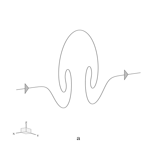 |
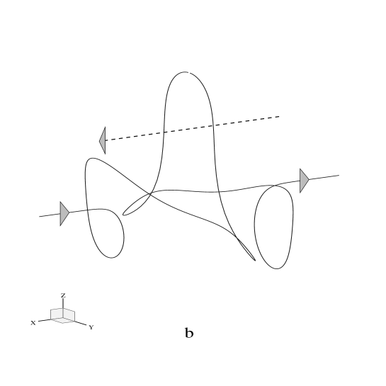 |
where the differential rotation term is not shown explicitly and is ignored in this illustrative example. The second term on the right-hand side of Eq. (71) describes the Coriolis effect which twists the magnetic plume into the poloidal plane (i.e., the yz-plane) as shown in Figure 9(b). Note that the current associated with this loop is anti-parallel to the initial magnetic field line.
Given a specific model for the small-scale velocity field the and tensors can be calculated from first principles (see, for example, Ferrière (1992, 1993, 1998)). However, most calculations make use of ad hoc phenomenological forms for these functions. A simplifying though questionable assumption is that helical turbulence in galactic disks is isotropic. In this case, the and tensors take the form
| (72) |
and
| (73) |
where and are the unit tensor and three-dimensional permutation tensor respectively and is the correlation time of the turbulence. With these expressions for and the dynamo equation becomes
| (74) |
The cyclonic event described above illustrates the dubious nature of the isotropy assumption: Instabilities tend to develop in the direction perpendicular to the disk while vorticity is generated along the spin axis of the galaxy. Moreover, the largest turbulent eddies in the Galaxy are of order in size which is not much smaller than the scale height of the disk. Ferrière (1992, 1993, 1998) has calculated the and tensors for a model in which turbulence is driven by correlated supernova explosions. The results serve as an explicit example of a case where turbulence is decidedly anisotropic. In this model, the -tensor takes the form
| (75) |
The off-diagonal terms describe the convection of magnetic field lines away from the equatorial plane (a “”-term in the induction equation) while the diagonal elements characterize the strength of the -effect along the three coordinate axes. However, while the calculations of Ferrière account for the stretching of magnetic field lines by the expanding supernova shells and concomitant twisting by the Coriolis effect they do not take into account for the -effect due to turbulence that is undoubtedly generated by the expanding shells. Thus, her analysis probably underestimates the strength of the -effect associated with supernovae.
Eq. (68) is the starting point for most discussions of astrophysical dynamos. A self-consistent treatment of the fluid requires an equation of motion for which includes a Lorentz force term describing the backreaction of the field on the fluid. In addition, backreaction may affect the fluctuation fields and thus modifying and . These effects will be discussed below. Here, we assume that backreaction is negligible so that , , and can be specified as model inputs that are independent of . If we further suppose that they are time-independent, the solutions to Eq. (68) will be of the form where the eigenvalue depends on boundary conditions for the field. The solutions of interest are, of course, ones where is real and positive.
IV.3 Disk Dynamos
We consider an axisymmetric differentially-rotating disk galaxy with a large-scale velocity field where . In general and are functions of and with the proviso that . Rotational invariance of the dynamo equations suggests the following Fourier decomposition:
| (76) |
One might guess, and detailed calculations confirm, that the growth rate decreases with increasing so that the fastest growing mode has azimuthal symmetry () (Ruzmaikin, Shukurov, and Sokoloff 1988a). The bisymmetric mode can also be important, though in general this mode is difficult to excite without introducing nonaxisymmetric forms for , , and/or . We will return to this point below and proceed with a discussion of axisymmetric solutions.
In component notation, Eq. (68) becomes
| (77) |
| (78) |
| (79) |
where the overbar and subscript are omitted for the sake of clarity. It is generally assumed that the -terms in the equation for are small compared to the -term (i.e., the toroidal field is generated through the action of differential rotation rather than turbulence). Eqs. (77)-(79) are symmetric under the transformation . Therefore, the solutions will have definite parity with both even and odd parity solutions ( and respectively) possible:
| (80) |
For , and correspond respectively to the even parity () and odd parity () configurations described in Section III.B.2 and shown in Figure 2.
Since the dynamo equations are linear in the fields they admit solutions of the form . Furthermore, for disk-like geometries, variations in the field with respect to will be much greater than those with respect to — in our own Galaxy, the scale height of the disk is a factor of 10 smaller than the scale radius of the disk. This situation suggests a quasi-separation of variables of the form
| (81) |
(see, for example, Ruzmaikin, Shukurov, and Sokoloff 1988a) where labels the different eigenfunctions and eigenvalues . (For a more rigorous discussion of the thin-disk limit in which the Schrödinger-type radial equation (see below) appears as an approximation to the full (integro-differential) see Priklonsky et al. 2000.) depends on parametrically, i.e., no derivatives with respect to appear in the equation for . With this ansatz, the dynamo equations become
| (82) |
| (83) |
and
| (84) |
(Since does not appear in the equations for and we may ignore it at this time. Once and have been determined, may be found from the condition or alternatively by solving the equation.)
Eqs. (82)-(84) can be solved once a complete set of boundary conditions are specified. For simplicity, we assume that the disk is defined by sharp boundaries at and with force-free fields (i.e., ) outside the disk. These conditions imply that and . ( is identically zero in the limit but may be small for a finite disk.)
Eqs. (82) and (83) make clear the essential features of the standard -dynamo. Turbulence via the -effect generates (and ) from while differential rotation regenerates . The sequence of steps for an A0 dynamo is shown schematically in Figure 10. We begin in Figure 10(a) with a pure poloidal dipole-like field. Differential rotation stretches field lines creating toroidal field. This is illustrated in Figure 10(b) where a single field line from Figure 10(a) is shown after it has been acted upon by differential rotation. The field in the equatorial plane is characterized by strong gradients and high magnetic tension. This tension can be relieved either by turbulent diffusion, via the -effect, or by some other process (e.g., magnetic reconnection, see below). The net result is to decouple the toroidal field in the upper and lower hemispheres, as shown in Figure 10(c). Next we assume that cyclonic events occur throughout the disk. The toroidal field is distorted in the vertical direction as in Figure 10(d). The loops of vertical field are then twisted into the poloidal plane by the Coriolis effect (Figure 10(e), see, also Figure 9(b)). Once again, some form of diffusion or dissipation is needed to eliminate magnetic field near the equatorial plane. Provided this occurs, poloidal loops in upper and lower hemispheres can combine to yield a dipole-like field which reinforces the original field (Figure 10(f)).
This example illustrates the importance of diffusion for the dynamo. The and effects twist, shear, and stretch magnetic field lines but do not create new ones. While they can increase the magnetic field energy in the system, they cannot change the net flux through a surface that encloses it. Diffusion eliminates unwanted flux. In the odd parity dynamo of Figure 10, this process occurs in the equatorial region. In an even parity dynamo, diffusion allows flux of the wrong sign to escape by moving to high galactic latitudes.
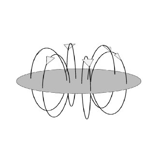 |
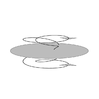 |
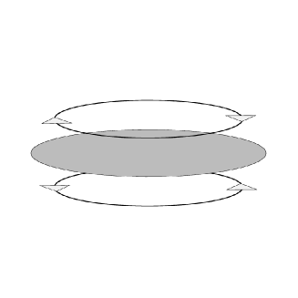 |
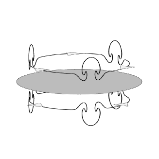 |
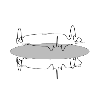 |
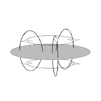 |
The importance of diffusion can be illustrated by considering , the radial flux through the surface at and , the azimuthal flux through a surface at fixed (see, for example, Zel’dovich, Ruzmaikin, & Sokoloff 1983):
| (85) |
From Eq. (77) we find
| (86) |
where contributions from the -term in Eq. (77) vanish because and . With , is constant, i.e., growing mode solutions require .
The equation for is also interesting (Zel’dovich, Ruzmaikin, & Sokoloff 1983). From Eq. (78) we find
| (87) |
For the first term, we integrate by parts and use the condition to find
| (88) |
Thus, with , grows linearly with time, but only if field lines exit the disk through the surface at . If the field lines are confined to the disk, than remains constant even though the energy in the field is increasing due to differential rotation.
Thus, magnetic flux must be expelled from a galaxy inorder for the net large-scale field to grow. Flux expulsion can occur by a number of mechanisms including magnetic buoyance and supernovae or superbubble explosions. The latter was considered by Rafikov & Kulsrud (2000) who concluded that the gravitational field of the disk would severely limit flux expulsion. Clearly, this issue deserves further attention, perhaps through three-dimensional numerical simulations, which can model a galaxy and its immediate environment.
Eqs. (82) and (83) can be simplified by introducing the dimensionless quantities , , , and where is the (turbulent) diffusion timescale for the large-scale field. We have
| (89) |
| (90) |
IV.4 Growth Rate for the Galactic Magnetic Field
Eqs. (89) and (90) can be solved using standard techniques. In the thin-disk limit, the fastest growing solution has positive parity (i.e., the quadrupole (S0) mode). Ruzmaikin, Shukurov, Sokoloff (1988a) have determined the growth rate (i.e., eigenvalue ) in the thin-disk limit as a function of the dynamo number for various forms of (e.g., and where is the Heaviside function). Growing mode solutions are found for values of where , the critical dynamo number, varies from to for the different forms of mentioned above. For , . For example, in the case , the growth rate can be approximated by the fitting formula (Field 1995).
The actual growth rate depends on the parameters , , and . It is relatively straightforward to determine . For example, at the position of the Sun in the Galaxy, where is the first Oort constant (Binney and Merrifield, 1998). and are more difficult to estimate. However, if we write in units of ,
| (99) | |||||
we see that the dependence on is relatively weak, and in any case one can ignore the second term and derive an upper limit for the growth rate or a lower bound on the e-folding time for the field. Given an observed value for the field at a time (e.g., in the Galaxy, with ) and an estimate for an initial time when the dynamo begins to operate, one can derive a lower bound for the requisite seed field.
IV.5 Criticisms of Mean-Field Dynamo Theory
The validity of mean-field dynamo theory was questioned almost as soon as it was proposed. The most serious criticisms revolve around the assertion that backreaction of the magnetic field on the fluid is unimportant, an assumption that has been challenged on the following grounds: In a highly conducting turbulent fluid, the magnetic field on small scales builds up rapidly via small-scale dynamo action and also the tangling of weak large-scale fields if they are present. In a mean-field dynamo, amplification of the regular field (length scale much larger than the outer scale of the turbulent velocity field) takes place on a timescale much longer than the eddy diffusion time associated with the turbulence. The difficulty is that Lorentz forces on small scales can react back on the fluid altering the turbulent motions (Piddington 1964, 1972; Cattaneo & Vainshtein 1991; Vainshtein & Cattaneo 1992; Kulsrud & Anderson 1992). If turbulent motions are suppressed, then so too will be turbulent diffusion and the -effect effectively shutting off the dynamo.
The crux of the putative problem lies in the high magnetic Reynolds number (or alternatively, high electric conductivity) found in astrophysical fluids. In a highly conducting turbulent fluid, magnetic flux tubes are continuously stretched into intricate ribbons thus leading to a build up of energy to small scales until backreaction effects become important. Various authors have suggested that the suppression of the effect takes the form where is a constant of order unity and is the standard result calculated in the absence of backreaction, and are the characteristic velocity and length scale associated with the turbulence, and is the corresponding equipartition field strength (see, for example, Cattaneo & Vainshtein 1991; Vainshtein & Cattaneo 1992; Gruzinov & Diamond (1994)). Thus, if , as has often been suggested, dynamo action in galaxies is strongly suppressed.
The form for -suppression given above can be traced to Zel’dovich (1957) who argued that the ratio of the rms field strength (principally tangled fields) to the large-scale field strength is given by . This result is valid for a two-dimensional turbulent flow and can be understood as follows (Parker 1979; Field 1995): Consider a flux tube with cross-sectional width so that the timescale for Ohmic diffusion is . Suppose that initially there is a regular field with coherence length . In a turbulent flow and in the absence of backreaction, the length of a flux tube grows as where is the characteristic turnover time for the turbulence. The field strength grows by the same factor (see Eq. (13) with the assumption that the flow is incompressible) so that . Since the flux through the tube is constant, the cross-sectional area must decrease by the corresponding amount. In a two-dimensional turbulent flow, the tube stretches into a thin ribbon: One dimension shrinks exponentially while the other dimension remains approximately constant. The diffusion time, which is governed by the small dimension of the tube, therefore drops exponentially: . Again, if backreaction is ignored, the system rapidly approaches the (Ohmic) diffusive limit when or equivalently .
Of course, once the field reaches its equipartition value , backreaction effects become important. For , is approximately equal to the standard value for Ohmic diffusion, . If , the cascade to small scales is blocked by backreaction. In this case the diffusion time (assumed to be equivalent to the dissipation time ) is modified by a factor of (Cattaneo & Vainshtein 1991). Conversely, for , the kinematic assumption applies and . These results are summarized by the phenomenological formula
| (100) |
Two-dimensional simulations by Cattaneo & Vainshtein (1991) appear to support these conclusions. The implication is that the coefficient in the mean-field dynamo equation is reduced relative to the canonical turbulent diffusion value, , whenever the large-scale field is greater than :
| (101) |
Vainshtein & Cattaneo (1992) argued that is suppressed in a similar manner. In present-day galaxies, and implying that and are reduced by enormous factors.
Can the critisms described above be reconciled with the standard dynamo hypothesis? A somewhat extreme viewpoint, expressed by Kulsrud & Anderson (1992), is that the physical basis for the mean-field dynamo theory is invalid and therefore the galactic magnetic field is of primordial origin. While this represents a departure from mainstream thought on the problem of galactic magnetic fields, it deserves careful consideration, especially in light of observations of microgauss fields in high redshift galaxies and on supercluster scales in the low redshift Universe.
A second possibility is that the arguments presented against the mean field dynamo contain fundamental flaws. Blackman & Field (1999) pointed out that some of the analytic approaches (e.g., Gruzinov & Diamond 1994) do not distinguish between turbulent quantities of the “zeroth-order” state (i.e., the state with no large-scale field) and higher order quantities. The former are homogeneous, isotropic, and stationary. The same cannot be said of the latter. Blackman & Field (1999) are quick to point out that they do not prove that a mean-field dynamo evades the backreaction problem, but only that some of the objections can be challenged.
In a subsequent paper, Blackman & Field (2000) argued that the -suppression seen in numerical simulations by Cattaneo & Vainshtein (1991), Vainshtein & Cattaneo (1992), and Cattaneo & Hughes (1996) are due to imposed (periodic) boundary conditions. Indeed, Blackman & Field (2000) noted that no such suppression is seen in the simulations of Brandenburg & Donner (1997) where dynamo action in an accretion disk (and without periodic boundary conditions imposed) is considered (see below).
Subramanian (1998) proposed a different resolution to the backreaction controversy in suggesting that the fields generated by small-scale dynamo action do not fill space but rather are concentrated into intermittent rope-like structures. In a weakly ionized gas, the small-scale dynamo saturates when the field in the flux tube reaches equipartition strength. However, because of the low filling factor, the average energy density of the field is still well below that of the turbulent gas and therefore the gas is unaffected. Fields do tend to straighten out on small scales. Lorentz forces act on the charged component of the gas which leads to slippage between the ions and magnetic field on one hand, and the neutral gas component on the other. This process is known as ambipolar diffusion and has been considered by various authors in the context of galactic dynamo theory (e.g., Zweibel 1988; Brandenburg & Zweibel 1994).
A final possibility is that formulation of the mean-field dynamo in terms of a turbulent eddy diffusion parameter and turbulent -effect is in fact wrong but that some other mechanism provides and -like effects which enter the mean field dynamo equation more or less as in Eq. (74). This point of view was advocated by Parker (1992) who proposed a dynamo based on buoyancy of magnetic flux tubes and neutral point reconnection. Parker’s model is discussed below.
One final note: Even if the problems at small scales are resolved, backreaction of the field on the fluid certainly becomes important once the energy density in the total magnetic field becomes comparable to the kinetic energy associated with the turbulent eddies. In this case, a quasisteady-state “equipartition” system should emerge. The apparent approximate equality of magnetic field energy and “turbulent fluid energy” in the Galaxy suggests that mature spiral galaxies have already reached equipartition. Observations of microgauss fields in galaxies at cosmological redshifts lend further support to this conjecture. Quenching of the dynamo at equipartition field strengths has been discussed by a number of authors including Moffatt (1978) and Krause and Rädler (1980). A phenomenological approach is to replace in the dynamo equation with
| (102) |
Quenching, via Eq. (102), can be easily incorporated into numerical simulations of mean-field dynamo action (see below).
IV.6 Numerical Simulations of Disk Dynamos
Numerical simulations provide an approach to the study of magnetic dynamos that is complementary to the eigenvalue analysis described above. Fewer assumptions are required and one can include additional effects not easily treated analytically. For example:
-
•
The separation-of-variables ansatz, Eq. (81), which follows from the thin-disk approximation, is no longer necessary. Simulations allow one to explore a family of models that interpolate between disklike and spherical systems.
-
•
The full mean-field dynamo equation can be used. In particular, the -term in the toroidal equation is retained allowing for the possibility of a so-called -dynamo where toroidal as well as poloidal fields are generated by small-scale turbulent motions.
-
•
Nonlinear feedback of the field on the fluid can be included, albeit in an ad hoc manner, by requiring that and approach zero as rises above the equipartition strength. Feedback of this nature can be implemented by replacing with the form given in Eq. (102).
- •
-
•
Additional physics, such as the influence density waves and feedback from star formation, can be included.
-
•
Simulations can be tailored to individual galaxies and can be used to generate synthetic observations such as radio continuum, polarization, and RM maps.
-
•
Ultimately, we may be able to bypass the mean-field approximation by simulating the evolution of small-scale magnetic and velocity fields explicitly.
To be sure, many of the effects listed above have been addressed through analysis. For example, Mestel & Subramanian (1991) investigated the influence of spiral density waves via a non-axisymmetric tensor in an attempt to explain the existence of bisymmetric magnetic fields in at least some spiral galaxies. Likewise, nonlinear effects have been treated analytically by various authors such as Belyanin, Sokoloff, & Shukurov (1994).
Over the years, galactic dynamo simulations have improved steadily both in terms of the physics that is included and the dynamic range achieved. In early investigations (e.g., Elstner, Meinel, & Rüdiger 1990) , , and were assumed to be axisymmetric. Moreover, quenching of and due to backreaction of the field on the fluid was ignored. With these assumptions, the different terms in the series expansion given by Eq. (76) decouple. Their evolution can be studied numerically by solving the finite-difference analog of Eqs. (77)-(79) on a two-dimensional Eulerian mesh. Simulations of this type have been carried out by Elstner, Meinel, & Beck (1992) who considered a suite of disklike galaxy models characterized by an angular velocity profile and analytic forms for the and -effect tensors. In almost all cases, the preferred configuration was S0. Only when the -effect was confined to the inner part of the disk was the A0 configuration dominant. Furthermore, no examples were found where a bisymmetric mode was preferred, though in some cases a bisymmetric mode could be excited.
Brandenburg et al. (1992) used two-dimensional calculations to explore the difference between spherical and disk dynamo models. In particular, they considered models in which a disk is embedded in a gaseous halo. Not surprisingly, they found that for certain regions of parameter space, mixed parity modes could be excited. The relevance of these results to galactic magnetic fields will be discussed below.
Only with 3D simulations have the true benefits of numerical simulations been realized. Deviations from azimuthal symmetry (for example, due to spiral density waves) can be introduced by allowing , , and to depend on . In 3D simulations, one can study mode coupling and in particular, the effects of quenching via Eq. (102). Recently simulations have included the effects of gas and stars using N-body and hydrodynamic techniques. These simulations are able to treat self-consistently the interplay between spiral density waves and magnetic spiral structures (see, for example, Elstner et al. 2000). Present day simulations reveal a wide range of magnetic configurations, a reassuring result given the rich variety of magnetic structures observed in actual galaxies (see, for example, Panesar & Nelson 1992; Rohde & Elstner 1998).
In the simulations discussed so far, the effects of turbulence are treated via the mean field quantities and . High performance computers make it possible to study dynamo processes from first principles. The challenge, of course, is to achieve the dynamic range necessary to follow small-scale fluctuations in the velocity and magnetic fields. Here, we mention several techniques used to simulate MHD phenomena that may soon yield useful results in the study of dynamo theory. Eulerian finite-difference codes such as ZEUS (Stone & Norman 1992a, 1992b) are designed to solve the equations of ideal MHD. A key feature of these codes is that is guaranteed explicitly at each timestep. Recently, Roettighr, Stone, & Burns (1999) used ZEUS to study the evolution of magnetic fields in merging galaxy clusters. They found that the field strength and structure are dramatically altered during the merger. In the early stages of the merger, the field is stretched by bulk flows and compressed by shocks. However, significant amplification of the field does not occur until the later stages of the merger when gas motions become turbulent.
Korpi et al. (1999) developed a numerical model for the ISM that includes the effects of rotation, supernova heating, and nonideal MHD phenomena. In principle, simulations carried out within the context of this model should be able to follow magnetic field amplification by dynamo action. However, the calculations performed thusfar have not been run over an adequate time span to determine whether or not magnetic field generation by dynamo action has occurred (see, also, Shukurov (1999)).
Today, most cosmological simulations use a Lagrangian or particle description for matter. Stars and dark matter are modeled as collisionless particles while gas is treated using smooth particle hydrodynamics (SPH; Monaghan 1992 and references therein). In SPH, any local physical quantity (e.g., density, pressure) can be approximated by taking a weighted average of the form
| (103) |
where is the mass of the i’th particle,
| (104) |
is the density, and is a user-supplied window function whose characteristic width is .
The SPH prescription can be used to model magnetic fields (see, for example, Monaghan 1992). Each “gas particle” carries with it an additional physical quantity, a -vector, whose evolution is followed by solving the SPH analog of the induction equation. In general, particle simulations such as those that use SPH have more dynamic range than simulations done on a mesh. One potentially serious problem with using SPH to study MHD phenomena is that is not constrained to vanish.
Dolag, Bartelmann, & Lesch (1999) used SPH to study the evolution of magnetic fields in a cosmological setting. In particular, they followed the formation of a galaxy cluster from the linear regime (redshift ) to the present epoch assuming an initial magnetic field . The magnetic field is amplified by a factor , roughly an order of magnitude more than what would be expected from simple collapse calculations. The simulations were used to generate synthetic RM maps for the simulated clusters which are in good agreement with those observed by Kim et al. (1990) and Kim, Kronberg, & Tribble (1991).
Mean-field dynamo theory is based on the assumption that the coherent component of a magnetic field fills space and described properly by field equations. (This assumption is the basis for both the Eulerian and SPH methods described above.) An alternative picture, supported to some extent by both simulations and observations, is that the magnetic field is confined to flux tubes. For example, Roettighr, Stone, & Burns (1999) found filamentary structures in their cluster simulations. Moreover, it may be that magnetic fields in extragalactic objects are filamentary but appear smooth because of lack of resolution (Hanasz & Lesch 1993). In fact, filamentary structures have been observed in the halo of M82 (Reuter et al. 1992). The radio spurs seen in NGC 4631 (Golla & Hummel 1994) and NGC 5775 (Tüllman (2000) may also be indicative of individual flux tubes. In addition, the magnetic field in the ISM appears to be highly nonuniform, again suggesting that the magnetic field in the ISM may be “ropy” (Heiles 1987).
The flux tube picture suggests an alternative treatment of astrophysical magnetic fields based on the thin-tube approximation (Spruit 1981). The working assumption is that the flux tube radius is much smaller than the characteristic scales over which physical quantities (e.g., gravitational field, gas density) vary. In this limit all variables, such as the field strength and gas density inside the tube, can be treated as functions of their position along the tube. These quantities evolve according to a set of (Lagrangian) equations of motion. Eqs. (10) and (11) are examples of this, applicable in the kinematic regime. Thus, the illustrative examples in Figures 8-10 may be regarded as (kinematic) flux tube simulations. A recent example of a flux-tube simulation can be found in Vainshtein et al. (1996) where the so-called stretch-twist-fold dynamo (Vainshtein & Zel’dovich 1972) was investigated using precisely these equations.
While the flux-tube model has been used extensively to study solar magnetic fields, its application to the problem of galactic and extragalactic magnetic fields has been rather limited. One example is the model of Hanasz & Lesch (1993, 1997, 1998) who considered it in the context of the Parker instability (see below).
IV.7 Diversity in Galactic Magnetic Fields
The variety of field configurations observed in spiral galaxies presents a challenge to the dynamo hypothesis. In a thin-disk -dynamo, the fastest growing mode has S0 symmetry and therefore, except in cases of very special initial conditions, this mode dominates at late times. However, there are a number of edge-on spiral galaxies in which significant poloidal fields have been observed. For example, polarization data for NGC 4631 reveals strong, highly ordered, poloidal magnetic fields that extend several kiloparsecs above the galactic plane (Hummel et al 1991; Golla & Hummel 1994; Beck 2000). These properties are by no means ubiquitous. In NGC 4565, the magnetic fields are strongly confined to the disk plane (Sukumar & Allen 1991). NGC 891 appears to be an intermediate case. Fields extend above the galactic plane, but they are not as highly ordered as those in NGC 4631 and the toroidal components are comparable to the poloidal ones (Hummel, Beck, & Dahlem 1991; Sukumar & Allen 1991).
Recall that in S0 configurations, the toroidal field dominates (the poloidal field vanishes in the symmetry plane). Thus the presence of a vertically averaged poloidal field that is strong relative to the azimuthal field may be indicative of an A0-type configuration. Sokoloff & Shukurov (1990) suggested that A0-type fields are generated by dynamos that operate in the gaseous halos of spiral galaxies. In disklike systems, there is a high gradient energy cost associated with A0-type field configurations. In spheroidal systems, this cost is reduced and therefore A0 modes can grow and even dominate. Sokoloff & Shukurov (1990) proposed that two essentially independent dynamos operate in spiral galaxies, one in the disk and the other in the halo. Their order of magnitude estimates demonstrated that the model can explain the observations of NGC 4631 and NGC 891. Brandenburg et al. (1992) studied disk-halo dynamos in detail using numerical simulations. Their results confirmed, at a qualitative level, that a mean-field dynamo can operate in a turbulent, differentially rotating, spherical halo. One interesting property of the halo fields is that they are oscillatory (not unlike the solar cycle) with a period of oscillations comparable to the age of the galaxy. The ratio of odd to even parity fields therefore varies with time and is also sensitive to initial conditions. However, they found that it is generally difficult to construct models in which poloidal fields dominate to the extent seen in NGC 4631. Brandenburg et al. (1993) considered an alternative model in which outflows from the galactic disk due to galactic fountains, chimneys, and the Parker instability carry magnetic field from the disk to the halo. These fields are generally poloidal and might explain the magnetic structures observed in NGC 4631. They argued that by contrast, the halo dynamo model works well for the galaxies NGC 891 and NGC 4565.
As discussed above, spiral galaxies are found with axisymmetric, bisymmetric, and mixed symmetry field configurations (Beck et al. 1996). In axisymmetric models, the mode is always preferred which suggests that some form of symmetry breaking is required in order to explain the observations.
Even in axisymmetric models, growing mode solutions with are still possible. The generation of axisymmetric and bisymmetric fields was studied by Baryshnikova, Shukurov, Ruzmaikin, & Sokoloff (1987) and Krasheninnikova, Ruzmaikin, Sokoloff, & Shukurov (1989). They solved the three-dimensional dynamo equations for a thin disk by constructed a perturbation series where the small parameter is essentially the scale height of the disk divided by its scale radius. The growth rates for the two modes depend on the rotation curve one assumes for the disk and this result may explain the variations in field configurations observed in real galaxies. Results assuming a rotation curve appropriate to the galaxy M51 show that the characteristic growth timescale for the bisymmetric mode can be as short as . This timescale is still a factor of four smaller than the growth rate for the axisymmetric mode. In addition, the field appears to be confined to a relatively narrow range in radius.
Mestel and Subramanian (1991) considered a modified dynamo with a non-axisymmetric -effect. Specifically, they imposed a -dependence for the -effect in the form of a uniformly rotating spiral structure. The motivation is the conjecture that the -effect is enhanced along spiral arms. In the spiral density wave model a shock develops in the interstellar gas along the spiral arms. The jump in vorticity across the shock can lead to an enhancement of the -effect which is constant in time but azimuth-dependent. As expected, an -effect with a -dependence of this type naturally excites bisymmetric fields. The analysis of Mestel & Subramanian (1991) made use of the thin disk approximation and found rapidly growing bisymmetric magnetic fields that can extend over a sizable range in radius.
IV.8 Variations on the Dynamo Theme
The dynamo hypothesis for the origin of galactic magnetic fields faces serious challenges beyond those raised above. In particular, observations have pushed back the epoch at which galactic-scale fields are known to exist thus shortening the time dynamo processes have to amplify small-amplitude seed fields. These difficulties have led to a number of variants of the standard -dynamo. Here we discuss just a few.
IV.8.1 Parker Instability
Parker (1992) proposed an alternative model that may alleviate the problems mentioned above while retaining the attractive features of the -dynamo. In his model, the combination of a hydromagnetic instability and reconnection of oppositely-oriented magnetic field lines (neutral point reconnection) provide the diffusion and -effect necessary for the dynamo. The gas-magnetic field-cosmic ray system in galaxies is unstable (Parker 1979 and references therein). Consider a magnetic field that is initially purely toroidal. If any vertical waviness develops in the field, gas will slide downward toward the galactic plane making the outward bulges more buoyant. Relativistic cosmic rays produced in OB associations and supernovae can also force loops of magnetic field into the galactic halo. The result is a pattern of close-packed magnetic lobes perpendicular to the disk plane (Figure 11(a)). Magnetic reconnection can free these loops from the original toroidal field (Figure 11(b)). The tension along magnetic field lines is reduced thereby enabling differential rotation, the Coriolis effect, and further instabilities to act upon both the poloidal loops and toroidal field.
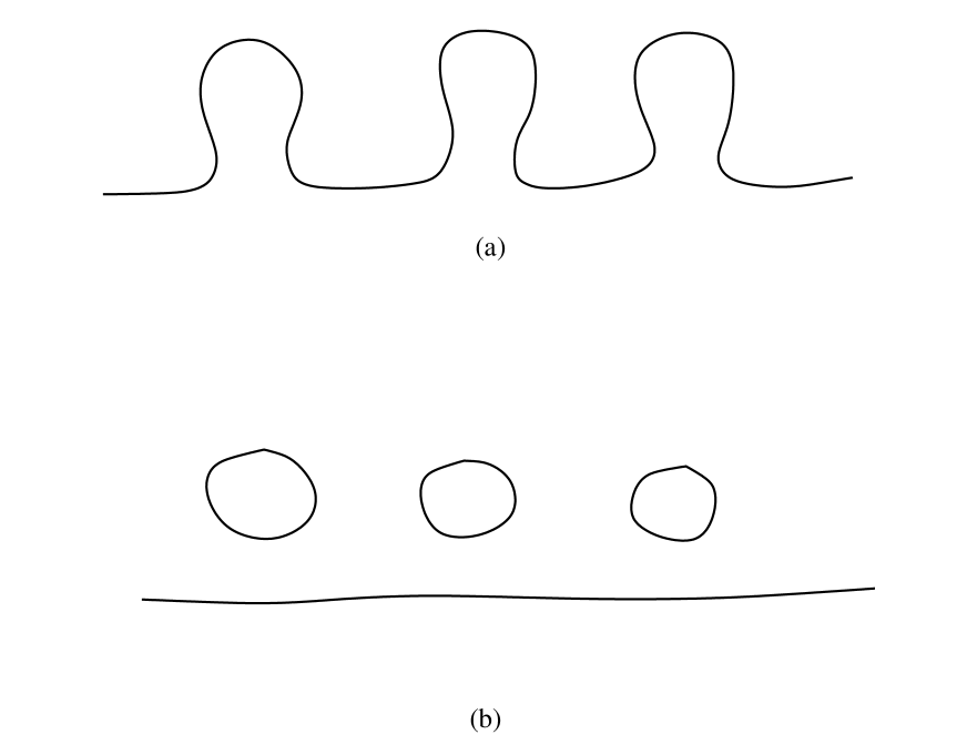
In classical mean-field dynamo theory, turbulence is presumed to arise from nonmagnetic phenomena. Since backreaction of the field on the turbulence is assumed to be unimportant (at least until equipartition strengths are reached) properties of the turbulence, as expressed through the and tensors, are independent of the magnetic field. A dynamo based on the Parker instability represents a departure from this scenario in that the magnetic field (specifically, buoyancy of magnetic flux tubes) drives the -effect. But while the underlying physics of Parker’s model is quite different from that of the classical dynamo, the effective equations are essentially the same. The generation of poloidal field from toroidal field as well as the elimination of ‘unwanted’ flux can be described by and -like terms in an equation for the large-scale field. Moreover the timescale for these processes is similar to what is obtained in the standard scenario.
Moss, Shukurov & Sokoloff (1999) considered a mean-field disk dynamo in which the -effect is driven by the Parker instability. In particular, they incorporated two modifications into the standard dynamo equation (Eq. (74)). First, is taken to be an increasing function of where is the equipartition field strength. Thus, the -effect becomes stronger as the field reaches equipartition, i.e., as the buoyancy of the flux tubes increases. Second, the rotational velocity is supplemented by a term corresponding to motions away from the disk, again due to buoyancy, i.e., also depends on . Solutions obtained from the full three-dimensional dynamo equations were found to resemble those obtained in conventional models in which the -effect comes from cyclonic turbulence. Some important differences did emerge. In particular, it was found that with a buoyancy-driven -effect, the azimuthal field was no longer confined to a thin region near the equatorial plane but rather extended into the halo region.
A variant of the Parker’s model was considered in a series of papers by Hanasz & Lesch (1993, 1997, 1998). In particular, they studied the dynamics of a individual flux tubes under the influence of gravity, pressure from the ambient medium, and buoyancy due to both the magnetic field and cosmic rays pointing out that cosmic ray pressure inside a flux tube will make it buoyant even if the magnetic field is weak. In fact, with a weak field, magnetic tension, which tends to limit the Parker instability, will be unimportant. The hypothesis is then that star formation in an early phase of a galaxy leads to an excess of cosmic ray pressure over magnetic pressure. It is the enhanced buoyancy of the flux tubes due to the cosmic rays that drives and Parker-type fast dynamo, thereby converting cosmic ray energy to magnetic field energy.
IV.8.2 Magnetorotational Instability
Magnetic fields may play a more direct role in the onset of turbulence. Balbus & Hawley (1991) have shown that a powerful, local, shear instability occurs in weakly magnetized differentially rotating disks. Almost any small seed field, in combination with an angular velocity profile that decreases with radius, will lead to dynamical instability. While the instability has been known for some time (Chandrasekhar 1960) it was Balbus & Hawley (1991) who recognized its importance for astrophysical disks (see Balbus & Hawley 1998 for a review).
To understand the origin of the instability, consider an axisymmetric rotating disk with angular velocity and magnetic field parallel to the spin axis. Focus on two fluid elements along the same field line and consider what happens when they are displaced, one in the direction of rotation and the other in the opposite direction. Magnetic tension causes the leading element to slow and move inward and the trailing element to speed up and move outward. If there is differential rotation with the fluid element that flows inward will enter a more rapidly rotating region of the disk and its angular velocity increases stretching the field line is stretched even further. This positive feedback loop is the essence of the instability (Balbus & Hawley 1991).
The instability can act as one component of a magnetohydrodynamic dynamo (e.g., Brandenburg et al. 1995; Hawley, Gammie, & Balbus 1996). The flows due to the instability regenerate magnetic fields which in turn reinforce the turbulence. A surprising feature of this system is that the magnetic energy is somewhat higher than the kinetic energy of the gas, i.e., super-equipartition field strengths are achieved.
It is not clear whether the Balbus-Hawley instability is relevant to galactic magnetic fields. The underlying cause of the instability comes from the tendency of a weak magnetic field to enforce corotation. Since the inner regions of a spiral galaxy are typically in approximate solid body rotation a necessary ingredient for the instability is all but absent. However, the Balbus-Hawley instability may be important in the creation of the magnetic fields that seed the dynamo. It is possible, for example, that seed fields are generated in active galactic nuclei (AGN) and then dispersed through the ISM by jets with the Balbus-Hawley instability playing a central role in the generation of these AGN-fields.
IV.8.3 Cross-Helicity Dynamo
The cross-helicity dynamo is a variant of the standard mean-field dynamo which allows for more rapid amplification of a seed field at early times. The effect was first proposed in a general context by Yoshizawa (1990) and later applied to the problem of galactic magnetic fields by Yokoi (1996) and Brandenburg & Urpin (1998). The model assumes that a cross-correlation exists between the fluctuating components of the velocity and magnetic field, i.e., . The mean-field MHD equation is then supplemented by a term that is proportional to the product of and the large-scale vorticity field, . Since this term is not proportional to the large-scale magnetic field, it leads to linear rather than exponential growth of . Under certain assumptions, the cross-helicity dynamo can dominate at early times speeding up the amplification process (Brandenburg and Urpin 1998).
It is interesting to compare the cross-helicity effect with the standard mechanism. In the cross-helicity dynamo, the mean vorticity distorts through the inertial term in the Euler equation (Eq. (15))
| (105) |
and distorts through the stretching term in the MHD equation (Eq. (8))
| (106) |
| (107) |
If the fluctuation fields are isotropic, . The cross-helicity effect therefore leads to an electromotive force of the form where and is the characteristic correlation or turnover time of the turbulence. When this term is included, the mean-field dynamo equation takes the form
| (108) |
Thus, there is a source term in the induction equation which is independent of the large-scale magnetic field. The effective current associated with this source is parallel to the mean vorticity which, in a disk galaxy, is parallel to the spin axis. Only toroidal fields are generated. By contrast, the -effect generates a current which is parallel to the magnetic field and hence poloidal fields are generated from toroidal ones.
Brandenburg & Urpin (1998) considered the cross-helicity dynamo in the context of galactic magnetic fields. In order to approximate the importance of the effect, they analyzed different data sets from MHD turbulence simulations and concluded that the relative cross-correlation parameter, is in the range . Using values characteristic of spiral galaxies can be parametrized as follows:
| (110) | |||||
The cross-helicity dynamo dominates over the standard -dynamo for values of the field strength where, as before, is the growth rate of the fastest growing dynamo mode. For example, if , the transition from cross-helicity to -dynamo occurs at a field strength (depending on the value used for ) and at a time ). The cross-helicity effect is potentially important in cases where the initial seed field is extremely weak. In the standard dynamo model, a seed field of strength is amplified to a strength of in . In a cross-helicity/-hybrid dynamo, the same field strength can be reached in (Brandenburg & Urpin 1998).
IV.9 Dynamos in Irregular and Elliptical Galaxies and Galaxy Clusters
The existence of microgauss fields in elliptical galaxies and galaxy clusters presents distinct challenges to models for the origin of cosmic magnetic fields. Rotation plays a central role in the mean-field dynamo models devised to explain magnetic fields in disk galaxies, stars, and planets. Rotation provides a resevoir of energy for field amplification through both and effects. In particular, the -effect requires net helicity, or equivalently, mirror symmetry violation in the turbulence. In rapidly rotating systems mirror symmetry violation occurs because of the Coriolis effect. This effect is weak, if not absent, in slow rotating systems such as ellipticals and clusters.
A turbulent dynamo may well operate in ellipticals and clusters, though without rapid rotation the coherence length of the fields is limited by the characteristic scale of the turbulence. In this section, we discuss the necessity of dynamo action in ellipticals and clusters, sources of energy for the generation of turbulence, and the interplay between cooling flows and magnetic fields.
IV.9.1 Elliptical Galaxies
Moss & Shukurov (1996) identified two potential sources for seed fields in elliptical galaxies: stellar magnetic fields ejected into the ISM by supernavae and stellar winds and magnetic remnants that arise if ellipticals formed from mergers of spiral galaxies. The former can lead to fields of about (see below) while the latter can lead to fields or about . In either case, Moss & Shukurov (1996) concluded that the observed microgauss fields in ellipticals require further amplification. Moreover, simple stretching of fields lines by plasma motions without dynamo action is probably unrealistic since Ohmic dissipation will lead to loss of field energy. They therefore concluded that magnetic fields are amplified by dynamo processes. However, the conditions in elliptical galaxies do not appear to support a mean-field dynamo for the reasons discussed above. (See, however, Lesch & Bender (1990) where it is argued that a mean-field dynamo can operate in elliptical galaxies.) Instead, Moss & Shukurov (1996) proposed that fields in ellipticals are amplified by a so-called fluctuation dynamo (Kazantsev, Ruzmaikin, & Sokoloff 1985) in which turbulent motions lead to rapid growth of the rms magnetic field.
Moss & Shukurov (1996) identified on two potential sources of turbulence in ellipticals, ejecta from supernovae and stellar winds and the stirring of the interstellar gas by the random motions of stars. The former gives rise to acoustic turbulence — essentially the random superposition of sound waves — with a characteristic scale . The latter can drive vortical turbulence with a much smaller characteristic scale (). Moss & Shukurov (1996) suggested that amplification of magnetic fields in ellipticals takes place in two stages. First, vortical turbulence, acting as a dynamo, amplifies a seed field to equipartition strengths on scales within a very short ( timescale. Acoustic turbulence amplifies the field and also leads to an increase in the coherence length. The model predicts that the fields in the inner regions of ellipticals will have strengths that range from near the center to at and have a characteristic scale of .
The effects of cooling flows as well as a time-dependent supernovae rate were considered by Mathews & Brighenti (1997). Moreover, they found that compression of the magnetic field in cooling flows could lead to an additional amplification by a factor of . Moreover, the exact value of the field in ellipticals is sensitive to interstellar turbulence in the distant past.
IV.9.2 Clusters
The origin of magnetic fields in clusters is, at present, uncertain. Cluster galaxies are an obvious source of magnetic fields. Material originally associated with individual galaxies is spread throughout the intracluster medium by tidal stripping and galactic outflows. Magnetic fields, tied to the fluid, are likewise dispersed throughout the cluster, albeit with a smaller field strength due to the usual dilution factor. The observation that fields in clusters are comparable in strength to those in galaxies implies that field amplification is occurring in the intracluster medium.
Early attempts to understand the amplification of magnetic fields in clusters focused on dynamo action in galactic wakes (Jaffe 1980; Roland 1981; Ruzmaikin, Sokoloff, & Shukurov 1989). As galaxies move through the intracluster medium they generate a turbulent wake which can presumably support a dynamo. However, more detailed calculations have shown that it is very difficult to produce fields above by this mechanism (Goldman & Rephaeli (1991) and De Young (1992)).
A more promising scenario relies on mergers to drive cluster-scale dynamos (Tribble 1993). Clusters are relatively young systems and most have undergone at least one merger event during the last Hubble time. The amount of energy released during a major merger is comparable to the gravitational and thermal energies of the system and larger than the magnetic energy by a factor . Therefore only a small fraction of the available energy is required to explain cluster fields. Mergers lead naturally to turbulence and shocks in the intracluster medium. The former is necessary for a dynamo while the latter can accelerate particles which can then produce the synchrotron emission. The lifetime of magnetic fields in the intracluster medium can be relatively long (Soker & Sarazin 1990; Tribble 1993). This timescale is set by the rate of magnetic reconnection, which in turn is limited by the Alfvén speed. For a field and electron number density one finds an Alfvén speed so that the reconnection time for magnetic structures is . (Note, however that the timescale for the field to decay is shorter if the field is concentrated in thin flux tubes (Subramanian 1998; Ruzmaikin et al. 1989).) By contrast, the lifetime of synchrotron emitting electrons is short. Relativistic electrons lose energy by inverse Compton scattering off CMB photons. The lifetime at the present epoch is and decreases rapidly with redshift (Tribble 1993). Thus, radio halos fade quickly while cluster magnetic fields survive for periods comparable to the Hubble time. This simple conclusion may explain the rarity of radio halos and the ubiquity of cluster magnetic fields (Tribble 1993).
As in elliptical galaxies, cooling flows can have a significant effect on the magnetic fields in clusters. Magnetic fields in cooling flows are amplified by radial infall and shear (Soker & Sarazin 1990) and can be expected to reach equipartition with the gas. A direct observable effect of these fields is likely to be very strong Faraday rotation that increases rapidly toward the cluster center.
V Seed Fields
Though magnetic fields could have been a feature of the initial conditions of the Universe a more appealing hypothesis is that they are created by physical processes operating after the Big Bang. These first fields can be extremely small since subsequent dynamo action can amplify them by many orders of magnitude. However, even small fields require an explanation (Zel’dovich & Novikov 1983; Rees 1987; Kronberg 1994; Beck et al. 1996; Kulsrud 1999).
The list of proposals for the origin of seed fields is now long and diverse. However no single compelling model has emerged and thus the following questions remain:
-
•
When did magnetic fields first appear? Were they present during big bang nucleosynthesis? recombination? galaxy formation?
-
•
What was the spectrum (strength vs. coherence length) of the first magnetic fields? Was the galactic dynamo seeded by subgalactic, galactic, or supergalactic-scale fields? In the language of the old debate on cosmological structure formation, are galactic magnetic fields a top-down or bottom-up phenomena?
-
•
Is there a connection between the creation of the first fields and the formation of large-scale structure?
-
•
Evidently, a dynamo is necessary to maintian galactic magnetic fields. Is dynamo action also necessary for amplification of an initially small seed field?
Scenarios for seed fields fall into two broad categories, those that rely on ordinary astrophysical processes and those that rely on new and exotic physics. By and large, astrophysical mechanisms exploit the difference in mobility between electrons and ions. This difference can lead to electric currents and hence magnetic fields. Mechanisms of this type can operate during galaxy formation or alternatively they can operate in other systems such as stars and active galactic nuclei. In the latter case, the question is to explain how magnetic fields in those systems make their way into the interstellar or protogalactic medium.
Exotic processes in the very early Universe can also create magnetic fields. There is strong circumstantial evidence that the Universe has undergone a series of phase transitions since the Big Bang including an episode of inflation and the electroweak and quark-hadron transitions. Magnetic fields of interesting strength can arise during these events though their connection to galactic and extragalactic magnetic fields remains unclear.
V.1 Minimum Seed Field for the Galactic Dynamo
What is the minimum seed field required to explain the observed galactic and extragalactic magnetic fields? Uncertainties in our understanding of the dynamo, galaxy formation, and cosmological parameters make this quantity difficult to pin down. In general, the dynamo amplification factor can be written
| (111) |
where is the growth rate for the dominant mode of the dynamo, is the field strength at the time when the dynamo begins to operate, and is the time when the fields reach the observed value .
Irrespective of dynamo action, a seed field that is created prior to galaxy formation is amplified as the protogalactic gas collapses to form a disk. This point was stressed by Lesch & Chiba (1995) who estimated the amount of pre-dynamo amplification that occurs during galaxy formation. Their analysis was based on a simple and well-worn model for the formation of a disk galaxy proposed by Fall & Efstathiou (1980) (see, also White & Rees 1978). According to Fall & Efstathiou (1980), the first stage of galaxy formation is the development of an extended virialized halo of gas and dark matter where the gas and dark matter are assumed to have the same specific angular momentum. Gas elements cool and lose energy but, by assumption, conserve angular momentum. The end result is a disk which, for simple and reasonable choices of initial conditions (e.g., a gas-dark matter halo in solid-body rotation), resembles the disks of present-day galaxies.
In the hierarchical clustering scenario, halos form around peaks in the primordial fluctuation distribution. Small-scale objects collapse first and coalesce to form systems of increasing size. In general, the inner regions of halos form first. The spherical infall model (Gunn & Gott 1972) provides a useful, albeit highly idealized, picture of halo formation. In this model, the mass distribution around a given peak is assumed to be spherically symmetric with a density profile that decreases monotonically with distance from the peak center. The evolution of a protohalo can therefore be described in terms of the dynamics of spherical shells. Initially, the shells expand with the Hubble flow, though eventually they reach a maximum radius known as the turnaround radius , break away from the general expansion and collapse. After a shell collapses, it virializes with the other shells (though this process is not particularly well understood). The model captures certain features of the hierarchical clustering scenario (e.g., inside-out halo formation) while ignoring the complexities of true hierarchical structure formation. A number of results obtained from this model (e.g., characteristic density, halo formation time) are in good agreement with those obtained from N-body simulations of hierarchical structure formations. Simple arguments suggest that the characteristic radius of a virialized shell is roughly one half of the turnaround radius, . For a typical spiral galaxy, . A seed magnetic field created prior to halo formation is therefore amplified by a factor .
A crucial assumption for what follows is that the gas-dark matter halo acquire angular momentum as it forms. In a hierarchical clustering scenario, protogalaxies gain angular momentum through tidal interactions with neighboring protogalaxies (Hoyle 1949; Peebles 1969; White 1984). (Tidal torque theory, of course, requires a departure from spherical symmetry since tidal fields do not couple to spherical shells.) It is common practice to characterize the angular momentum of a system in terms of the dimensionless spin parameter where is the total angular momentum of the system and is its total energy. Roughly speaking, is the square root of the ratio of the centripetal acceleration to the gravitational acceleration. Theoretical analysis and numerical simulations suggest that, for a typical halo, (Peebles 1969; Barnes & Efstathiou 1987).
As described above the second stage in the formation of a disk galaxy, the gas dissipates energy and sinks to the center of the halo’s gravitational potential well where it forms a rotationally supported disk (i.e., a system in which ). If the protogalaxy were composed entirely of gas, the radius of the disk would be . Not only is this value too small (the typical scale radius of a spiral galaxy is ) but the time required for such a the disk to form is greater than the age of the Universe (Peebles 1993). In a CDM model, 90% of a protogalaxy is in the form of collisionless dark matter which remains in an extended halo. In this case, the disk radius is .
Magnetic fields, frozen into the gas, are amplified by a factor . Additional amplification occurs due to the collapse along the spin axis as the gas forms a thin disk. The net pre-dynamo amplification factor is therefore
| (112) |
where is the disk scale height (Lesch & Chiba 1995).
The quantity is model-dependent and not very well known. In Section IV.E, we found
| (113) |
where depending on the functional form of . Dimensional arguments suggest that where is the size of the largest eddies and is the scale height of the disk (Ruzmaikin, Shukurov, and Sokoloff 1988a). With , , and , we find and . Ferrière (1992, 1993) derives the somewhat smaller value for the supernovae-driven model of turbulence and detailed models of a galactic dynamo based on these results give (Ferrière and Schmidt 2000). However, as discussed above, their calculation may underestimate the strength of the -effect from supernovae.
Observations of CMB angular anisotropy, high-redshift supernovae, and large-scale structure indicate that the Universe is spatially flat with and . This conclusion implies an older Universe as compared with one in which . The lower bound on the required seed field is therefore relaxed since there is more time for the dynamo to operate. In a spatially flat, Robertson-Walker Universe,
| (114) | |||||
where, as before, is the scale factor at time with and . An upper bound on is given by the redshift at which a protogalaxy separates from the Hubble flow, collapses, and virializes. Simple estimates based on the spherical infall model suggest a value . However, disks are almost certainly assembled at a much later epoch. Observerations such as the Hubble Space Telescope Deep Field Survey, for example, indicate that disk galaxies at are highly irregular and still in the process of being formed (see, for example, Lowenthal et al. 1997)
A plot of vs. for , , and various choices of is given in Figure 12(a). The amplification factor , assuming a growth rate , is shown on the right-hand vertical axis. Note that scales linearly with . Evidently, varies by several orders of magnitude depending on and . For and , the maximum amplification factor is and therefore a present-day microgauss requires a seed field with strength . (We have not included the amplification which can occur during galaxy formation.)
 |
 |
 |
Davis, Lilley, & Törnquist (1999) argued that the lower bound on the strength of the seed field is or less depending on the cosmological model. Their estimate assumes a lower value for the Hubble constant (), values for the dynamo growth rate as high , and an earlier choice for . The latter value is taken to be the time when a region that corresponds in size to the largest turbulent eddy () breaks away from the Hubble flow and collapses. The implicit assumption is that dynamo processes begin to operate on subgalactic scales well before the disk forms. While this assumption is reasonable, it requires further study. In particular, the estimates for , derived for a disk dynamo, do not necessarily apply to subgalactic objects in an evolving hierarchy of structure.
Observations of microgauss fields in galaxies at moderate redshifts tighten severely the lower bound on seed fields. The results of Kronberg, Perry, and Zukowski (1992) imply while those of Wolfe, Lanzetta, and Oren (1992) suggest a more stringent albeit controversial choice . is also implied by the observations of radio galaxies by Athreya et al. (1998). Figures 12(b) and 12(c) show for and respectively. With , , and , the limit on is tightened to . More severe is the case where the time available for the dynamo to operate is shortened to a few billion years or less and a seed field with is required.
V.2 Astrophysical Mechanisms
The difference in mobility between electrons and ions in an ionized plasma leads to charge separation effects and a breakdown of the MHD approximation. Consider a multicomponent fluid composed of electrons, protons, and photons. (The discussion can be extended easily to include heavier ions and neutral atoms). The momentum equations for the electrons and protons can be written:
| (115) |
| (116) |
where , , , , and are the partial pressure, mass, mass density, number density, and velocity of the electrons and protons (e.g., Spitzer 1962; Sturrock 1994). The rate of momentum transfer from protons to electrons is where is the characteristic timescale of electron-proton collisions. The current density is and therefore, if approximate local charge neutrality holds (i.e., ), .
Also important for some scenarios is the coupling of electrons and photons due to Thomson scattering. In the strong coupling limit, photons behave like an ideal fluid. Thomson scattering leads to an additional momentum transfer term in Eq. (115) of the form where is the Thomson cross section and , , and are respectively the energy density, pressure, and (fluid) velocity of the photon fluid. The momentum equation for the photon fluid is given by
| (117) |
(see, for example, Peebles 1980).
V.2.1 Seed Fields from Radiation-Era Vorticity
An early attempt to explain the origin of seed fields is due to Harrison (1970, 1973) who considered the evolution of a rotating protogalaxy prior to decoupling. During this epoch, electrons and photons are tightly coupled so that, for most purposes, they can be treated as a single fluid. The coupling between electrons and protons is somewhat weaker allowing currents and hence magnetic fields to develop.
Harrison considered a homogeneous, spherical protogalaxy in solid body rotation with radius . As the protogalaxy expands, and remain constant. In the limit that the electron-proton coupling is ignored the angular momenta of the electron-photon and proton fluids are separately conserved, i.e., and are constant. This implies that and . The ions “spin down” faster than the electrons and photons and a current and hence a magnetic field develop.
A more formal derivation of this result, including the electron-proton coupling, follows from Eqs. (115)–(117). The velocity field for Harrison’s spherical protogalaxy can be decomposed into a homogeneous expansion and a circulation flow, i.e., where is the vorticity of the proton fluid. Combining the curl of Eq. (116) with Maxwell’s equations gives
| (118) |
where, because of the assumed homogeneity, the pressure gradient term in Eq. (116) is dropped. In the highly conducting protogalactic medium, the diffusion term is negligible thus yielding the conservation law
| (119) |
where is some initial time characterized by zero magnetic field.
The dynamics of the electrons is determined primarily by the photons. The inertial and gravitational terms in Eq.(115) are therefore neglected leaving what is essentially a constraint equation for the electron velocity field:
| (120) |
The curl of this equation, together with Maxwell’s equations, gives
| (121) |
while the curl of Eq. (117) gives
| (122) |
| (123) |
In deriving this equation we have used the fact that and . In addition, to leading order, we set and , i.e., differences between the electron, proton, and photon velocities enter the calculation only through the collision terms. The desired result, , follows immediately if we take . By way of example, we note that the solar-neighborhood value yields a seed magnetic field .
Harrison’s scenario for the origin of magnetic fields has a number of attractive features which are echoed in subsequent proposals. First, seed fields are generated as part of the galaxy formation process and therefore naturally have a coherence length comparable to the size of the galaxy. Second, the seed fields have a strength that is set by the vorticity of the protogalaxy which can be related to the present-day vorticity in galactic disks, an observable quantity. These fields, though weak, are sufficient to explain present-day galactic fields, provided an efficient dynamo develops to amplify them. The most severe criticism of the model is that, prior to structure formation, vorticity decays rapidly due to the expansion of the Universe (Rees 1987). The implication is that vorticity in disk galaxies in not primordial but rather generated during structure formation. Harrison’s scenario does suggest that there may be a connection between the origin of galactic vorticity and the origin of seed fields.
V.2.2 Biermann Battery Effect
In the hierarchical clustering scenario, protogalaxies acquire rotational angular momentum from the tidal torques produced by their neighbors (Hoyle 1949; Peebles 1969; White 1984). However, gravitational forces alone cannot generate vorticity and therefore its existence in galactic disks must be due to gasdynamical processes such as those that occur in oblique shocks. In an ionized plasma, these same processes produce magnetic fields (Pudritz & Silk 1989; Kulsrud, Cen, Ostriker, & Ryu 1997; Davies & Widrow 2000).
We consider vorticity generation first because it is conceptually simpler. In the absence of electromagnetic effects and viscosity, the evolution of a collisional fluid is given by Eq. (15) with and . Taking the curl yields the following equation for the vorticity:
| (124) |
The source term on the right-hand side comes from gasdynamical effects, namely pressure and density gradients that are not collinear. (The gravitational force term does not appear since the curl of is identically zero.) Vorticity generation is illustrated in Figure 13 where we consider an ideal single component fluid consisting of a particles of mass . The gravitational force is only partially compensated by the pressure gradient force . The acceleration rate for high density regions is greater than the rate from low density regions and therefore the velocity field downstream of the pressure gradient has a nonzero vorticity and shear ().

In an ionized plasma, similar inertial effects lead to electric currents and magnetic fields. This mechanism, known as the Biermann battery effect (Biermann 1950; Roxburgh 1966) can be derived by combining the generalized Ohm’s law with Maxwell’s equations. The former, found by taking the difference of Eqs. (115) and (116) can be written
| (125) | |||||
where terms of order , as well as terms quadratic in the velocities, have been neglected (Spitzer 1962; Sturrock 1994). In addition, we have assumed that local charge neutrality () holds and that the electron and proton partial pressures are equal. The term describes the backreaction of the magnetic field on the fluid. Since, in the present discussion, we are interested in the creation of (small) seed fields, this term can be ignored. In ideal MHD, the left-hand side, which described charge separation effects, is zero. In addition, the pressure gradient term is ignored. We therefore recover the simple form of Ohm’s law: where is essentially the fluid velocity. In the present discussion, we focus on charge separation effects and assume that the conductivity is high and that and are small. The result is a form of Ohm’s law which is relevant to the Biermann effect:
| (126) |
The curl of this equation,
| (127) |
together with Maxwell’s equations, gives
| (128) |
The Biermann effect can be illustrated by the following simple example. (For a similar pedagogical discussion of the Biermann effect in stars, see see Kemp (1982)). Consider, first, the plane-symmetric flow in Figure 14(a). Since the gravitational force on the protons is much greater than that on the electrons, electrostatic equilibrium () requires an electric field where is the effective gravitational force in the rest frame of the fluid. An electrostatic force of this type exists in stars (Rosseland 1924) but is extremely small and inconsequential to understanding stellar structure.
 |
 |
Electrostatic equilibrium is no longer possible when gradients in theremodynamic quantities such as the density and temperature are not parallel to the pressure gradient. This situation is illustrated in Figure 14(b) where the density increases in the -direction. The second term in Eq. (127) is a nonzero vector in the -direction and therefore at least one of the other terms in this equation is nonzero. In fact, since a nonzero implies a time-dependent magnetic field, which in turn implies time-dependent currents, both terms are nonzero. However, the term on the left-hand side is negligible:
| (129) | |||||
where is the typical length scale for the system. We therefore find a time-dependent magnetic field, in agreement with Eq. (128). For the situation shown in Figure 14(b), the magnetic field is in the -direction.
Approximate local charge neutrality implies that where is the ionization fraction. In addition, since the electrons and protons are expected to be in approximate thermal equilibrium, where is the total gas pressure. The source term on the right-hand side of Eq. (128) can therefore be written
| (130) |
and is evidently proportional to the source term for the vorticity.
It is interesting to note that the Biermann effect has been observed in lasar-generated plasmas (Stamper & Ripin 1975; also see Loeb & Eliezer 1986). The schematic diagram of a typical experiment is shown in Figure 15. The plasma has strong temperature and density gradients that are nearly perpendicular leading to a source term for the magnetic field. These magnetic fields, typically megaguass in strength, were studied through Faraday rotation induced on a second laser beam that was shined through the plasma.
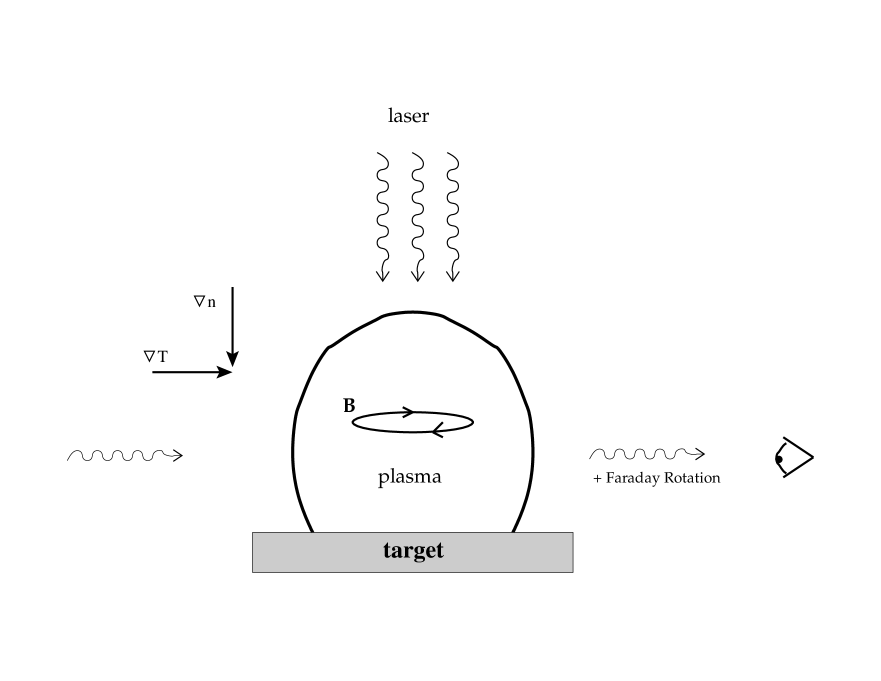
Kulsrud et al. (1997) simulated the creation of magnetic fields via the Biermann battery effect. They used a cosmological hydrodynamic code that was designed to handle shocks as well as gravitational collapse (Ryu et al. 1993). Since the fields are extremely weak, their backreaction on the fluid could be ignored. The MHD equation, supplemented by the Biermann term (Eq. (128)) was solved with obtained from the hydrodynamic code. Kulsrud et al. (1997) assumed parameters appropriate to the CDM model that was popular at the time of their work ( and ) and found that galactic-scale fields are created with strengths of order . However, the spatial resolution of their simulations is , comparable to, if not somewhat larger than, the scales of interest.
Davies & Widrow (2000) took a complementary approach by focusing on the collapse of an isolated galaxy-sized object in an otherwise homogeneous and isotropic universe. Their investigation is in the spirit of semianalytic models of disk galaxy formation by Mestel (1963), Fall & Efstathiou (1980), and Dalcanton, Spergel, & Summers (1997) as well as numerical simulations by Katz & Gunn (1991). However, those models assume that angular momentum and vorticity are present ab initio and therefore they are unable to shed light on voriticity and hence magnetic field generation. In Davies & Widrow (2000) vorticity generation is followed explicitly. The system considered consists of collisionless dark matter and collisional gas with an initial perturbation whose density distribution is assumed to be nearly spherical, smooth (i.e., no small-scale perturbations) and monotonic, specifically, that of an axisymmetric, nonrotating prolate protogalaxy. As discussed above, each fluid element expands to a maximum or turnaround radius before falling in toward the center of the protogalaxy. During the early stages of collapse, an outward moving shock develops and as the infalling gas crosses the shock, it is heated rapidly and decelerated (Bertschinger 1985). In addition, the velocity changes direction at the shock. This is where both magnetic fields and vorticity are generated.
Analytic calculations based on the thin-shock approximation (Landau & Lifshitz 1987) and numerical simulations using SPH follow explicitly the generation of vorticity at the shock that forms. In this simple model, the vorticity and hence magnetic field are in the azimuthal direction and are antisymmetric about the equatorial plane so that the total vorticity of the system is zero. This of course reflects that fact that angular momentum has not been included. Rotation about a short axis of the protogalaxy will “shear” the vorticity and magnetic field lines into a dipole-like configuration.
The results of this analysis indicate that by a redshift , a field, coherent on scales, is generated. This field is amplified by a factor as the protogalaxy collapses (Lesch & Chiba 1995) leading to a field in the fully formed disk galaxy.
In a hierarchical scenario, the Biermann effect also operates in subgalactic objects suggesting an alternate route to galactic-scale seed fields. Consider a region that contains a mass in baryons. This mass corresponds to the Jeans mass at decoupling and represents a lower bound on the mass of the first generation of gravitationally bound objects. Moreover, gas clouds of this size are thought to be the first sites of star-formation. The Biermann effect leads to seed fields of order by (Pudritz & Silk 1989; Davies & Widrow 2000). The dynamical time for these objects is relatively short () and therefore amplification by a dynamo can be very fast. The field reach equipartion (microgauss) strength on these subgalactic scales. As discussed below, small-scales fields of this type can act as a seed for a galactic-scale dynamo. Moreover, the existence of magnetic fields in star-forming clouds may resolve the angular momentum problem for the first generation of stars (Pudritz & Silk 1987).
Lazarian (1992) considered a variant of the Biermann battery in which electron diffusion plays the key role in establishing electric currents and hence magnetic fields. This effect relies on the observation that the ISM is nonuniform, multiphase, and clumpy. Diffusion of electrons from high to low density regions results in an electric field whose curl is given by
| (131) |
Lazarian (1992) estimated that magnetic fields as high as can be generated on large scales in the ISM.
A battery of this type may have operated prior to the epoch of galaxy formation (Subramanian, Narasimha, & Chitre 1994). At decoupling (), protons and electrons combine to form neutral hydrogen. However, the absence of Ly absorption in quasar spectra (above and beyond the features in the Ly forest) severely limit the amount of smoothly distributed HI in the intergalactic medium. The implication is that hydrogen has been reionized almost completely at some epoch between decoupling and (Gunn & Peterson 1965). Subramanian, Narasimha, & Chitre (1994) assumed that reionization is characterized by ionization fronts propagating through the intergalactic medium. Electric currents and magnetic fields are produced when these fronts encounter density inhomogeneities. Gnedin, Ferrara, & Zweibel (2000) performed numerical simulations detailing this mechanism. These simulations followed the reionization of the Universe by stars in protogalaxies. Ionization fronts formed in high density protogalaxies propagate through the Universe. As they cross filamentary structures in the so-called cosmic web, they drive currents which in turn give rise to magnetic fields. The fields produced are highly ordered on a megaparsec scale and have a strength of . Furthermore, the fields are stronger inside dense protogalaxies though a detailed analysis on these scales was limited by resolution of the simulations.
V.2.3 Galactic Magnetic Fields from Stars
The first generation of stars can be a source of galactic-scale seed fields. Even if a star is born without a magnetic field, a Biermann battery will generate a weak field which can be amplified rapidly by a stellar dynamo. If the star explodes or undergoes significant mass loss, magnetized material will be spread throughout the ISM. The following simple argument illustrates why this proposal is attractive (Syrovatskii 1970). Over the lifetime of the Galaxy, there have been supernova events, roughly one for each volume element. The magnetic field in the Crab nebula, taken as the prototypical supernova remnant, is over a region in size. A galaxy filled with (ancient) Crab-like nebulae would therefore have an average field with strength . Similarly, gas lost from stars via a wind will carry stellar magnetic fields into the ISM (Michel & Yahil 1973).
The magnetic fields produced by stars will have a tangled component which is orders of magnitude larger than the coherent component. By contrast, the random and regular components of a typical spiral galaxy are nearly equal. Therefore, stellar magnetic fields, in and of themselves, cannot explain magnetic fields in disk galaxies. Nevertheless, the (rms) large-scale component due to an ensemble of small-scale stellar fields can act as a seed for a galactic dynamo.
A naive model for the large-scale structure of stellar-produced magnetic fields divides the galactic disk into a large number of random cells of size . The magnetic field is assumed to be uniform within each cell but uncorrelated from one cell to the next. The rms flux through a surface of scale is where is the number of cells that intersect the surface. The rms field on the scale is therefore
| (132) |
where is the average field in an individual cell.
A more careful treatment takes into account the expected topology of the magnetic field. In particular, magnetic field lines within an individual cell should close. This point was stressed by Hogan (1983) in his discussion of the magnetic fields produced in a cosmological phase transitions (see, also Ruzmaikin, Sokoloff & Shukurov 1988a, 1988b). Consider an idealized model in which the field within a given cell has a dipole structure. The orientation and strength of the dipoles are assumed to be uncorrelated from one cell to the next. Let us estimate the magnetic flux through a surface enclosed by a circular contour of radius as shown in Figure 16. The contribution to the flux from cells “inside” the contour is identically zero: the only nonzero contribution comes from cells along . The number of such cells is and therefore the flux through scales as . Hence the magnetic field, averaged over a length scale is
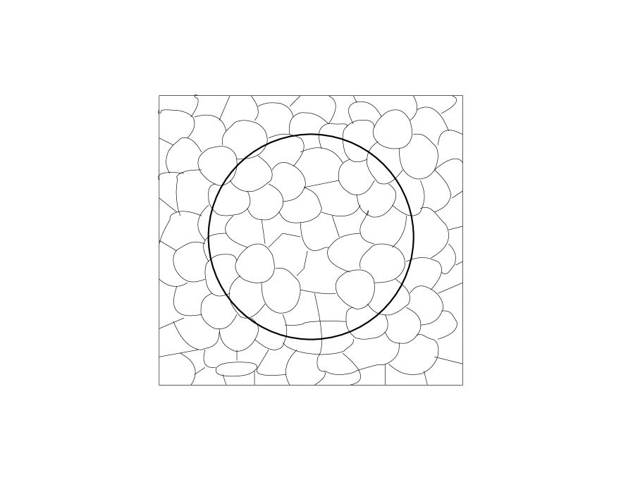
| (133) | |||||
Thus, a significant large-scale magnetic field results if the Galaxy is filled with Crab-like regions.
The proposal that the galactic dynamo is seeded by magnetic fields first created in stars has a potentially fatal flaw: Stars form in protostellar gas clouds. Since the presence of angular momentum in a cloud halts its collapse, efficient angular momentum transport is necessary if star formation is to occur. Magnetic field can remove angular momentum from protostellar clouds, but if the first fields form in stars, then the first clouds will not have any fields. Nevertheless, stellar field may be important in establishing the galactic dynamo. Bisnovatyi-Kogan, Ruzmaikin, & Sunyaev (1973) (see, also Pudritz & Silk 1989) proposed a model in which fields are generated in protostellar clouds by a Biermann-type mechanism and dynamo action. These fields facilitate star formation and the stars that form then act as sites for rapid field amplification. Finally, supernova explosions and stellar winds disperse stellar fields into the ISM thereby seeding the dynamo.
A common thread between the battery mechanism described in the previous section and fields produced by stars is that small-scale fields can provide the seed for a large-scale dynamo. Indeed, the fluctuation dynamo is very efficient at amplifying fields on scales up to that of the largest turbulent eddies () to equipartition strengths on a relatively short timescale. The projection of this highly tangled field onto the dominant mode of an dynamo can act as the seed. The amplitude of this component is, in general, a factor of smaller than the rms field thus giving a seed field of . Simulations of an dynamo seeded by tangled field were carried out by Poedz et al. (1993) and Beck, Poedz, Shukurov & Sokoloff (1994). The initial field was chosen to be random on sub-kiloparsec scales with an rms strength of . At first, the amplitude of the field declines sharply while its scale length increases rapidly. There follows a period of exponential growth to a present day value for the regular field strength of .
V.2.4 Active Galactic Nuclei
Active galactic nuclei (AGN) are promising sites for the production of galactic and extragalactic magnetic fields (Hoyle 1969, Rees 1987, Daly & Loeb 1990; Chakrabarti, Rosner, & Vainshtein 1994, Rees 1994). AGN are powered by the release of gravitational potential energy as material accretes onto a central compact object, presumably a supermassive black hole. There, dynamo processes can amplify magnetic fields on relatively short timescales. Moreover, even if the central region of an AGN forms without a magnetic field, one will develop quickly through Biermann battery-type mechanisms. Finally, well-collimated jets can transport magnetic field energy away from the central object and into the protogalactic or intergalactic medium.
The following order of magnitude estimate, due to Hoyle (1969) gives an indication of the field strengths possible in an AGN scenario. The rotational energy of a compact object and the material in its immediate vicinity (total mass ) can be parametrized as where . Equipartition between the magnetic field and the rotational energy in the fluid (achieved by differential rotation and/or dynamo action) implies a magnetic field strength
| (134) |
where is the volume of the central region. If this field expands adiabatically to fill the volume of the Galaxy, a field with strength
| (135) | |||||
will result. As an example, Hoyle (1969) considers the values , , , and where one finds .
Our understanding of AGN has improved to the extent that detailed discussions of these objects as potential sources of seed magnetic fields is now possible. Daly & Loeb (1990) proposed that the magnetic field in a particular galaxy originates during an AGN phase of that galaxy. This scenario presumes that all galaxies (or at least, all galaxies with strong magnetic fields) have compact central objects, a conjecture that is now supported by numerous observations (see, for example, Magorrian et al. 1998). An AGN phase is characterized by two oppositely-directed, well-collimated jets which transport material into the ISM. Since magnetic fields in the central region are frozen into the jet material, they too are carried into the ISM.
Daly & Loeb (1990) described, in detail, the interaction of the jet with the ISM (also see Daly 1990). A shock forms where this material collides with the ambient gas. At the same time, a blast wave develops propagating perpendicular to the jet axis and carrying magnetized material into the so-called shock cocoon. The timescale for this process is short relative to the lifetime of the galaxy and material from the central AGN engine can reach the outer part of a protogalaxy in a time where is the shock speed and is the length of the jet. An order of magnitude estimate for the strength of the galactic field that results is obtained by assuming that the total magnetic field energy in the jet resides ultimately in the disk galaxy that develops, i.e., where and are the volume and field strength for the jet and and are the corresponding quantities for the disk. If the jet has a mean cross-sectional area and scale length we have
| (136) |
where and are the characteristic height and radius of the disk. Typically, , and . With these values, Daly & Loeb (1990) estimated that the galactic scale would have a strength .
An essential feature of Daly and Loeb’s model is that each galaxy produces its own seed field. An alternative is that a population of AGN at high redshift ‘contaminates’ the protogalactic medium with magnetic field prior to the epoch when most galaxies form (Rees 1987, 1994; Furlanetto & Loeb 2001). The jets that originate in AGN often end in giant radio lobes which are tens of kiloparsecs in size and have magnetic fields . The field in a typical protogalaxy due to pre-galactic AGN is
| (137) |
where is the number density of AGN. Thus, a relatively small number of AGN can seed the protogalactic medium with fields in excess of those produced by battery-type mechanisms.
The amplification of magnetic fields in an accretion-disk environment has been the subject of a number of studies. Pudritz (1981), for example, demonstrated that a mean-field dynamo can operate in a turbulent accretion disk. The Balbus-Hawley instability provides an alternate route to strong fields since a weak magnetic field leads to turbulence which in turn can rapidly amplify the field (Brandenburg et al. 1995; Hawley, Gammie, & Balbus 1996).
Kronberg, Lesch, & Hopp (1999), Birk, Wiechen, Lesch, & Kronberg (2000) considered a somewhat different scenario in which the seed fields for spiral galaxies such as the Milky Way are created in dwarf galaxies that form at a redshift . In their model starburst-driven superwinds rather than jets transport magnetic flux into the IGM. In the hierarchical clustering scenario, dwarf galaxies are the first to form and hence the first to support active star formation. In addition, the consensus is that these systems suffer substantial mass loss via supernovae and stellar winds. The scenario requires that strong magnetic fields exist at early times in dwarf galaxies a reasonable assumption given that star-formation and outflow activity increase the amplification rate in models such as Parker’s (1992) modified -dynamo.
V.3 Seed Fields from Early Universe Physics
The very first magnetic fields may have been created during an early universe phase transition. These events typically involve fundamental changes in the nature of particles and fields as well as a significant release of free energy over a relatively short period of time, two conditions that lead naturally to electric currents and hence magnetic fields. Often, the question is not whether magnetic fields are created during an early universe phase transition, but whether these fields are appropriate seeds for galactic dynamos.
Causality imposes a fundamental constraint on early universe scenarios for the generation of seed fields. The Hubble distance, , sets an upper bound on the size of a region that can be influenced by coherent physical processes. (In a radiation or matter dominated Universe, is, up to a constant of order unity, equal to the causal horizon, i.e., the age of the Universe times the speed of light. Even if an inflationary epoch changes the causal structure of the Universe, still sets an upper limit on the scale over which physical processes can operate.) In comoving coordinates, the Hubble distance reaches the scale of galactic disks at a time after the Big Bang. Contrast this with the age of the Universe at the electroweak phase transition () or QCD phase transition () and the nature of the causality problem becomes clear: Fields generated in the early Universe have a coherence length that is much smaller than what is required of seed fields for a galactic dynamo.
Many of the scenarios that operate after inflation rely on either statistical fluctuations of strong small-scale fields to yield (weak) large-scale ones or dynamical processes, such as an inverse cascade of magnetic energy, to channel field energy from small to large scales. Conversely, scenarios that operate during inflation produce fields on scales up to the present-day Hubble radius. However, these models have their own set of difficulties.
V.3.1 Post-inflation Scenarios
We begin our discussion with the cosmological QCD phase transition (e.g., Boyanovsky 2001). At high temperatures, quarks and gluons are weakly coupled and exist as nearly free particles in a plasma. The transition to the hadronic phase, in which quarks are bound into mesons and baryons, occurs at a temperature . The order of the quark-hadron phase transition is not known. If it is second order, the transformation from quark-gluon plasma to hadrons occurs adiabatically, i.e., approximate thermodynamic equilibrium is maintained locally and at each instant in time. A more dramatic sequence of events occurs if the phase transition is first order. As the Universe cools below , bubbles of hadronic phase nucleate and grow. Shocks develop at the bubble walls, latent heat is released, and the Universe reheats back to . The two phases now coexist with the hadronic regions growing at the expense of regions still in the quark phase.
Hogan (1983) was the first to investigate the possibility that magnetic fields could be generated in a cosmological first-order phase transition. His model assumes that battery and dynamo processes create and amplify magnetic fields, that are concentrated in the bubble walls. When the walls collide the fields from each bubble are “stitched” together by magnetic reconnection. In this way, magnetic field lines, following random paths, can extend to scales much larger than the characteristic scale, , of the bubbles at the time of the phase transition. The situation is analogous to the one that arises with seed fields from stellar outflows and supernovae. The component of the magnetic field that is coherent on scales has a typical strength .
Detailed calculations of magnetic field generation during the electroweak and QCD phase transitions, under the assumption that they are first-order, have been carried out by numerous groups. Quashnock, Loeb, & Spergel (1989), for example, demonstrated that a Biermann battery operates during the QCD phase transition. The baryon asymmetry of the Universe implies that there are more quarks than anti-quarks. If the number densities of the light quarks up, down and strange (charges and respectively) were equal, the quark-gluon plasma would be electrically neutral. However, the strange quark is heavier than the other two and therefore less abundant so that there is a net positive charge for the quarks. This charge is compensated by an excess of negative charge in the lepton sector. Shocks that develop during the nucleation of hadronic bubbles are characterized by strong pressure gradients which affect the quarks and leptons differently. Therefore, electric currents develop as bubble walls sweep through the quark-gluon plasma. Quashnock, Loeb, & Spergel (1989) estimated the strength of the electric fields to be where characterizes the magnitude of the pressure gradient and is the fractional difference between energy densities of the quark and lepton fluids. depends on the details of the transition. A reasonable estimate is which is an order of magnitude or two smaller than the Hubble distance at the time of the phase transition. With , Quashnock, Loeb, & Spergel found . sets the scale for the coherence length of the field. A distance at corresponds to a present present-day distance . The field strength at recombination on these scales is . Assuming (Hogan 1983) this yields a galactic-scale () field with strength at recombination of .
At the time of the QCD phase transition, the energy density of the Universe is corresponding to an equipartition field strength of . Thus, the battery mechanism proposed by Quashnock, Loeb, & Spergel (1989) taps into a tiny fraction of the available energy. Cheng & Olinto (1994) and Sigl, Olinto, & Jedamzik (1997) suggested that stronger field-generating mechanisms operate during the coexistence phase that follows bubble nucleation. As hadronic regions grow, there is a tendency for baryons to concentrate in the quark phase. Essentially, the bubble walls act as ‘snowplows’ sweeping up baryons. In doing so, they create currents of order where is the number density of positive charge carriers in the quark phase and is the typical velocity of the bubble walls. The corresponding magnetic field is where is the thickness of the charge layer. For reasonable parameters, this leads to an estimate on scales of at . If , a field strength at recombination on scales (comoving coordinates) will be .
A first-order electroweak phase transition can also generate large-scale magnetic fields (Baym, Bödeker, & McLerran 1996; Sigl, Olinto, & Jedamzik 1997). During the electroweak phase transition, the gauge symmetry breaks from the electroweak group to the electromagnetism group . The transition appears to be weakly first order or second order depending on parameters such as the mass of the Higgs particle (Boyanovsky 2001; Baym, Bödeker, & McLerran 1996 and references therein). If it is first order, the plasma supercools below the electroweak temperature . Bubbles of broken symmetry phase nucleate and expand, eventually filling the Universe. As in the case of the QCD transition, we write the bubble size where and . The wall velocities are believed to be in the range . Baym, Bödeker, & McLerran 1996 discussed the structure of the bubble walls and the associated shocks in detail. The key observation is that the fluid becomes turbulent where two walls collide. Fully developed MHD turbulence leads rapidly to equipartition of field energy up to the scale of the largest eddies in the fluid, assumed to be comparable to . Thus, the field strength on this scale is
| (138) | |||||
where is the energy density at the time of the electroweak phase transition.
Magnetic fields can arise in cosmological phase transitions even if they are second order (Vachaspati 1991). In the standard model, electroweak symmetry breaking occurs when the Higgs field acquires a vacuum expectation value (VEV): . Interactions between and the gauge fields are described by the kinetic energy term in the Lagrangian which can be written where is the covariant derivative and is the coupling constant. (Gauge group indices have been suppressed.) In principle, and can conspire to give . However, since all quantities are uncorrelated over distances greater than the Hubble distance at the time of the phase transition, , in general, does not vanish (Vachaspati 1991). Dimensional arguments imply where is the correlation length for the field at the time of the phase transition. The correlation length is actually set by the temperature and is much smaller than the Hubble length: . We are interested in the electromagnetic field which is but one component of the complete set of gauge fields . Vachaspati (1991) finds which, using dimensional analysis, implies a field strength .
To estimate the field strength on larger scales Vachaspati (1991) assumed that executes a random walk on the vacuum manifold with stepsize . Over a distance where is a large number, the field will change, on average, by . Thus, the gradient in the Higgs field is . The magnetic field strength, at the time of the phase transition, will be . On a galactic scale ( in comoving coordinates; ) at decoupling, we find .
A somewhat different analysis by Enqvist & Olesen (1993) suggests that the magnetic fields decrease with scale more slowly than suggested by Vachaspati (1991). They argued that the mean magnetic field satisfies
| (139) |
where denotes an average over regions of size . Thus, in their model, .
Dynamical mechanisms can also lead to an increase in the coherence length of a magnetic field that is produced in an early Universe phase transition. Cornwall (1997), Son (1999) and Field & Carroll (2000) have considered the transfer of magnetic field energy from small to large scales by a process known as inverse cascade. This process occurs when there is substantial magnetic helicity in a fluid (Pouquet, Frisch, & Lèorat 1976). Assume that small-scale helicity is injected into the fluid in a short period of time. Magnetic energy will shift from small to large scales as the system attempts to equilibrate while conserving magnetic helicity and total energy. An inverse cascade in a cosmological context leads to the following scaling laws for the field energy and coherence length:
| (140) |
and
| (141) |
where is the time when the fields are created. In the above analysis, it is assumed that the inverse cascade operates during the radiation-dominated but not matter-dominated phase of the Universe. For illustrative purposes, Field & Carroll (2000) considered the evolution of fields created at the electroweak scale. The coherence scale and strength of these initial fields are written as and where and are dimensionless parameters. Today, these fields would have a coherence length and scale and . Thus, if the generation mechanism is efficient in producing horizon-sized helical fields then the result will be strong fields on very large scales. However, no compelling mechanism is known for generating large net helicity in a cosmic fluid and therefore scenarios based on the inverse cascade must be considered highly speculative.
V.3.2 Inflation-Produced Magnetic Fields
The inflationary Universe paradigm provides both the kinematic and dynamical means of producing a nearly scale-free spectrum of energy density perturbations (e.g., Kolb & Turner 1990 and references therein). This feature makes inflation an attractive candidate for the production of magnetic fields (Turner & Widrow 1988).
In most models, inflation is driven by the dynamics of a weakly coupled scalar field known as the inflaton. During inflation, the energy density of the Universe is dominated by the vacuum energy of the inflaton (Guth 1981; Linde 1982; Albrecht & Steinhardt 1982). Since this energy density is approximately constant, the Universe is in a nearly de Sitter phase with and . Exponential growth of the scale factor has two important consequences. First, during inflation the physical length corresponding to a fixed comoving scale grows relative to the (nearly constant) Hubble distance . By contrast, during the radiation and matter dominated epochs, grows more slowly than . Therefore, a given mode of fixed comoving size (e.g., a single Fourier component of a small-amplitude density perturbation) starts out subhorizon-sized and crosses outside a Hubble volume during inflation only to reenter the Hubble volume during either radiation or matter dominated epochs (Figure 17). Microphysical processes can influence this mode during the first subhorizon-sized phase. In particular, de Sitter space quantum-mechanical fluctuations continuously excite all massless or very light fields (i.e., all fields whose Compton wavelength is greater than ). Both the amplitude and coherence length of these fluctuations are set by the Hubble parameter so that the energy density per logarithmic wavenumber bin in these excitations at the time when they are produced is . Therefore, to the extent that is constant during inflation (or more generally, a power-law function of time) the fluctuation spectrum is scale-free.

While all massless fields are excited during inflation, their subsequent evolution varies dramatically depending on how they couple to gravity. Fluctuations of the inflaton give rise to an energy-density perturbation spectrum at second horizon crossing that is consistent with what is required to explain large-scale structure in the Universe (Guth & Pi 1982; Starobinskii 1982; Hawking 1982; Bardeen, Steinhardt, & Turner 1983). In simple inflationary Universe models, perturbations have an amplitude at second horizon crossing that is approximately constant with scale. This result is consistent with what is called for in hierarchical clustering models and is in agreement with measurements of the angular power spectrum of microwave background anisotropies.
Quantum-produced de Sitter-space fluctuations in minimally coupled scalar fields (i.e., fields that do not couple explicitly to the Ricci scalar ) and in gravitons can also be significant (see, Kolb & Turner 1990 and references therein). By contrast, since electromagnetic fields are conformally coupled to gravity, the energy density in a fluctuation decreases as leading to amplitudes that are uninterestingly small. Conformal invariance must therefore be broken in order to produce significant primeval magnetic flux.
In a conformally trivial theory, the field equations are invariant under a rescaling of lengths at each location in space. Likewise, conformally flat spacetimes, such as de Sitter space and the radiation and matter dominated Robertson-Walker models, can be written as (time-dependent) rescalings of Minkowski space. It follows that the form of the field equations of a conformally invariant theory in a conformally flat spacetime are time-independent. For example, the equations of motion for the magnetic field in a Robertson-Walker space time are:
| (142) |
where is the conformal time related to the clock time through the expression . For massive fields, conformal invariance is broken by the introduction of a length scale, namely, the Compton wavelength. Conformal invariance can also be broken through couplings to other fields.
Turner & Widrow (1988) suggested a number of ways of breaking conformal invariance in electromagnetism: (1) introduce the gravitational couplings , , , etc; (2) couple the photon to a charged field that is not conformally coupled to gravity; (3) couple the photon to an axion-like field. Only (1) was considered in any great detail. The terms are the least attractive possibility since they explicitly break gauge invariance by giving the photon an effective mass. However, computationally, this case is the easiest to analyze and for a wide range of parameters (the coupling constants for the various terms) interesting large-scale magnetic fields can be generated. The terms are theoretically more palpable but the fields that result are very small.
Numerous authors have attempted to find more natural and effective ways to break conformal invariance. Ratra (1992) calculated the spectrum of magnetic fields produced in a set of inflation models characterized by the inflaton potential . Potentials of this type can be motivated by superstring theory. Ratra (1992) assumed a coupling of the inflaton to electromagnetism through a term and found that fields as large as could be produced.
Magnetic fields due to a charged scalar field were considered by Calzetta, Kandus, & Mazzitelli (1998) and Kandus et al. (2000). These authors found that charged domains form during inflation which give rise to currents and hence magnetic fields during the post-inflation era. A different mechanism has been proposed by Davis et al. (2001) who show that the backreaction of the scalar field gives the gauge field an effective mass thus breaking conformal invariance. The mechanism is attractive, in part, because it operates in the standard model. Actually, it is the standard-model -boson that is amplified through its coupling to the Higgs field. As inflation comes to a close, the fluctuations in the field are transferred to the hypercharge field (i.e., a linear combination of the and photon fields). The boson acquires a mass at the electroweak scale leaving behind pure magnetic field. Davis et al. (2001) obtain a magnetic field strength of order on a scale of provided certain conditions during reheating are met.
Garretson, Field, & Carroll (1992) analyzed the amplification of inflation-produced electromagnetic fluctuations by their coupling to a PGB. This coupling, which takes the form , leads to exponential growth but only for modes whose wavelength is smaller than the Hubble radius. No amplification is found for modes outside the horizon. The net result is that large-scale magnetic fields of an interesting strength are not produced by this mechanism.
VI Summary and Conclusions
It was the late 1940’s when the Galactic magnetic field was independently proposed by theorists and detected by observers. Since then, galactic and extragalactic magnetic fields have been the subject of intense and fruitful research. Nevertheless, fundamental questions concerning their origin, evolution, and nature remain unanswered.
Magnetic fields have been detected in over one hundred spiral galaxies, in numerous elliptical and irregular galaxies, in galaxy clusters, and in the Coma supercluster complex. New instruments such as the planned square kilometer array radio telescope will no doubt reveal new magnetic structures.
It is of interest to note that at present, there is no example of a meaningful null detection of magnetic field in a collapsing or virialized system. Conversely, only upper limits exist on the strength of truly cosmological magnetic fields. The fact that these limits are several orders of magnitude lower than the strength of galactic and cluster fields suggests that magnetic fields are amplified, if not created, during structure formation and evolution.
The magnetic fields found in spiral galaxies are unusual in that the strength of the large-scale component is comparable to that of the tangled component. By contrast, the fields in ellipticals are random on scales. Likewise, cluster fields are tangled on the scale of the cluster itself. The distinction no doubt reflects a key difference between spiral galaxies on the one hand and ellipticals and clusters on the other. Namely, the stellar and gaseous disks of spiral galaxies are dynamically “cold”, rotationally supported systems while ellipticals and clusters are dynamically “hot”. Evidently, the scale of the largest component of the magnetic field in any system is comparable to the scale of the largest coherent bulk flows in that system.
The -dynamo is the most widely accepted paradigm for the amplification and maintenance of magnetic fields in spiral galaxies. The hypothesis that magnetic fields are continuously regenerated by the combined action of differential rotation and helical turbulence is compelling especially in light of the observation that the magnetic structures in disk galaxies are in general spiral. One may think of these structures as the MHD analogue of material spiral arms. Spiral structure is believed to be a wavelike phenomenon where the crests of the waves are characterized by enhanced star-formation activity which, in turn, is triggered by an increase in the local density. Likewise, magnetic spiral arms may reflect low-order eigenmodes in a disklike magnetized system. A more direct connection between material and magnetic spiral structure is evident in certain galaxies where strong magnetic fields appear in the regions between the material arms. The FIR-radio continuum correlation provides further evidence in support of a connection between star formation and large-scale galactic magnetic fields.
The magnetic fields in ellipticals and clusters require a different explanation. Mergers may play the central role in the establishment of these fields since they are likely to be present in merger remnants, typically tidally shredded spiral galaxies. The magnetic debris from merger events can act as seeds for subsequent dynamo action. In addition, the energy released during a merger event can drive turbulence in the interstellar or intercluster medium. It is unlikely that either ellipticals or clusters will support an -dynamo since differential rotation in these systems is relatively weak. However, they may support fluctuation dynamos in which turbulence amplifies magnetic fields on scales up to the size of the largest eddies in the systems.
From a theoretical perspective, the greatest challenge in the study of galactic magnetic fields comes from the tremendous dynamic range involved. The scale radius and height of a typical galactic disk are of order and , respectively, while turbulent eddies in the ISM extend in size from subparsec to scales. Naive arguments suggest that even if initially, magnetic energy is concentrated at large scales, in a turbulent medium, there is a rapid cascade of energy to small scales. A mean-field approximation, where velocity and magnetic fields are decomposed into large-scale and small-scale components, bypasses this problem. The equation for the large-scale magnetic field, known as the dynamo equation, incorporates the effects of the small-scale fields through the and tensors which, in turn, attempt to capture the gross properties of the turbulence (e.g., helicity, spatial anisotropy).
The dynamo equation for an axisymmetric thin disk can be solved by means of a quasi-separation of variables which leads to eigenvalue equations in , , , and . The -eigenvalue gives the growth rate of the magnetic field while the -eigenvalue characterizes the symmetry of the field under rotations about the spin-axis of the disk. The equation is similar, in form, to the Schrödinger equation and its eigenvalue feeds back into into the value of the growth rate. The separation-of-variables analysis has yielded a number of encouraging results. Chief among these is a demonstration of principle, namely, that disklike systems with a rotation curve similar to that of a spiral galaxy, can support a magnetic dynamo. Numerical simulations provide the means to study more realistic models. In particular, the effects of a finite disk thickness and deviations from axisymmetry can be explored. These investigations suggest ways in which bisymmetric and/or odd party magnetic fields can be excited.
Unless one is willing to accept magnetic fields as a property of the Big Bang, their existence today implies a violation of the MHD approximation at some stage during the history of the Universe. While MHD processes can stretch, twist, and amplify magnetic field, by definition, they cannot generate new field where none already exist. Proposals for the origin of the first magnetic fields are as varied as they are imaginative. For example, interest in the exotic environment of the very early Universe, and in particular cosmological phase transitions, has spawned numerous ideas for the creation of seed magnetic fields. A perhaps more appealing set of proposals relies on the ordinary astrophysical phenomena that occur during structure formation. Magnetic fields will develop in AGN, stars, and the shocks that arise during gravitational collapse. Indeed, rough estimates suggest that AGN and/or an early generation of stars will yield fields of strength on galactic scales. Dynamo action can amplify a field of this strength to microgauss levels by a redshift , a result consistent with observations of magnetic fields in high-redshift radio galaxies.
The astrophysical mechanisms mentioned above were proposed at a time when our understanding of structure formation was relatively crude. It is in part for this reason that the creation of seed fields and the dynamo have been treated as separate and distinct processes. Indeed, most studies of disk dynamos do not make specific references to particular models for seed field production. Likewise, few papers on seed fields follow the resultant fields into the dynamo regime.
Today, semi-analytic models and numerical simulations enable us to study galaxy formation in detail, taking into account hierarchical clustering, tidal torques from nearby objects, gasdynamics, and feedback from star formation. Moreover, observations of high-redshift supernovae, the CMB angular anisotropy spectrum, and large scale structure have pinned down key cosmological parameters such as the densities of baryons and dark matter and the Hubble constant. In light of these developments, it may be possible to achieve a more complete description of the origin of galactic magnetic fields, one that begins with the production of seed fields and follows smoothly into the dynamo regime.
Acknowledgements.
I am grateful to J. Irwin, D. McNeil, A. Olinto, and S. Toews for carefully reading and commenting on early versions of the manuscript and to R. Beck and A. Shukurov extremely detailed and valuable suggestions. I am also grateful to P. Kronberg and R. Beck for providing several of the figures. Finally, I would like to thank O. Blaes, G. Davies, R. Henriksen, J. Irwin, P. Kronberg, C. Thompson, and J. Weingartner for useful discussions. This work is supported in part by the Natural Sciences and Engineering Research Council of Canada.References
- (1) Albrecht, A. & Steinhardt, P. J. 1982, Phys. Rev. Lett. , 48, 1220
- (2) Alfvén, H. 1949, Phys. Rev., 75, 1732
- (3) Athreya, R. M., Kapahi, V. K., McCarthy, P. J., & van Breugel, W. 1998, A& A 329, 809
- (4) Asseo, E. & Sol, H. 1985, Physics Reports, 148, 307
- (5) Bahcall, N. A., Ostriker, J. P., Perlmutter, S., & Steinhardt, P. J. 1999, Science, 284, 1481
- (6) Balbi, A. et al. 2000, Astrophys. J. , 545, L1
- (7) Balbus, S. A. & Hawley, J. F. 1991, Astrophys. J. , 376, 214
- (8) Balbus, S. A. & Hawley, J. F. 1998, Rev. Mod. Phys. , 70, 1
- (9) Bardeen, J. M., Steinhardt, P. J., & Turner, M. S. 1983, Phys. Rev. D, 28, 679
- (10) Barnes, J., Efstathiou, G. 1987, Astrophys. J. , 319, 575
- (11) Baryshnikova, Iu., Shukurov, A., Ruzmaikin, A., & Sokoloff, D. D. 1987, A&A, 177, 27
- (12) Barrow, J. D., Ferreira, P. G., & Silk, J. 1997, Phys. Rev. Lett. , 78, 3610
- (13) Baym, G., Bödeker, & McLerran, L. 1996, Phys. Rev. D53, 662
- (14) Beck, R. 1982, A&A, 106, 121
- (15) Beck, R., Poezd, A. D., Shukurov, A., Sokoloff, D. 1994, A&A 289, 94
- (16) Beck, R. Brandenburg, A. Moss, D., Shukurov, A., Sokoloff, D. 1996, AARA, 34, 155
- (17) Beck, R. & Hoernes, P. 1996, Nature, 379, 47
- (18) Beck, R. et al. 1999, Nature, 397, 324
- (19) Beck, R. 2000, Phil. Trans. R. Soc. Lond. A, 358, 777
- (20) Beck, R. 2002, in The Astrophysics of Galactic Cosmic Rays, eds. Diehl, R. et al. (Kluwer, Dordrecht, The Netherlands)
- (21) Belyanin, M. P., Sokoloff, D. D., & Shukurov, A. M. 1994, Russ. J. of Math. Phys., 2, 149
- (22) Berkhuijsen, E. M. et al. 1997, A&A, 318, 700
- (23) Bertschinger, E. 1985, Astrophys. J. S, 58, 39
- (24) Bi, H. & Davidsen, A. F. 1997, Astrophys. J. , 479, 523
- (25) Biermann, L. 1950, Zs. Naturforsch., 5a, 65
- (26) Binney, J. J. & Merrifield, M. 1998 Galactic Astronomy (Princeton, NJ: Princeton University Press)
- (27) Birk, G. T., Wiechen, H., Lesch, H., & Kronberg, P. P. 2000, A&A, 353, 108
- (28) Bisnovatyi-Kogan, G. S., Ruzmaikin, A. A., & Sunyaev, R. A. 1973, Sov. Ast. 17, 137
- (29) Blackman, E. G. & Field, G. B. 1999, Astrophys. J. , 521, 597
- (30) Blackman, E. G. & Field, G. B. 2000, Astrophys. J. , 534, 984
- (31) Blasi, P., Burles, S., & Olinto, A. V. 1997, Astrophys. J. , 514, 79L
- (32) Blasi, P. & Olinto, A. V. 1999, Phys. Rev. D, 59, 023001
- (33) Boyanovsky, D. 2001, in NATA Advanced Study Institute: Phase Transitions in the Early Universe: Theory and Observation, ed. de Vega et al. (Kluwer, Dordrecht/London) p 3.
- (34) Brandenburg, A. & Donner, K. J. 1997, MNRAS, 288, L29
- (35) Brandenburg, A. et al. 1992, A&A, 259, 453
- (36) Brandenburg, A. et al. 1993, A&A, 271, 36
- (37) Brandenburg, A., Nordlund, A., Stein, R. F., & Torkelsson, U. 1995, Astrophys. J. , 446, 741
- (38) Brandenburg, A. & Urpin, V. 1998, A&A, 332, L41
- (39) Brandenburg, A. & Zweibel, E. G. 1994, Astrophys. J. , 427, L91
- (40) Brecher, K. & Blumenthal, G. 1970, Astrophys. Lett., 6, 169
- (41) Burbidge, G. R. 1956, Astrophys. J. , 124, 416
- (42) Calzetta, E. A., Kandus, A., & Mazzitelli, F. D. 1998, Phys. Rev. D57, 7139
- (43) Cattaneo, F. & Vainshtein, S. I. 1991, Astrophys. J. , 376, L21
- (44) Cattaneo, F. & Hughes, D. W. 1996, Phys. Rev. E, 54, 4532
- (45) Cesarsky, C. J. 1980, AARA, 18, 289
- (46) Chakrabarti, S. K., Rosner, R., & Vainshtein, S. I. 1994, Nature, 368, 434
- (47) Chandrasekhar, S. 1960, Proc. Nat. Acad. Sci., 46, 53
- (48) Cheng, B, Schramm, D. N., & Truran, J. W. 1994, Phys. Rev. D, 49, 5006
- (49) Cheng, B, Olinto, A. V., Schramm, D. N., & Truran, J. W. 1996, Phys. Rev. D, 54, 4714
- (50) Cheng, B. & Olinto, A. V. 1994, Phys. Rev. D, 50, 2421
- (51) Chyzy, K. T. et al. 2000, A&A, 355, 128
- (52) Clarke, T. E., Kronberg, P. P. & Boehringer, H. 2001, Astrophys. J. , 547, 111
- (53) Coles, P. & Jones, B. 1991, MNRAS, 248, 1
- (54) Cornwall, J. M. 1997, Phys. Rev. D, 56, 6146
- (55) Dahlem, M. 1997, PASP, 109, 1298
- (56) Dalcanton, J. Spergel, D., & Summers, F. 1997, Astrophys. J. , 482, 659
- (57) Daly, R. A. 1990, Astrophys. J. , 355, 416
- (58) Daly, R. A. & Loeb, A. 1990, Astrophys. J. , 364, 451
- (59) Davies, G. & Widrow, L. M. 2000, Astrophys. J. , 540, 755
- (60) Davis, J. & Greenstein, J. L. 1951, Astrophys. J. , 114, 206
- (61) Davis, A.-C., Lilley, M., & Törnkvist 1999, Phys. Rev. D60 021301
- (62) Davis, A.-C., K. Dimopoulos, T. Prokopec, & O. Tornkvist 2001, Phys. Lett. B, 501, 165
- (63) de Bernardis, P. et al. 2000, Astrophys. J. , 536, L63
- (64) De Young, D. S. 1992, Astrophys. J. , 386, 464
- (65) Dolag, K., Bartelmann, M. & Lesch, H 1999, A&A, 351
- (66) Donner, K. J. & Brandenburg, A. 1990, A&A, 240, 289
- (67) Dumke, M., Krause, M., Wielebinski, R., & Klein, U. 1995, A&A, 302, 691
- (68) Duric, N. 1990, in Galactic and Intergalactic Magnetic Fields, IAU Symp. 140 (eds Beck, R., Kronberg, P. P. & Wielebinski, R.), 235
- (69) Durrer, R., Kahniashvili, T. & Yates, A. 1998, Phys. Rev. D, 58, 123004
- (70) Edge, A. C., Stewart, G. C., & Fabian, A. C. 1992, MNRAS, 258, 177
- (71) Elstner, D., Meinel, R., & Rüdiger 1990, Geophys. Astrophys. Fluid Dynamics, 50, 85
- (72) Elstner, D., Meinel, & Beck, R. 1992, A&AS, 94, 587
- (73) Elstner, D., Otmianowska-Mazur, K., von Linden, S., & Urbanik, M. 2000, A&A 357, 129
- (74) Ensslin et al. 2001, Astrophys. J. , 549, 39L
- (75) Enqvist, K. & Olesen, P. 1993, Phys. Lett. , 319, 198
- (76) Fabian, A. C., Nulsen, P. E., Canizares, C. R. 1984, Nature, 310, 733
- (77) Fabian, A. C. 1994, ARAA, 32, 277
- (78) Fall, S. M. & Efstathiou, G. 1980, MNRAS, 193, 189
- (79) Fan, Z. & Lou, Y.-Q. 1996, Nature, 383, 800
- (80) Fendt, Ch., Beck, R., & Neininger, N. 1998, A&A, 335, 123
- (81) Fermi, E. 1949, Phys. Rev., 75, 1169
- (82) Ferrière, K. 1992, Astrophys. J. , 389, 286
- (83) Ferrière, K. 1993, Astrophys. J. , 404, 162
- (84) Ferrière, K. 1998, A&A, 335, 488
- (85) Ferrière, K. & Schmitt, D. 2000, A&A, 358, 125
- (86) Field, G. B. 1995, in The Physics of the Interstellar Medium and Intergalactic Medium, ASPC Volume 80, ed. Ferrara, A. et al. 1.
- (87) Field, G. B. & Carroll, S. M., 2000, Phys. Rev. D, 62, 103008
- (88) Fitt, A. J. & Alexander, P. 1993, MNRAS, 261, 445
- (89) Fixen, D. J. et al. 1996, Astrophys. J. , 473, 576
- (90) Freidberg, J. P., 1987, Ideal Magnetohydrodynamics (Plenum Press, London)
- (91) Frick, P. et al. 2000, MNRAS, 318, 925
- (92) Frick, P., Stepanov, R., Shukurov, A., & Sokoloff, D. D. 2001, MNRAS, 325, 649
- (93) Furlanetto, S. R. & Loeb, A. 2001, Astrophys. J. , 556, 619
- (94) Gaensler, B. M. et al. 2001, Astrophys. J. , 549, 959
- (95) Garretson, W. D., Field, G. B., & Carroll, S. M. 1992, Phys. Rev. D, 46, 5346
- (96) Ginzburg, V. L. & Syrovatskii, S. I. 1964, The Origin of Cosmic Rays (Pergamon Press, Oxford)
- (97) Goldman, I. & Rephaeli, Y. 1991, Astrophys. J. , 380, 344
- (98) Golla, G. & Hummel, E. 1994, A&A, 284, 777
- (99) Gnedin, N. Y., Ferrara, A., & Zweibel, E. G. 2000, Astrophys. J. , 539, 505
- (100) Grasso, D. & Rubinstein, H. R. 1996, Phys. Letts., B379 73
- (101) Greenfield, P. E., Roberts, D. H., & Burke, B. F. 1985, Astrophys. J. , 293, 370
- (102) Greisen, K. 1966, Phys. Rev. Lett. , 16, 748
- (103) Gruzinov, A. V. & Diamond, P. H. 1994, Phys. Rev. Lett. , 72, 1651
- (104) Gunn, J. E. & Peterson, B. A. 1965, Astrophys. J. , 142, 1633
- (105) Gunn, J. E. & Gott, J. R. 1972, Astrophys. J. , 176, 1
- (106) Guth, A. H. 1981, Phys. Rev. D, 23, 347
- (107) Guth, A. H. & Pi, S.-Y. 1982, Phys. Rev. Lett. , 49, 1110
- (108) Hale, G. E. 1908, Astrophys. J. , 28, 315
- (109) Hall, J. S. 1949, Science, 109, 166
- (110) Han, J. L., Beck, R., & Berkhuijsen, E. M. 1997, A&A, 335, 1117
- (111) Han, J. L., Manchester, R. N., Berkhuijsen, E. M., & Beck, R. 1997, A&A, 322, 98
- (112) Hanisch, R. J. 1982, A&A, 116, 137
- (113) Hanasz, M. & Lesch, H. 1993, A&A, 278, 561
- (114) Hanasz, M. & Lesch, H. 1997, A&A, 321, 1007
- (115) Hanasz, M. & Lesch, H. 1998, A&A, 332, 77
- (116) Harrison, E. R. 1970, MNRAS, 147, 279
- (117) Harrison, E. R. 1973, Phys. Rev. Lett. , 30, 18
- (118) Hawking, S. W. 1982, Phys. Lett. B115, 295
- (119) Hawley, J. F., Gammie, C. F., & Balbus, S. A. 1996, Astrophys. J. , 464, 690
- (120) Heiles, C. 1987, in Interstellar Processes (eds Hollenbach, D. J. & Thronson, H. A.), 171
- (121) Heiles, C. 1990, in Galactic and Extragalactic Magnetic Fields, IAU Symp. 140 (eds Beck, R., Kronberg, P. P. & Wielebinski, R.), 35
- (122) Hillas, A. M. 1998, Nature, 395, 15
- (123) Hiltner, W. A. 1949a, Nature, 163, 283
- (124) Hiltner, W. A. 1949b, Science, 109, 165
- (125) Hogan, C. J. 1983, Phys. Rev. Lett. , 51, 1488
- (126) Howard, A. M. & Kulsrud, R. M. 1997, Astrophys. J. , 483, 648
- (127) Hoyle, F. 1949, in Proc. Symposium on Motion of Gaseous Masses of Cosmical Dimensions, Problems of Cosmical Aerodynamics, ed. J. M. Burgers & H. C. van de Hulst (Dayton: Central Air Documents Office), p. 195
- (128) Hoyle, F. 1958, in La Structure et L’evolution de L’univers: XI Conseil de Physique Solvay, Bruxelles (ed. R. Stoops), 53
- (129) Hoyle, F. 1969, Nature, 223, 936
- (130) Hummel, E., Beck, R., and Dahlem, M. 1991, A&A, 248, 23
- (131) Hummel, E. et al. 1988, A&A, 199, 91
- (132) Jackson, J. D. 1975, Classical Electrodynamics (2nd Edition) (Wiley: New York)
- (133) Jaffe, W. J. 1980, Astrophys. J. 241, 925
- (134) Jedamzik, K., Katalinic, V., & Olinto, A. V. 1998, Phys. Rev. D, 57, 3264
- (135) Jedamzik, K., Katalinic, V., & Olinto, A. V. 2000, Phys. Rev. Lett. , 85, 700
- (136) Kandus, A., Calzetta, E. A., Mazzitelli, F. D., Wagner, C. E. M. 2000, Phys. Lett. B472, 287
- (137) Katz, N. & Gunn, J. E. 1991, Astrophys. J. , 377, 365
- (138) Kazantsev, A. P., Ruzmaikin, A. A., & Sokoloff, D. D. 1985, Zh. Exper. Teor. Fiz., 88, 487 (JETP, 61, 285)
- (139) Kazès, I., Troland, T. H., & Crutcher, R. M. 1991, A&A, 245, L17
- (140) Kemp, J. C. 1982, PASP, 94, 627
- (141) Kernan, P., Starkman, G. D., & Vachaspati, T. 1996, Phys. Rev. D, 54, 7207
- (142) Kernan, P., Starkman, G. D., & Vachaspati, T. 1997, Phys. Rev. D, 56, 3766
- (143) Kim, K.-T., Kronberg, P. P., Giovannini, G., & Venturi, T. 1989, Nature, 341, 720
- (144) Kim, E.-J., Olinto, A. V., & Rosner, R. 1996, Astrophys. J. , 468, 28
- (145) Kim, K.-T., Tribble, P. C., & Kronberg, P. P., 1991, Astrophys. J. , 379, 80
- (146) Kim, K.-T., Kronberg, P. P., Dewdney, P. E., Landecker, T. L., 1990, Astrophys. J. , 355, 29
- (147) Klein, U., Wielebinski, R., & Morsi, H. W. 1988, A&A, 190, 41
- (148) Kolatt, T. 1998, Astrophys. J. , 495, 564
- (149) Kolb, E. W. & Turner, M. S. 1990, The Early Universe (Addison-Wesley, Reading, MA)
- (150) Korpi, M. J. et al. 1999, Astrophys. J. , 514, L99
- (151) Kosowsky, A. & Loeb, A. 1996, Astrophys. J. , 469, 1
- (152) Krasheninnikova, Iu., Shukurov, A., Ruzmaikin, A. A., & Sokoloff, D. D. 1989, A&A, 213, 19
- (153) Krause, F. & Wielebinski, R. 1991, Rev. Mod. Astron., 4, 260
- (154) Krause, F. & Beck, R. 1998, A&A, 335, 789
- (155) Krause, F. & Rädler, K. -H. 1980, “Mean-Field Magnetohydrodynamics and Dynamo Theory” (Pergamon Press: Oxford)
- (156) Krause, M. 1990, in Galactic and Extragalactic Magnetic Fields, IAU Symp. 140 (eds Beck, R., Kronberg, P. P. & Wielebinski, R.), 196
- (157) Krause, M., Hummel, E., & Beck, R. 1989a, A&A, 217, 4
- (158) Krause, M., Hummel, E., & Beck, R. 1989b, A&A, 217, 17
- (159) Kronberg, P. P. 1977, in Radio Astronomy and Cosmology, IAU Symp. 74 (ed. Jauncey, D. L.), 367
- (160) Kronberg, P. P. 1994, Rep. Prog. Phys., 57, 325
- (161) Kronberg, P. P., Lesch, H., & Hopp, U. 1999, Astrophys. J. , 511, 56
- (162) Kronberg, P. P. & Perry, J. P. 1982, Astrophys. J. 263, 518
- (163) Kronberg, P. P., Perry, J. P., & Zukowski, E. L. H. 1992, Astrophys. J. 387, 528
- (164) Kronberg, P. P. & Simard-Normandin, M. 1976, Nature, 263, 653
- (165) Kulsrud, R. M. 1990, in Galactic and Extragalactic Magnetic Fields, IAU Symp. 140 (eds Beck, R., Kronberg, P. P. & Wielebinski, R.), 527
- (166) Kulsrud, R. M. & Anderson, S. W. 1992, Astrophys. J. , 396, 606
- (167) Kulsrud, R. M., Cen, R., Ostriker, J. P. & Ryu, D. 1997, 480, 481
- (168) Kulsrud, R. M. 1999, AARA, 37, 37
- (169) Landau, L. D. & Lifshitz, E. M. 1987, Fluid Mechanics (London: Pergamon Press)
- (170) Larmor, J. 1919, in Rep. 87th Meeting Brit. Assoc. Adv. Sci., Bournemouth, 159
- (171) Lawler, J. M. & Dennison, B., 1982, Astrophys. J. 252, 81
- (172) Lazarian, A. 1992, A&A, 264, 326
- (173) Lazarian, A., Goodman, A. A., & Myers, P. C. 1997, Astrophys. J. , 490, 273
- (174) Leahy, J. P. 1991, in Beams and Jets in Astrophysics (ed. Hughes, P. A.), 100
- (175) Lemoine, M. Sigl. G., Olinto, A. V., Schramm, D. N. 1997, Astrophys. J. , 486, L115
- (176) Lesch, H. & Bender, R. 1990, A&A 233, 417
- (177) Lesch, H. & Chiba, M. 1995, A&A, 297, 305
- (178) Linde, A. D. 1982, Phys. Lett. 108B, 389
- (179) Loeb, A. & Eliezer, S. 1986, Phys. Rev. Lett. , 56, 2252
- (180) Lowenthal, J. D. 1997, Astrophys. J. , 481, 673
- (181) Madsen, M. S. 1989, MNRAS, 237, 109
- (182) Magorrian, J. et al. 1998, AJ, 115, 2285
- (183) Manchester, R. N. 1974, Astrophys. J. , 188, 637
- (184) Mathewson, D. S. & Ford, V. L. 1970, Mem. R. astr. Soc., 74, 139
- (185) Mathews, W. G. & Brighenti, F. 1997, Astrophys. J. , 488, 595
- (186) Mestel, L. 1963, MNRAS, 126, 553
- (187) Mestel, L. & Subramanian, K. 1991, MNRAS, 248, 677
- (188) Mestel, L. & Subramanian, K. 1993, MNRAS, 265, 649
- (189) Michel, F. C. & Yahil, A. 1973, Astrophys. J. , 179, 771
- (190) Milgrom, M. & Usov, V. 1995, Astrophys. J. , 449, L37
- (191) Milne, E. A. 1924, Proc. Cambridge. Phil. Soc., 22, 493
- (192) Moffatt, H. K. 1978, Magnetic Field Generation in Electrically Conducting Fluids, Cambridge Univ. Press, Cambridge
- (193) Monaghan, J. J. 1992, ARAA, 30, 543
- (194) Moss, D. & Shukurov, A. 1996, MNRAS, 279, 229
- (195) Moss, D., Shukurov, A. & Sokoloff, D. D. 1999, A&A, 343, 120
- (196) Moss, D., Shukurov, A., Sokoloff, D. D., Beck, R., & Fletcher, A. 2001, A&A, 380, 55
- (197) Mould, J. R. et al. 2000, Astrophys. J. , 529, 768
- (198) Niklas, S. & Beck, R. 1997, A&A, 320, 54
- (199) Olive, K. A., Steigman, G., & Walker, T. P. 2000, Phys. Rep., 389, 333
- (200) Oren, A. L. & Wolfe, A. M. 1995, Astrophys. J. , 445, 624
- (201) Panesar, J. S. & Nelson, A. H. 1992, 264, 77
- (202) Parker, E. N. 1970, Astrophys. J. 162, 665
- (203) Parker, E. N. 1971, Astrophys. J. 163, 255
- (204) Parker, E. N. 1973a, Astrophys. Space Sci. 22, 279
- (205) Parker, E. N. 1973b, Astrophys. Space Sci. 24, 279
- (206) Parker, E. N. 1979, Cosmical Magnetic Fields (Oxford: Clarendon)
- (207) Parker, E. N. 1992, Astrophys. J. , 401, 137
- (208) Peebles, P. J. E. 1969, Astrophys. J. , 155, 393
- (209) Peebles, P. J. E. 1980, The Large-Scale Structure of the Universe, Princeton University Press, Princeton, NY
- (210) Peebles, P. J. E. 1993, Principles of Physical Cosmology, Princeton University Press, Princeton, NY.
- (211) Perry, J. J., Watson, A. M.& Kronberg, P. P., 1993, Astrophys. J. , 406, 407
- (212) Phillipps, S. et al. 1981, A&A 103, 405
- (213) Piddington, J. H. 1964, MNRAS, 128, 345
- (214) Piddington, J. H. 1972, Cosmic Electrodynamics, 3, 60
- (215) Plaga, R. 1995, Nature, 374, 430
- (216) Poedz, A., Shukurov, D., & Sokoloff, D. 1993, MNRAS, 264, 285
- (217) Pouquet, A., Frisch, U., & Lèorat, 1976, J. Fluid. Mech. 77, 321
- (218) Priklonsky, V., Shukurov, A., Sokoloff, D. D., & Soward, A. 2000, Geophys. Astrophys. Fluid Dynamics, 93, 97
- (219) Pryke, C. et al. 2002, Astrophys. J. , 568, 46
- (220) Pudritz, R. E. 1981, MNRAS, 195, 881
- (221) Pudritz, R. E. & Silk, J. 1989, Astrophys. J. , 342, 650
- (222) Quashnock, J., Loeb, A. & Spergel, D. 1989, Astrophys. J. , 344, L49
- (223) Rafikov, R. R. & Kulsrud, R. 2000, MNRAS, 316, 249
- (224) Rand, R. J. & Lyne, A. G. 1994, A&A, 268, 497
- (225) Ratra, B. 1992, Astrophys. J. , 391, L1
- (226) Rees, M. J. QJRAS, 1987, 28, 197
- (227) Rees, M. J. 1994, in Cosmical Magnetism, ed. D. Lynden-Bell (The Netherlands: Dordrecht), p. 155
- (228) Rees, M. J. & Reinhardt, M. 1972, A&A, 19, 189
- (229) Reid, M. J. & Siverstein, E. M. 1990, Astrophys. J. , 361, 483
- (230) Rephaeli, Y. 1979, Astrophys. J. , 227, 364
- (231) Rephaeli, Y. & Gruber, D. E. 1988, Astrophys. J. , 333, 133
- (232) Reuter, H.-P. et al. 1992, A&A, 256, 10
- (233) Roettighr, K., Stone, J. M., & Burns, J. O. 1999, Astrophys. J. , 518, 594
- (234) Rohde, R. & Elstner, D. 1998, A&A, 333, 27
- (235) Rohde, R., Beck, R. & Elstner, D. 1999, A&A, 350, 423
- (236) Roland, J. 1981, A&A, 93, 407
- (237) Roxburgh, I. W. 1966, MNRAS132, 201
- (238) Rosseland, S. 1924, MNRAS, 84, 720
- (239) Ruzmaikin, A. A., Shukurov, A. M., & Sokoloff, D. D. 1988a, Magnetic Fields in Galaxies (Dordrecht: Kluwer)
- (240) Ruzmaikin, A. A., Shukurov, A. M., & Sokoloff, D. D. 1988b, Nature, 336, 341
- (241) Ruzmaikin, A. A., Shukurov, A. M., & Sokoloff, D. D. 1989, MNRAS, 241, 1
- (242) Ruzmaikin, A. A., Shukurov, A. M., Sokoloff, D. D., & Beck, R. 1990, A&A, 230, 284
- (243) Ryu, D., Ostriker, J. P., Kang, H. & Cen, R. 1993, Astrophys. J. , 4141
- (244) Sarazin, C. L. 1986, in Radio continuum Processes in Clusters of Galaxies, 36
- (245) Sargent, W. L. W., Young, P. J., Boksenberg, A., & Tytler, D. 1980, Astrophys. J. Supp., 42, 41
- (246) Scarrott, S. M., Ward-Thompson, D., & Warren-Smith, R. F. 1987, MNRAS, 224, 299
- (247) Scarrott, S. M., Rolph, C. D., Wolstencroft, R. N., & Tadhunter, C. N. 1991, MNRAS, 249, 16
- (248) Schmidt, M. 1959, Astrophys. J. , 129, 243
- (249) Schramm, D. N. & Turner, M. S. 1998, Rev. Mod. Phys., 70, 303
- (250) Shukurov, A. M. 1998, MNRAS, 299, L21
- (251) Shukurov, A. M. 1999, in Plasma Turbulence and Energetic Particles in Astrophysics, eds. Ostrowski, M. & Schlickeiser, R. (Uniwersytet Jagiellonski, Krakow), p. 66.
- (252) Sigl, G., Olinto, A. V., & Jedamzik, K. 1997, Phys. Rev. D, 55, 4582
- (253) Silk, J. 1968, Astrophys. J. , 151, 459
- (254) Sofue, Y., Fujimoto, M., & Kawabata, K. 1968, Pub. Astr. Soc. Japan, 20, 388
- (255) Sofue, Y., Fujimoto, M., & Wielebinski 1986, ARAA, 24, 459
- (256) Sofue, Y., Takano, T., & Fujimoto, M. 1980, A&A, 91, 335
- (257) Soker, N. & Sarazin, C. L. 1990, Astrophys. J. , 348, 73
- (258) Sokoloff, D. D. & Shukurov, A. M. 1990, Nature, 347, 51
- (259) Sokoloff, D. D., Shukurov, A. M., & Krause, M, 1992, A&A, 264, 396
- (260) Sokoloff, D. D. et al. 1998, MNRAS, 299, 189 (erratum: 1999, MNRAS, 303, 207)
- (261) Son, D. T. 1999, Phys. Rev. D, 59, 063008
- (262) Spitzer, L. 1962, Physics of Fully Ionized Gases, Wiley & Sons, New York
- (263) Spruit, H. C. 1981, A&A, 102, 129
- (264) Stamper, J. A. & Ripin, B. H. 1975, Phys. Rev. Lett. , 34, 138
- (265) Starobinskii, A. A. 1982, Phys. Lett. 117B, 175
- (266) Steenbeck, M., Krause, F. & Rädler, K.-H. 1966, Zs. f. Naturforschung 21, 369
- (267) Stone, J. M. & Norman, M. 1992, Astrophys. J. S., 80, 753
- (268) Stone, J. M. & Norman, M. 1992, Astrophys. J. S., 80, 791
- (269) Sturrock, P. A. 1994, Plasma Physics (Cambridge University Press: Cambridge, UK)
- (270) Subramanian, K. 1998, MNRAS, 294, 718
- (271) Subramanian, K., Narasimha, D., & Chitre, S. M., MNRAS, 271, L15
- (272) Subramanian, K. & Barrow, J. D. 1998, Phys. Rev. Lett. , 81, 3575
- (273) Sukumar, S. & Allen, R. J. 1989, Nature, 340, 537
- (274) Sukumar, S. & Allen, R. J. 1991, Astrophys. J. , 382, 100
- (275) Syrovatskii, S. I. 1970, in Interstellar Gas Dynamics, IAU Symp. 39, 192
- (276) Takeda, M. 1998, Phys. Rev. Lett. , 81, 1163
- (277) Taylor, G. B., Barton, E. J., & Ge, J. 1994, AJ, 107, 1942
- (278) Tosa, M. & Fujimoto, M. 1978, Pub. Astr. Soc. Pac., 30, 315
- (279) Tribble, P. C. 1993, MNRAS, 263, 31
- (280) Trimble, V. 1990 in Galactic and Extragalactic Magnetic Fields, IAU Symp. 140 (eds Beck, R., Kronberg, P. P. & Wielebinski, R.), 29
- (281) Tüllmann, R. et al. 2000, A&A, 364, L36
- (282) Turner, M. S. & Widrow, L. M. 1988, Phys. Rev. D37, 2743
- (283) Urbanik, M., Otmianowska-Mazur, K. & Beck, R. 1994, A&A, 287, 410
- (284) Vachaspati, T. 1991, Phys. Lett. B, 265, 258
- (285) Vainshtein, S. I., Sagdeev, R. Z., Rosner, R., & Kim, E.-J. 1996, Phys. Rev. E, 53, 4729
- (286) Vainshtein, S. I. & Zel’dovich, Ya. B. 1972, Usp. Fiz. Nauk., 106, 431 [Sov. Phys. Usp. 15, 159]
- (287) Vainshtein, S. I. & Cattaneo, F. 1992, Astrophys. J. , 393, 165
- (288) Vainshtein, S. I., Parker, E. N., & Rosner, R. 1993, Astrophys. J. , 404, 773
- (289) Vainshtein, S. I. & Ruzmaiken, A. A. 1971, Astron. J. (SSSR) 48, 902 (Sov. Astron. 15, 714, 1972)
- (290) Vainshtein, S. I. & Ruzmaiken, A. A. 1972, Astron. J. (SSSR) 49, 449 (Sov. Astron. 16, 365, 1972)
- (291) Vallée, J. P. 1975, Nature, 254, 23
- (292) Vallée, J. P. 1990, Astrophys. J. , 360, 1
- (293) Vallée, J. P. 1997, Fund. of Cosmic. Phys., 19, 1
- (294) Verschuur, G. L. 1995, Astrophys. J. , 451, 645
- (295) Vietri, M. 1995, Astrophys. J. , 453, 883
- (296) Wasserman, I. 1978, Astrophys. J. , 224, 337
- (297) Waxman, E. 1995, Phys. Rev. Lett. , 75, 386
- (298) Waxman, E. & Miralda-Escudé, J. 1996, Astrophys. J. , 472, L89
- (299) Welter, G. L., Perry, J. J., & Kronberg, P. P. 1984, Astrophys. J. , 279, 19
- (300) White, S. D. M. & Rees, M. J. 1978, MNRAS, 183, 341
- (301) White, S. D. M. 1984, Astrophys. J. , 286, 38
- (302) Wolfe, A. M., Lanzetta, K. M. & Oren, A. L. 1992, Astrophys. J. , 388, 17
- (303) Yokoi, N. 1996, A&A, 311, 731
- (304) Yoshizawa, A. 1990, Phys. Fluids B, 2, 1589
- (305) Zatsepin, G. T. & Kuzmin, V. A. 1966, JETP Lett. 4, 78
- (306) Zel’dovich, Ya. B. 1957, Sov. Phys. JETP, 4, 460
- (307) Zel’dovich, Ya. B. 1983, Relativistic Astrophysics, Vol. 2: The Structure and Evolution of the Universe, University of Chicago Press, Chicago
- (308) Zel’dovich, Ya. B., Ruzmaikin, A. A., & Sokoloff, D. D. 1983, Magnetic Fields in Astrophysics, Gordon & Breach, New York
- (309) Zel’dovich, Ya. B., Ruzmaikin, A. A., & Sokoloff, D. D. 1990, The Almighty Chance, World Scientific, Singapore
- (310) Zweibel, E. G. 1988, Astrophys. J. , 329, 384
- (311) Zweibel, E. G. & Heiles, C. 1997, Nature, 385, 131