The nature and size of the optical continuum source in QSO 2237+0305

Abstract

From the peak of a gravitational microlensing high-magnification event in the A component of QSO 2237+0305, which was accurately monitored by the GLITP collaboration, we derived new information on the nature and size of the optical $V$-band and $R$-band sources in the far quasar. If the microlensing peak is caused by a microcaustic crossing, we firstly obtained that the standard accretion disk is a scenario more reliable/feasible than other usual axially symmetric models. Moreover, the standard scenario fits both the $V$-band and $R$-band observations with reduced chi-square values very close to one. Taking into account all these results, a standard accretion disk around a supermassive black hole is a good candidate to be the optical continuum main source in QSO 2237+0305. Secondly, using the standard source model and a robust upper limit on the transverse galactic velocity, we inferred that 90 per cent of the $V$-band and $R$-band luminosities are emitted from a region with radial size less than 1.2 10^-2 pc (= 3.7 10¹⁶ cm, at 2$\sigma$ confidence level).

1 Introduction

In the optical continuum, QSO 2237+0305 is a gravitational mirage that consists of four compact components (A-D) round the nucleus of the deflector (lens galaxy). The light bundles corresponding to the components are passing through the bulge of the lens galaxy, and thus, if the galactic mass at the QSO image positions is mainly in stars, the optical depths to microlensing are as high as $\sim 0.5$ (e.g., Schmidt, Webster & Lewis 1998). In this scenario with large normalized surface mass densities, given a component, microlensing violent events will result from the source either crossing a microcaustic, passing close to a microcusp, or traveling through a network of microcaustics (e.g., Schneider, Ehlers & Falco 1992). On the other hand, a microlensing violent episode in the light curve of a component can be easily distinguished from a intrinsic variation, since the intrinsic variability must be observed in all four components of the system with extremely short time delays (e.g., Wambsganss & Paczyński 1994; Chae, Turnshek & Khersonsky 1998; Schmidt, Webster & Lewis 1998). However, when the four brightness records of the QSO images have different non-flat shapes, a direct separation between the true microlensing fluctuations and the possible intrinsic variation cannot be achieved. In the case of four incoherent and non-flat observational trends, to find the true microlensing behaviours we must do some hypothesis on the intrinsic variability.

Irwin et al. (1989) discovered microlensing variability in the quadruple system QSO 2237+0305, and that first evidence was confirmed by other observers (Corrigan et al. 1991; Østensen et al. 1996; Woźniak et al. 2000a,b; Schmidt et al. 2001; Alcalde et al. 2002). In very recent years, two gravitational microlensing high-magnification events (HMEs) were clearly detected by the OGLE collaboration (Woźniak et al. 2000b) and corroborated by the GLITP monitoring (Alcalde et al. 2002). As each individual HME is directly related to the intrinsic surface brightness of the source, the two HMEs in the $V$ band reported by the OGLE team were used to obtain two measurements of both the optical continuum ($V$-band) source size and the rate of brightness decline (Shalyapin 2001). Shalyapin (2001) compared the observational data included in each HME with the time evolution expected from an axially symmetric source crossing a single straight fold caustic. To describe the brightness distribution of the $V$-band source, he used a power-law model: $I_{V}(r)=2^{p_{V}}I_{V}(1+r^{2}/R_{V}^{2})^{-p_{V}}$, which is determined by a typical radius $R_{V}$, a typical intensity $I_{V}=I_{V}(R_{V})$, and a power-law index $p_{V}$. The expected microlensing light curves depend on five free parameters, and the most relevant ones are $\Delta t=R_{V}/V_{\perp}$ and $p_{V}$. We note that a direct measurement of the typical radius $R_{V}$ is not possible, however, using some upper limit on the quasar velocity perpendicular to the caustic line ($V_{\perp}$), it can be obtained a very interesting constraint on the source size as measured by means of the typical radius of the 2D brightness distribution. A crossing time of $\Delta t\approx$ 90 days is inferred from the HME observed in the light curve of the component A, whereas a shorter crossing time of about 30 days is consistent with the HME corresponding to the image C. However, the whole HME of image A (from day 1200 to day 1800) seems to be caused by a complex magnification, which is different to the single straight fold caustic magnification law. In other words, when the main portion of the source is far away from the fold caustic of interest (before day 1400 and after day 1600), there is evidence for a rare behaviour, and so, the fit to the whole microlensing event in the brightness record of the component A could give biased estimates of the parameters. Taking into account this perspective, we only take the results based on the HME corresponding to the image C as non-biased parameter estimates. The value of $\Delta t\approx$ 30 days together with the velocity constraint by Wyithe, Webster & Turner (1999) give an upper limit on the $V$-band typical radius of $R_{V}\leq$ 3 10^-4 pc. A similar conclusion was obtained by Yonehara (2001), who analyzed the same microlensing event but using a different picture and a typical microlens mass of $\approx$ 0.1 $M_{\odot}$ (Wyithe, Webster & Turner 2000). On the other hand, Shalyapin (2001) found that the value of the power-law index is close to the validity limit of the model ($p_{V}\sim$ 1) and the best-fit reduced $\chi^{2}$ is significantly greater than 1.

Apart from the very recent papers by Shalyapin (2001) and Yonehara (2001), other previous works also discussed the size of the optical continuum source (e.g., Wambsganss, Paczynski & Schneider 1990; Webster et al. 1991; Wyithe et al. 2000). These first studies are based on a poorly sampled HME which was observed in Q2237+0305A during late 1988. While the continuum mostly arises from a compact source, the line emission comes from a much larger region. From two-dimensional spectroscopy of QSO 2237+0305, Mediavilla et al. (1998) found an arc of extended C III]$\lambda$1909 emission that connects the components A, D, and B. The observed arc is consistent with a source radius larger than 100 pc.

The GLITP (Gravitational Lenses International Time Project) collaboration has monitored QSO 2237+0305 in the period ranging from 1999 October to 2000 February (Alcalde et al. 2002). The GLITP/PSFphotII photometry in the $V$ and $R$ bands (see Fig. 1 in Alcalde et al. 2002), showed a peak in the flux of the component A and a relatively important gradient in the flux of the component C. These features are related to the two HMEs that were discovered by the OGLE team. The GLITP light curve for image A traced the peak of the corresponding HME, i.e., the maximum and its surroundings, with an unprecedented quality. For example, the OGLE collaboration sampled the $V$-band peak at 19 dates, whereas the GLITP record included measurements of the $V$-flux at 52 dates. Moreover, the rest of global behaviours (components B-D) were accurately drawn from the GLITP photometry (in this paper, we will use the PSFphotII variant). The $VR$ light curves of the four components A-D have been also analyzed from a phenomenological point of view, and the global flat shape for the light curve of Q2237+0305D suggested that the microlensing signal in D and the intrinsic signal are both globally stationary. In consequence of this result, it seems that the global variabilities in A-C are unambiguously caused by microlensing.

As mentioned here above, the whole HME of Q2237+0305A seems to be originated by a complex magnification law. However, in principle, the peak of the HME (just when the main portion of the source crossed a microcaustic) could be a structure mainly caused by a single straight fold caustic, i.e., the curvature and other possible close microcaustics do not significantly perturb the simple magnification law. We adopt this last point of view, and take the GLITP light curve for image A, including only data points very close to the maximum of the HME, to be fitted to the microlensing curves resulting from sources crossing a single straight fold caustic. We remark that the high asymmetry of the peak as well as probabilistic arguments are two strong reasons against an interpretation of the microlensing peak based on a source passing close to a single cusp caustic.

In Section 2 we present the expected microlensing light curves when axially symmetric sources cross a single straight fold caustic, and the fitting procedure. We use a set of axisymmetric sources: brightness distributions enhanced at the centre of the source (standard physical profile, Gaussian profile, and $p$ = 3/2, 5/2 power-law profiles) and the uniform brightness distribution (e.g., Shakura & Sunyaev 1973; Schneider & Weiss 1987; Shalyapin 2001). Section 3 is devoted to the parameter estimation from the comparison between the GLITP microlensing peak in the component A and the expected time evolutions for the different source models. A discussion on the V-band and R-band source sizes, the source size ratio ($R_{V}/R_{R}$), and the reliability of the source models is also included in Section 3. In this paper, to obtain information on the dimension of the $V$-band and $R$-band sources, we will use the measurements of the transverse galactic velocity reported by Wyithe, Webster & Turner (1999). Finally, in Section 4 we summarize our results and conclusions.

2 Theoretical microlensing light curves and fitting procedure

When a source crosses a single straight fold caustic, a microlensing violent phenomenon occurs. This is seen as an important fluctuation in the flux of an image of the source. We are going to describe the properties of a family of axisymmetric sources, present the time evolution of the flux (microlensing curve) corresponding to each source model, and finally, introduce the methodology to compare the theoretical curves with observational data.

2.1 Source models

2.1.1 Uniform and Gaussian disks

In a given optical band ($U$, $B$, $V$, $R$, $I$, …), the two simplest surface brightness distributions are a uniform disk and a Gaussian disk (e.g., Schneider & Weiss 1987). For the source of uniform intensity, one has a well-defined source radius $R_{opt}(source)$ that coincides with the typical radius of the intensity distribution $R_{opt}$. Both radii contain the total brightness of the source. However, for the source with Gaussian intensity distribution and other sources with distributions enhanced at the central regions, we know a typical radius of the 2D profile ($R_{opt}$), and assume that $R_{opt}(source)\gg R_{opt}$. This last hypothesis permits us to justify the approximation $\int_{0}^{R_{opt}(source)}\approx\int_{0}^{\infty}$. For example, in the Gaussian case with $I_{opt}(r)=eI_{opt}\exp(-r^{2}/R_{opt}^{2})$, the total brightness included in the circle with radius $R_{opt}(source)$ is given by $I_{opt}(source)=I_{\infty}\{1-\exp[-R_{opt}^{2}(source)/R_{opt}^{2}]\}$, where $I_{\infty}$ is the brightness derived from an integration between $r$ = 0 and $r$ = $\infty$. If $R_{opt}(source)\gg R_{opt}$, we have $I_{opt}(source)\approx I_{\infty}$. We note that $I_{opt}=I_{opt}(R_{opt})$ is the intensity at the typical radius $R_{opt}$ (i.e., a typical intensity), and so, $I_{opt}(0)=eI_{opt}$ for the Gaussian law. As different models have typical radii with different meanings, in a unified scheme, we define two source sizes: the source radius containing half of the total brightness, $R_{opt}(50\%)$, and the source radius containing 90% of the total brightness, $R_{opt}(90\%)$. Using factors $k(50\%)$ and $k(90\%)$, which depend on the source model, the radii $R_{opt}(50\%)$ and $R_{opt}(90\%)$ can be expressed in terms of the typical radius $R_{opt}$ [e.g., $R_{opt}(50\%)=k(50\%)R_{opt}$]. For a uniform disk, the factors are $k(50\%)=1/\sqrt{2}$ and $k(90\%)=3/\sqrt{10}$, while for a Gaussian disk, we obtain $k(50\%)=\sqrt{\ln 2}$ and $k(90\%)=\sqrt{\ln 10}$.

2.1.2 Power-law models

A more interesting set of source models is the family of intensity profiles with behaviours ($p_{opt}>$ 1)

$$I_{opt}(r)=2^{p_{opt}}I_{opt}(1+r^{2}/R_{opt}^{2})^{-p_{opt}}.$$ (1)

Along with the simplicity of the trends, these power-law models allow to calculate the expected microlensing curves in an analytical way (see Shalyapin 2001, and the next subsection 2.2.). We shall use two particular values of the power index, $p_{opt}$ = 3/2, 5/2, which lead to specially simple laws for the change in flux during a caustic crossing.

For these power-law models, the brightness enclosed within the circle with radius $r$ will be $I_{opt}(<r)=I_{\infty}[1-(1+r^{2}/R_{opt}^{2})^{1-p_{opt}}]$, being $I_{\infty}\approx I_{opt}(source)$. When $r=R_{opt}(50\%)$ the second term in the brackets must be equal to 1/2. So $k(50\%)=[2^{1/(p_{opt}-1)}-1]^{1/2}$. On the other hand, it is easy to show that $k(90\%)=[10^{1/(p_{opt}-1)}-1]^{1/2}$.

2.1.3 Standard accretion disk

Up to now we described models that are not directly related to physical ideas about the quasar central engine, i.e., we dealt with effective models. However, we can also consider the standard model of an accretion disk around a supermassive black hole. The standard Newtonian model (Shakura & Sunyaev 1973) is based on the supposition that the released gravitational energy is emitted as a multitemperature blackbody radiation. The temperature profile is

$$T_{s}(r)=\left[\frac{3}{8\pi}\frac{GM}{\sigma r^{3}}\dot{M}\left(1-\sqrt{\frac{r_{in}}{r}}\right)\right]^{1/4},$$ (2)

where $\sigma$ is the Stefan constant, $G$ is the gravitation constant, $M$ is the mass of the central black hole, and $\dot{M}$ is the accretion rate. Here, $r_{in}$ is the inner radius of the accretion disk, which is usually assumed to be thrice the Schwarzschild radius of the black hole ($r_{Schw}$). The emitted intensity obeys a Planck law

$$I_{s}(T_{s})=\frac{2h\nu_{s}^{3}}{c^{2}}\frac{1}{\exp(h\nu_{s}/kT_{s})-1}$$ (3)

and taking into account the redshift of the source $z_{s}$, the observed intensity $I=I_{s}(1+z_{s})^{-3}$ is also a Planck function at the temperature $T=T_{s}/(1+z_{s})$,

$$I(T)=\frac{2h\nu^{3}}{c^{2}}\frac{1}{\exp(h\nu/kT)-1}.$$ (4)

At a frequency $\nu_{opt}$ (the central frequency of the optical filter), from Eqs. (2) and (4) we infer

$$I_{opt}(r)=\frac{(e^{w}-1)I_{opt}}{\exp\{(r/R_{opt})^{3/4}\left[1-u(r/R_{opt})^{-1/2}\right]^{-1/4}\}-1},$$ (5)

where $I_{opt}=I_{opt}(R_{opt})=2h\nu_{opt}^{3}/(e^{w}-1)c^{2}$, $R_{opt}=(3GM\dot{M}/8\pi\sigma)^{1/3}[k/h\nu_{opt}(1+z_{s})]^{4/3}$, $u=(r_{in}/R_{opt})^{1/2}$, and $w=(1-u)^{-1/4}$. The parameter $u$ is taken for simplicity to be negligible, i.e., $u$ = 0 ($w$ = 1), in such a way that the final intensity profile leads to a theoretical microlensing variation quite similar to the exact standard variation at $u<<$ 1. At $u\sim$ 1 the simplified version of the standard profile is not a useful approach, but as it will be discussed at the end of Section 3, the observed light curves do not show the strong break predicted by an exact model with $u\sim$ 1 and the simplified profile ($u$ = 0) works reasonably well.

For the standard source, the coefficients $k(50\%)$ and $k(90\%)$ must be estimated in a numerical way. Their values are: $k(50\%)$ = 2.386, $k(90\%)$ = 7.038.

2.2 Microlensing curves during a caustic crossing

The microlensing light curves are basically calculated by convolving intensity distributions with the magnification pattern associated with a single straight fold caustic. This simple magnification pattern is given by (e.g., Schneider & Weiss 1987): a constant background magnification $A_{0}$ at points located outside the caustic, and a law $A_{0}+a_{C}/\sqrt{d}$ at points that are placed inside the caustic. Here, $a_{C}$ is the caustic strength and $d$ is the perpendicular distance to the caustic line.

We take a coordinate frame in which the caustic line is defined by the $y$-axis and the centre of the circular source has the coordinates ($x_{c}$,0). To obtain the flux from a part of the disk at ($x$,$y$), its intrinsic intensity should be multiplied by both the extinction factor $\epsilon_{opt}$ and the solid angle $d\Omega$ it subtends on the sky. Considering the relationship: $d\Omega=A(x,y)d\Omega_{*}$, where $A(x,y)=A_{0}+a_{C}H(x)/\sqrt{x}$ is the achromatic magnification factor, $H(x)$ is the Heaviside step function, and $d\Omega_{*}$ is the solid angle in the absence of lens, the elemental flux will be $\epsilon_{opt}A(x,y)I_{opt}(r)d\Omega_{*}$, with $r=\sqrt{(x-x_{c})^{2}+y^{2}}$. Integrating over the sky, it is inferred a radiation flux of the QSO image (e.g., Jaroszyński, Wambsganss & Paczyński 1992)

$$F_{opt}(x_{c})=\frac{\epsilon_{opt}}{D_{s}^{2}}\int\int A(x,y)I_{opt}(r)dxdy,$$ (6)

where $d\Omega_{*}=dxdy/D_{s}^{2}$ and $D_{s}$ is the angular diameter distance to the source. This flux can be rewritten as

$$F_{opt}(x_{c})=\frac{\epsilon_{opt}A_{0}g_{opt}}{D_{s}^{2}}\left[1+\frac{a_{C}}{A_{0}}f_{opt}(x_{c})\right],$$ (7)

where $g_{opt}=\int\int I_{opt}(r)dxdy$ represents the total intrinsic brightness of the source and

$$f_{opt}(x_{c})=\frac{\int\int H(x)x^{-1/2}I_{opt}(r)dxdy}{\int\int I_{opt}(r)dxdy}.$$ (8)

Finally, using normalized coordinates $\xi=x/R_{opt}$ and $\eta=y/R_{opt}$, one finds $g_{opt}=R_{opt}^{2}I_{opt}K$ and $f_{opt}(x_{c})=R_{opt}^{-1/2}J(x_{c}/R_{opt})$, being

$$K=\frac{1}{I_{opt}}\int\int I_{opt}[R_{opt}\sqrt{(\xi-x_{c}/R_{opt})^{2}+\eta^{2}}]d\xi d\eta,$$ (9)

and

$$J(x_{c}/R_{opt})=\frac{\int\int H(\xi)\xi^{-1/2}I_{opt}[R_{opt}\sqrt{(\xi-x_{c}/R_{opt})^{2}+\eta^{2}}]d\xi d\eta}{\int\int I_{opt}[R_{opt}\sqrt{(\xi-x_{c}/R_{opt})^{2}+\eta^{2}}]d\xi d\eta}.$$ (10)

The function $J(x_{c}/R_{opt})$ was also used by Schneider & Weiss (1987), Shalyapin (2001), and other authors.

From the results in the previous paragraph, one obtains

$$F_{opt}(x_{c})=F_{0}+F_{C}J(z),$$ (11)

where $F_{0}=(R_{opt}^{2}/D_{s}^{2})\epsilon_{opt}A_{0}I_{opt}K$, $F_{C}=(F_{0}/\sqrt{R_{opt}})(a_{C}/A_{0})$, and $z=x_{c}/R_{opt}$. In Eq. (11) two chromatic amplitudes appear: the background flux ($F_{0}$) and the amplitude of the contribution due to the extra magnification inside the caustic ($F_{C}$). On the other hand, the constant $K$ and the function $J(z)$ depend on the source model, and we focused on the shape factor $J$. In particular we estimated the behaviours of $J(z)$ corresponding to the five models discussed in the previous subsection. For the uniform, Gaussian and standard disks, $J(z)$ was deduced in a numerical way, whereas for the $p_{opt}$ = 3/2, 5/2 power-law profiles, $J(z)$ has an analytical form. In the case $p_{opt}$ = 3/2, Shalyapin (2001) gave a simple expression for the shape factor, and when $p_{opt}$ = 5/2,

$$J(z)=\frac{3\sqrt{1+z^{2}}-2z}{[2(1+z^{2})(\sqrt{1+z^{2}}-z)]^{3/2}}.$$ (12)

The trends of $J(z)$ for the five models are depicted in Fig. 1: uniform disk (dotted line), Gaussian disk (dashed line), $p_{opt}$ = 5/2 power-law model (dash-dotted line), $p_{opt}$ = 3/2 power-law model (dash-three-dotted line), and standard accretion disk (solid line). To derive microlensing light curves, the final step will be to use the trajectory of the centre of the source: $x_{c}(t)=V_{\perp}(t-t_{0})$, where $V_{\perp}$ is the quasar velocity perpendicular to the caustic line, and $t_{0}$ is the time of caustic crossing by the source centre. We implicitly assumed that the source enters the caustic, i.e., $x_{c}>$ 0 at $t>t_{0}$. Moreover, we remark that the time $t$ is measured by the observer. Inserting the trajectory into Eq. (11), we infer microlensing curves

$$F_{opt}(t)=F_{0}+F_{C}J\left(\frac{t-t_{0}}{\Delta t}\right),$$ (13)

where $\Delta t=R_{opt}/V_{\perp}$ is the crossing time. When the main part of an axisymmetric source (i.e., the circle containing half of the total brightness) crosses a fold caustic, Eq. (13) will give a good approach to the flux of the involved image as a function of time. However, the photometric behaviour relatively far from a particular fold caustic could be different to the law (13). Firstly, the simple magnification factor $A(x,y)=A_{0}+a_{C}H(x)/\sqrt{x}$ may be perturbed as due to the curvature of the fold caustic. This problem was studied by Fluke & Webster (1999), and more recently, by Gaudi & Petters (2002). Secondly, the presence of another caustic (i.e., the existence of a network of caustics) could dramaticly change the magnification pattern $A(x,y)$ and the predicted time evolution of the flux. Thirdly, the background magnification $A_{0}$, which is caused by all the point source images not associated with the fold of interest, may actually be a function of the position: $A_{0}=A_{0}(x,y)$. Gaudi & Petters (2002) introduced microlensing curves incorporating a slowly varying background. In practice, when one deals with a given observed microlensing peak or event, the trends (13) must be the first choices to fit it. Of course a family of reasonable source models should be tested. After to do the initial fits, if there is evidence for important post-fit residues using all the effective and physical scenarios, then some corrections must be made (curvature, another caustic, and so on). As we will see in Section 3, our dataset does not suggest the need of corrections, and the behaviour (13) works very well when some source models are considered.

2.3 Theory vs. observations

Any microlensing peak or event in a component of a lensed quasar can be compared with the theoretical light curves presented here above [see Eq. (13)]. Given a source model, the light curve during a caustic crossing (isolated and straight fold caustic) depends on 4 parameters:

1. $F_{0}$ - a background flux (e.g., in mJy);

2. $F_{C}$ - a flux related to the extra magnification inside the caustic (e.g., in mJy);

3. $t_{0}$ - a time of caustic crossing by the source centre (e.g., in JD–2450000);

4. $\Delta t$ - a typical crossing time, which is defined as the ratio between the typical radius $R_{opt}$ and the perpendicular motion $V_{\perp}$ (e.g., in days).

So, assuming a particular intensity profile, the task is to estimate the values of the parameters $F_{0}$, $F_{C}$, $t_{0}$, and $\Delta t$ which best describe the observed behaviour. The estimation of model parameters is carried out from a fitting method. To fit $N$ observational data $F_{opt}(1),...,F_{opt}(N)$ with errors $\sigma_{1},...,\sigma_{N}$, respectively, to the expected ones at times $t_{1},...,t_{N}$: $F_{0}+F_{C}J[(t_{i}-t_{0})/\Delta t]$, $1\leq i\leq N$, a chi-square minimization will be used. We are going to search for the values of the four free parameters ($F_{0},F_{C},t_{0},\Delta t$) which minimize the sum

$$\chi^{2}(F_{0},F_{C},t_{0},\Delta t)=\sum_{i=1}^{N}\left\{\frac{F_{opt}(i)-F_{0}-F_{C}J[(t_{i}-t_{0})/\Delta t]}{\sigma_{i}}\right\}^{2}.$$ (14)

We must fit a theoretical law that is linear in two parameters ($F_{0},F_{C}$) and non-linear in $t_{0}$ and $\Delta t$. On the other hand, to find the best values of $F_{0}$, $F_{C}$, $t_{0}$, and $\Delta t$, one must solve the system of equations $\partial\chi^{2}/\partial F_{0}=\partial\chi^{2}/\partial F_{C}=\partial\chi^{2}/\partial t_{0}=\partial\chi^{2}/\partial\Delta t=0$. As the function $F_{opt}(t)$ is linear in $F_{0}$ and $F_{C}$, the equations $\partial\chi^{2}/\partial F_{0}=\partial\chi^{2}/\partial F_{C}=0$ lead to analytic relations: $F_{0}=F_{0}(t_{0},\Delta t)$ and $F_{C}=F_{C}(t_{0},\Delta t)$. From Eq. (14) and these constraints, we can make a new chi-square

$$\chi^{2}_{*}(t_{0},\Delta t)=\sum_{i=1}^{N}\left[\frac{F_{opt}(i)-F_{0}(t_{0},\Delta t)-F_{C}(t_{0},\Delta t)J_{i}(t_{0},\Delta t)}{\sigma_{i}}\right]^{2}.$$ (15)

It is a clear matter that the function $\chi^{2}_{*}$ is the old function $\chi^{2}$ which has been minimized with respect to the two linear parameters, and thus, the complex problem involving 4 free parameters is reduced to a very simple problem: a minimization of the 2-dimensional distribution $\chi^{2}_{*}(t_{0},\Delta t)$. Assuming we have the best values for ($F_{0},F_{C},t_{0},\Delta t$), it is necessary to estimate the errors on the parameters. In particular, we concentrated on the most relevant parameter $\Delta t$. Given the chi-square global minimum $\chi^{2}(min)=\chi^{2}_{*}(min)$, to infer the confidence intervals of a single parameter $\Delta t$, we take the different values of the parameter of interest verifying the conditions $\Delta\chi^{2}=\chi^{2}_{*}(t_{0},\Delta t)-\chi^{2}(min)\leq 1$ (68 percent confidence interval, i.e., 1$\sigma$), $\Delta\chi^{2}\leq 4$ (95 percent confidence interval, i.e., 2$\sigma$), and so on.

To complete the process, we must have an idea of the quality of the fit. If the data correspond to the theoretical law and the deviations (due to the observational noise) are Gaussian, $\chi^{2}$ should be expected to follow a chi-square distribution with mean value equal to the degrees of freedom, $dof=N-4$. We thus expect $\chi^{2}$ to be closed to $N-4$ if the fit is good. A quick test is to form the reduced chi-square $\hat{\chi}^{2}=\chi^{2}/dof$, which must be close to 1 for a good fit. Moreover, for $dof\geq$ 30, the chi-square distribution is essentially normal with standard deviation of $\sqrt{2\ dof}$. Therefore, the relative deviation $\delta=|\chi^{2}-dof|/\sqrt{2\ dof}$ is expected to be $\leq$ 1.

3 Confrontation between GLITP data for Q2237+0305A and theoretical light curves

The results of the comparison between the GLITP $V$-band light curve for Q2237+0305A and the five expected time evolutions are presented in Table 1, while the results from the comparison in the R band appear in Table 2. We are mainly interested in measurements of the $V$-band and $R$-band source sizes, and so, only the uncertainties (1$\sigma$ intervals) in the estimates of the relevant parameter $\Delta t$ are quoted. In Table 3 (second column) we have included the 1$\sigma$ confidence intervals of the source size ratio ($q=R_{V}/R_{R}$). Table 3 also includes upper limits on the half-light radii. As $R_{opt}(50\%)=k(50\%)V_{\perp}\Delta t$, to infer the constraints, we used $V_{\perp}<$ 7000 km s^-1 (Wyithe, Webster & Turner 1999) and $\Delta t\leq\Delta t_{max}=\Delta t_{best-fit}+\sigma_{+}(\Delta t)$. For some source models, information on the source radii (containing 100% of the total brightness) or $R_{opt}(90\%)$ in the $V$ and $R$ bands, is quoted for discussion. Wyithe, Webster & Turner (1999) determined upper limits on the transverse galactic velocity ($v_{t}$) from the distribution of light-curve derivatives. In Fig. 12 (bottom panels) of Wyithe, Webster & Turner, it was presented the 95 per cent upper limit to $v_{t}$ as a function of the adopted random errors, the microlens mass distribution, and the source details. For mass distributions which are characterized by a mean microlens mass equal to or less than 1 $M_{\odot}$, and any reasonable choice of the random uncertainties, the global bound is of $v_{t}\leq$ 900 km s^-1. This bound is valid for any source size and intensity profile, and we assumed it as an absolute upper limit. Using the relationship $V=(D_{s}/D_{d})v_{t}$, where $D_{d}$ is the angular diameter distance to the lens (deflector) and $V$ is the transverse quasar velocity, one easily derives that $V_{\perp}<V\leq$ 7000 km s^-1 ($\Omega$ = 1).

The upper limits on the $V$-band and $R$-band source sizes are presented in Table 3. For the uniform disk: $R_{V},R_{R}<$ 6.3 10^-4 pc (= 1.9 10¹⁵ cm). For the $p$ = 3/2 power-law model and the standard model, the radii containing 50% of the total disk brightness may be as large as 2.7 10^-3 pc, and interestingly enough the radii containing almost all the brightness (90%) must be smaller than 1.2 10^-2 pc (= 3.7 10¹⁶ cm), in a reasonable agreement with the expected radial size of a hot accretion disk around a 10⁸ $M_{\odot}$ black hole (10³ $r_{Schw}\approx$ 10^-2 pc). With respect to the parameter $q$, a value of $q$ less than 1 would suggest the existence of two concentric sources with different radii, the $V$-band source being inside the $R$-band one. Unfortunately, although the preferred values of $q$ vary in the interval 0.65 – 0.98, i.e., $q<$ 1, the error bars are quite large and we cannot fairly distinguish between the cases $q<$ 1 and $q$ = 1. Only the Gaussian model led to $q\leq$ 0.86 at 1$\sigma$ confidence level. For the standard disk, $R_{opt}\propto\nu_{opt}^{-4/3}$ and $q=(\nu_{R}/\nu_{V})^{4/3}\approx$ 0.8. However, this standard source size ratio cannot be confirmed from our indirect measurement.

In Table 1, the $\delta(min)$ values are not good for the $V$-band uniform and Gaussian disks (see subsection 2.3). However, it is evident that both the $p_{V}$ = 3/2 power-law model and the $V$-band standard disk work very well. The intensity distribution with a power-index of 3/2 and the standard accretion disk are also favored from data in the $R$ band (see Table 2). For the standard source, curves of constant chi-square in the $t_{0}$ (JD–2450000)–$\Delta t$ (days) plane are showed in Fig. 2. In Fig. 2 we can see the contours associated with $\Delta\chi^{2}$ = 1 and $\Delta\chi^{2}$ = 4. On the other hand, in Fig. 3 we drawn together the observed light curves and the corresponding standard fits. The agreement between GLITP observations and fits is excellent, and taking as reference the day 1500, it is evident the existence of an important asymmetry. For comparison, in the top panel (dashed line), we also drawn the best-fit from the theoretical microlensing curve related to the exact standard accretion disk (including realistic edges). As the exact microlensing law fits the observations slightly better than the approximated one, we confirm the high feasibility of the model based on physical grounds. However, although the standard disk led to values of $\hat{\chi}^{2}(min)\approx$ 1, the $p$ = 3/2 power-law model is also in good agreement with the observations. As a consequence of this result, we tested if the $p$ = 3/2 power-law model is a simplified version of the exact standard model or, on the contrary, we are handling two very different scenarios. The most simple test is a comparison of the 1D intensity profiles, i.e., the integrals of the 2D intensity distributions along the direction defined by the caustic line. Therefore we first simulated a 2D intensity distribution associated with a standard accretion disk (exact model). Then they were derived the standard 1D profile and all the effective 1D profiles fitting the standard one. The comparison between the standard behaviour and the effective trends appears in Fig. 4. The filled circles represent the standard 1D profile (including the two typical ”horns” close to $x$ = 0), while the solid lines trace the power-law ($p$ = 3/2) 1D profile (left-hand top panel), the power-law ($p$ = 5/2) 1D profile (right-hand top panel), the Gaussian 1D profile (left-hand bottom panel), and the uniform 1D profile (right-hand bottom panel). It is now clear that the $p$ = 3/2 power-law model very closely mimics the behaviour of the standard scenario, i.e., it is a rough version of the exact standard model.

4 Conclusions

We have analyzed the peak of a microlensing high-magnification event which was accurately monitored by the GLITP collaboration (Alcalde et al. 2002). The prominent event has occurred in image A of the quadruple system QSO 2237+0305 (Woźniak et al. 2000b), and the GLITP team observed its peak in two optical bands ($V$ and $R$). As both $V$-band and $R$-band light curves are characterized by high flux and time resolutions, we attempted to interpret the observational trends in terms of some theoretical microlensing light curves. In principle, the observed microlensing peak could mainly result from the source crossing a microcaustic or passing close to a microcusp. However, taking into account probabilistic arguments and the important asymmetry around day 1500 (see Fig. 3), we have discarded the hypothesis of a source in the vicinity of a single cusp caustic. Thus we only considered the most simple alternative picture: a source crossing a single straight fold caustic. Different axially symmetric source models were used, and consequently, several theoretical microlensing curves were compared with the observed ones. To discuss the reliability/feasibility of different intrinsic intensity profiles, all source models were chosen to cause theoretical microlensing curves with the same number of free parameters. These parameters are two characteristic fluxes, the time of caustic crossing by the source centre, and the typical crossing time.

Our main results and conclusions are:

1. From the fits and the upper limits on the transverse galactic velocity claimed by Wyithe, Webster & Turner (1999), we inferred constraints on the $V$-band and $R$-band source sizes. For a uniform source model, the $V$-band and $R$-band radii should be less than 6.3 10^-4 pc = 1.9 10¹⁵ cm, at 1$\sigma$ confidence level. For a Gaussian disk, the typical $V$-band radius is $<$ 7.8 10^-4 pc (= 2.4 10¹⁵ cm, at 1$\sigma$ CL), while the typical $R$-band radius can be a little larger ($<$ 1.6 10^-3 pc = 4.9 10¹⁵ cm, at 1$\sigma$ CL). Taking the total size of the $R$-band source as the source diameter for a uniform disk, or the full-width at one-tenth maximum for a Gaussian profile, we found that the 1$\sigma$ upper limits on the $R$-band source size are 3.9 10¹⁵ cm (top-hat) and 1.5 10¹⁶ cm (Gaussian). These bounds agree well with the results by Wyithe et al. (2000). On the other hand, for the standard accretion disk, we obtained that 90% of the $V$-band and $R$-band luminosities are radiated within a radius of 8 10^-3 pc (= 2.5 10¹⁶ cm, at 1$\sigma$ CL), 1.2 10^-2 pc (= 3.7 10¹⁶ cm, at 2$\sigma$ CL). As the total luminosity of a standard accretion disk around a 10⁸ $M_{\odot}$ black hole will be probably enclosed in a circle with radial size of $\approx$ 10^-2 pc, the standard results are highly consistent with the current paradigm on the central engine in QSOs. However, we remark that other central masses also agree with the constraints. Once upper limits of $\sim$ 10¹⁵ – 10¹⁶ cm are known, we may attempt to test the hypothesis of a negligible caustic curvature (at $V_{\parallel}<$ 7000 km s^-1, the parallel path length during $\sim$ 100 days will be also less than 10¹⁵ – 10¹⁶ cm). The typical caustic curvature radius is usually assumed to be the Einstein-ring radius on the source plane, i.e., $R_{CC}\sim R_{E}\sim 10^{17}(m/M_{\odot})^{1/2}$ cm, where $m$ is the microlens mass ($\Omega$ = 1, $H$ = 60 – 70 km s^-1 Mpc^-1). Therefore, for $m\sim 1M_{\odot}$, the ratios between the optical radii and the typical caustic curvature radius will be smaller than 0.01 – 0.1, and this result supports the straight fold caustic approximation. For a small microlens mass ($m\sim 0.1M_{\odot}$), we however have a smaller $R_{E}$ and cannot confirm the weakness of the curvature effects.

2. We also studied the source size ratio, i.e., the ratio between the $V$-band radius and the $R$-band radius. The source size ratio values are independent of the transverse quasar velocity. At 1$\sigma$ CL, only the Gaussian source model led to a $V$-band source being inside the $R$-band one. For the standard source, one hopes for a ratio of about 0.8, but this expected value could not be confirmed from our microlensing experiment. The 1$\sigma$ confidence interval (0.53 – 1.26) is in agreement with the two possible situations: the $V$-band source being inside the $R$-band source, and both sources having a similar size.

3. An important issue is the reliability/feasibility of several source models tested by us. With respect to this point, we deduced very interesting conclusions. The usual top-hat and Gaussian profiles are not favored from the data in the $V$ and $R$ bands. The results are better when power-law profiles are assumed, particularly for the model with a power index of 1.5, which more closely resembles the one-dimensional intensity profile of the exact standard accretion disk. For the standard source model, the reduced chi-square values are very close to one. So, an accretion disk around a supermassive black hole seems a good candidate to be the optical continuum main source in QSO 2237+0305 (see Fig. 3), and a measurement of the black hole mass and the mass accretion rate could be made in that system (e.g., Yonehara et al. 1998). This last topic will be discussed in a separate paper. We also note that a hybrid scenario in which the light in the $V$ band is emitted from an accretion disk and the $R$-band light comes from the accretion disk and another extended region, is not in contradiction with the observed microlensing peaks. This result totally agrees with the main conclusion of Jaroszyński, Wambsganss & Paczyński (1992), who previously tested the hybrid model from old observational data. The assumption of a complementary $R$-band extended source only modifies the expression of the $R$-band background flux $F_{0R}$ in Eqs. (11) and (13), and thus, the interpretation of its best-value and uncertainties. Exclusively using GLITP data, one can try to analyze the possible existence of a light excess in the $R$ band. To do this task, it is needful an accurate calibration of the flux in both optical bands and small uncertainties in the measurements of the background fluxes. A detailed study of this topic is however out of the scope of the paper, which is focused on the optical continuum main (compact) source. On the other hand, in order to fit the observed spectrum of the quasar, Rauch & Blandford (1991) did not consider additional $R$ light coming from a large region, but adopted a non-classical accretion disk model. Unfortunately, the disk model by Rauch & Blandford (1991) cannot account for the old microlensing variations in QSO 2237+0305.

We remark that the OGLE collaboration also monitored the $V$-band event in Q2237+0305A (http://www.astro.princeton.edu/$\sim$ogle/ogle2/huchra.html). The GLITP $V$-band photometry traced the peak of the microlensing event, whereas the OGLE $V$-band dataset described the behaviour of the whole fluctuation. In comparison with the OGLE observational procedure, the GLITP observations are of higher quality because they were obtained with a larger telescope, using a detector with better resolution, and on nights with better seeing. Therefore, as due to the quality of the observations and the excellent sampling rate, the GLITP $V$-band peak is probably the best tracer of the underlying signal around the maximum of the whole flux variation. On the other hand, the whole event seems to be caused by a complex magnification, which may include ingredients such as the curvature of the fold caustic (e.g., Fluke & Webster 1999), the presence of another caustic, and a non-constant background magnification (e.g., Gaudi & Peters 2002). The simple fit to the whole event may thus give a wrong estimation of the parameters. In any case, we chose two OGLE observation periods to infer standard solutions and compare them with the standard fit presented in Table 1. The first period included only the end of 1999, from day 1450.6 to day 1529.5. The dataset is called OGLE99, and it corresponds to the GLITP monitoring period. The second dataset (OGLE99-00) covers the 1999-2000 seasons, more exactly from day 1289.9 to day 1766.7. In Table 4 we can see all at once the fits from the GLITP, OGLE99, and OGLE99-00 light curves. As $\hat{\chi}^{2}(min)>$ 1 for the OGLE best solutions, in the time parameter estimation from the OGLE datasets, we considered the 1$\sigma$ bounds associated with $\Delta\chi^{2}=\hat{\chi}^{2}(min)$ rather than $\Delta\chi^{2}$ = 1 (e.g., Grogin & Narayan 1996). The GLITP and OGLE99 fits are not consistent each other, but the amplitudes and the crossing time from the OGLE99-00 brightness record are close to the values of $F_{0}$, $F_{C}$, and $\Delta t$ from the GLITP dataset.

Finally, we must emphasize that an important progress can be made from accurate and detailed data of a microlensing peak. One can discuss on the reliability/feasibility of different source models leading to the same number of free parameters, and thus, to discard some of them and to find the models that agree with the observations. Given a good model, which is consistent with the data, it is possible to obtain a robust upper limit on the size of the optical source. If, for example, the good model is an accretion disk around a massive black hole, then one can try to work out a technique to measure the central mass and the accretion rate. Moreover, as the accurate and well-sampled microlensing peaks seem to be inconsistent with some intensity profiles, it could be very interesting to apply the deconvolution method to these peaks and to derive the best brightness distribution in a more direct way (Grieger, Kayser & Schramm 1991; Agol & Krolik 1999; Mineshige & Yonehara 1999). Although we had not success in the accurate and robust indirect estimation of the ratio between the $V$-band radius and the $R$-band radius (the parameter $q$), new multiband monitoring campaigns could also lead to relevant measurements of source size ratios. With regard to this last issue, we note that a direct estimate of $q$ from the cross-correlation of our $V$-band and $R$-band light curves is now in progress, but the expectations are not very promising.

FIGURE CAPTIONS

Shape factor $J(z)$. Five source models are considered: uniform disk (dotted line), Gaussian disk (dashed line), $p_{opt}$ = 5/2 power-law model (dash-dotted line), $p_{opt}$ = 3/2 power-law model (dash-three-dotted line), and standard accretion disk (solid line).

$\Delta\chi^{2}$ = 1 (interior solid lines) and $\Delta\chi^{2}$ = 4 (exterior solid lines) contours in the $t_{0}$ (JD–2450000)–$\Delta t$ (days) plane. The source is assumed to be a standard accretion disk. The datasets are: the GLITP $V$-band light curve of Q2237+0305A (top), and the GLITP $R$-band light curve of Q2237+0305A (bottom).

Observed light curves and the corresponding standard fits. Top: $V$-band. Bottom: $R$-band. The dashed line in the top panel ($V$-band) represents the best-fit from an exact standard accretion disk crossing a caustic line, and the weak break around day 1480 is an edge effect. We can see a good agreement between both $V$-band fits.

Comparison of a given exact standard 1D intensity profile (filled circles) and the effective 1D profiles fitting it (solid lines). The effective source models are: $p$ = 3/2 power-law (left-hand top panel), $p$ = 5/2 power-law (right-hand top panel), Gaussian (left-hand bottom panel), and top-hat (right-hand bottom panel).

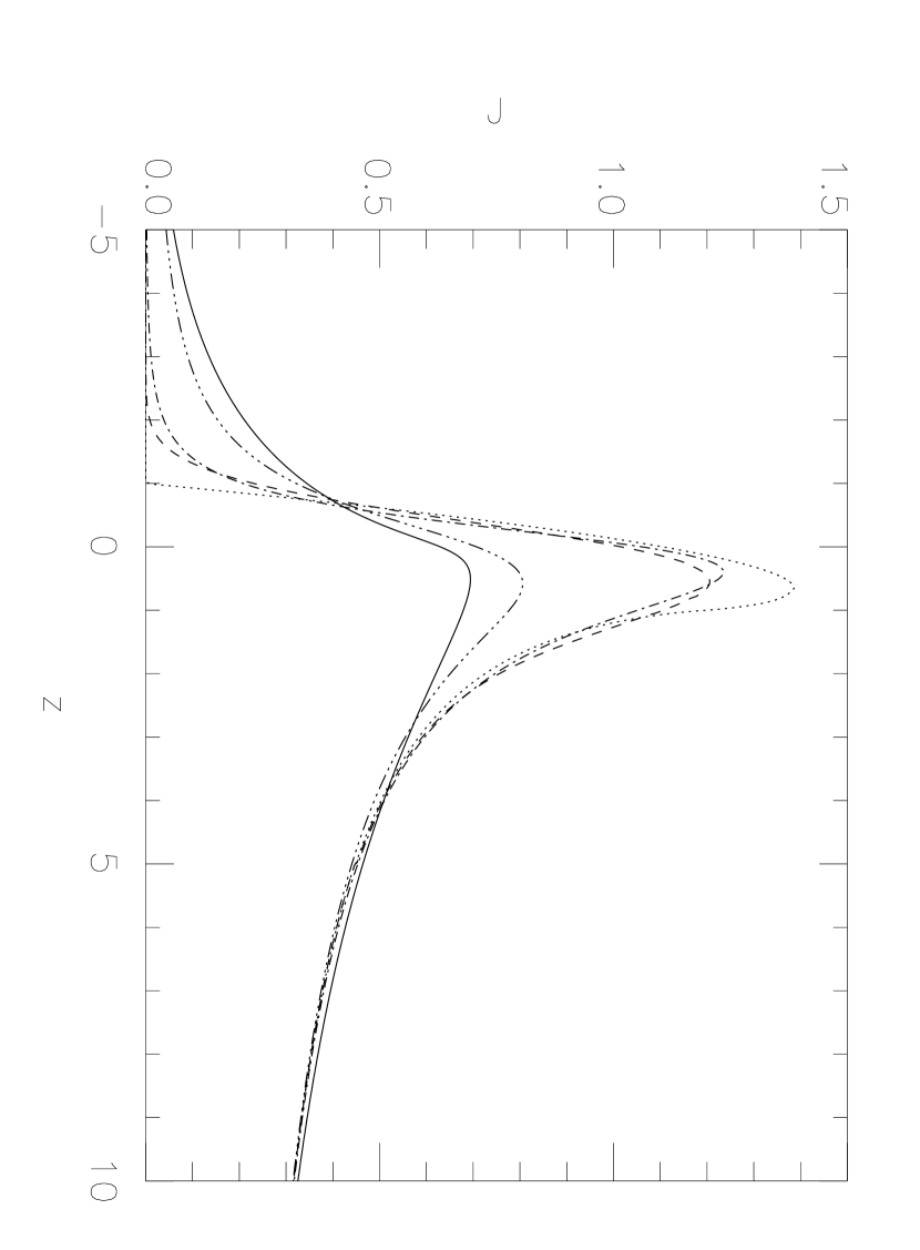
Figure 1:

Figure 2: (top)

Figure 2: (bottom)

Figure 3: (top)

Figure 3: (bottom)

Figure 4:

Table 1: Fits to the GLITP $V$-band light curve for Q2237+0305A.

Source model	$F_{0}$ (mJy)	$F_{C}$ (mJy)	$t_{0}$ (JD–2450000)	$\Delta t$ (days)	$\hat{\chi}^{2}(min)/\delta(min)$
Uniform	0.72	0.07	1489.6	$30.2^{+1.3}_{-1.3}$	1.33/1.62
Gaussian	0.71	0.09	1488.6	$31.0^{+8.3}_{-2.8}$	1.31/1.52
Power-law ($p_{V}$ = 5/2)	0.68	0.11	1486.1	$48.0^{+12.1}_{-8.4}$	1.18/0.88
Power-law ($p_{V}$ = 3/2)	0.65	0.19	1484.7	$33.1^{+8.3}_{-6.1}$	1.08/0.39
Standard	0.59	0.30	1480.6	$39.6^{+10.4}_{-9.5}$	0.99/0.05

Table 2: Fits to the GLITP $R$-band light curve for Q2237+0305A.

Source model	$F_{0}$ (mJy)	$F_{C}$ (mJy)	$t_{0}$ (JD–2450000)	$\Delta t$ (days)	$\hat{\chi}^{2}(min)/\delta(min)$
Uniform	1.28	0.09	1489.3	$30.7^{+1.4}_{-1.1}$	1.44/2.09
Gaussian	1.18	0.17	1483.7	$47.6^{+34.1}_{-9.0}$	1.30/1.42
Power-law ($p_{R}$ = 5/2)	1.14	0.20	1481.6	$65.5^{+34.4}_{-18.0}$	1.19/0.90
Power-law ($p_{R}$ = 3/2)	1.12	0.33	1481.4	$41.3^{+18.8}_{-10.9}$	1.12/0.57
Standard	1.06	0.46	1478.7	$43.0^{+15.0}_{-11.3}$	0.99/0.05

Table 3: Source size ratios and bounds on the dimension of the $V$-band and $R$-band sources.

Source model	$q=R_{V}/R_{R}$	$R_{V}(50\%)\times 10^{2}$ (pc)	$R_{R}(50\%)\times 10^{2}$ (pc)
Uniform	$0.98^{+0.05}_{-0.06}$	$<$ 0.044 (0.061)	$<$ 0.044 (0.063)
Gaussian	$0.65^{+0.21}_{-0.47}$	$<$ 0.065	$<$ 0.133
Power-law ($p$ = 5/2)	$0.73^{+0.27}_{-0.40}$	$<$ 0.091	$<$ 0.150
Power-law ($p$ = 3/2)	$0.80^{+0.29}_{-0.39}$	$<$ 0.140 (0.807)	$<$ 0.205 (1.172)
Standard	$0.92^{+0.34}_{-0.39}$	$<$ 0.234 (0.689)	$<$ 0.271 (0.800)

Table 4: Comparison between the standard fits to the GLITP and OGLE data.

Dataset	$F_{0}$ (mJy)	$F_{C}$ (mJy)	$t_{0}$ (JD–2450000)	$\Delta t$ (days)	$\hat{\chi}^{2}(min)$
GLITP	0.59	0.30	$1480.6^{+3.1}_{-3.2}$	$39.6^{+10.4}_{-9.5}$	0.99
OGLE99	0.72	0.20	$1487.6^{+1.0}_{-1.0}$	$14.3^{+3.4}_{-2.6}$	1.51
OGLE99-00	0.60	0.34	$1471.2^{+3.1}_{-2.8}$	$29.5^{+3.2}_{-3.1}$	7.49

References

- (1) Agol, E. & Krolik, J. 1999, ApJ, 524, 49
- (2) Alcalde, D., Mediavilla, E., Moreau, O. et al. 2002, ApJ, 572, 729
- (3) Chae, K-H., Turnshek, D. A. & Khersonsky, V. K. 1998, ApJ, 495, 609
- (4) Corrigan, R. T., Irwin, M. J., Arnaud, J. et al. 1991, AJ, 102, 34
- (5) Fluke, C. J. & Webster, R. L. 1999, MNRAS, 302, 68
- (6) Gaudi, B. S. & Petters, A. O. 2002, ApJ, in press
- (7) Grieger, B., Kayser, R. & Schramm, T. 1991, A&A, 252, 508
- (8) Grogin, N. A. & Narayan, R. 1996, ApJ, 464, 92
- (9) Irwin, M. J., Webster, R. L., Hewett, P. C. et al. 1989, AJ, 98, 1989
- (10) Jaroszyński, M., Wambsganss, J. & Paczyński, B. 1992, ApJ, 396, L65
- (11) Mediavilla, E., Arribas, S., Del Burgo, C. et al. 1998, ApJ, 503, L27
- (12) Mineshige, S. & Yonehara, A. 1999, PASJ, 51, 497
- (13) Østensen, R., Refsdal, S., Stabell, R. et al. 1996, A&A, 309, 59
- (14) Rauch, K. P. & Blandford, R. D. 1991, ApJ, 381, L39
- (15) Schmidt, R., Wambsganss, J., Kundić, T. et al. 2001, in ASP 237: Gravitational Lensing: Recent Progress and Future Goals, eds. T. Brainerd and C.S. Kochanek (San Francisco: ASP), 211
- (16) Schmidt, R., Webster, R. L. & Lewis, G. F. 1998, MNRAS, 295, 488
- (17) Schneider, P., Ehlers, J. & Falco, E. E. 1992, Gravitational Lenses (Berlin: Springer)
- (18) Schneider, P. & Weiss, A. 1987, A&A, 171, 49
- (19) Shakura, N. I. & Sunyaev, R. A. 1973, A&A, 24, 337
- (20) Shalyapin, V. N. 2001, AstL, 27, 150
- (21) Wambsganss, J. & Paczyński, B. 1994, AJ, 108, 1156
- (22) Wambsganss, J., Paczyński, B. & Schneider, P. 1990, ApJ, 358, L33
- (23) Webster, R. L., Ferguson, A. M. N., Corrigan, R. T. & Irwin, M. J. 1991, AJ, 102, 1939
- (24) Woźniak, P. R., Alard, C., Udalski, A. et al. 2000a, ApJ, 529, 88
- (25) Woźniak, P. R., Udalski, A., Szymański et al. 2000b, ApJ, 540, L65
- (26) Wyithe, J. S. B., Webster, R. L. & Turner, E. L. 1999, MNRAS, 309, 261
- (27) Wyithe, J. S. B., Webster, R. L. & Turner, E. L. 2000, MNRAS, 315, 51
- (28) Wyithe, J. S. B., Webster, R. L., Turner, E. L. & Mortlock, D. J. 2000, MNRAS, 315, 62
- (29) Yonehara, A. 2001, ApJ, 548, L127
- (30) Yonehara, A., Mineshige, S., Manmoto, T., Fukue, J., Umemura, M., & Turner, E. L. 1998, ApJ, 501, L41