Occultation and Microlensing

Abstract

Occultation and microlensing are different limits of the same phenomena of one body passing in front of another body. We derive a general exact analytic expression which describes both microlensing and occultation in the case of spherical bodies with a source of uniform brightness and a non-relativistic foreground body. We also compute numerically the case of a source with quadratic limb-darkening. In the limit that the gravitational deflection angle is comparable to the angular size of the foreground body, both microlensing and occultation occur as the objects align. Such events may be used to constrain the size ratio of the lens and source stars, the limb-darkening coefficients of the source star, and the surface gravity of the lens star (if the lens and source distances are known). Application of these results to microlensing during transits in binaries and giant-star microlensing are discussed. These results unify the microlensing and occultation limits and should be useful for rapid model fitting of microlensing, eclipse, and “microccultation” events.

1 Introduction

When two stars (or other bodies) come into close alignment on the sky, the foreground star may either eclipse or microlens the background star. As the stars align, if the angular size of the foreground star is much larger than its gravitational deflection angle, then the foreground star can eclipse; if the contrary is true then it can magnify. More precisely, gravitational lensing by a point mass produces two images of a distant object, one interior and one exterior to the Einstein radius in the lens plane, $R_{E}=[4R_{G}D_{L}(D_{S}-D_{L})/D_{S}]^{1/2}$ where $R_{G}=GM/c^{2}$ is the gravitational radius for a lens of mass $M$, and $D_{L,S}$ are the distances to the lens or source. Both images move toward the Einstein radius as the lens and source approach, so the outer image will be occulted during the approach if the radius of the lens is larger than the Einstein radius. The inner image, however, starts off near the origin and thus is occulted when the source is far from the lens. As the lens and source approach, the inner image can become unocculted if the lens is smaller than the Einstein radius (Figure 1). Occultation is most important in microlensing if $R_{E}\sim R_{L}$, where $R_{L}$ is the radius of the lens star (assumed to be spherical). In Galactic microlensing, typically $R_{L}\ll R_{E}$, so the occultation of the inner image occurs, but is usually rather faint. In special circumstances, such as in eclipsing binaries containing compact objects (Maeder, 1973; Marsh, 2001) or lensing by giant stars, $R_{L}\sim R_{E}$, so the effects of both microlensing and occultation must be included. This “microccultation” can show more varied behavior than the usual microlensing or occultation lightcurves and can be used to constrain the surface gravity of the lens star (Bromley, 1996).

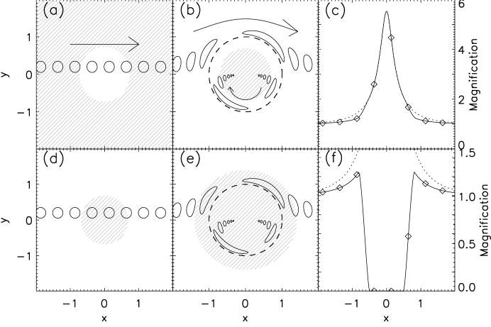
Figure 1: (a) Stars at various positions in source plane. Shaded region shows the area in which the inner image is occulted by the lens star for $r_{L}<1$, which is the region $\beta>\beta_{L}=1/r_{L}-r_{L}$. The axes have units of $R_{E}D_{S}/D_{L}$. (b) Images of the star in the image plane. The arrow is imaged as well for reference. The dashed line is $R_{E}$. (c) Magnification as a function of position - dotted line is without occultation, while solid line includes occultation. The symbols show the magnification of the source at the positions depicted in (a). (d)-(f) Same as (a)-(c), but for $r_{L}>1$. In this case, the inner image is fully occulted, and the shaded region in (d) shows where the outer image is occulted by the lens star.

Maeder (1973) and Marsh (2001) have carried out numerical computations of microccultation lightcurves. Here we present an exact analytic solution for the lightcurve of a uniform source which agrees with their work, and we present numerical calculations for limb-darkened sources. Bromley (1996) and Bozza et al. (2002) computed lightcurves for lensing events, treating the source as a point source, while the expressions presented here are valid for extended and limb-darkened sources as well. In section 2 we discuss microlensing and occultation of a point source. In section 3 we include the finite size of a uniform source. In section 4 we include the effects of limb-darkening numerically for microlensing and occultation. In section 5 we apply the results to several astrophysical cases of possible interest, namely white dwarf-main sequence binaries, microlensing in globular clusters, and microlensing by supergiants. In section 6 we summarize.

2 Point source

The lensing equation for a point source and point lens, neglecting diffraction and strong relativistic effects, is (Schneider et al., 1992)

$$\beta=\theta-{1\over\theta},$$ (1)

where $\theta$ and $\beta$ are the image and source position angles in units of $R_{E}/D_{L}$. In the limit that the source is much smaller than the Einstein radius and is not aligned with the lens, then the point-source magnification is an adequate approximation (Paczyński, 1986). Solving this equation, the image positions are

$$\theta_{\pm}={1\over 2}\left[\beta\pm\sqrt{4+\beta^{2}}\right],$$ (2)

where $\theta_{-}$ is the image interior to the Einstein radius and $\theta_{+}$ is the image exterior to the Einstein radius ($\left|\theta_{-}\right|<1$ and $\theta_{+}>1$). The magnifications of the images are

$$\mu^{p}_{\pm}={1\over 2}\left({2+\beta^{2}\over\beta\sqrt{4+\beta^{2}}}\pm 1\right),$$ (3)

or $\mu^{p}_{+}=(1-\theta_{+}^{-4})^{-1}$ and $\mu^{p}_{-}=(\theta_{-}^{-4}-1)^{-1}$.

If the size of the lens star is less than the size of the Einstein radius, $r_{L}=R_{L}/R_{E}<1$, then the inner image will be occulted for $\left|\theta_{-}\right|<r_{L}$. This corresponds to $\beta>r_{L}^{-1}-r_{L}$, which means that the inner image is occulted when the source is distant from the lens and unoccults when the source approaches the lens. The change in magnitude at the point of the occultation of the inner image is

$$\Delta m=-2.5\log{\left[1+{r_{L}^{4}\over 1+f(1-r_{L}^{4})}\right]},$$ (4)

where $f=F_{L}/F_{S}$ is the ratio of the flux from the lens to the unlensed flux from the source. In typical Galactic microlensing events, $r_{L}\ll 1$, so the inner image usually appears (unoccults) when the source is distant from the lens, so the change in magnitude is very small. However, if the images can be resolved directly and the demagnified inner image is brighter than the lens star, then appearance of the inner image might be detectable.

If the size of the lens star is greater than the Einstein radius, $r_{L}>1$, then the inner image is always occulted and the outer image will be occulted for $\theta_{+}<r_{L}$ which corresponds to $\beta<r_{L}-r_{L}^{-1}$. During occultation the source star disappears so that one can only see the lens star. Thus, the total magnification for microlensing of a point source is

$$\mu^{p}=\mu^{p}_{+}\Theta\left(r_{L}\beta-r_{L}^{2}+1\right)+\mu^{p}_{-}\Theta\left(1-r_{L}^{2}-r_{L}\beta\right),$$ (5)

where

$$\Theta(x)=\left\{\begin{array}[]{ll}1&x>0\\ 0&x\leq 0\\ \end{array}\right.$$ (6)

is the step-function. In the limit $r_{L}=0$, this reduces to the usual microlensing magnification (Paczyński, 1986), while in the limit $r_{L}\gg 1$, $\mu^{p}_{-}$ is negligible, $\mu^{p}_{+}\sim 1$, and occultation simply occurs when $\beta<r_{L}$.

At the point of occultation, $\beta=\pm\left(r_{L}^{-1}-r_{L}\right)$, and since $\beta$ can be measured from a fit to the microlensing lightcurve, one can measure $r_{L}$ (Bromley, 1996). The sign is determined by whether the image appears ($+$) or disappears ($-$) at the center of the event.

The average astrometric position of the images during the microlensing event is (Walker, 1995)

$$\Delta\theta={\mu^{p}_{+}\theta_{+}+\mu^{p}_{-}\theta_{-}\over\mu^{p}+f},$$ (7)

where the difference in image position is measured with respect to the position of the lens on the sky. When $r_{L}\ll 1$, then the change in position during occultation of the inner image is

$$\Delta\theta(r_{L})=-{r_{L}^{3}\over(1+f)^{2}}.$$ (8)

This has a weaker dependence on $r_{L}$ than the magnitude change, but will still be quite small unless $r_{L}\sim 1$. In the case where $r_{L}\gg 1$, then the source will be completely occulted, so the centroid change is simply

$$\Delta\theta(r_{L})={r_{L}\over f+1}.$$ (9)

The point source approximation has two limitations: during eclipse ingress or egress, the finite size of the source causes a smooth transition, and if the surface brightness of the source and lens are similar and $r_{L}\sim 1$, then the source must also have have a size similar to the Einstein radius to contribute a significant fraction of the flux. Thus, in the next section we derive a more general formula including the finite extent of the source.

3 Extended uniform source

In the case of a circular source with uniform surface brightness, the images may be partly or fully eclipsed by the lens star. The magnification (or dimming) is equal to the ratio of the unocculted area of the images to the area of the unlensed source since surface brightness is conserved during lensing. For a uniform source the area can be computed by integrating over the image boundaries using Stokes’ theorem (Gould and Gaucherel, 1997; Dominik, 1998). In the case of a point-mass lens, this integral can be solved analytically as first shown by Witt and Mao (1994) for $r_{L}=0$. For an extended source with normalized radius

$$r_{S}={R_{S}D_{L}\over R_{E}D_{S}},$$ (10)

it is more useful to define a two-dimensional lensing equation to integrate over the source. Witt and Mao (1994) define a complex lensing equation

$$\zeta=z-{1\over\bar{z}},$$ (11)

where $\zeta$ is the complex coordinate for the source plane in units of $R_{E}D_{S}/D_{L}$ and $z=x+iy$ is the complex coordinate for the lens plane in units of $R_{E}$. Comparing to equation 1, $|\beta|=|\zeta|$ and $|\theta|=|z|$.

We assume that the source has a uniform surface brightness in the region $\zeta_{0}+re^{i\phi}$ ($\zeta_{0}$ is real and positive) where $0\leq\phi<2\pi$ and $0\leq r\leq r_{S}$, while we assume that the lens is opaque in the region $0\leq|z|\leq r_{L}$. The solution for the image positions is

$$z_{\pm}={\zeta\over 2}\left[1\pm\sqrt{1+{4\over\zeta\bar{\zeta}}}\right],$$ (12)

which is the complex version of equation 2. The lensing magnification for a uniform source is simply the ratio of the area of the lensed images to the area of the source. The integral over area can be converted to an integral over the source boundary using Stokes’ theorem (Gould and Gaucherel, 1997), giving

$$\mu_{\pm}=\pm{1\over\pi r_{S}^{2}}\int d\phi|z_{\pm}|^{2}{\partial\Psi\over\partial\phi},$$ (13)

where $\Psi=\cot^{-1}\left({\zeta_{0}r_{S}^{-1}\csc{\phi}+\cot{\phi}}\right)$ is the position angle of the image. The total magnification is

$$\mu=\mu_{+}+\mu_{-}.$$ (14)

In case of a finite-sized lens, $z_{\pm}$ should be replaced in the integrand with $r_{L}e^{i\Psi}$ whenever $|z_{\pm}|\leq r_{L}$. In other words, when an image is partially occulted, then the inner boundary is given by the edge of the lens, while the outer boundary is given by the edge of the outer image.

There are several different cases to consider:

1. $r_{S}=0$: Point source (equation 5);

2. $r_{S}>0$, $r_{L}=0$: Extended source, unocculted (Witt and Mao, 1994);

3. $r_{S}>0$, $1>r_{L}>0$: Extended source, inner image may be partly occulted, outer image unocculted;

4. $r_{S}>0$, $r_{L}>1$: Extended source, inner image fully occulted, outer image may be partly occulted.

The expressions for $\mu_{\pm}$ in each of these cases are summarized in Tables 1 and 2, where $p,e,$ and $o$ superscripts refer to the point-source magnification (Paczyński, 1986), extended-source magnification (Witt and Mao, 1994), or occulted-extended source magnification (below), respectively and $\beta_{L}=|r_{L}^{-1}-r_{L}|$. Each of the magnification expressions in Tables 1 and 2 are given in equations 5 and 17-40, with the the range of the variables for which the functions apply given in the columns.

As an example of how the computation proceeds, we consider the case in which $r_{L}>1$ and the source overlaps the shadow of the lens (for example, the source in Figure 1(d) at $x=0.6$). In this case the inner image is completely occulted while the outer image is partially occulted, so we must integrate equation 13 for $\phi$ between $\pm\chi=\pm\cos^{-1}\left[\left(\beta_{L}^{2}-r_{S}^{2}-\zeta_{0}^{2}\right)/\left(2r_{S}\zeta_{0}\right)\right]$. This gives an area which is between the outer edge of the source image and origin, so we need to subtract off the area within the shadow which is $r_{L}^{2}\phi_{2}=r_{L}^{2}\cos^{-1}\left[\left(r_{S}^{2}-\beta_{L}^{2}-\zeta_{0}^{2}\right)/\left(2\beta_{L}\zeta_{0}\right)\right]$. Thus,

$$\mu^{o}_{+}={1\over\pi r_{S}^{2}}\int_{-\chi}^{\chi}d\phi|z_{\pm}|^{2}{\partial\Psi\over\partial\phi}-{\phi_{2}r_{L}^{2}\over\pi r_{S}^{2}}.$$ (15)

Making the substitution $u=\beta^{2}=\zeta_{0}^{2}+r_{S}^{2}+2\zeta_{0}r_{S}\cos{\phi}$, this equation is

$$\mu^{o}_{+}={1\over 4\pi r_{S}^{2}}\int_{\beta_{L}^{2}}^{u_{2}}du{(u-u_{3})\left(1+2u^{-1}+\sqrt{4+u\over u}\right)\over\left[(u_{2}-u)(u-u_{1})\right]^{1/2}}-{\phi_{2}r_{L}^{2}\over\pi r_{S}^{2}},$$ (16)

where $u_{1}$, $u_{2}$, and $u_{3}$ are defined below. The integral can be reduced to elliptic integrals as given below.

For an extended source ($r_{S}>0$), the magnification of the inner image when $1>r_{L}>0$ is given by:

$$\mu^{o}_{-} = {\Theta(r_{S}-\zeta_{0})\over r_{S}^{2}}-{1\over 4\pi r_{S}^{2}}\left[\vphantom{\left(\sqrt{1+4/u_{0}}-1\right)}2(1+r_{S}^{2})\phi_{1}-4sgn(u_{3})\phi_{0}+4r_{L}^{2}\phi_{2}\right.$$ (17)

$$+ \left.\sqrt{(u_{2}-u_{0})(u_{0}-u_{1})}\left(\sqrt{1+4/u_{0}}-1\right)-G(\phi_{0})\right],$$ (18)

where

$$G(\phi) = {1\over\sqrt{u_{2}(4+u_{1})}}\left[\vphantom{r_{S}^{2}}u_{2}(4+u_{1})E(\phi,k_{1})-(u_{1}u_{2}+8u_{3})F(\phi,k_{1})\right.$$ (19)

$$+ \left.4u_{1}(1+r_{S}^{2})\Pi(\phi,n,k_{1})\right],$$ (20)

$F,E,$ and $\Pi$ are elliptic integrals of the first, second and third kinds (Gradshteyn and Ryzhik, 1994), $sgn(x)$ chooses the sign of $x$, and the other variables are

$$u_{0} = \beta_{L}^{2}$$ (21)

$$u_{1} = (\zeta_{0}-r_{S})^{2}$$ (22)

$$u_{2} = (\zeta_{0}+r_{S})^{2}$$ (23)

$$u_{3} = \zeta_{0}^{2}-r_{S}^{2}$$ (24)

$$\phi_{0} = \cos^{-1}{\sqrt{u_{1}(u_{2}-u_{0})\over u_{0}(u_{2}-u_{1})}}$$ (25)

$$\phi_{1} = \cos^{-1}{\left[u_{1}+u_{2}-2u_{0}\over u_{2}-u_{1}\right]}$$ (26)

$$\phi_{2} = \cos^{-1}{\left[u_{3}+u_{0}\over 2\zeta_{0}u_{0}^{1/2}\right]}$$ (27)

$$n = 1-{u_{1}\over u_{2}}$$ (28)

$$k_{1}^{2} = {4(u_{2}-u_{1})\over u_{2}(4+u_{1})}.$$ (29)

In the special case that $\zeta_{0}=r_{S}$, the magnification of the inner image becomes

$$\mu_{-}^{o,*} = \mu_{-}^{e,*}+{1\over\pi r_{S}^{2}}\left[\vphantom{\beta_{L}\over 2r_{S}}\left(1+r_{S}^{2}-r_{L}^{2}\right)\cos^{-1}{\beta_{L}\over 2r_{S}}+{v_{2}\over 4}(\beta_{L}-v_{1})\right.$$ (30)

$$- \left.(1+r_{S}^{2})\tan^{-1}{v_{2}\over v_{1}}\right]$$ (31)

where

$$v_{1} = \sqrt{4+\beta_{L}^{2}}$$ (32)

$$v_{2} = \sqrt{4r_{S}^{2}-\beta_{L}^{2}},$$ (33)

and

$$\mu_{\pm}^{e,*}={1\over\pi r_{S}^{2}}\left[r_{S}+(1+r_{S})^{2}\tan^{-1}{r_{S}}\right]\pm{1\over 2}.$$ (34)

which is the magnification of the unocculted images when $\zeta_{0}=r_{S}$.

When $r_{L}>1$, then the outer image can be occulted. The magnification in this case is given by:

$$\mu_{+}^{o} = {1\over 4\pi r_{S}^{2}}\left[2(1+r_{S}^{2})\psi_{2}-4sgn(u_{3})\psi_{1}-4r_{L}^{2}\phi_{2}\right.$$ (35)

$$+ \left.\sqrt{(u_{2}-u_{0})(u_{0}-u_{1})}\left(\sqrt{u_{0}/(4+u_{0})}+1\right)+G(\psi_{0})\right],$$ (36)

where

$$\psi_{0} = \cos^{-1}{\sqrt{(u_{0}-u_{1})(4+u_{2})\over(4+u_{0})(u_{2}-u_{1})}},$$ (37)

$$\psi_{1} = {\pi\over 2}-\phi_{0},$$ (38)

$$\psi_{2} = \pi-\phi_{1}+2\cos^{-1}\sqrt{u_{0}(4+u_{0})\over u_{0}(4+u_{1}+u_{2})-u_{1}u_{2}},$$ (39)

and the other variables are as in equation 21.

When the inner or outer images are unocculted, then the magnification is

$$\mu^{e}_{-} = {G(\pi/2)\over 4\pi r_{S}^{2}}-{1\over 2},$$ (40)

$$\mu^{e}_{+} = {G(\pi/2)\over 4\pi r_{S}^{2}}+{1\over 2},$$ (41)

which agrees with the expression of (Witt and Mao, 1994). In principle, one could also compute the image centroid for the source including occultation (as done by Witt, 1995).

We now provide several graphical examples of these equations. Figure 2 shows the magnification for a source with $r_{L}=0.9$ and $r_{S}=0.25$, compared with cases in which either $r_{L}=0$ or $r_{S}=0$. In all three cases the outer image is unobscured, but the inner image appears when the source approaches the lens. In the point source case, the appearance is abrupt and creates a strong brightening, while for the extended source the appearance is more gradual.

Fig. 2. – Magnification for $r_{S}=0.25$, $r_{L}=0.9$ (solid), $r_{S}=0$, $r_{L}=0.9$ (dotted - in this case the horizontal axis is scaled by $r_{S}=0.25$ for comparison), $r_{S}=0.25$, $r_{L}=0$ (dashed).

Figure 3 shows the magnification for a source with $r_{L}=1.1$ and $r_{S}=0.25$, compared with cases in which either $r_{L}=0$ or $r_{S}=0$. The finite size of the lens and the source creates both magnification and occultation, but the magnification wins out ($\mu>1$) in this case. In all three cases the inner image is obscured, while the outer image can be obscured when the source approaches the lens. In the point source case the occultation is abrupt and results in disappearance of the background source.

Fig. 3. – Magnification for $r_{S}=0.25$, $r_{L}=0.9$ (solid), $r_{S}=0$, $r_{L}=0.9$ (dotted - in this case the horizontal axis is scaled by $r_{S}=0.25$ for comparison), $r_{S}=0.25$, $r_{L}=0$ (dashed).

For the case of $r_{S}=1$, we show several different values of $r_{L}$ in Figure 4. In all cases with finite $r_{L}$ the magnification shows a much flatter profile near the origin than for the $r_{L}=0$ case. In the limit $r_{L}\ll 1$ the lightcurve approaches that of extended-source microlensing, while for $r_{L}\gg 1$ approaches the limit of occultation.

Fig. 4. – Magnification for $r_{S}=1$ and $r_{L}=0.8,0.95,1.05,1.2,1.8$ (solid lines from top to bottom); $r_{L}=0$ is dashed line.

Figure 5 shows magnification for different source sizes, but fixed lens size $r_{L}=0.95$. The smallest sources show broad sloping wings indicative of the appearance of the second image; in the smallest case the source becomes completely revealed near the origin. For the largest cases the magnification shows a sharper slope near $\zeta_{0}=r_{S}$ than in the $r_{L}=0$ case.

Fig. 5. – Magnification for $r_{S}={1\over 16},{1\over 8},{1\over 4},{1\over 2},1,2$ from top to bottom. Solid lines show $r_{L}=0.95$, while dashed lines show $r_{L}=0$.

A uniform source causes rather sharp features in the lightcurve during the ingress and egress of the occultation, and leads to flatter lightcurves during transit. However, a limb-darkened source has a smoother ingress/egress and has curvature during a transit. Thus, in the next section we consider microlensing and occultation of a limb-darkened source.

4 Limb Darkening

Limb darkening causes a star to be more centrally peaked in brightness compared to a uniform source. This leads to larger magnification during microlensing or larger dimming during transit/occultation. Thus, including limb-darkening is important for computing accurate microlensing/occultation lightcurves. Describing limb-darkening with a quadratic law

$${I(r)\over I(0)} = 1-\gamma_{1}(1-\sigma)-\gamma_{2}(1-\sigma)^{2},$$ (42)

$$\sigma = \sqrt{1-\left({r\over r_{S}}\right)^{2}},$$ (43)

where $\gamma_{1}+\gamma_{2}<1$, leads to a magnification of

$$\mu(r_{L},r_{S},\zeta_{0},\gamma_{1},\gamma_{2})=\left[\int_{0}^{r_{S}}drI(r)\right]^{-1}\int_{0}^{r_{S}}drI(r){d\mu r^{2}\over dr},$$ (44)

where $\mu(r)$ can be computed from the expressions in the previous section (replacing $r_{S}$ with $r$). We could use a more accurate limb-darkening formula, but rely on a quadratic law for simplicity. Given the complicated dependence of the magnification on the radius, this integral is best done numerically using a finite-difference approximation for the derivative of the uniform magnification. An example is shown in Figure 6 - in this case the dip during occultation is deeper due to limb-darkening since the source is brighter at the center, and thus more flux is lost, and the magnification decreases toward the origin rather than increasing as in the uniform source case. Both the uniform and the limb-darkened cases are shallower when compared to the pure occultation case due to magnification of the background source. A second example is shown in Figure 7. In this case the limb-darkening causes a weaker magnification as the outer limb is magnified, while the peak is increased due to the more concentrated brightness. In the special case that $\zeta_{0}=0$, the integral is tractable analytically as follows, and is shown as the solid dots in Figures 6 and 7.

Fig. 6. – Magnification for $r_{S}=5$ and $r_{L}=1.5$. The solid line is limb-darkened with $\gamma_{1}=\gamma_{2}=0.3$ (equation 44), while the dashed line is a uniform source (equation 14, Tables 1 and 2). The dash-dot line shows a uniform source and lens of the same size ratio but neglecting lensing, while the dotted line is for a limb-darkened source neglecting lensing.

For $r_{L}>0$ and $r_{S}>\beta_{L}$, the magnification for a limb-darkened source at $\zeta_{0}=0$ becomes

$$\mu = {\sqrt{4+r_{S}^{2}}\over 6\Omega r_{S}^{3}}\left[\alpha_{1}\left((2+r_{S}^{2})E(\phi_{3},k_{2})-2F(\phi_{3},k_{2})\right)+\alpha_{2}r_{S}\right]$$ (45)

$$+ {1\over 6\Omega r_{S}^{3}}\left(s\beta_{L}(4+\beta_{L}^{2})^{1\over 2}+\alpha_{3}\right)\left(\alpha_{1}\sqrt{\alpha_{3}}+\alpha_{2}-{3\gamma_{2}\over 2r_{S}}\alpha_{3}\right)$$ (46)

$$+ {2\gamma_{2}\over r_{S}^{4}\Omega}\left[{\alpha_{3}\over 8}(2+r_{S}^{2})+\sinh^{-1}\left({r_{S}\over 2}\right)+\sinh^{-1}\left({s\beta_{L}\over 2}\right)\right],$$ (47)

where

$$\alpha_{1} = 2(\gamma_{1}+2\gamma_{2}),$$ (48)

$$\alpha_{2} = 3(1-\gamma_{1}-\gamma_{2})r_{S}-{3\gamma_{2}\over 2r_{S}}(2+r_{S}^{2}),$$ (49)

$$\alpha_{3} = r_{S}^{2}-\beta_{L}^{2},$$ (50)

$$\Omega = 1-\gamma_{1}/3-\gamma_{2}/6,$$ (51)

$$\phi_{3} = \cos^{-1}\left(-s{\beta_{L}\over r_{S}}\right),$$ (52)

$$s = sgn(1-r_{L}),$$ (53)

$$k_{2}^{2} = {r_{S}^{2}\over 4+r_{S}^{2}}.$$ (54)

When $\phi_{3}>\pi/2$, then $E(\phi_{3},k_{2})=2E(k_{2})-E(\pi-\phi_{3},k_{2})$ and $F(\phi_{3},k_{2})=2K(k_{2})-F(\pi-\phi_{3},k_{2})$. For $r_{L}<1$ and $r_{S}<\beta_{L}$, the inner image is unocculted (the latter is always true for $r_{L}=0$), and $\beta_{L}$ should be replaced by $r_{S}$ in equations 45 and 48 to give

$$\mu={1\over\Omega r_{S}^{2}}\left[{\alpha_{1}\over 3k_{2}}\left((2+r_{S}^{2})E(k_{2})-2K(k_{2})\right)+{\alpha_{2}r_{S}\over 3k_{2}}+{4\gamma_{2}\over r_{S}^{2}}\sinh^{-1}\left({r_{S}\over 2}\right)\right].$$ (55)

For $\gamma_{2}=0$, this expression agrees with equation (A6) in Witt (1995).

Fig. 7. – Magnification for $r_{S}=5$ and $r_{L}=0.5$. The solid line is limb-darkened with $\gamma_{1}=\gamma_{2}=0.3$, while the dashed line is a uniform source.

In the occultation limit when the Einstein radius is small, $R_{E}\ll R_{L},R_{S}$, then the lightcurve can be described by occultation only. We can include limb-darkening exactly in this case (Mandel & Agol, 2002). An example is shown in Figure 6 of the difference between occulting and microcculting lightcurves.

5 Discussion

The equations for microccultation are most relevant for equality of the Einstein radius and lens radius which occurs if $D\equiv D_{L}(D_{S}-D_{L})/D_{S}=R_{L}^{2}/(4R_{G})$. We compute $D$ for several interesting objects in Table 3 (not to be confused with their actual distances), including a white dwarf (Sirius B), brown dwarf (Gliese 229b), red giant (Capella), blue supergiant (Rigel), yellow supergiant (Deneb), and red supergiant (Betelgeuse). Application of the microccultation equations to white dwarfs, brown-dwarfs, nearby supergiants, and giants in globular clusters are discussed next.

White dwarfs in eclipsing binaries are the most likely location to see microccultation (Maeder, 1973; Marsh, 2001). Known white-dwarf binaries which transit their companions have small semi-major axes (likely a selection effect), and thus small Einstein radii, changing the depth of transit by only a few percent (Marsh, 2001). Due to common-envelope evolution, white-dwarf binaries have typical semi-major axes $a\sim 0.1$ AU and masses of $0.5M_{\odot}$, so $R_{E}\sim 7\times 10^{8}{\rm cm}(M/0.5M_{\odot})^{1/2}(a/0.1{\rm AU})^{1/2}$. This is comparable to the size of white dwarfs, $\sim 10^{9}$ cm, so both occultation and microlensing will be important. Farmer et al. (2002) apply the formulae derived here to estimate how many white dwarfs may be found in transit searches for extrasolar planets. For example, the Kepler survey (Koch et al., 1998) may find $\sim 10-100$ white dwarfs, comparable to the expected number of terrestrial planets. White dwarf transit events will require including both lensing and occultation in modeling the lightcurves.

Though smaller in mass, brown dwarfs in eclipsing binaries may have some observable microlensing effects during eclipse. As gas planets and brown dwarfs have very similar sizes, their transits of companion stars may look quite similar. However, in the limit of a large source the depth of the transit scales as $1+2(R_{E}/R_{S})^{2}-(R_{L}/R_{S})^{2}$ (for a uniform source), so brown dwarfs will have a transit of smaller depth since $R_{E}$ is larger. This will affect the measurement of limb-darkening which also changes the depth of the transit (equation 45). In the case of a 0.05 $M_{\odot}$ brown dwarf with radius $0.1R_{\odot}$ in orbit at 1 AU about a G-type star, $r_{L}=10$ and $r_{S}=10^{2}$. Thus, the transit depth differs by $2\times 10^{-4}$ from a $10^{-3}M_{\odot}$ planet of the same radius. Such photometric precision can be obtained with HST (Brown et al., 2001) and other planned satellites, and will be indicated by a slight brightening outside of the transit (Figure 6). The difference can be much larger, $\sim 1$%, if the primary is also a brown dwarf.

Lensing events caused by nearby stars may also show the signs of both microlensing and occultation. The most extreme case is the star Betelgeuse which has a distance of $\sim 125$ pc and a mass of $\sim 20M_{\odot}$, giving an Einstein radius of $7\times 10^{13}$ cm for sources at much larger distance. This is only slightly larger than the size of Betelgeuse, $\sim 4\times 10^{13}$ cm, so that distant stars passing behind Betelgeuse would create two visible images as they approach; a full occultation would never occur (unless the mass of Betelgeuse were much smaller). Distant galaxies would create an Einstein ring surrounding the star with the center occulted. The challenge involved in carrying out such an observation is resolving a faint background source from the bright foreground star and waiting long enough for Betelgeuse to pass in front of a star or galaxy. In every microlensing event an occultation should occur when $\beta=\beta_{L}$. Since this usually leads to a demagnified image, extremely accurate photometry is necessary to see an occultation event.

A final application of the microccultation equations is to giant stars acting as lenses in globular clusters. There are about $3\times 10^{5}$ evolved giant stars in Milky Way globular clusters. For a giant star at the clump with a mass of $1M_{\odot}$, the Einstein radius for a separation of 1 pc is $\sim 20R_{\odot}$, comparable to the size of the star, $\sim 20R_{\odot}$. If the relative velocity is $\sim 10$ km/s then red giants in globular clusters cover about $3\times 10^{31}$ cm² yr^-1 which is about $10^{-8}$ of the total area in globular clusters. Thus, about $10^{8}$ stars in globular clusters must be monitored to find a single red giant transit event per year and a typical event will last about one month. A lightcurve of a lensing event by a red giant in a globular cluster would allow one to measure $r_{L}$ and $r_{S}$, as well as $\gamma_{1}$ and $\gamma_{2}$ for the source star. Since the Einstein radius in this case is $R_{E}=\left[4GMc^{-2}D\right]^{1/2}$ where $D$ is the separation of the lenses in the cluster, one can estimate the surface gravity of the lens giant, $g=GM/R_{L}^{2}\sim c^{2}/(4D)$ (Bromley, 1996), given that $D$ will be of order the scale-length of the globular cluster.

6 Conclusions

We have computed exact formulae for lensing of a uniform extended source by an opaque, spherical lens (with escape velocity much smaller than $c$). The formulae only differ significantly from the usual occultation or microlensing formulae in the limit that $R_{L}\sim R_{E}$, which may be relevant for lensing by white dwarfs in binaries or lensing by giant stars. Small deviations due to lensing in eclipsing brown-dwarf binaries may be detectable with very precise photometry, which may be another application of the expressions derived here. A code written in IDL which carries out the calculations presented here can be downloaded from http://www.astro.washington.edu/agol/.

References

- Bozza et al. (2002) Bozza, V., Jetzer, Ph.2, Mancini, L., & Scarpetta, G., 2002, A&A, 382, 6
- Bromley (1996) Bromley, B., 1996, ApJ, 467, 537
- Brown et al. (2001) Brown, T. M., Charbonneau, D., Gilliland, R. L., Noyes, R. W., & Burrows, A., 2001, ApJ, 552, 699
- Dominik (1998) Dominik, M., 1998, A&A, 333, L79
- Farmer et al. (2002) Farmer, A., Agol, E., & Wyithe, S., 2002, in preparation
- Gradshteyn and Ryzhik (1994) Gradshteyn, I. S. & Ryzhik, I. M., 1994, (New York: Academic Press)
- Gould and Gaucherel (1997) Gould, A. & Gaucherel, C., 1997, ApJ, 477, 580
- Koch et al. (1998) Koch, D., Borucki, W., Webster, L., Dunham, E., Jenkins,J., Marriott, J. & Reitsema, H., 1998, SPIE Conference 3356, Space Telescopes and Instruments, p. 599
- Maeder (1973) Maeder, A., 1973, A&A, 26, 215
- Mandel & Agol (2002) Mandel, K. & Agol, E., 2002, in preparation
- Marsh (2001) Marsh, T. R., 2001, MNRAS, 324, 547
- Merrill (1950) Merrill, J. E., 1950, Contributions from the Princeton University Observatory, No. 23
- Paczyński (1986) Paczyński, B., 1986, ApJ, 304, 1
- Schneider et al. (1992) Schneider, P., Ehlers, J., & Falco, E. E., 1992, Gravitational Lenses (New York: Springer)
- Walker (1995) Walker, M., 1995, ApJ, 453, 37
- Witt and Mao (1994) Witt, H. J. & Mao, S., 1994, ApJ, 430, 505
- Witt (1995) Witt, H. J., 1995, ApJ, 449, 42