Detecting Radio Emission from Cosmic Ray Air Showers and Neutrinos with a Digital Radio Telescope

Abstract

We discuss the possibilities of measuring ultra-high energy cosmic rays and neutrinos with radio techniques. We review a few of the properties of radio emission from cosmic ray air showers and show how these properties can be explained by coherent “geosynchrotron” emission from electron-positron pairs in the shower as they move through the geomagnetic field. This should allow one to use the radio emission as a useful diagnostic tool for cosmic ray research. A new generation of digital telescopes will make it possible to study this radio emission in greater detail. For example, the planned Low-Frequency Array (LOFAR), operating at 10-200 MHz, will be an instrument uniquely suited to study extensive air showers and even detect neutrino-induced showers on the moon. We discuss sensitivities, count rates and possible detection algorithms for LOFAR and a currently funded prototype station LOPES. This should also be applicable to other future digital radio telescopes such as the Square-Kilometer-Array (SKA). LOFAR will be capable of detecting air-shower radio emission from $>2\cdot 10^{14}$ eV to $\sim 10^{20}$ eV. The technique could be easily extended to include air shower arrays consisting of particle detectors (KASCADE, Auger), thus providing crucial additional information for obtaining energy and chemical composition of cosmic rays. It also has the potential to extend the cosmic ray search well beyond an energy of $10^{21}$ eV if isotropic radio signatures can be found. Other issues that LOFAR can address are to determine the neutral component of the cosmic ray spectrum, possibly look for neutron bursts, and do actual cosmic ray astronomy.

1 Introduction

A standard method to observe energetic cosmic rays is simply an array of particle detectors on the ground measuring either the energetic muons or electrons in the shower pancake. Since only a small fraction of the total number of particles in the shower are intercepted by the ground array, the conversion from number of particles received to primary particle energy is not really straight forward. Very useful additional information for energy calibration and particle track recovery of air showers can therefore be gained by observing radiation emitted from the secondary particles as the shower evolves. Such radiation is for example Cherenkov radiation, as observed in the CASA-MIA-DICE experiment, or fluorescence light from nitrogen molecules in the atmosphere, as seen by the Fly’s Eye detector HiRes and others. So far this emission is only detected in the optical and hence requires clear and moonless dark skies far outside major cities. This gives a duty-cycle of typically 10%.

Radio emission might provide an alternative method for doing such observations including detecting neutrino-induced showers at a higher duty cycle. This becomes particularly relevant since a new generation of digital radio telescopes – designed primarily for astronomical purposes – promises a whole new approach to measuring air showers.

2 Radio properties of extensive air showers

Radio emission from extensive air showers (EAS) was discovered for the first time by Jelley and co-workers in 1965 at a frequency of 44 MHz. They used an array of dipole antennas in coincidence with Geiger counters. The results were soon verified and emission from 2 MHz up to 520 MHz was found in a flurry of activities in the late 1960s. These activities ceased almost completely in the subsequent years due to several reasons: difficulty with radio interference, uncertainty about the interpretation of experimental results, and the success of other techniques for air shower measurements.

The radio properties of air showers are summarized in an excellent and extensive review by Allan (1971). The main result of this review can be summarized by an approximate formula relating the received time-integrated voltage of air shower radio pulses to various parameters, where we also include the presumed frequency scaling:

$$\epsilon_{\nu} = 13\,~{}\mu{\rm V}{\rm~{}m}^{-1}{\rm~{}MHz}^{-1}\left({E_{\rm p}\over 10^{17}~{}{\rm eV}}\right)\left({\sin\alpha\,\cos\,\theta\over\sin 45^{\circ}\,\cos 30^{\circ}}\right)$$ (1)

$$\times \exp\left({-R\over R_{0}(\nu,\theta)}\right)\left({\nu\over 50~{}{\rm MHz}}\right)^{-1}.$$

Here $E_{\rm p}$ is the primary particle energy, $R$ is the offset from the shower center and $R_{0}$ is around 110 m, $\theta$ is the zenith angle, $\alpha$ is the angle of the shower axis with respect to the geomagnetic field, and $\nu$ is the observing frequency (see also Allan et al. 1970; Hough & Prescott 1970). One has to be careful, however, since in later work by the Haverah Park group consistently lower values ($1-5\mu{\rm V}{\rm~{}m}^{-1}{\rm~{}MHz}^{-1}$ at $\nu=60$ MHz and $E_{\rm p}=10^{17}$ eV) have been claimed (e.g., Prah 1971; Sun 1975). Some of these discrepancies may be blamed on sytematic errors in the determination of $E_{\rm p}$ which was used to normalize the results.

The voltage of the unresolved pulse in the coherent regime ($\nu\leq 100~{}$MHz) can be converted into an “equivalent flux density” in commonly used radio astronomical units, i.e. Jansky. Since the conversion of pulsed emission – which contains an inherent time scale – to a flux density is not straightforward, we define as the equivalent flux density $S_{\nu}$ of a pulse the flux density of a steady continuum source of the same spectrum which deposits the same energy $E=S_{\nu}\Delta T\Delta\nu A_{\rm eff}$ in the antenna during the bandwidth-limited time interval $\Delta t$ as the pulse. Starting from the Poynting vector, we can define

$$S_{\nu}=\epsilon_{\nu}^{2}\epsilon_{0}c/\Delta t=0.27\,{\rm MJy}\;\left({\epsilon_{\nu}\over\mu{\rm V}~{}{\rm m}^{-1}{\rm~{}MHz}^{-1}}\right)^{2}\left({\Delta t\over\mu s}\right)^{-1}.$$ (2)

The observed pulse duration is $\Delta t\sim 1/\Delta\nu$ if the measurement is bandwidth-limited. In the earlier measurements the pulses were always unresolved when observing with $\Delta\nu\simeq 1$ MHz.

The formula in Eq. 1 was determined experimentally from data in the energy regime $10^{16}\;{\rm eV}\,<E_{\rm p}<10^{18}$ eV. The flux density around 100 MHz seems to depend on primary particle energy as $S_{\nu}\propto E_{\rm p}^{2}$ (Hough & Prescott 1970; Vernov et al. 1968; Fig. 1) as expected for coherent emission (see below). This dependency is, however, not yet undoubtedly established, since a few earlier measurements apparently found somewhat flatter power-laws (Barker et al. 1967 as quoted in Allan 1971).

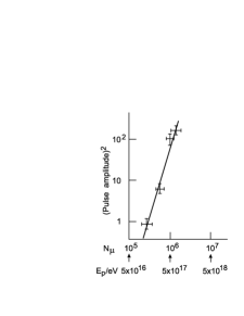
Figure 1: The dependence of EAS radio flux on the primary particle energy as measured by Vernov et al. (1968) following roughly a $E_{\rm p}^{2}$ power law. Some earlier papers found somewhat flatter dependencies.

The spectral form of the radio emission was claimed to be valid in the range 2 MHz $\leq\nu\leq$ 520 MHz but in general is also fairly uncertain. In fact, only very few data on the spectral dependence of EAS radio emission exist (e.g., Spencer 1969). Figure 2 shows a tentative EAS radio spectrum with a $\nu^{-2}$ dependence for the flux density ($\nu^{-1}$ dependence for the voltage). The 2 MHz data point was made with a different experiment and there is a real possibility that the spectrum is actually flat between 10-100 MHz (see Sun 1975; Datta et al. 2000). The polarization of the emission could be fairly high and is basically along the geomagnetic E-W direction (Allan, Neat, & Jones 1967; Sun 1975) which strongly supports an emission mechanism related to the geomagnetic field. Most recent attempts to measure the emission with a single antenna (Green et al.2002) produced only upper limits consistent with the older measurements.

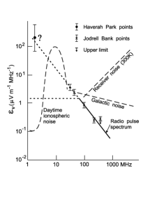
Figure 2: A tentative radio pulse spectrum (from Allan 1971 and Spencer 1969) from 2 MHz to 520 MHz for particles normalized to $E_{\rm p}=10^{17}$ eV. This has to be squared to get a flux density spectrum. The data are not simultaneous. The 2 MHz point was later questioned and evidence for a flattening of the spectrum (lower short-dashed line) below 100 MHz was found (e.g. Sun 1975). Various noise contributions as a function of frequency are also shown.

Finally, one needs to consider the spatial structure of the radio pulse. The current data strongly support the idea that the emission is not isotropic but is highly beamed in the shower direction. Figure 3 shows EAS radio pulse amplitude measurements as a function of distance $R$ from the shower axis – the flux density drops quickly with offset from the center of the shower. The characteristic radius of the beam is of order 100 meter for a $10^{17}$ eV vertical shower, with the emission presumably originating at 5-7 km distance above an observer at sea level. The implied angular diameter of the beam is thus $\Theta\simeq 0.2/6=1.9^{\circ}$.

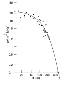
Figure 3: Normalized radio pulse amplitudes in $\mu$V m^-1 MHz^-1 at 55 MHz as a function of lateral distance $R$ in meters from the shower axis. Each data point corresponds to one measured cosmic ray event. The amplitudes were normalized to a reference energy of $E_{\rm p}=10^{17}$ eV assuming the above mentioned linear dependence of voltage on primary particle energy. The measurements were made for zenith angles $\theta<30^{\circ}$. Crosses and dots represent different particle energy bins between $10^{17}$ eV and $10^{18}$ eV. The plus sign at 500 meters marks a single $10^{19}$ eV event (from Allan 1971).

3 Emission process

Experiments have clearly established that cosmic ray air showers produce radio pulses. The original motivation was due to a suggestion from Askaryan (1962) who argued that annihilation of positrons would lead to a negative charge excess in the shower, thus producing Cherenkov radiation as it rushes through the atmosphere. At radio frequencies the wavelength of the emission is larger than the size of the emitting region and the emission should be coherent. The radio flux would then grow quadratically with the number of particles rather than linearly and thus would be greatly enhanced. This effect is important in dense media where it was already experimentally verified (Saltzberg et al. 2001; see below) and is important for detecting radio emission from neutrino showers in ice or on the moon.

However, the dependence of the emission on the geomagnetic field detected in several later experiments indicates that another process may be important. The basic view in the late 1960s was that the continuously created electron-positron pairs were then separated by the Lorentz force in the geomagnetic field which led to a transverse current in the shower. If one considers a frame moving along with the shower, one would observe electrons and positrons drifting in opposite directions impelled by the transverse electric field induced by the changing geomagnetic flux swept out by the shower front. (Only in the case of shower velocity aligned with the magnetic field lines will this induced electric field vanish). This transverse current then produces dipole (or Larmor) radiation in the frame of the shower. When such radiation is Lorentz-transformed to the lab frame, the boost then produces strongly forward-beamed radiation, compressed in time into an electro-magnetic pulse (EMP). This was calculated by Kahn & Lerche (1966) and also Colgate (1967). Some more involved Monte Carlo calculations of this process for air showers have been announced by Dova et al. (1999). In addition there are some claims that the radio emission could also be influenced by the geoelectric field during certain times. This was inferred from increased radio amplitudes associated with EAS during thunder storms (Mandolesi et al. 1973), but in most regions this should be relatively rare events.

Overall the theoretical basis is still not very well developed and we feel that for a physical understanding it may be much easier to think of the emission simply as being coherent synchrotron in the earth’s magnetic field (or yet shorter “coherent geosynchrotron emission”) as we show in the following. Coherence is achieved since the shower in its densest regions is not wider than a wavelength around 100 MHz and at a few kilometer height the phase shift due to the lateral extent of the shower for an observer on the ground is similarly less than a wavelength even out to some 100 meter from the core. Most of the electrons in the shower are actually concentrated within a region smaller than this (see Antoni et al. 2001 for measurements of the lateral distribution on the ground) and here we simply ignore emission from larger radii.

The proposed geosynchrotron process is probably equivalent to the previous suggestions since it is derived from the basic formula for dipole radiation and the Poynting vector but does not require a consideration of charge separation. The different sign of the charges of electrons and positrons in the shower is almost completely canceled by the opposite signs of the Lorentz force acting on electrons and pairs. Hence both populations will contribute in roughly the same way to the total flux and will not interfere destructively. To an observer at the ground the acceleration vectors of electrons and positrons projected on the sky point in opposite directions and hence the systems resembles a radiating dipole, with electrons going in one direction and ’holes’ going in the other direction.

The radiated power for a relativistic particle of charge $q$ at the location $\vec{r}$ can be determined by performing a relativistic transformation of the Larmor formula from an instantaneous rest frame of the particle (see for example Rybicki & Lightman 1979) to the observer frame. The radiated power of a particle is given by the second derivative of the dipole moment and hence the particle’s acceleration $\ddot{\vec{r}}$:

$$P_{\rm q}={2q^{2}\ddot{\vec{r}}\cdot\ddot{\vec{r}}\over 3c^{3}}.$$ (3)

The acceleration of the charge $q$ with mass $m_{\rm q}$ and Lorentz factor $\gamma_{\rm q}$ in a magnetic field $\vec{B}$ is given by the Lorentz force

$$\ddot{\vec{r}}={q\over\gamma_{\rm q}m_{\rm q}c}\vec{v}\times\vec{B}.$$ (4)

Transforming to the observer frame we have $\ddot{\vec{r}}=\gamma_{\rm q}^{2}\ddot{\vec{r}}^{\prime}$ and the above equations can be combined to yield the emitted power for synchrotron radiation

$$P_{\rm q}={2q^{2}\over 3c^{3}}\gamma_{\rm q}^{4}{q^{2}v_{\perp}^{2}B^{2}\over\gamma_{\rm q}^{2}m_{\rm q}^{2}c^{2}}={2q^{4}\over 3c^{5}m_{\rm q}^{2}}\gamma_{\rm q}^{2}v_{\perp}^{2}B^{2}$$ (5)

where $v_{\perp}$ is the velocity component perpendicular to the magnetic field and $B=\left|\vec{B}\right|$ . In the coherent regime of a shower we could consider $N$ particles of charge $e$ and mass $m_{\rm e}$ acting as a single charged particle of charge $q=Ne$ and mass $m_{\rm q}=Nm_{\rm e}$, yielding a $N^{2}$ enhancement over the single-electron power:

$$P_{\rm N\cdot e}=N^{2}P_{\rm e}.$$ (6)

An air shower develops in three stages: the initial rapid buildup via a multiplicative cascade process, culminating in a broad maximum where ionization energy losses of the dominant electrons & positrons roughly equal their gamma-ray production through bremsstrahlung (at a critical energy of about 80 MeV in air), then followed by a gradual decay as the electrons lose energy through ionization. Early in the shower development the particle pancake is more compact and coherence is more complete, while after shower maximum dissipation and electron straggling reduce the coherence. Thus most of the radio flux is produced prior to and within the shower maximum region. This maximum occurs at column depths of about 550-650 g cm^-2 for showers of $10^{17}$ eV, increasing to about 800 g cm^-2 at $10^{20}$ eV. As noted above, these depths correspond to heights above sea level of 5-7 km for $10^{17}$ eV showers from the zenith, but vertical showers at $10^{20}$ eV are reaching their maximum near sea level, and the emission thus tends to be produced in the near field for vertical showers at higher energies.

The broad peak in the electron energy distribution of a typical shower is at or even below 30 MeV near the shower maximum (Allan 1971), i.e. the electron distribution starts to cut-off below Lorentz factors of $\gamma_{\rm e,min}\sim 60$ which we take as a reference value. At this energy the electrons and positrons will gyrate around the magnetic field with a gyro radius

$$r_{\rm gyr}={\gamma_{\rm e}m_{\rm e}c^{2}\over eB}\simeq 3.4\,{\rm km}\left({\gamma_{\rm e}\over 60}\right).$$ (7)

Since the radiation length of electrons in air is about 40 g cm^-2, which corresponds to a mean free path for electrons of only $\sim$ 1 km at 6 km height, the electrons will never complete a full gyration.

Because of relativistic beaming the radiation will only be visible as long as the observer is within the beaming cone of full-width opening angle $\phi=2/\gamma_{\rm e}$. This corresponds to a gyration section of $s\simeq r_{\rm gyr}\cdot(2/\gamma_{\rm e})\sim 0.1$ km which is less than the mean free path. The pulse is visible only for a time interval $\Delta t=t_{2}-t_{1}=s/c\,(1-\beta)$. As commonly known in synchrotron theory (e.g., Rybicki & Lightman 1979) the $(1-\beta)$ factor accounts for the fact that the relativistically moving emitting electrons at time $t_{2}$ will almost have caught up with the photons emitted at $t_{1}$, leading to a shortened $\Delta t$ for an observer at rest. For $\beta\rightarrow 1$ this factor expands to $(1-\beta)=1-\sqrt{1-\gamma^{-2}}\simeq 1/2\gamma^{2}$, yielding

$$\Delta t_{\rm sync}\simeq{m_{\rm e}c\over e\gamma_{\rm e}^{2}B}\simeq 0.05\,{\rm ns}\;\left(\gamma_{\rm e}/60\right)^{-2}.$$ (8)

For a single electron the emission would appear as a short pulse with that duration. The emitted spectrum is the Fourier transform of the pulse, which is essentially flat up to a maximum frequency of order $\nu_{\rm sync}\simeq 1/\Delta t_{\rm sync}\simeq 19\,{\rm GHz}\,\left({\gamma_{\rm e}/60}\right)$. For actual synchrotron radiation the pulse is distinctly non-Gaussian. At low frequencies the frequency spectrum therefore rises slowly as $\nu^{1/3}$, up to a characteristic frequency

$$\nu_{\rm c}={3e\gamma_{\rm e}^{2}B\over 4\pi m_{\rm e}c}=4.5\,{\rm GHz}\,\left({\gamma_{\rm e}/60}\right)^{2}.$$ (9)

The maximum of the frequency spectrum is found at a frequency of $\sim 0.29\nu_{\rm c}$ (see, e.g., Rybicki & Lightman 1979, Chap. 6).

In an actual shower the pulse duration is further broadened (maximal bandwidth is limited) by the finite thickness of the emitting layer and the light travel time. For a typical shower thickness of $z_{\rm sh}\sim 2$m (e.g. Linsley 1986) in the inner regions around the core we find

$$\Delta t=z_{\rm sh}/c\simeq 7\,{\rm ns}\left({\Delta z\over 2\,{\rm m}}\right)\Rightarrow\nu_{\rm max}\simeq 150\,{\rm MHz}\left({\Delta z\over 2\,{\rm m}}\right)^{-1}.$$ (10)

The shower thickness will widen towards the outer regions and realistically one could have contributions at different frequencies from different locations. The dominant contribution, however, would still come from the region close to the core and hence our estimate should be roughly correct. The flatness of the spectrum in the 50 MHz regime predicted by this simple picture would be consistent with the later Haverah Park measurements (e.g., Prah 1971) but could not account for the claimed 2 MHz detection and the backward extrapolation made by Spencer (1969).

We can now estimate the equivalent flux density (see Eq. 2) of the geosynchrotron pulse. First we have to convert the emitted power (Eqs. 5 & 6) into the received power. For a single pulse we have to take into account that the time of emission is shortened by a factor $(1-\beta\cos\theta)\simeq\gamma^{-2}$ for a line-of-sight angle $\theta=\gamma^{-1}$ and $\beta\rightarrow 1$ (see above and the discussion in Rybicki & Lightman 1979, Sec. 4.8). Half of the emission will be beamed into a cone of half-opening angle $\phi$ determined by the beaming cone of synchrotron emission which is $\phi\sim 1/\gamma_{\rm e}\simeq 1^{\circ}(\gamma_{\rm e}/60)^{-1}$. This gives a received power of

$$S_{\nu}=\frac{1}{2}\gamma_{\rm e}^{2}N_{\rm e}^{2}P_{\rm e}A^{-1}\nu_{\rm c}^{-1}\left({\Delta\nu\over\nu_{\rm c}}\right)\left({\nu\over\nu_{\rm c}}\right)^{1/3}$$ (11)

where $A=\pi R^{2}$ is the illuminated area at the ground and $R=\phi H\simeq 100\,{\rm m}\,(H/60\,{\rm km})(\gamma_{\rm e}/60)^{-1}$. This is the correct size scale for air showers (see Fig. 3). The de-coherence of synchrotron radiation due to the shower thickness limits the validity of the equation to $\Delta\nu\ll\nu_{\rm max}\sim 150$ MHz. The ‘dilution factor’ $\left({\Delta\nu\over\nu_{\rm c}}\right)$ in Eq. 11 accounts for the fact that for a bandwidth-limited observation the pulse becomes smeared out. Incoherence limits the maximum bandwidth to $\Delta\nu\ll\nu_{\rm max}$. We also take into account that the flux density of synchrotron radiation actually decreases as $\nu^{1/3}$.

The total density of $e^{\pm}$ can be roughly estimated as a function of primary energy $E_{\rm p}$ (see, e.g., Allan 1971):

$$N_{\rm e}\simeq{E_{\rm p}\over{\rm GeV}}.$$ (12)

The integral number of coherently radiating particles around a characteristic energy is set to be $N_{\rm e}(\gamma_{\rm e})$, with $N_{\rm e}(\gamma_{\rm e})\sim N_{\rm e}$ around $\gamma_{\rm e}=\gamma_{\rm e,min}$. At $\nu<150$ MHz the equivalent flux density is then predicted to be

$$S_{\nu}\simeq 32\,{\rm MJy}\;\left({N_{\rm e}(\gamma_{\rm e})\over N_{\rm e}}\right)^{2}\left({E_{\rm p}\over{10^{17}\,{\rm eV}}}\right)^{2}\left({\gamma_{\rm e,min}\over 60}\right)^{4/3}\left({\Delta\nu\over 1{\rm MHz}}\right)\left({\nu\over 50{\rm MHz}}\right)^{1\over 3}$$ (13)

where we kept the shower height fixed at $H=6$ km.

According to Eq. 2 this is about 11 $\mu$V m^-1 MHz^-1 which is consistent with the empirical formula (Eq. 1) at 50 MHz and slightly above the values claimed in the later Haverah Park observations for showers above $10^{17}$ eV. This shows that, while the derivation presented here is crude, we seem to be able to account for the level of radio emission observed from EAS at least within an order of magnitude.

The fall-off of the spectrum beyond 100 MHz (Spencer 1969) could be explained qualitatively by the loss of coherence at $\nu>\nu_{\rm max}$ (see Aloisio & Blasi 2002, for a more involved discussion of this point). Once the emitting layer is a multiple of the wavelength, the waves from coherent regions of size $c/\nu$ will add destructively with the exception of a small excess layer of order of $c/\nu$. This effectively reduces the number of contributing particles as $N_{\rm e,eff}\propto\nu^{-1}$ and we get roughly $S_{\nu}\propto\nu^{-2}$ times a smaller correction factor due to the non-flatness of the spectrum.

The claimed E-W polarization is also naturally expected from coherent geosynchrotron emission since synchrotron emission is intrinsically highly polarized. For the modest Lorentz factors considered here one would also expect to see some circular polarization at or below the percent level. The exact amount will depend on the negative charge excess and the average electron energy.

Clearly, more sophisticated models have to be developed taking into account the results of Monte Carlo simulations of showers, the full electromagnetic wave production, and the shower evolution, curvature, height, and lateral distribution. However, for the purpose of understanding the basic EAS radio properties the simple formulation presented here provides at least an intuitive starting point – especially for radio astronomers and particle physicists who are used to think in terms of synchrotron emission.

Of course, one should not discount other emission processes that have been discussed in the past, such as Cherenkov radiation or bremsstrahlung. The data are not sufficient to exclude that such processes could also play a role in certain regimes. For now we can only state that for primary energies around $10^{17}$ eV and in the frequency range around 100 MHz, geosynchrotron seems to be sufficient to explain the observations. Higher statistics, higher time resolution, more polarization measurements, and multi-frequency data are urgently needed. It would also be interesting to know whether, similar to optical fluorescence, there is also a faint isotropic radio afterglow, e.g. from low-energy electrons, or ’fluorescent’ emission. The effect of the energy (of sometimes macroscopic dimensions) dumped by one ultra-high energy cosmic ray into the atmosphere could also lead to some interesting effects, such as radar (which may actually be FM radio stations) reflections (see Blackett & Lovell 1940) or changes in the atmospheric transmission.

4 Detecting EAS radio emission with LOFAR

4.1 Basic LOFAR design

LOFAR, the Low-Frequency Array, is a new attempt to revitalize astrophysical research at 10-200 MHz with the means of modern information technology (see, e.g. Bregman 1999). The array is currently in its design phase with first and significant funding being already available. Construction could start as early as 2004 with first data being available in the year 2006. LOFAR is a predecessor to the Square-Kilometer-Array (SKA) Square-Kilometer-Array (SKA) which will operate in the GHz regime and is foreseen for 2015.

Antenna and receiver technology at these frequencies have become very simple and cheap which allows one to have a large array and to put most of the effort into data processing. The basic idea of LOFAR is therefore to build a large array of about $10^{2}$ stations of $10^{2}$ dipoles (at the lower frequencies), all stations distributed in a spiral configuration with maximum baseline of $\sim$ 400 km. One quarter of the antennas will be located in a central core of 2 km diameter. The initial field of view of the dipoles is about $\pi$ steradian, but the telescope will act as a “phased array” where the phasing is done digitally, yielding a maximal resolution of $1.4^{\prime\prime}$. The received waves are digitized and sent via glasfiber Internet connections to a central super-cluster of computers. The total data rates are expected to exceed 10 Tbit/sec. The computer will then correlate the data streams and digitally form beams (‘virtual telescopes’) in any desired direction. The number of beams, eight are currently planned, and the time to switch from one position to another depends purely on the computing power. The computer cluster will also take over the responsibility for modeling ionospheric effects and taking out interference.

At low frequencies LOFAR has the possibility to permanently monitor a large fraction of the sky at once. This will be used to look for astrophysical transients from very short to long timescales – such as gamma ray bursts, X-ray binary flares, stellar outbursts, variability of active galaxies, etc. This will open a completely new window for radio astronomy. An interesting feature of the LOFAR design is the possibility to store the entire data stream for a certain period of time (up to 5 minutes is currently planned). If one detects a radio flare one can then retrospectively form a beam in the direction of the flare, thus basically looking back in time and getting very high gain, resolution, and sensitivity. LOFAR therefore combines the advantages of a low-gain antenna (large field of view) and of a high-gain antenna (high sensitivity and background suppression) at low radio frequencies through its virtual multi-beaming capability. This makes it an ideal tool to study the radio emission from cosmic ray air showers in an unprecedented way.

4.2 Sensitivity and count rates

The advertised RMS sensitivity of LOFAR is 10 Jy per beam in one $\mu$sec at 120 MHz and 280 Jy per beam at 30 MHz for 4 MHz bandwidth. From equations 1 & 2 we know that at $R=R_{0}$ and $\nu=120$ MHz the flux density for a $10^{17}$ eV cosmic ray in 1 $\mu$s is 15 MJy, formally allowing a secure $1.5\cdot 10^{6}\sigma$ detection at 120 MHz if the array has enough dynamic range. For the inner part of the planned array, the so called ‘virtual core’ of four square kilometers, we know that such an event would happen roughly once every 12 minutes. Requesting a sure 10$\sigma$ limit, the detection threshold for EAS radio emission could be reduced to $E_{\rm p,min}\sim 2.5\cdot 10^{14}$ eV – provided one can extrapolate Eq. 1 to these energies. This is already below the knee and event rates would be up to 90 per second for LOFAR.

The sensitivities calculated here are of course per beam – in fact a beam that is ideally tailored to the geometric wave form of the radio pulse and a radio-only detection of the pulse would require a lot of computational effort. This effort would be much reduced if one can detect pulses already in individual data streams, i.e. from individual dipoles. The sensitivity calculated above would then be lowered (RMS increased) by the number of dipoles making up the virtual core, which is of order 3000. This pushes the minimum primary energy up by roughly a factor of $\sqrt{3000}\sim 50$ to about $E_{\rm p,min}\sim 10^{16}$ eV with events happening roughly every ten seconds in the virtual core.

We can make those estimates a bit more general and accurate, by starting from a few fundamental assumptions. Let us assume we have $N$ dipoles with a beam of $\Omega_{\rm beam}=4\pi g^{-1}$ looking at the sky and a system temperature of $T_{\rm sys}=100$ K. The system equivalent flux density (SEFD) for one polarization – the flux density of a point source producing the same signal in the receiver – is then

$${\rm SEFD}_{\rm dipol}={2k_{\rm B}T_{\rm sys}\over A_{\rm eff}}={4\pi 2k_{\rm B}T_{\rm sys}\over g\lambda^{2}}=0.1\,{\rm MJy}\;g^{-1}\left({T_{\rm sys}\over 100\,{\rm K}}\right)\left({\nu\over 55\,{\rm MHz}}\right),$$ (14)

where we take an effective area of $A_{\rm eff}=\lambda^{2}/\Omega_{\rm beam}=g\left({c/\nu}\right)^{2}/4\pi$ (e.g., Rohlfs & Wilson 1996).

This should be compared to the sky background which is dominating at low frequencies. To estimate the sky background, we have obtained the Effelsberg 408 MHz survey (Haslam et al. 1982) and convolved it with a wide beam of $90^{\circ}$ suitable for single-element antennas. We find that the average sky temperature in the northern hemisphere is $\left<T_{\rm sky}\right>=32$ K, with $\left<T_{\rm sky}\right>=37$ K in the right ascension range 0^∘-180^∘ including the Galactic plane towards the Galactic Center and $\left<T_{\rm sky}\right>=27$ K in the right ascension range 180^∘-360^∘ including the Galactic pole. In the southern hemisphere one has $\left<T_{\rm sky}\right>=35$ K.

The flux density spectral index ($S_{\nu}\propto\nu^{\alpha_{\rm r}}$) at low frequencies is $\alpha_{r}\simeq-0.5\pm 0.1$ (e.g., Cane 1979), which can be verified by comparing the 408 MHz survey map with a 45 MHz survey map (Maeda et al. 1999; P. Reich priv. comm.). Spectral index variations are rather small and are included in the quoted error. Thus we have

$$\left<T_{\rm sky}\right>=32(\pm 5)\,{\rm K}\;\left({\nu\over 408{\rm MHz}}\right)^{-2.5\pm 0.1}.$$ (15)

The corresponding sky SEFD, defined here by exchanging $T_{\rm sys}$ with $T_{\rm sky}$, is then ($T_{\rm sky}\simeq 4800$ K at 55 MHz)

$${\rm SEFD}_{\rm sky}\simeq 5.6\,{\rm MJy}\;g^{-1}\left({\nu\over{\rm 55\,MHz}}\right)^{-0.5}.$$ (16)

The RMS noise for an interferometer with efficiency $\eta\sim 0.5$ is given by

$${\rm RMS}={1\over\eta}{{\rm SEFD}\over\sqrt{N(N-1)\Delta\nu\Delta t}}=11\,{\rm MJy}\;\left({{\rm SEFD}\over\,5.6\,{\rm MJy}}\right)\left(\sqrt{N(N-1)}\right)^{-1}$$ (17)

where we will set $N(N-1)\rightarrow 1$ for $N=1$. Note again that for a bandwidth-limited (unresolved) pulse we have $\Delta t=1/\Delta\nu$ and the noise is independent of the bandwidth. To get the signal-to-noise ratio for an array of $N$ dipoles we simply divide the expected cosmic ray radio flux density from Eqs. 2 & 1 by the RMS,

$${\rm SNR} = 7.7\cdot g\,\left({\Delta\nu\over{\rm 16\,MHz}}\right)\left({E_{\rm p}\over 10^{17}~{}{\rm eV}}\right)^{2}\left({\sin\alpha\,\cos\theta\over\sin 45^{\circ}\,\cos 30^{\circ}}\right)\,$$ (18)

$$\times \exp\left({-R\over{\rm 110\,m}}\right)^{2}\left({\nu\over 55~{}{\rm MHz}}\right)^{-1.5}\left({{\rm SEFD}\over\,5.6\,{\rm MJy}}\right)^{-1}\left(\sqrt{N(N-1)}\right)$$

This is valid in the 100 MHz regime. The SNR increases linearly with bandwidth until the pulse is resolved. We assume that the air shower is spatially unresolved by a single dipole, otherwise the SNR will not increase with the gain of the dipole antennas.

Figure 4 shows the expected SNR and count rates for various antenna array configurations as a function of primary energy. One can see that the minimum detectable cosmic ray energy for a single dipole is a few times $10^{16}$ eV, similar to what was estimated above.

Figure 4: Signal-to-noise (right axis, lines slanted to the right) for radio detections with $N$ dipoles and expected count rates (left axis, lines slanted to the left) of cosmic rays as a function of cosmic ray energy. The intersection of the two sets of lines with the x-axis delimits the theoretically useful cosmic ray energy range for an array of these dimensions. It is assumed that the antennas have a gain of $g=3$ and are densely packed with an assumed cosmic ray collecting area of only $(c/\nu)^{2}$ for each antenna. The system temperature is $T_{\rm sys}=300$ K and the (dominating) sky background is calculated using Eq. (16). The bandwidth is 16 MHz for bandwidth-limited pulses at 55 MHz. The SNR does not increase beyond $N=1000$ because the dipoles fall outside the beamed emission of the air shower. The calculation assumes a zenith angle of $30^{\circ}$, a geomagnetic angle of 45^∘, and an offset of 110 m from the shower core. For the count rates we have formally considered only air showers where the shower core intersects the effective area of one dipole ($\sim 30$ m²). Since the air shower is larger than this effective area, configurations with $N<100$ would actually see much higher count rates.

On the other hand one can ask what the maximum detectable primary particle energy is. This is mainly limited by the maximum event rate, since radio sensitivity is not a major issue here. If we conservatively assume that the detectable radio beam on the ground at high energies is about 1 km² and we have about $10^{2}$ stations in an array like LOFAR outside the virtual core, we have an effective area of order 100 km². Considering one event per year a still reasonable detection rate, we could see cosmic rays up to $10^{20}$ eV with LOFAR, i.e. up to the GZK cut-off. This of course assumes that the emission is beamed. Should one find a detectable isotropic component (e.g., radar reflection or radio “fluorescence”) in the radio band, one could greatly improve this and possibly utilize the entire size of the array with roughly $10^{5}$ km². This would bring one up to the $4\cdot 10^{21}$ eV cosmic rays – way beyond the GZK cut-off and an order of magnitude above what has been observed so far. While this possibility is highly speculative at the moment, we note that for such energetic events single dipoles instead of entire stations would be more than enough. Hence, a reconfigured LOFAR design could easily be applied to a dedicated particle array (e.g. Auger) and indeed approach these energies.

Figure 4 shows useful limits in terms of count rates for densely packed dipole configurations together with the expected sensitivities. An important feature here is that the count rates are computed for the primary beam set by a single dipole, while the sensitivities are calculated for a ‘virtual beam’ formed out of all dipoles. A single LOFAR-like station with about 100 dipoles would be useful already for the energy range $10^{15}-10^{17}$ eV which makes this technology also interesting for current air shower experiments in this range, such as KASCADE (Klages et al. 1997), provided self-made interference can be dealt with. Such an experiment, nicknamed LOPES (LOFAR Prototype Station), is fully funded and currently underway. A first set of antennas is expected to be operational in 2003 at the KASCADE site with useful data expected in 2004. At higher energies densely packed radio arrays are not necessary and one can cover a large area with a few antennas only.

4.3 Detection strategies for LOFAR

The current design of LOFAR calls for the inclusion of a transient monitor. This will be a piece of software that, in connection with the online buffering, detects astrophysical transient events. It is clear that a program to detect radio emission from extensive air showers (hereafter REAS) will benefit from, help, and interfere with this transient monitor. In any case, the basic requirements for the hardware and the software protocols to detect transient phenomena are already available so that the usage of LOFAR as an astroparticle array does not require any major redesign. From the considerations in the previous section it is also clear that in order to build an effective monitor for astrophysical transients one needs to understand (and eliminate) REAS.

In principle REAS should produce a number of clearly distinguishable features:

• bursts are short, the pulse duration could be around 10 ns but faint afterglows cannot be excluded

• the pulse is broad-band

• the emission is produced in the near-field and the wavefront is curved

• the emission is highly linearly polarized in E-W direction and weakly circularly polarized with a fixed sign

• bursts are localized to a few stations only

What does this practically mean? Suppose we digitize the incoming waves with a rate of 65 MHz, corresponding to a sampling time of 15 ns. The pulse would be smeared over 250 ns due to bandwidth smearing in a 4 MHz window, corresponding to 17 bins. Hence continuously comparing a running average with a 20 bin window from individual dipoles with their mean should quickly allow detection of radio pulses from $E_{\rm p}>10^{16-17}$ eV. This could be done as part of the transient monitoring. Upon detection of such a pulse at multiple dipoles of a station within a coincidence window of about 10 $\mu$s the data stream around this interval would be dumped and fed into a post-processing algorithm – this could happen in principle several times a minute. Alternatively, one could also consider using an external trigger from particle detectors.

Given enough signal-to-noise for energetic cosmic rays the arrival times could possibly be determined from the un-averaged data to almost the sampling time of 15 ns. From the pulse amplitudes as a function of antenna location one can determine the shower core. The arrival times determine the wave front curvature and inclination, allowing one to determine the shower direction. The light travel time across the virtual core (2 km) is about 6.7 $\mu$s and with an accuracy of 15 ns one could in principle locate arrival directions to within $0.4^{\circ}$.

In general the wavefront curvature is not only due to the emission being produced in the near-field, for coherent emission it also contains information about the shape of the shower itself. Both effects should have a relatively well determined functional form. With a good guess of what this curvature should be, one could predict arrival times at more distant antennas (from the shower core) to detect even fainter signals. To first order one could approximate the emission as being coherent on cylinders intersecting an inclined plane and one would sum the signals from individual dipoles in an ellipse on the ground after applying the appropriate time shift. In principle one should thus be able to devise a self-calibration-like scheme where a shower model is iteratively adjusted until it produces maximum correlation at all antennas for the detected pulse. This would be equivalent to forming an ‘adaptive beam’ in the shower direction, where the beam would depend not only on the position on the sky but also on the shower geometry and height. Such a software could perhaps be generalized to locate the position of arbitrary nearby bright radio bursts, e.g. to localize sources of man-made interference. With the gained sensitivity of such an iteratively formed adaptive beam one could then try to determine further pulse properties, such as polarization, spectrum, and shower shape.

Especially the pulse shape should be of major interest, since so far the REAS pulse shape has not been convincingly resolved. In the current design the maximum bandwidth of LOFAR is 32 MHz which is split into eight 4 MHz bands. Some proposals have been made to increase this bandwidth even further to 64 MHz or more. In any case, interference will prevent one from using the full bandwidth. Still, one could try to sample the full bandwidth at various frequencies and reconstruct the pulse shape in the Fourier domain from only a few frequency windows with a “CLEAN” algorithm (Högbohm 1974). This would be similar to reconstructing images from snapshot data of an array with sparsely filled aperture as is commonly done in radio astronomy. The achievable time-resolution with LOFAR could then be between 15 and 32 ns depending on the actually allowed maximum bandwidth.

An additional more involved program could be to reconstruct the cosmic ray track for bright events and then retrospectively form a beam from the entire array focusing at the shower maximum to look for faint, isotropic afterglow emission.

The computational load for all these programs should be manageable since one only needs to work on 10 $\mu$s worth of data for the central core, which corresponds to roughly 1 kB per antenna, i.e. 10 MB for the entire data set of $\sim 10^{4}$ low-frequency antennas. The initial radio-only detection which is based on running averages would be part of the transient monitor or general data quality control routines. The actual data analysis program could be partially run as a filler program: low-energy cosmic rays which are frequent would be analyzed only if time is available otherwise they would be ignored. On the other hand, obviously bright pulses would have to be processed with very high priority. This way, one would never have to waste computational time with LOFAR, since it can always be run as an air shower detector, but one can also ignore a lot of the faint cosmic rays if the array is used for other purposes.

4.4 Cooperation with particle detector arrays

Air showers are commonly observed by directly detecting the fast leptons hitting particle counters on the ground. An ideal situation would be to combine such a particle array with the radio capabilities of LOFAR. For example, the particle detectors can be directly used to trigger LOFAR. Especially for low-energy cosmic rays around and below the knee, such particle detectors could provide a valuable first guess for the REAS self-calibration routine to detect the radio emission in the first place. A blind-search for cosmic rays that are too weak to be detected by individual antennas in the data stream would place a major computational burden on the LOFAR computer and at the lowest energies would probably be hopeless.

Moreover, the particle detectors will be crucial in the early phase to verify the correlation between certain types of radio bursts and EAS. In addition, a combined particle and LOFAR array would allow cross-calibration. Since there is relatively little experience still on how to relate radio pulse properties to cosmic ray energies and composition, one needs to first ‘train’ the LOFAR algorithm with the established results of particle detectors. In the final phase the combination of LOFAR and particle detectors should allow one to obtain a significantly improved calibration for the combined array with respect to the stand-alone arrays, because the radio and particle detectors measure the shower at two very different stages in its evolution.

A few groups are currently developing a concept to build a large particle array, named“SKYVIEW”, in the western part of Germany and perhaps parts of the Netherlands. The idea is to combine particle detectors in groups of three or four and place them on public buildings or schools (see, e.g., Meyer 2001). Each group would look for local coincidences from EAS and report every detection, tagged with precise GPS times, via Internet to a central processing station. Since public buildings and schools are quite frequent in the heavily populated area of western Germany (Ruhrgebiet) – roughly every kilometer – a patchy but giant air shower array could be built up rather easily. In addition, the schools could actively use the local air shower stations for their own experiments, thus providing a great public outreach and science education opportunity. Each station would mainly consist of a few flat boxes with scintillator material and photo multipliers, a computer, and a few cables. If appropriately shielded, a few of these particle array stations could also be installed near LOFAR stations: each particle array station is easily transportable and relatively cheap ($<5000$ EUR). While first funding for prototypes of this project have been approved, the time line of SKYVIEW is unclear and depends strongly on future funding.

In addition, once we understand REAS better, one could consider upgrading such a particle array with simple dipoles, receivers, A/D converter units, and small data buffers. Upon detection of an energetic event by the particle detectors the radio data could be sent via Internet to a data processor (e.g., the LOFAR computing center) and used to also detect and evaluate the radio emission.

Alternatively, as mentioned above, the LOFAR concept can be applied to already existing arrays such as KASCADE with a single prototype station, as in the LOPES experiment. Since one is only interested in short-term bursts and triggering is done by the already well-calibrated particle array, the computational and data transfer load can be reduced to a bare minimum. One needs about 100 dipoles with fast A/D converters, online storage, and a fast Ethernet connection. Each dipole would produce about 2 kB of data per burst for 100 MHz sampling. Fourier transforming, filtering and correlation of the total dataset of 200 kB can be done rather quickly on a powerful workstation. This experiment will be crucial to properly calibrate any LOFAR air shower data.

Finally, if the technique is well-established, one may think of equipping larger cosmic ray arrays, e.g., Auger which is located in a radio-quiet zone, with radio antennas. Here one antenna per station would be sufficient and data could be transmitted using mobile-phone technology.

4.5 Requirements for LOFAR

What are the requirements for the LOFAR design following from these considerations? A lot can be done already with the current design and a few additional things could be put on the wish-list:

• use of maximum bandwidth to increase time-resolution: at least 32 MHz – better is 64 MHz – or at least simultaneous observations at widely separated frequencies

• high dynamic range for each antenna, i.e. 14 bit sampling or more

• simultaneous usage of the low- and and high-frequency part of the array to get the spectrum and an improved time-resolution

• buffer for un-averaged data with the possibility to transmit the transient buffer data also from stations outside the virtual core

• incorporation of a CR detection algorithm into the transient monitor and inclusion of flexible scheduling with varying priorities (depending on CR energy) for the data analysis program

• allow for possible upgrade of LOFAR station with particle detectors (power outlet, Internet connection, space for four 1m² boxes “inside the fence”)

As Green et al. (2002) have shown a significant bit-depth (more than 8-bit) is really a crucial requirement.

4.6 Scientific gain from LOFAR

Finally, after having outlined what the prospects for cosmic ray air shower detections with LOFAR are, we briefly want to summarize what the scientific perspective of such an undertaking is. The first objective will be to study REAS themselves and understand the basic process leading to the radio emission in the first place. LOFAR offers several orders of magnitude higher sensitivity and count rates in comparison to earlier experiments. So far a major uncertainty has been the high beaming, leading to largely varying radio pulse as a function of distance from the shower core. For the first time we will now get fully spatially resolved maps of individual radio bursts. Since the radio emission is produced by the fast electrons moving through a very homogeneous magnetic field, the radio emission should accurately reflect the shower development, especially the electron distribution in the shower maximum, if measured properly.

LOFAR will thus allow one to relate the measured radio properties of EAS to energies and composition of the primary cosmic ray particles. Additional information from the radio spectrum and time-resolved pulses could be obtained at higher frequencies, but this may have to wait for the construction of telescopes like the SKA.

In a second step LOFAR will then be able to very accurately measure the cosmic ray spectrum from $2\cdot 10^{14}$ eV to $10^{20}$ eV. An interesting aspect will be the composition of CRs around the knee and up to $10^{18}$ eV and the possible clustering of ultra-high-energy cosmic rays. Here LOFAR could easily compete with all current arrays. The wide energy range of LOFAR is a unique feature coming from it being a scaled array with many different baselines. Typical particle arrays usually have a single baseline length (or grid constant) thus narrowing the observable energy range. Therefore LOFAR would also be sensitive to unexpected changes in air shower properties that have possibly been missed so far, e.g. multiple or very patchy air showers. The long baselines of LOFAR might help, for example, to detect the Gerasimova-Zatsepin effect (Gerasimova & Zatsepin 1960; Medina-Tanco & Watson 1999), which predicts widely separated showers from photo-disintegration of comic ray nuclei near the sun. This effect allows one to determine cosmic ray masses.

Another, very interesting aspect will be the correlation of the cosmic ray flux around $10^{18}$ eV with the low-frequency radio map of the Galaxy that LOFAR is going to produce with unprecedented clarity. Because of diffusion in the Galactic magnetic field, charged cosmic rays should usually appear homogeneous on the sky with some possible asymmetries due to magnetic field gradients that can be derived from radio maps. This is, however, not true for neutrons which would travel on straight lines and could make up a few percent of the incoming cosmic rays. For $10^{18}$ eV neutrons the Lorentz factor is about $\gamma\sim 10^{9}$ and the lifetime of neutrons becomes of order $10^{12}$ sec. This allows a free path length before decay of order 10 kpc, corresponding to the distance to the Galactic Center. Small, localized excesses in the cosmic ray flux would thus help to pinpoint individual sources of high-energy neutrons (see for example Trümper 1971). Such an excess has already been claimed towards the Galactic Center and the Cygnus region (Hayashida et al. 1999). In a similar vein LOFAR, with its ability to detect variable transient sources, like stellar coronae and winds, neutron stars and supernovae, would also be able to correlate outbursts from such sources to possible “neutron bursts”, i.e. temporary and spatially constrained excesses of the cosmic ray intensity. In this sense LOFAR could actually do real neutron astronomy (see, e.g., Biermann et al. 2001).

5 Detecting Neutrinos with LOFAR

Although as noted previously, high energy neutrino fluxes are quite uncertain at present, there is considerable interest in developing techniques for large area detectors which may constrain or directly measure neutrino interactions in the PeV to EeV energy regime and beyond. There are several different scenarios in which LOFAR may have a unique corner of sensitivity to neutrino interactions. The fundamental requirement is that there be some intervening radio-transparent matter to produce a neutrino interaction and the resulting cascade. Such material can be found in the earth just below the array, in the atmosphere above it, or even in the lunar regolith when the moon is in view of the array. In this section we will describe these different possibilities in general terms.

5.1 Interactions from below

At energies of about 1 PeV, the earth becomes opaque to neutrinos at the nadir. For higher energies, the angular region of opacity grows from around the nadir till at EeV energies, neutrinos can only arrive from within a few degrees below the horizon. The interaction length at these energies is of order 1000 km in water, so such neutrinos have a significant probability of interacting along a $\sim 100$ km chord. If the interaction takes place within several meters below the surface in dry, sandy soil, the resulting cascade will produce coherent Cherenkov radiation up to microwave frequencies which can refract through the surface and may be detected as a surface wave, depending on the antenna response. The flux density expected for such events (cf. Saltzberg et al. 2001) is

$$S_{\nu}\simeq 12{\rm~{}MJy}\left({R\over{\rm 1~{}km}}\right)^{-2}\left({E_{c}\over 10^{18}{~{}\rm eV}}\right)\left({\nu\over 200{~{}\rm MHz}}\right)^{2}$$ (19)

where $E_{c}$ is the cascade energy and $R$ the distance to the cascade. The Cherenkov process weights these events strongly toward the higher frequencies, though events that originate deeper in the ground will have their spectrum flattened by the typical $\nu^{-1}$ behavior of the loss tangent of the material.

A similar process leads to coherent transition radiation (TR; cf. Takahashi et al. 1994) from the charge excess of the shower, if the cascade breaks through the local surface. TR has spectral properties that make it more favorable for an array at lower frequencies such as LOFAR: it produces equal power per unit bandwidth across the coherence region. The resulting flux density for a neutrino cascade breaking the surface within the LOFAR array, observed at an angle of within $\sim 10^{\circ}$ from the cascade axis, is (cf. Gorham et al. 2000):

$$S_{\nu,TR}(\theta\leq 10^{\circ})~{}\simeq~{}2~{}{\rm MJy}\left({R\over{\rm 1~{}km}}\right)^{-2}\left({E_{c}\over 10^{18}~{}{\rm eV}}\right)^{2}~{}.$$ (20)

The implication here is that, if LOFAR can retain some response from the antennas to near-horizon fluxes, the payoff may be a significant sensitivity to neutrino events in an energy regime of great interest around 1 EeV, or even significantly below this energy depending on the method of triggering.

5.2 Neutrino interactions in the atmosphere

Neutrinos can themselves also produce air showers. The primary difference between these and cosmic-ray-induced air showers is that their origin, or first-interaction point, can be anywhere in the air column, with an equal probability of interaction at any column depth. Neutrino air showers can even be locally up-going at modest angles, subject to the earth-shadowing effects mentioned above.

Detection of such events is identical to detection of cosmic-ray-induced air showers, except for the fact that sensitivity to events from near the horizon is desirable, since these will be most easily distinguished from cosmic-ray-induced events. Beyond a zenith angle of $\sim 70^{\circ}$ cosmic-ray radio events will be more rare, and those that are detected in radio will be distant. The column depth of the atmosphere rises by a factor of 30 from zenith to horizon; thus cosmic ray induced air showers have their maxima many kilometers away at high zenith angles. Neutrino showers in contrast may appear close by, even at large zenith angles.

Of particular interest is the possibility of observing “double–bang” (Learned & Pakvasa 1995) tau neutrino events. In these events, a $\nu_{\tau}$ interacts first, producing a near-horizontal air shower from a deep-inelastic hadronic scattering interaction. The tau lepton escapes with of order 80% of the neutrino energy, and then propagates an average distance of $50E_{\tau}/(10^{18}~{}{\rm eV})$ km before decaying and producing (in most cases) another shower of comparable energy to the first. Detection of both cascades within the array boundaries of LOFAR would provide a unique signature of such events. And in light of the SuperKamiokande results indicating $\nu_{\mu}\rightarrow\nu_{\tau}$ oscillations, it is likely that neutrinos from astrophysically distant sources would be maximally mixed, leading to a significant rate of $\nu_{\tau}$ events.

Another interesting possibility is to look for the radio emission from up-going air showers that is reflected off the lower ionosphere at low frequencies, within the 10-30 MHz band during daytime observations. Since this band is in any case dead to astronomical sources during the day, one could attempt to optimize sensitivity for impulsive events during this fraction of the time. One needs to first study the coherence that might be retained on reflection at these frequencies and also whether the signature of such a reflection could be uniquely identified.

5.3 Lunar regolith interactions

There is an analogous process to the earth-surface layer cascades mentioned above which can take place in the lunar surface material (the regolith). In this case the cascade takes place as the neutrino nears its exit point on the moon after having traversed a chord through the lunar limb. This process, first suggested by Dagkesamansky & Zheleznykh (1989) is the basis of several searches for diffuse neutrino fluxes at energies of $\sim 10^{20}$ eV (Hankins et al. 1996; Gorham et al. 1999, 2001) using large radio telescopes at microwave frequencies. Based on the simulations for these experiments (Alvarez Mũniz & Zas 1997,1998; Zas, Halzen & Stanev 1992) and confirmation through several accelerator measurements (Gorham et al. 2000; Saltzberg et al. 2001), the expected flux density from such an event at about 1 attenuation-length depth in the regolith can be roughly estimated as

$$S_{\nu}~{}=~{}50\,{\rm Jy}\;\left({E_{c}\over 10^{20}{~{}\rm eV}}\right)\left({\nu\over 200{~{}\rm MHz}}\right)^{2}~{}.$$ (21)

Note here that the flux density is far lower than for air shower events, but the two should not be compared, since the lunar regolith events are coherent over the entire LOFAR array, and originate from a small, known angular region of the sky (the surface of the moon). Thus their detectability depends on the sensitivity of the synthesized beam, depending on the ability of the system to trigger on bandwidth-limited pulses.

Transition radiation events may also be detectable in a similar manner, as noted above. For TR from events that break the lunar surface, the resulting pulse differs from a Cherenkov pulse because it is flat-spectrum. Because TR is strongly forward beamed compared to the Cherenkov radiation from the moon, we estimate that the maximum flux density for this case, at an angle of $\sim 1.5^{\circ}$ from the cascade axis, is about a factor of 20 higher than at $\sim 10^{\circ}$. At earth the implied flux density for LOFAR is:

$$S_{max,TR}(\theta\simeq 1.5^{\circ})~{}\simeq~{}40\,{\rm Jy}\;\left({E_{c}\over 10^{20}~{}{\rm eV}}\right)^{2}~{}.$$ (22)

Although this channel does not provide a higher flux density than the Cherenkov process, it is a flat spectrum process that may provide more integrated flux across the LOFAR band.

These pulses are essentially completely bandwidth-limited prior to their entry into the ionosphere, with intrinsic width of order 0.2 ns. Dispersion delay in the ionosphere will of course significantly impact the shape of any pulse of lunar origin. This will limit the coherence bandwidth for a VHF system. The dominant quadratic part of the dispersion gives an overall delay

$$\tau_{ion}~{}=~{}1.34\times 10^{-7}{N_{\rm e}\over\nu^{2}}$$ (23)

where $\tau_{ion}$ is the delay in seconds at frequency $\nu$ (in Hz) for ionospheric column density $N_{\rm e}$ in electrons per m². For typical nighttime values of $N_{\rm e}\sim 10^{17}$ m^-2 the zenith delay at 200 MHz is 330 ns, and the differential dispersion is of order 3 ns per MHz, increasing at lower frequencies as $\nu^{-3}$. For bandwidths up to even several tens of MHz for zenith observations, and perhaps a few MHz at low elevations, the pulses should remain bandwidth-limited. However, coherent de-dispersion will be necessary to accurately reconstruct the broad-band pulse structure.

Although the problem of coherent de-dispersion is a difficult one, a LOFAR system may have an edge in sensitivity over systems operating at higher frequencies, under conditions where the intrinsic neutrino spectra are very hard. This is due to the fact that the loss tangent of the lunar surface material is relatively constant with frequency (Olhoeft and Strangway 1976), and thus the attenuation length increases inversely with frequency. This means that a lower frequency array may probe a much larger effective volume of mass than the higher frequencies can. At 200 MHz, the RF attenuation length should be of order 50 m or more, compared to 5-7 m at 2 GHz. When this larger effective volume is coupled with the larger acceptance solid angle afforded by the broader RF beam of the low-frequency Cherenkov emission, the net improvement in neutrino aperture could well compensate the loss of sensitivity at lower energies by a large margin.

It is also worth noting here that these lunar regolith observations are distinct from other methods in high energy particle detection, in that they do require the array to track an astronomical target, and can and will make use of the synthetic beam of the entire array. This is because, although the sub-array elements should be used for the detection since they will have a beam that covers the entire moon, the Cherenkov beam pattern from an event of lunar origin covers an area of several thousand km wide at earth, and is thus broad enough to trigger the entire array. Post-analysis of such events can then localize them to a few km on the lunar surface, and provide opportunities for more detailed reconstruction of the event geometry.

6 Conclusions

While the investigation of the radio emission from extensive air showers has lain dormant for a rather long time there is enough information available that suggests that this field could be revived. The properties of these radio pulses from cosmic ray air showers are all consistent with it being coherent geosynchrotron emission from electrons and positrons in the air shower. This process is basically unavoidable and hence the radio emission should directly reflect the shower evolution of the leptonic component of cosmic ray air showers if properly measured.

Because the emission is highly beamed, a key to successful usage of the radio emission is the rather new possibility to build digital telescopes that combine a large field of view with the ability to form virtual beams retrospectively in the direction of transient events. For this reason, the planned radio array LOFAR (and possibly also the SKA) will become a very efficient cosmic ray detector which is sensitive to high-energy cosmic rays at all energies from $\sim 10^{14}$ to $10^{20}$ eV. The calibration and accuracy could be further improved by combining this digital radio technology with existing or upcoming air shower arrays consisting of particle counters on the ground (KASCADE/LOPES,Auger).

The combination of radio techniques and particle counters should provide a unique tool to study the energy spectrum and composition of cosmic rays over a broad range rather efficiently, simultaneously probing a parameter space never combined in a single array. Moreover, at energies around $10^{18}$ eV neutron astronomy would, for the first time, become possible. A large radio array like LOFAR could also be used to search for radio emission from neutrino induced showers in the air or from the lunar regolith, possibly opening a new window to the universe. Hence, digital radio telescopes could provide a significant technological advantage for astronomy and astroparticle physics.

Acknowledgment: Many people have contributed with their suggestions and comments to this paper. We particularly want to thank Tim Huege, Alan Roy, Peter Biermann, Karl Mannheim, Ger de Bruyn, and the participants of the LOFAR workshop in Dwingeloo, May 2001, for intensive discussions on this and related topics. We thank Patricia Reich for providing us with a properly smoothed version of the 408 MHz sky survey. We are also grateful to the editor, Alan Watson, an anonymous referee, and Harold Allan for helpful comments on the manuscript. Ralph Spencer provided some useful insight into the details of the early radio experiments. We thank Walter Fußhöller for helping to prepare some of the figures. This work has been performed in part at the Jet Propulsion Laboratory, California Institute of Technology, under contract with the U.S. National Aeronautics and Space Administration. Funding was also provided in part by the German Ministry of Education and Research (BMBF), grant 05 CS1ERA/1 (LOPES).

References

- [1] Allan, H.R. 1971, Prog. in Elem. part. and Cos. Ray Phys., ed. J. G. Wilson and S. A. Wouthuysen, (N. Holland Publ. Co.), Vol. 10, 171
- [2] Allan, H.R., Neat, K.P., Jones, J.K. 1967, Nature 215, 267
- [3] Allan, H.R., Clay, R.W., Jones, J.K. 1970, Nature 227, 1116
- [4] Aloisio, R., & Blasi, P. 2002, Astropart. Phys., in press [astro-ph/0201310]
- [5] Alvarez–Muñiz, J., & Zas, E., 1997, Phys. Lett. B, 411, 218; also astro-ph/9806098
- [6] Alvarez–Muñiz, J., & Zas, E., 1996, Proc. XXVth ICRC, ed. M.S. Potgeiter et al. vol. 7, 309
- [7] Antoni, T., Apel, W.D., Badea, F. et al. 2001, Astropart. Phys. 14, 245
- [8] Askaryan, G.A. 1962, Soviet Physics, J.E.T.P., 14, 441
- [9] Barker,, H.R., Neat, K.P., Jones, J.K. 1967, Nature 215, 267
- [10] Bhattacharjee, P. & Sigl, G. 2000, Phys. Rep. 327, 109
- [11] Biermann, P.L., Markoff, S., Rhode, W., Seo, E.S. 2001, to appear in “Astrophysical Sources of High Energy Particles & Radiation”, ed. J.P. Wefel & V.S. Ptuskin, NATO Science Series, Kluwer Academic Press
- [12] Bird, D. J., et al. 1994, Astroph. J. 424, 491.
- [13] Blackett, P.M.S., & Lovell, A.C.B., 1940, Proc. Roy. Soc. 177, 183
- [14] Bregman, J.D. 1999, in: Perspectives on Radio Astronomy: Technologies for Large Antenna Arrays, eds. A.B. Smolders & M.P. van Haarlem, (ASTRON: Dwingeloo), http://www.lofar.org/
- [15] 1979MNRAS.189..465C Cane, H. V. 1979, Mon. Not. R. Astron. Soc., 189, 465
- [16] Colgate, S.A., 1967, J. Geophys. Res. 72, 4869
- [17] Dagkesamanskii, R.D., & Zheleznyk, I.M., 1989, JETP 50, 233
- [18] Datta, P., Baishya, R., Roy Sinha, K. 2001, Proc. RADHEP 2000, UCLA, ed. D. Saltzberg & P. Gorham, Amer. Inst. Phys., in press.
- [19] Dova, M.T., Fanchiotti, H., Garcia-Canal, C. et al. 1999, in: Proceedings of the 26th ICRC, Salt Lake City Utah 1999, Ed. D. Kieda, M. Salamon, B. Dingus, Vol. 1, p. 514 (HE.2.5.34), http://krusty.physics.utah.edu/icrc1999
- [20] Fowler, J.W., Fortson, L.F., Jui, C.C.H., Kieda, D.B., Ong, R.A., Pryke, C.L., Sommers, P. 2001, Astropart. Phys. 15, 49
- [21] Gerasimova, G.T., Zatsepin, G.T. 1960, Soviet Phys. JETP 11, 899
- [22] Greisen, K., 1966, Phys. Rev. Lett. 16, 748.
- [23] Green, K., Rosner, J. L., Suprun, D. A., & Wilkerson, J. F., 2002, to be submitted to Nuclear Instruments and Methods. (astro-ph/0205046)
- [24] Gorham P. W., Liewer K. M., and Naudet, C. J., 1999, Proc. 26th ICRC, Salt Lake City, Utah, HE.6.3.15
- [25] Gorham, P. W., Liewer, K. M., Naudet, C. J., Saltzberg, D., & Williams, D., 2001, Proc. RADHEP 2000, UCLA, ed. D. Saltzberg & P. Gorham, Amer. Inst. Phys., in press.
- [26] Gorham, P. W, Saltzberg, D. P., Schoessow, P., et al., 2000, Phys. Rev. E 62, 8590
- [27] Hankins, T.H., Ekers, R.D. & O’Sullivan, J.D. 1996, MNRAS 283, 1027
- [28] Haslam, C. G. T., Stoffel, H., Salter, C. J., & Wilson, W. E. 1982, Astron. & Astrophys. Sup., 47, 1
- [29] Hough, J.H., Prescott, J.R. 1970, Nature 227, 591
- [30] Hayashida, N., et al. 1999, Astroparticle Physics, 10, 303
- [31] Hough, J.H., Prescott, J.R. 1970, Nature 227, 590
- [32] Högbohm, J.A 1974, Astron. & Astrophys. Sup., 417
- [33] Ivanov, A.A., et al. 1998, J. Phys. G. 24, 227.
- [34] Klages, H.O., et al. 1997, 25th ICRC, Durban South Africa, HE 2.1.1
- [35] Jelley, J.V., Fruin, J.H., Porter, N.A., Weekes, T.C., Smith, F.G., Porter, R.A. 1965, Nature 205, 327
- [36] Kahn, F.D., Lerche, I. 1966, Proc. Roy. Soc. London, A-289, 206
- [37] Lawrence, M. A., Reid, R.J.O., and Watson, A. A., 1991, J. Phys. G. 17, 733.
- [38] Learned, J.G., Mannheim, K. 2000, Annu. Rev. Part. Sci. 50, 679
- [39] Learned, J. G., & Pakvasa, S., 1995, Astropart. Phys. 3, 267.
- [40] Linsley, J. 1986, J. Phys. G 12, 51
- [41] Maeda, K., Alvarez, H., Aparici, J., May, J., & Reich, P. 1999, Astron. & Astrophys. Sup., 140, 145
- [42] Mandolesi, N., Morigi, G., Palumbo, G.G.C., 1974, J Atmos Terr Phys, 36, 1431
- [43] Medina-Tanco, G.A., Watson, A.A. 1999, Astropart. Phys. 10, 157
- [44] Meyer, H. 2001, to appear in the Proceedings of the XXXVIth Rencontres de Moriond, Very High Energy Phenomena in the Universe, Les Arcs, France (January 20-27, 2001), astro-ph/0105378
- [45] Nagano, M. et al., 1992, J. Phys. G 18, 423.
- [46] Olhoeft, G. R. & Strangway, D. W. 1975, Earth Plan. Sci. Lett. 24, 394
- [47] Prah, J.H., 1971, Radio Emission from Extensive Air Showers, MSc Thesis, University of London
- [48] Rachen, J. P. & Biermann, P. L. 1993, A&A, 272, 161.
- [49] Rohlfs, K. & Wilson, T.L.1996, “Tools of Radioastronomy”, Springer Verlag, New York
- [50] Rybicki, G.B., Lightman A.P. 1979, “Radiative Processes in Astrophysics” (John Wiley & Sons, New York)
- [51] Saltzberg, D., Gorham, P. Walz, D., et al. 2001, Phys. Rev. Lett. 86, 2802
- [52] Spencer, R.E. 1969, Nature 222, 460
- [53] Sun, M.P. 1975, ’Radio Emission from Extensive Air Showers’, PhD Thesis, University of London
- [54] Takahashi, T. et al., 1994, Phys. Rev. E, 50, 4041.
- [55] Trümper, J. 1971, IAU Symp. 46, The Crab Nebula, p. 384
- [56] Vernov, S.N. et al. 1968, Can. J. Phys. 46, 241
- [57] Wiebel-Sooth, B., Biermann, P.L. 1999, in: “Landolt-Börnstein,Numerical Data and Functional Relationships in Science and Technology - New Series, Group 6 Astronomy and Astrophysics, Volume3, Voigt: Extension and Supplement to Volume 2, Interstellar Matter, Galaxy, Universe
- [58] Zas, E., Halzen, F., & Stanev, T., 1992, Phys Rev D 45, 362
- [59] Zatsepin, G. T., & Kuz’min, V. A., 1966, JETP Lett. 4, 78.