Constraints on star formation theories from the Serpens molecular cloud and protocluster

We have mapped the large-scale structure of the Serpens cloud core using moderately optically thick (¹³CO(1–0) and CS(2–1)) and optically thin tracers (C¹⁸O(1–0), C³⁴S(2–1), and N₂H⁺(1–0)), using the 16-element focal plane array operating at a wavelength of 3mm at the Five College Radio Astronomy Observatory. Our main goal was to study the large-scale distribution of the molecular gas in the Serpens region and to understand its relation with the denser gas in the cloud cores, previously studied at high angular resolution. All our molecular tracers show two main gas condensations, or sub-clumps, roughly corresponding to the North-West and South-East clusters of submillimeter continuum sources. We also carried out a kinematical study of the Serpens cloud. The ¹³CO and C¹⁸O(1–0) maps of the centroid velocity show an increasing, smooth gradient in velocity from East to West, which we think may be caused by a global rotation of the Serpens molecular cloud whose rotation axis is roughly aligned in the SN direction. Although it appears that the cloud angular momentum is not sufficient for being dynamically important in the global evolution of the cluster, the fact that the observed molecular outflows are roughly aligned with it may suggest a link between the large-scale angular momentum and the circumstellar disks around individual protostars in the cluster. We also used the normalized centroid velocity difference as an infall indicator. We find two large regions of the map, approximately coincident with the SE and NW sub-clumps, which are undergoing an infalling motion. Although our evidence is not conclusive, our data appear to be in qualitative agreement with the expectation of a slow contraction followed by a rapid and highly efficient star formation phase in localized high density regions.

1 Introduction

It is now well established that a substantial fraction of the young pre-main sequence stars in molecular clouds are found in compact groups (clusters) rather than being uniformly distributed throughout the clouds (e.g. Gomez et al. Gea93 (1993); Testi et al. TPN99 (1999); Carpenter C00 (2000)). It is thus clear that the formation and early evolution of stellar clusters hold the key for the understanding of the galactic disk stellar population, such as the distribution of stellar masses at birth, or initial mass function (IMF), as well as the kinematical and multiplicity properties (Clarke et al. CBH00 (2000); Kroupa K95 (1995); Kroupa et al. Kea01 (2001)). While there is a general consensus that the latter two properties are linked to the clusters dynamical evolution, the nature of the IMF is still debated. Observations show that the emergent mass distribution of young stellar clusters is consistent with the field stars IMF (Palla & Stahler PS99 (1999); Hillenbrand & Carpenter HC00 (2000); Meyer et al. Mea00 (2000)), implying that the stellar mass distribution must be linked with the cluster formation process itself. Three main classes of models have been considered: those which link the final stellar masses to (i) the structure or fragmentation of the parent molecular cloud (e.g. Elmegreen E97 (1997); Myers M00 (2000); Padoan & Nordlund PN01 (2002)); or (ii) the feedback of the protostellar accretion process (Adams & Fatuzzo AF96 (1996)); or, finally, (iii) competitive accretion between already formed (proto–)stars in clusters (Bonnell et al. Bea97 (1997); Bea01 (2001)).

The progressive improvement in millimeter wavelength techniques, in particular the development of bolometer arrays for large single dish telescopes and the upgrade of millimeter wave arrays, have provided a new wealth of observational data to constrain theories (André & Motte AM00 (2000); Testi & Sargent TS00 (2000)). Millimeter continuum surveys of the cluster forming clouds in Serpens (Testi & Sargent TS98 (1998), hereafter TS98), $\rho$–Oph (Motte et al. MAN98 (1998); Johstone et al. Jea00 (2000)), NGC 1333 (Sandell & Knee SK01 (2001)), and Orion B (Johnstone et al. Jea01 (2001); Motte et al. Mea01 (2001)) have shown that the mass distribution of the prestellar cores, progenitors of individual stellar systems, is consistent with the field stars IMF and thus significantly steeper that the mass function of the larger gaseous clumps in molecular clouds (e.g. Williams et al. WBM00 (2000)). These observations suggest that the self-similarity of molecular clouds breaks down at the cores level, and the fragmentation or the small-scale structure of the clouds is the likely mechanism responsible for the stellar IMF.

In a first attempt to link the small-scale structure of the prestellar cores and young stellar objects in clusters with the kinematics and large-scale distribution of the molecular gas, Testi et al. (tsoo00 (2000); hereafter TSOO) combined the high resolution 3 mm continuum survey of TS98 with new interferometric and single dish molecular line surveys of the Serpens core. The high resolution CS(2–1) observations showed high velocity molecular gas associated with outflows emanating from several of the protocluster members, while the single dish N₂H⁺(1–0) revealed the presence of two main gaseous clumps, well separated in velocity, in which the TS98 sources are embedded. The combination of the new high and low resolution millimeter-wave data with previously published observations showed that the protocluster is structured in sub-clusters, each internally coherent, well separated both spatially and kinematically. The star formation efficiency and proto-stellar density within each core is a factor of $\sim$10 higher than the average values. The fact that the molecular gas within each sub-cluster is kinematically coherent suggests that clusters are assembled through fragmentation of the molecular clump in coherent sub-clumps which produce independent sub-clusters (TSOO). It is not clear, however, whether the sub-clusters in Serpens will eventually merge into a final cluster, such as other young clusters (e.g. the Orion Nebula Cluster) which show little evidence for sub-structures (Clarke et al. CBH00 (2000)).

Similar results on the spatial segregation of pre-stellar cores have also been found in the $\rho$-Oph star forming region (Johstone et al. Jea00 (2000)), but unfortunately the essential kinematical information is missing in this region. In both regions, the prestellar cores and protostars densities are too low for dynamical interactions to be efficient over the timescale in which the bulk of the mass of the final stars is assembled. Dynamical interaction and competitive accretion can possibly play a role for the final tuning of stellar masses but cannot play a major role in determining the global shape of the stellar IMF in these regions. Note however that both these regions are at least an order of magnitude less dense than the typical clusters associated with massive stars (such as the Orion Nebula Cluster).

Given for granted that, at least in Serpens and $\rho$-Oph, the stellar IMF appears to be linked to the individual small-scale cloud fragments, each progenitor of a single stellar system, the question remains on how the fragmentation and collapse processes occur. There are currently two opposite views of these processes: a “slow” and a “fast” mode. In the first mode molecular clouds may contract as a whole in a slow fashion evolving through a series of quasi-equilibrium conditions; star formation is triggered in localized regions of the cloud when the density exceeds the threshold for gravitational collapse. Star formation in the cloud as a whole may be regulated by external agents, such as in the photoionization-regulated view of McKee (MK89 (1989)), or it may progressively accelerate until the feedback of newly formed stars disperse the molecular material, halting star formation (Palla & Stahler PS00 (2000)). In the “fast” mode, since turbulence is expected to decay on very short timescales within molecular clouds (Mac Low McL99 (1999)), there is no force to balance the clouds against gravitational collapse and star formation occurs globally on a few free-fall times (Elmegreen E00 (2000); Hartmann et al. Hea01 (2001)). From the observational point of view, the problem can be approached by studying the large-scale kinematical and physical conditions in star forming molecular clouds and compare them with position, mass and age distributions of forming stars (Palla & Stahler PS00 (2000)).

The Serpens cloud core appears to be an ideal place to test the predictions of the various models. At a distance of $\sim$310 pc (de Lara et al. dL91 (1991)), the Serpens cloud core and protocluster have been the subject of numerous detailed observational studies in recent years, at infrared and (sub-)millimeter wavelengths. Among the most recent are: Davis et al. dav99 (1999); Giovannetti et al. Gea98 (1998); Hodapp H99 (1999); Hogerheijde et al. Hea99 (1999); Kaas K99 (1999); Kaas & Bontemps KB01 (2001); McMullin et al. mcm94 (1994); mcm00 (2000); Williams & Myers WM99 (1999); WM00 (2000); in addition to TS98 and TSOO. The reasons for these numerous observational efforts lie in its compactness, richness and relative proximity to the Sun, which make it possible to obtain and combine high resolution observations of the relatively large number of (proto-)stellar sources within the (proto-)cluster and large-scale observations in various tracers of the entire cloud core. Regions further away from the Sun cannot be adequately resolved with single dish telescopes and cannot be observed at the required sensitivity with current millimeter arrays, whereas nearby regions require a substantially larger observing time to be fully mapped.

Most of the previous single dish millimeter studies of the large-scale structure of the molecular clump, within which the (proto-)cluster is embedded, focused either on the study of molecular outflows by means of optically thick CO(2–1) observations (Davis et al. dav99 (1999)), or on the chemistry (McMullin et al. mcm94 (1994); mcm00 (2000)), or presented partial maps of the cloud core (White, Casali & Eiroa Wea95 (1995)). In this paper we complement these and our previous high resolution studies (TS98 and TSOO) with observations of the molecular clump large-scale structure using complete maps in moderately optically thick (¹³CO(1–0) and CS(2–1)) and optically thin tracers (C¹⁸O(1–0), C³⁴S(2–1), and N₂H⁺(1–0)), taking advantage of the 16-element focal plane array operating at a wavelength of 3mm at the Five College Radio Astronomy Observatory (FCRAO). These new observations are used to derive refined values of the physical parameters of the cloud, and are combined with previous observations to study the kinematical and fragmentation properties of the cloud core.

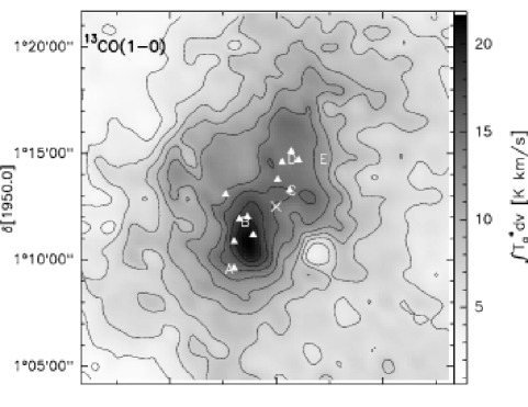
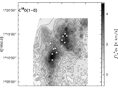
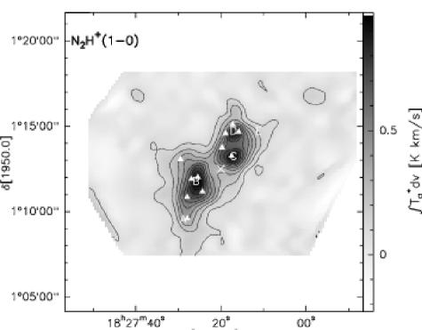
Figure 1: Maps of the ¹³CO, C¹⁸O and N₂H⁺ integrated intensity in the velocity interval 4.0 to 12.0 km s^-1. In the ¹³CO map the value of the first contour is 1.5 K km s^-1and the contour interval is 1.0 K km s^-1. In the C¹⁸O and N₂H⁺ maps the value of the first contour and the contour interval are both 0.4 K km s^-1. The cross marks the reference position (see Table 1) and the filled triangles represent the positions of the submillimeter continuum sources. The letters mark the positions of the main N₂H⁺ cores as defined in TSOO. The “spur” is also visible, an extended, lower surface brightness narrow region, stretching from the NW to SE clumps and continuing beyond these (see also Fig. 2).

The paper is organized as follows: in Sect. 2 and 3 we describe the new observations, the morphology of the Serpens cloud in the observed tracers and derive the physical conditions of the molecular gas; in Sect. 4 we discuss the cloud kinematical and fragmentation properties; finally, in Sect. 5 we summarize the main results of this study, and we discuss the implications for cluster formation and evolution theories.

2 Observations

Table 1: Molecular transitions observed and their rest frequencies. The third column lists the size of the map centered about the position $\alpha=18^{\rm h}27^{\rm m}20^{\rm s}$ and $\delta=1^{\circ}12^{\prime}30^{\prime\prime}$ (B1950.0)

Line	Frequency [GHz]	Map size [arcmin]
CS(2–1)	97.980968	$13\times 10$
C34S(2–1)	96.412982	$5\times 5$
N2H+(123–012)	93.1734796	$13\times 10$
13CO(1–0)	110.201353	$16\times 16$
C18O(1–0)	109.782182	$12\times 14$

The single dish observations of the Serpens cloud core were carried out in March, October and November 1999 with the 13.7-m telescope of the FCRAO located in New Salem (U.S.A.), using the new SEQUOIA 32 element focal plane array, although for the present observations only 16 pixels were actually used. The observed lines and their rest frequencies are listed in Table 1. The maps were centered about the position $\alpha=18^{\rm h}27^{\rm m}20^{\rm s}$ and $\delta=1^{\circ}12^{\prime}30^{\prime\prime}$ (B1950.0), and the FWHM of the FCRAO telescope varied from about $46^{\prime\prime}$ to about $53^{\prime\prime}$. The front-end receivers employed low noise InP MMIC-based amplifiers resulting in a mean receiver temperature of 70 K (SSB) and system temperatures typically in the range $160-250$ K. Our spectrometer was an autocorrelator with 24 KHz (0.077 km s^-1) spectral resolution and 20 MHz bandwidth.

The integration times used for the single-scan were typically 5 to 25 minutes in frequency switching mode, using a frequency throw of 8 MHz. The maps were carried out using 1-beam sampling and the sizes of the covered regions in the different lines are also listed in Table 1. The main beam efficiency used to convert the antenna temperature, $T_{\rm A}^{*}$, to main beam brightness temperature is $\eta_{\rm mb}=0.55$. The final achieved sensitivities in the $T_{\rm A}^{*}$ scale varied from about 0.05 K for C³⁴S to about 0.19 K for ¹³CO.

3 Results

3.1 Morphology of the Serpens region

3.1.1 ¹³CO(1–0) and C¹⁸O(1–0)

We performed wide-field imaging of the ¹³CO and C¹⁸O(1–0) emission towards the Serpens region to understand the relation of the global distribution of the molecular gas with the denser gas in the cloud cores. The optically thicker ¹³CO(1–0) line emission tends to pick up the more diffuse ambient gas, whereas the thinner transition of C¹⁸O(1–0) shows the distribution of the gas inside the Serpens cloud.

The ¹³CO(1–0), C¹⁸O(1–0) and N₂H⁺(1–0) emission integrated over the velocity interval 4.0 to 12.0 km s^-1, shown in Fig. 1, trace the distribution of the column density in the Serpens cloud (see also Sect.3.4.1). The ¹³CO emission is extended and encompasses both the NW and SE clusters of submillimeter continuum sources, with a peak of emission near the position of SMM4. We clearly detect ¹³CO(1–0) at the position of SMM1, where the BIMA observations of McMullin et al. (mcm00 (2000)) did not detect any emission. Compared to the C¹⁸O(1–0) map of McMullin et al. (mcm00 (2000)) our C¹⁸O integrated intensity map better shows the clear demarcation between the NW and SE sub-clusters, which are also separated in velocity (see Sect. 3.3 and TSOO).

The NW clump is clearly surrounding all continuum sources: S68N (McMullin et al. mcm94 (1994)) and SMM1 in particular (also seen at the position of the N₂H⁺ core C) are very close to two C¹⁸O emission peaks. The SE cluster of submillimeter continuum sources lies essentially in the region between the two C¹⁸O peaks, and is aligned with the C¹⁸O lower surface brightness region extending to the NE. On the other hand, sources SMM2 and SMM11 are embedded in the SE gas clump, and the emission is elongated in the NS direction along the “spur”, an extended, lower surface brightness narrow region, stretching from the NW to SE clumps and continuing beyond these, observed by TSOO. As observed by McMullin et al. (mcm00 (2000)), in the case of the C¹⁸O emission there is a lack of correspondence with the submillimeter peaks, especially in the SE sub-clump. However, the C¹⁸O and submillimeter dust continuum emission both trace the large-scale distribution of column density, as shown in Fig. 2. A similar structure to C¹⁸O can be seen in N₂H⁺ (TSOO), although the peaks of emission show a different position in the SE clump.

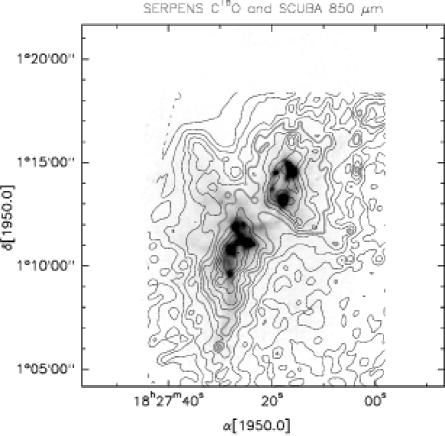
Figure 2: Overlay of SCUBA 850 $\mu$m gray-scale image (kindly provided by C.J. Davis, Davis et al. dav99 (1999)) and C¹⁸O(1–0) integrated emission (contour levels as in Fig. 1). The thicker grey contour corresponds to 50% of the maximum.

Fig. 2 shows that the Spur emission has a striking correspondence with the 850 $\mu$m continuum emission of Davis et al. (dav99 (1999)) extending southward from SMM11. Another dust lane is extending roughly NE from SMM3 and coincides quite well with a “bulge” of higher velocity gas visible in both the ¹³CO and C¹⁸O centroid velocity maps (Fig. 8). Here, as suggested by Davis et al. (dav99 (1999)), the high-velocity gas and dust continuum emission are maybe showing the action of a wind powered by the SMM 2/3/4 group.

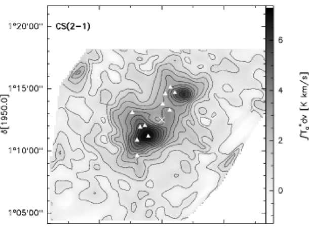
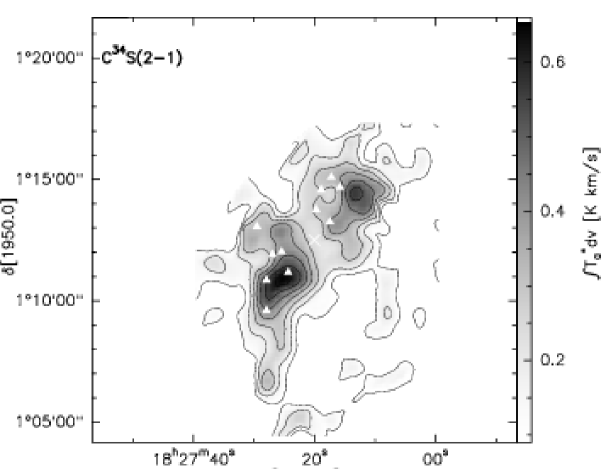
Figure 3: Maps of the CS and C³⁴S integrated intensity in the velocity interval 2.0 to 13.0 km s^-1 (CS) and 5.0 to 11.0 km s^-1 (C³⁴S). In the CS map the value of the first contour is 0.24 K km s^-1and the contour interval is 0.6 K km s^-1. In the C³⁴S map the value of the first contour and the contour interval are both 0.09 K km s^-1.

3.1.2 CS(2–1) and C³⁴S(2–1)

To determine the distribution of the denser gas in Serpens we obtained integrated intensity maps of the CS and C³⁴S(2–1) emission (see also Sect.3.4). The maps are presented in Fig. 3, where CS and C³⁴S(2–1) show several condensations and the two main clumps, NW and SE. A detailed comparison with the N₂H⁺ and C¹⁸O unveils several important differences. TSOO showed that the N₂H⁺ map follows the spatial distribution of the submillimeter sources in both the NW and SE sub-clumps much more closely than the other molecular tracers such as C³²S and CH₃OH. This is confirmed by our new single dish C³²S and C³⁴S maps, showing that the CS distribution resembles much more closely that of other shock tracers, such as H₂CO (McMullin et al. mcm00 (2000)), in agreement with what found by TSOO.

3.2 Line profiles

TSOO mapped the NW and SE clumps of the Serpens region in the N₂H⁺(1–0) transition and found four main cores of emission, A, B spatially associated with the SMM3/4 sources in the SE clump, and C, D associated with SMM1/S68N in the NW region. As mentioned earlier, they also identified an extended, lower surface brightness Spur, stretching from the NW to SE clumps. Spectra of N₂H⁺ and also of CS, C³⁴S and C¹⁸O at the emission peaks of these regions are presented in Figs. 4 to 6. Our maps of the Serpens region obtained using CS, C³⁴S and C¹⁸O complement the N₂H⁺ observations of TSOO and show some new features. In particular, the Spur is detected in all molecular tracers observed by us and its emission only covers a narrow ($\simeq 0.4-0.5$ km s^-1) velocity range. The N₂H⁺(1–0) emission is mostly optically thin, except at the emission peaks in the NW clump where $\tau({\rm N_{2}H^{+}})\mathrel{\mathchoice{\vbox{\offinterlineskip\halign{\hfil$\displaystyle#$\hfil\cr<\cr\sim\cr}}}{\vbox{\offinterlineskip\halign{\hfil$\textstyle#$\hfil\cr<\cr\sim\cr}}}{\vbox{\offinterlineskip\halign{\hfil$\scriptstyle#$\hfil\cr<\cr\sim\cr}}}{\vbox{\offinterlineskip\halign{\hfil$\scriptscriptstyle#$\hfil\cr<\cr\sim\cr}}}}1$.

3.2.1 ¹³CO(1–0) and C¹⁸O(1–0)

The ¹³CO spectra in the NW clump appear to be self-absorbed (see Fig. 5), as the dip is at about the same velocity as that of the CS spectra ($\simeq 8.6$ km s^-1) and is aligned with the C³⁴S peak. The C¹⁸O spectra appear to have a Gaussian profile in the NW clump and are mostly optically thin. In this clump the peak of the C¹⁸O line is generally well aligned with those of C³⁴S and N₂H⁺ and traces the dip of the ¹³CO and CS spectra (see Figs. 5 and 6).

In the SE clump the line shape of ¹³CO tends to be non-Gaussian, especially at offsets $\delta<-100^{\prime\prime}$ and $\alpha>20^{\prime\prime}$ from the map center. As for the N₂H⁺ line shape, the C¹⁸O non-Gaussian profile is due to the presence in the beam of several velocity components (cores “A”, “B” and the “Spur” of TSOO), as shown in Fig. 4 where the two N₂H⁺ peaks are nicely aligned with those of C¹⁸O. It is interesting to note that the ratio of ¹³CO to C¹⁸O emission is lower in the Spur than at the other positions. For example at the position and velocity of core A, $(133,-177)$ and $V_{\rm LSR}=7.15$ km s^-1, the ¹³CO to C¹⁸O intensity ratio is about 3, whereas at the velocity of the Spur this ratio decreases to about 2.

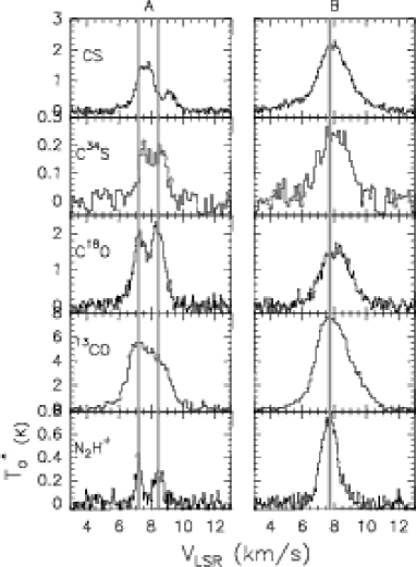
Figure 4: Line spectra at position A(133,-177) and B(88,-44) in the SE sub-cluster. From top to bottom: CS(2–1), C³⁴S(2–1), C¹⁸O(1–0), ¹³CO(1–0), and N₂H⁺(1₀₁–0₁₂). The vertical lines are drawn at the peak velocities of the N₂H⁺ Gaussian fits. The highest velocity N₂H⁺ component corresponds to the emission from the “Spur”.

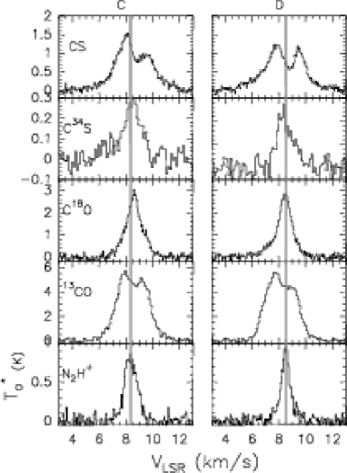
Figure 5: Same as Fig. 4 for positions C(-44,44) (i.e., SMM1) and D(-44,133) (or S68N) in the NW sub-cluster

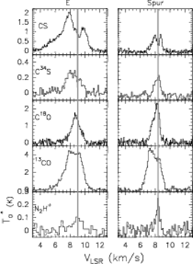
Figure 6: Same as Fig. 4 for positions E(-133,133) (or S68NW) and at one position in the Spur, (133,-310)

3.2.2 CS(2–1) and C³⁴S(2–1)

Most of CS spectra in the NW clump (see Fig. 5) are self-absorbed and are optically thick, as confirmed by the presence of the C³⁴S emission peaks at the dip of the CS spectra (see also Williams and Myers WM99 (1999)). The differences in the profiles between the two isotopomers are mainly due to their different optical depths: the C³⁴S lines are optically thin and single-peaked whereas the CS spectra generally present two peaks. The asymmetries in the self-absorbed CS spectra have been interpreted by Williams and Myers (WM99 (1999)) as the signpost of a large-scale contraction of the gas around the clusters. The blue asymmetric line profile of CS is visible in both the NW and SE clumps, and by comparing CS and C³⁴S we will show later that in these regions the centroid velocity of the optically thicker isotopomer is lower (bluer) than its rarer and optically thin counterpart.

The CS spectra show line wings due to outflows from several cluster sources, such as S68N and SMM1 in the NW clump, and SMM3 and SMM4 in the SE clump. The CS spectra in the Spur are self-absorbed, as shown in Fig. 6, and both the N₂H⁺ and C¹⁸O emission peaks are aligned with the dip of the CS spectra.

3.3 Kinematics of the Serpens region

The analysis of the gas kinematics in the Serpens region is complicated by the presence of several velocity fields that may include infall, rotation, turbulence and outflow motions. In particular, the presence of several known outflows may render the unambiguous detection of either rotation or infall very difficult. In this work we did not attempt to detect infall motions around some of the specific submillimeter sources, but we were instead interested in the global motions of the cloud and within the cloud. The molecular tracers used also reflect this goal: their excitation conditions make ¹³CO and C¹⁸O(1–0) less prone to contamination by outflows. Likewise, the two optically thin tracers C³⁴S(2–1) and N₂H⁺(1–0) are not affected by the presence of outflows. However, the CS(2–1) emission is known to be contaminated in the presence of strong outflows (see TSOO and refrences therein) and indeed we detect line wings in the CS lines (see Sect. 3.2.2).

We present the velocity information in four different graphical forms designed to emphasize different kinematical properties of the gas: (i) line core, red and blue wing maps to show large-scale velocity structures; (ii) centroid velocity maps, to show small velocity trends of the cloud bulk emission; (iii) normalized centroid velocity difference between an optically thick and a thin tracer, to show systematic differences such as infall motions; (iv) line width maps, to show the velocity dispersion accross the region for the various tracers.

3.3.1 Line core and line wings maps

To determine the velocity distribution of the ambient gas in Serpens we made integrated intensity maps of the blueshifted ($5.0-7.3$ km s^-1), line core ($7.3-8.4$ km s^-1) and redshifted ($8.4-12.4$ km s^-1) emission of ¹³CO and C¹⁸O(1–0). The maps are shown in Fig. 7 where the ¹³CO and C¹⁸O  emission is clearly separated and occupies mainly the half-plane to the East in the blueshifted channel, whereas the emission is mostly concentrated in the half-plane to the West in the redshifted channel (see also Fig. 8). In particular, ¹³CO shows a very different distribution from that of CO(1–0) (McMullin et al. mcm94 (1994)) and (2–1) (Davis et al. dav99 (1999)). In fact, while the CO emission is affected by the high-velocity gas radiated from the submillimeter sources, ¹³CO is less affected by molecular ouflows and thus can better show the kinematics of the large-scale gas. In the central velocity map of C¹⁸O the Spur is clearly visible as a gas filament extending southward from the SE cluster of submillimeter sources.

The maps in Fig. 7 show emission from the SE and NW sub-clusters at all velocities, although the C³⁴S emission is weak in the $5.0-7.3$ km s^-1velocity interval and is mostly concentrated in the SE clump. We also note that the C¹⁸O(1–0) emission from the NW clump is concentrated in the line core and especially in the redshifted channel. The morphology shown by the channel maps of the two CO isotopomers and of the density sensitive tracers is clearly different. The ¹³CO and C¹⁸O(1–0) line emission show a velocity gradient roughly E to W whereas CS(2–1) is tracing the embedded denser cloud cores and the EW velocity gradient is much less evident.

Moreover, they show other isolated cores of emission, such as S68N, visible in the CS central velocity map. This core has a weak N₂H⁺ counterpart shown in the N₂H⁺ channel map of TSOO at a velocity of about 8.2 km s^-1. Another emission peak at the position of SMM1 is visible in both the CS and C³⁴S 8.4–12.4 km s^-1channel maps; in C³⁴S this emission peak is also visible in the other velocity channels. The Spur is also visible in the central velocity map. Finally, in the CS 8.4–12.4 km s^-1channel map the SE sub-cluster appears to be composed of two separate cores, one at the position of SMM4 and the other slightly north of the SMM 3/6 group.

The central velocity ¹³CO map shows an emission peak at the position of SMM4 and of the CS peak. Another peak is visible sligthly NW of SMM3; the N₂H⁺ core B is positioned between these two emission peaks. In the 5.0-7.3 km s^-1channel map a sharp peak of ¹³CO emission is visible South of SMM4, which is also the region of C¹⁸O emission, although the peaks are not coincident. A secondary peak of C¹⁸O emission can be found in the NE region of this velocity channel that is coincident with enhanced ¹³CO emission. There are clearly two velocity components overlapping at this position, as shown by the C¹⁸O and ¹³CO spectra.

3.3.2 Large-scale velocity gradient

The velocity gradient of an interstellar gas cloud can be determined by using all or most of the data in a map at once, by least-squares fitting maps of line-center velocity for the direction and magnitude of the best-fit velocity gradient (see Goodman et al. good93 (1993) and references therein).

A cloud undergoing solid-body rotation would exhibit a linear gradient, ${\rm d}V/{\rm d}r$, across the face of a map, perpendicular to the rotation axis. Thus, following Goodman et al. (good93 (1993)) we fit the function

$$\mbox{$V_{\rm LSR}$}=V_{o}+a\Delta\alpha+b\Delta\delta$$ (1)

to the peak velocity of a Gaussian fit to the emission profile of several molecular tracers. Here, $\Delta\alpha$ and $\Delta\delta$ represent offsets in right ascension and declination, expressed in radians, $a$ and $b$ are the projections of the gradient per radian on the $\alpha$ and $\delta$ axes, respectively, and $V_{o}$ is the LSR systemic velocity of the cloud. The magnitude of the velocity gradient, in a cloud at distance $d$, is thus given by

$$\frac{{\rm d}V}{{\rm d}r}=\frac{(a^{2}+b^{2})^{1/2}}{d}$$ (2)

and its direction (measured east of north) is

$$\theta_{\rm v}=\tan^{-1}\frac{a}{b}$$ (3)

In order to carry out a least-squares fit to Eq.(1) we have computed the following error function

$$\chi^{2}=\sum_{i,j}{}\left[\frac{\mbox{$V_{\rm LSR}$}(i,j)-V_{o}-a\Delta\alpha_{i}-b\Delta\delta_{j}}{\sigma_{v}(i,j)}\right]^{2}$$ (4)

where $\mbox{$V_{\rm LSR}$}(i,j)$ is the velocity of the Gaussian fit to the spectrum at position $(\Delta\alpha_{i},\Delta\delta_{j})$ in the map, and $\sigma_{v}(i,j)$ is the uncertainty in $V_{\rm LSR}$ determined by the fit, given by (see Goodman et al. good93 (1993) and references therein):

$$\sigma_{v}=1.15\left(\frac{\sigma_{T}}{T}\right)(\delta_{v}\Delta V)^{1/2}$$ (5)

where $T$ is the peak of a Gaussian fit to the line profile, $\sigma_{T}$ is the RMS noise in the spectrum, $\delta_{v}$ is the velocity resolution of the spectrum and $\Delta V$ is the FWHM line width. Only those points for which SNR$=T/\sigma_{T}>3$ were used in Eq.(4).

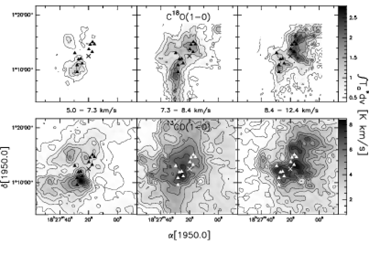
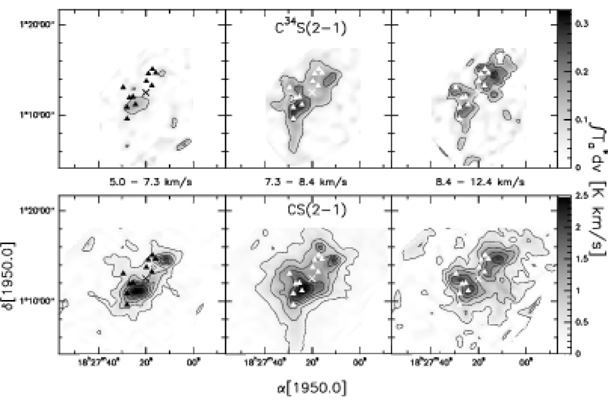
Figure 7: From top to bottom: line core and line wings integrated intensity maps for C¹⁸O, ¹³CO, C³⁴S, and C³²S.

To find the minimum of the function expressed by Eq.(4) we have used the downhill simplex method, using “AMOEBA” of Press et al. (nr92 (1992)) as the basic multidimensional minimization routine. The results are listed in Table 2 for the various molecular tracers. Two comments are in order: (i) N₂H⁺ and C³⁴S trace the denser gas in the cores and are thus less suited to calculate the large-scale velocity gradient; (ii) ¹³CO is mostly optically thick with a non-Gaussian line profile and it is also not reliable. For these reasons we choose C¹⁸O as the best available tracer to us of the velocity gradient in the Serpens cloud. Despite the aforementioned caveats, the direction of the velocity gradient is not significantly different from one tracer to another and confirms our early assumption in Sect. 3.3.1 that the Serpens cloud exhibits a velocity gradient roughly E to W.

Table 2: Results of velocity gradient fitting.

Line	$V_{o}$	${\rm d}V/{\rm d}r$	$\theta_{v}$
	[km s-1]	[km s-1 pc-1]	[deg E of N]
C18O(1–0)	8.31	1.25	-88.9
13CO(1–0)	8.03	0.75	-70.8
C34S(2–1)	8.42	2.03	-78.9
N2H+(123–012)	8.34	0.54	-72.4

3.3.3 Centroid velocity maps

The centroid velocity of a line is that velocity at which the integrated intensity is equal on either side of the line profile, and we compute it as in Narayanan et al. (nar98 (1998)). Centroid velocity maps are usually a good indicator of global velocity structures, such as rotational motions, and we use them here as further evidence of the large-scale velocity gradient found in the previous section.

In Fig. 8 we present the centroid velocity maps of the ¹³CO and C¹⁸O lines. To minimize the potential contamination of the kinematics of the cloud by the outflow velocity fields, the centroid velocities were computed over line core intervals ($6.0-10.5$ km s^-1) which must also be wide enough to encompass the line core emission in both the NW and SE sub-clumps. Both maps show an increasing gradient in centroid velocity from roughly E to W, as expected.

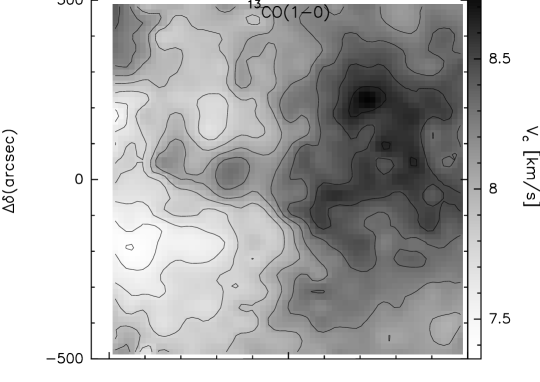
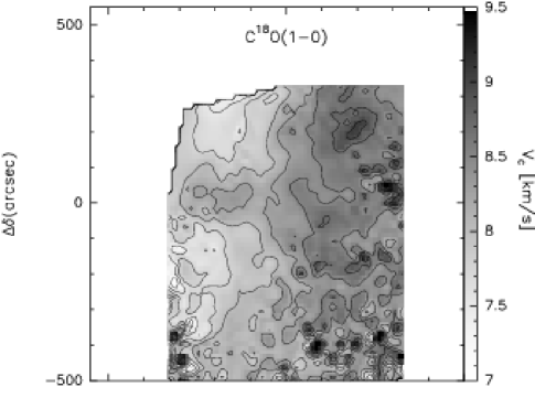
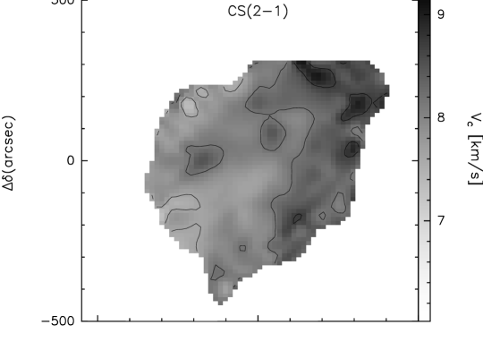
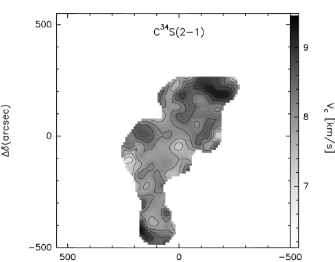
Figure 8: Centroid velocity maps for: ¹³CO, C¹⁸O, C³²S, and C³⁴S (from top to bottom). The centroid velocities are obtained over the velocity interval corresponding to the line core (6 to 10.5 km s^-1). Only the observed points where the integrated intensity is greater than three times its corresponding RMS uncertainty are used in calculating the centroid velocity. The offsets are measured with respect to the center position listed in Table 1.

The maps shown in Fig. 8 also show a velocity “bulge” extending from about the map center towards the E, which may be caused by one of the redshifted CO(1–0) outflow lobes found by Narayanan et al. (nmwb01 (2002)), despite our centroid velocities are calculated using only line core emission. Even if some contamination of the centroid velocity maps by the outflows may still be present, the velocity gradient observed in the maps of Fig. 8 is extended to the whole Serpens cloud and is unlikely that the ¹³CO and C¹⁸O centroid velocities are seriously affected by the outflows. We can also exclude that the observed velocity gradient is due to separate clumps with different systemic velocities, as the differences in the lines $V_{\rm LSR}$ are less or comparable with the line FWHM of C¹⁸O and show a smooth change from E to W. As will be further discussed in Sect. 4.1, we conclude that the observed velocity gradient may indeed be caused by a global rotation of the Serpens molecular cloud whose rotation axis is roughly aligned in the SN direction.

In Fig. 8 we also present the centroid velocity maps of the CS and C³⁴S(2–1) transitions. The CS map shows essentially a plateau in the region where most of the CS(2–1) emission is detected. Our spatial resolution is not good enough to distinguish any particular feature around specific submillimeter sources. However, we note once again the small bulge of redshifted emission E of the map center.

3.3.4 Normalized velocity difference maps and infall speeds

A diagnostics which is often used to disentangle the large-scale kinematics of molecular cloud cores is based on the normalized centroid velocity difference (see Mardones et al. mard97 (1997)). The normalized centroid velocity difference $\delta V_{\rm c}$ is a non-dimensional parameter defined as:

$$\delta V_{\rm c}=\frac{V_{\rm c}({\rm CS})-V_{\rm c}({\rm C^{34}S})}{\Delta V({\rm C^{34}S})}$$ (6)

and is very useful to quantify the observed line asymmetries in the optically thick CS(2–1) line. Alternatively, one can use N₂H⁺(1–0) to replace C³⁴S as the optically thin tracer in Eq. (6). A blue asymmetry ($\delta V_{\rm c}\leq 0$) can be interpreted as an indication of infall motion (Myers et al. Mea96 (1996); Mardones et al. mard97 (1997)).

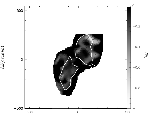
Figure 9: Normalized centroid velocity difference map of CS and C³⁴S. The centroid velocities were calculated over the velocity interval 5.5 to 10.5 km s^-1. To better show the contrast between the regions where $\delta V_{\rm c}<0$ and those where $\delta V_{\rm c}>0$ the upper limit for this map has been set equal to 0. The thick white line represents the contour for the 50% of the peak of the H₂ column density.

In Fig. 9 the map of $\delta V_{\rm c}$ as defined in Eq. (6) is shown. We decided to use CS as the optically thick tracer and C³⁴S, rather than N₂H⁺, as the optically thin tracer to ensure that both species have homogeneous chemical properties. We can see that there are two regions of the map where the negative values of $\delta V_{\rm c}$ are more concentrated, which are approximately coincident with the SE and NW sub-clumps. This indicates that there is molecular gas around the SE and NW sub-clusters which is still undergoing an infalling motion.

Typical infall speeds at different positions in the SE and NW clumps can be calculated by using the simple two layer model of Myers et al. (Mea96 (1996)), which gives:

$$V_{\rm in}\simeq\frac{\sigma_{\rm v}}{V_{\rm red}-V_{\rm blue}}\log\left(\frac{1+eT_{\rm BD}/T_{\rm D}}{1+eT_{\rm RD}/T_{\rm D}}\right)$$ (7)

where $T_{\rm D}$ is the brightness temperature of the dip in the CS line shape, $T_{\rm BD}$ is the height of the blue peak above the dip, and $T_{\rm RD}$ is the height of the red peak above the dip. The velocity dispersion $\sigma_{\rm v}$ can be obtained from the FWHM of an optically thin line, such as N₂H⁺, thus $\sigma_{\rm v}=\Delta V_{\rm N_{2}H^{+}}/\sqrt{8\log 2}$. The results are shown in Table 3, where the first two positions refer to the SE clump, and the next three correspond to the NW clump. In the SE clump (including position B, not shown in Table 3) the CS line profiles are more symmetric, implying a lower infall speed, except near position A where $V_{\rm in}>0.2$ km s^-1. This suggests different states in the core contraction process, as also shown by Fig. 9.

Table 3: Line velocity dispersion of N₂H⁺ (second column), non-thermal velocity dispersion (third column) and infall speeds (fourth column) towards the SE and NW sub-clumps ($\sigma=\Delta V/\sqrt{8\log 2}$).

Position	$\sigma_{\rm v}$	$\sigma_{\rm NT}$	$V_{\rm in}$
	[km s-1]	[km s-1]	[km s-1]
A	0.33	0.32	0.26
(88,-177)	0.35	0.34	0.21
C	0.49	0.48	0.35
D	0.35	0.34	0.09
E	0.62	0.58	0.44

A similar difference clearly exists in the NW sub-clump, where positions C and E show substantially different infall speed compared to position D. This difference has also been observed by Williams & Myers (WM99 (1999)), and our results confirm their conclusion about the presence of supersonic ($V_{\rm in}>\sigma_{\rm th}[{\rm H_{2}}]=0.27$ km s^-1at $T=20$ K) inward motions in the NW sub-clump, and indicate near-supersonic contraction in the SE sub-clump.

For these same positions we can quantify the turbulent motion by comparing the N₂H⁺ line FWHM with that expected for gas having equal thermal and non-thermal motions (Mardones et al. mard97 (1997), Lee et al. L99 (1999)):

$$\Delta V_{\circ}=\left[8\log 2\,kT\left(\frac{1}{m_{\rm N_{2}H^{+}}}+\frac{1}{m_{\rm av}}\right)\right]^{1/2}$$ (8)

where T is the gas kinetic temperature, $k$ is the Boltzmann constant, $m_{\rm N_{2}H^{+}}$ is the molecular weight of N₂H⁺ (29 amu), and $m_{\rm av}$ is the gas mean molecular weight (2.3 amu). For gas with $T=20$ K, we find that $\Delta V_{\rm N_{2}H^{+}}>\Delta V_{\circ}=0.66$ km s^-1, thus having greater non-thermal than thermal motions (see Table 3). This result is consistent with the prevalence of turbulent infall motions in a sample of cores with embedded YSOs found by Mardones et al. (mard97 (1997)), whereas Lee et al. (L99 (1999)) found that most starless infall candidates are in a state of thermal infall. Incidentally, we note that also the starless core at position E has a greater turbulent rather than thermal motion.

The aim of this paper is not to calculate the mass infall rate for every cloud core, as our spatial resolution is not high enough. However, for consistency we did calculate the kinematic mass infall rate, $({\rm d}M/{\rm d}t)_{\rm kin}=4\pi R_{\rm in}^{2}\left<m_{\rm av}n_{\rm H_{2}}\right>V_{\rm in}$, toward position E. The infall radius was taken from Williams & Myers (WM99 (1999)), $R_{\rm in}=6200$ AU, $V_{\rm in}=0.44$ km s^-1 from Table 3, and $\left<m_{\rm av}n_{\rm H_{2}}\right>$ was obtained by taking the average of all mass estimates in Table 4 (except for the values obtained from the statistical equilibrium method, see Sect. 3.4.2) and dividing by the total volume of the NW clump. Thus, we obtain $({\rm d}M/{\rm d}t)_{\rm kin}\simeq 5\,10^{-5}$ M_⊙yr^-1. This value can be compared with the gravitational mass accretion rate of $({\rm d}M/{\rm d}t)_{\rm gr}=0.975a^{3}/G$ (Shu shu77 (1977)), where $a$ is the velocity dispersion of the molecule of mean mass $m_{\rm av}$, $a^{2}=kT/m_{\rm av}+\sigma_{\rm NT}^{2}$. Using $T=20$ K and $\sigma_{\rm NT}$ from Table 3, we find $({\rm d}M/{\rm d}t)_{\rm gr}\simeq 5.9\,10^{-5}$ M_⊙yr^-1. The agreement of these two rates indicates that the derived inward motion at position E is consistent with gravitational infall.

3.3.5 Line width maps

Another useful diagnostic tool is to plot a measure of the width of the line profile. Given the deviation from a Gaussian line profile presented by some of the observed molecular tracers, in Fig. 10 we show the maps of the $2^{nd}$ moment of the data.

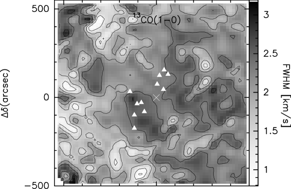
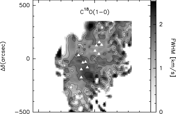
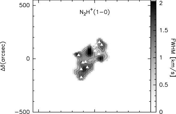
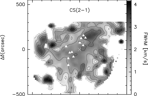
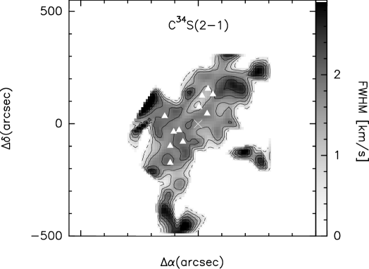
Figure 10: Maps of the $2^{nd}$ moment of the data (line width). From top to bottom: ¹³CO, C¹⁸O, N₂H⁺, C³²S, C³⁴S. Data with SNR$<5\sigma$ have been masked out. The N₂H⁺ map shows the $2^{nd}$ moment of the first hyperfine component.

The map of the ¹³CO line width in Fig. 10 clearly shows that the FWHM in the SE clump is enhanced compared to the rest of the ambient cloud. Although to a lesser extent, this is also seen in the NW clump. The C¹⁸O line widths are also larger in the SE clump, which is also an effect of the presence of the two velocity components (clumps A, B and the Spur) in this part of the cloud. A two-component Gaussian fit in the SE region shows that most of the contribution to the line width of C¹⁸O(1–0) comes from the lowest velocity component, although the peak of the line-FWHM is shifted relatively to the nominal positions of the clumps A and B.

Likewise, the N₂H⁺(1–0) map shows an enhacement of the line width in the SE clump, whereas this is less evident in the NW clump, also due to the limited extension of the map in that region. The CS(2–1) and C³⁴S(2–1) maps of the $2^{nd}$ moment of the data shown in Fig. 10 show some enhacement of the line width at the positions of the submillimeter sources, but the most noticeable feature is the much larger line width at the position of the S68NW starless core described by Williams & Myers (WM99 (1999)).

3.4 Physical parameters

In this section we derive the physical parameters of the molecular gas, using various tracers and approximations. We first derive estimates of the gas excitation and column densities using a simplified LTE approximation, then we derive particle densities from the C³⁴S line intensities using an LVG approximation combining our data with the C³⁴S(5-4) observations of McMullin et al. (mcm94 (1994)). Finally, we provide various estimates of the masses of the entire cloud and of the various clumps identified by TSOO.

3.4.1 Excitation and column densities

The C¹⁸O emission can be used to trace the column density of the Serpens cloud. To derive values for the column density we first estimated the excitation temperature throughout the entire region, based on the ¹³CO line temperatures at a velocity of 8.58 km s^-1. We also estimated the C¹⁸O optical depths using the ¹³CO to C¹⁸O line ratio and a relative abundance $X$[¹³CO]/$X$[C¹⁸O]$=12$. We then used both $T_{\rm ex}$ and $\tau$(C¹⁸O) to calculate the column density of a $J\rightarrow J-1$ rotational transition according to the following formula (Lis & Goldsmith lg91 (1991)):

$$N_{\rm tot}=\frac{4.0\times 10^{12}}{J^{2}\mu^{2}\,B}Z\exp\left(\frac{E_{\rm J}}{T_{\rm ex}}\right)\frac{1}{\eta_{\rm mb}}\frac{\tau}{1-e^{-\tau}}\int\,T_{\rm A}^{\star}\,{\rm d}v$$ (9)

where $B$ denotes the rotational constant, $E_{\rm J}$ is the upper state energy, $\mu$ is the dipole moment and we use the escape probability $\tau/[1-\exp(-\tau)]$ to account for first order optical depth effects. We also assume a unity beam-filling factor. The excitation temperature is obtained by inverting the equation of transport:

$$\mbox{$T_{\rm mb}$}=[J_{\nu}(\mbox{$T_{\rm ex}$})-J_{\nu}(\mbox{$T_{\rm bg}$})]\,[1-\exp(-\tau)]$$ (10)

where $T_{\rm ex}$ and $\tau$ are calculated at a specific velocity and $\tau$ is evaluated as described above. Moreover, for $kT_{\rm ex}>>hB$ the partition function of a linear molecule is given by

$$Z=\frac{kT_{\rm ex}}{hB}$$ (11)

where $h$ is the Planck constant. The distribution of $N_{\rm tot}$(H₂) calculated using C¹⁸O data is shown in Fig. 11 and corresponds very well to the map of the C¹⁸O integrated emission of Fig. 1.

The CS and C³⁴S data can be used to derive the gas total column density following the method described above for ¹³CO and C¹⁸O. C³⁴S is in fact optically thin and can thus be successfully used to trace the column density of the gas if its relative abundance can be determined. We derived the C³⁴S abundance using the LVG approximation to model the measured line intensities, as described later in this section. Therefore, we can use C¹⁸O and C³⁴S to compare the spatial distributions of the column density and excitation temperature at two velocities characterizing the NW (8.58 km s^-1) and SE (7.3 km s^-1) sub-clumps. We find that CS and C¹⁸O show a different behaviour: in fact, the C¹⁸O maps present a spatial offset between the peaks of $T_{\rm ex}$ and those of the gas column density distributions (see Fig. 11). At the velocity of the NW sub-clump the C¹⁸O column density map shows a clump that surrounds the NW group of submillimeter sources, whereas the map of $T_{\rm ex}$ shows a smooth plateau at the same position. At the velocity characterizing the SE sub-clump these differences are less extreme: a broad peak of column density surrounds sources SMM2/4/11, whereas the $T_{\rm ex}$ map peaks between SMM4 and SMM3/6. In both the NW and SE sub-clumps the distribution of the column density (see Fig. 11) follows quite closely the map of the C¹⁸O integrated emission shown in the bottom panel of Fig. 1, suggesting that the emission peaks are column density maxima and are not due to peaks in the excitation of the molecular gas.

The CS and C³⁴S transitions can also be used to determine the spatial distribution of $T_{\rm ex}$(C³²S) and the column density. The map of $T_{\rm ex}$(C³²S) has a broad peak including the SMM 3/4/6/8 group. The gas traced by CS, however, is characterized by spatial distributions of $T_{\rm ex}$ and column density that are much more similar (see Fig. 12). In the NW sub-cluster the column density map shows a peak at the position of S68NW, while $T_{\rm ex}$ has a maximum slightly NW of the S68NW position. At the velocity characterizing the SE sub-cluster, the $T_{\rm ex}$ and column density maps both have a peak very close to the position of SMM4 and show little differences otherwise. Therefore, there is a tendency of the gas column density to have a different spatial distribution from that of $T_{\rm ex}$ in the NW sub-cluster, and this difference is much more evident in C¹⁸O.

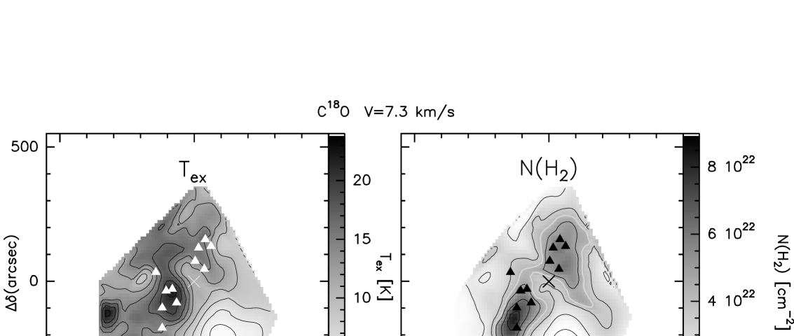
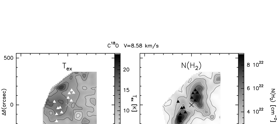
Figure 11: Maps of $T_{\rm ex}$ and of H₂ column density using C¹⁸O and a velocity of 7.3 km s^-1(top) and 8.58 km s^-1(bottom), characteristic of the SE and NW clumps, respectively.

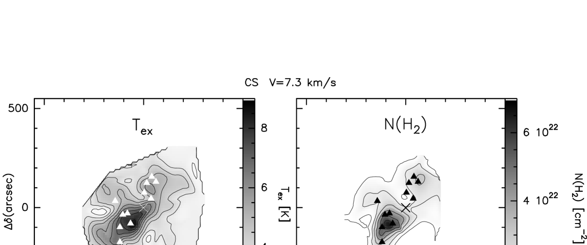
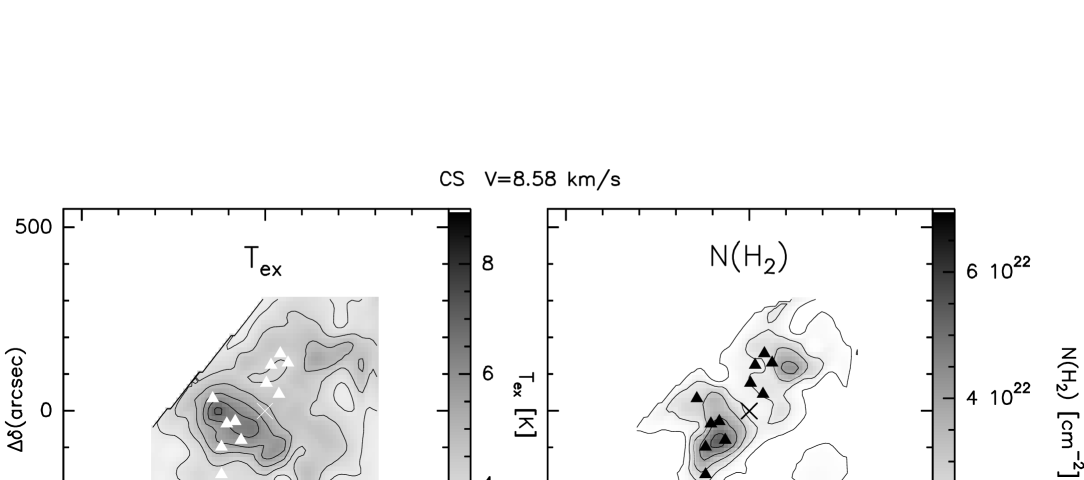
Figure 12: Maps of $T_{\rm ex}$ and of H₂ column density using CS and a velocity of 7.3 km s^-1(top) and 8.58 km s^-1(bottom), characteristic of the SE and NW clumps, respectively.

3.4.2 Density estimates

The physical number densities towards the densest condensations can be derived using density tracers such as the optically thin C³⁴S transitions. Because we observed the $J=2-1$ line only, we also used the C³⁴S(2–1) and (5–4) observations towards SMM1 of McMullin et al. (mcm94 (1994)). By using the $J=2-1$ measurements taken with the FCRAO and NRAO telescopes we were able to estimate the deconvolved angular diameter of the source $\theta_{\rm s}\simeq 70^{\prime\prime}$. Assuming a gas temperature of 35 K towards SMM1 and a velocity gradient of about 21 km s^-1 pc^-1, we then used the LVG approximation to model the measured line intensities, obtaining a number density $\mbox{$n_{\rm H_{2}}$}\simeq 5.6\times 10^{5}$ cm^-3 and a relative abundance $X$[C³⁴S]/$X$[H₂]$=4\times 10^{-11}$, which are consistent with the values obtained by McMullin et al. (mcm00 (2000)). There are no C³⁴S(5–4) observations towards the SE sub-clump. However, an estimate of the physical conditions at the SMM4 position can be derived by using the LVG model parameters obtained for SMM1, and changing one parameter only, e.g. the density, to fit the C³⁴S(2–1) line intensity. By doing this we derive $\mbox{$n_{\rm H_{2}}$}\simeq 7\times 10^{5}$ cm^-3 towards SMM4.

3.4.3 Mass estimates

Integrating over an area of 111 arcmin², or 0.90 pc², the total mass of the C¹⁸O emitting region is about 200-500 M_⊙ depending on the adopted value for the excitation temperature and assuming a distance to Serpens of 310 pc and a C¹⁸O fractional abundance of $X$[C¹⁸O]/$X$[H₂]$=10^{-7}$ (McMullin et al. mcm00 (2000)). The ¹³CO excitation temperature used to calculate the total mass in the Serpens cloud can be estimated as described in Sect. 3.4.1, obtaining values in the range $\simeq 7$ to 22 K, used to calculate the column densities in Fig. 11. However, these temperatures are lower than the gas temperatures derived by McMullin et al. (mcm00 (2000)), due to the fact that the peak ¹³CO line temperature traces the cooler larger scale cloud. The range in the cloud total mass given above reflects these uncertainties in the value of the excitation temperature.

The maps shown in Figs. 11 and 12 are likely to underestimate the column density when the ¹³CO excitation temperature is used. Therefore, we have estimated the column density using an overall gas temperature of 25 K from McMullin et al. (mcm00 (2000)), it is then possible to obtain the masses of the molecular gas in the NW and SE clumps using the formula:

$$M_{\rm cd}=d^{2}\,m({\rm H_{2}})\,\mu_{\rm g}\int\,N({\rm H_{2}})\,{\rm d}\Omega$$ (12)

where $\int\,N({\rm H_{2}})\,{\rm d}\Omega$ is the hydrogen column density integrated over the region enclosed by the contour level at 50% of the peak value for each sub-clump, $\mu_{\rm g}$ is the mean molecular weight (1.36), $m({\rm H_{2}})$ is the mass of a hydrogen molecule and $d$ is the distance to the Serpens cloud. The masses derived in this way (see Table 4) can be compared with the virial masses,

$$M_{\rm vr}(M_{\odot})=0.509\,d({\rm kpc})\,\theta_{\rm s}({\rm arcsec})\,\Delta v^{2}({\rm km\,\,s^{-1}})$$ (13)

where $\Delta v$ is the average full width at half maximum of the line ($\sim$1.3 and $\sim$1.6 km s^-1for C¹⁸O and C³⁴S, respectively). The typical diameter of the source is obtained as $\theta_{\rm s}=\sqrt{\Omega_{\rm s}}$, where $\Omega_{\rm s}$ is the solid angle, within the 50% contour, subtended by each sub-clump and measured using Figs. 11 and 12. The masses of the two condensations can also be constrained assuming a spherical geometry and the peak density derived from a statistical equilibrium model applied to the C³⁴S transitions (see above), and using

$$M_{\rm se}(M_{\odot})=2.926\times 10^{-9}\,d^{3}({\rm kpc})\,\theta^{3}_{\rm s}({\rm arcsec})\,\mbox{$n_{\rm H_{2}}$}({\rm cm^{-3}})$$ (14)

Clearly, $M_{\rm se}$ should be considered an upper limit to the mass of the molecular gas as we have used the peak and not average density values, and it is also much more sensitive to the error on the distance to the cloud. In Table 4 we present a summary of the various mass determinations for the two sub-clumps SE and NW, including the values determined in TSOO and TS98 for the N₂H⁺(1–0) virial mass and for the total mass of the dust cores and stellar components within the clumps.

Table 4: $M_{\rm cd}$ is the mass obtained from the column density integrated over an area corresponding to 50% of the peak value. $M_{\rm vir}$ is the virial mass, also obtained using the diameter of the 50% contour level, and $M_{\rm se}$ is the mass of a spherical clump with uniform density equal to the peak hydrogen density determined from statistical equilibrium models. M_d is the total mass of compact dust cores and M_∗ is the estimated total mass of near infrared stars.

Sub-clump	$M_{\rm cd}^{{\rm(a)}}$	$M_{\rm vir}^{{\rm(a)}}$	$M_{\rm cd}^{{\rm(b)}}$	$M_{\rm vir}^{{\rm(b)}}$	$M_{\rm se}^{{\rm(b)}}$	$\theta_{\rm s}^{{\rm(b)}}$	$M_{\rm vir}^{{\rm(c)}}$	$M_{\rm d}^{{\rm(c)}}$	$M_{\ast}^{{\rm(c)}}$
	(M⊙)	(M⊙)	(M⊙)	(M⊙)	(M⊙)	(arcsec)	(M⊙)	(M⊙)
NW	60	38	54	58	130	139	27	19.5	4
SE	50	41	80	65	220	154	$\sim$30	$\sim$12	$\sim$7

^(a) Assume $\mbox{$T_{\rm ex}$}=\mbox{$T_{\rm k}$}=25$ K (McMullin et al. mcm00 (2000)), and $\Delta v\sim$1.3 km s^-1

^(b) Assume $\mbox{$T_{\rm ex}$}=\mbox{$T_{\rm k}$}=30$ K (McMullin et al. mcm00 (2000)), and $\Delta v\sim$1.6 km s^-1

^(c) Values from TS98, TSOO, and references therein

4 Discussion

4.1 Large-scale cloud kinematics

As discussed in Sect. 3.3, our ¹³CO and C¹⁸O data show a large-scale gradient in the line centroid velocity, which appears to be consistent with what expected if the cloud is in slow rotation. Using the C¹⁸O value for the velocity gradient found in Sect. 3.3.2 we find an angular velocity $\omega\simeq 4.1\times 10^{-14}$ s^-1 and following Goodman et al. (good93 (1993)) we can then calculate the parameter $\beta$, defined as the ratio of rotational kinetic energy to gravitational energy. For a sphere with constant density, $\rho_{\circ}$, $\beta$ can be written as:

$$\beta=\frac{1}{4\pi G\rho_{\circ}}\,\omega^{2}$$ (15)

wehere $G$ is the gravitational constant. To calculate $\rho_{\circ}$ we use the total gas mass, $\sim$300 M_⊙  (corresponding to an extended region that includes both the NW and SE clumps and the lower density envelope) and the corresponding average radius, 0.55 pc. Hence, $\rho_{\circ}\simeq 2.9\times 10^{-20}$ g cm^-3. Substituting in Eq. (15) we find $\beta\simeq 0.07$. All clouds studied by Goodman et al. (good93 (1993)) and Barranco & Goodman (BG98 (1998)) have $\beta<0.18$, which is low enough to inhibit, according to those authors, fragmentation due to rotationally driven instabilities. Hence, the fragmentation observed in Serpens may have involved both gravitational and magnetic instabilities, but it is very unlikely that the cloud rotation could have induced fragmentation. Incidentally, we note that the direction of the velocity gradient is approximately perpendicular to the average outflow axis determined by TSOO (see also Table 5). It is tempting to speculate that the global cloud rotation may have influenced the orientation of circumstellar disks surrounding each individual (proto-)cluster member; however, at this time this is a pure speculation since we cannot prove whether there is a physical connection between these two similar directions. The relationship between the large-scale velocity gradients and the young stellar objects embedded in the Serpens core should be further studied by measuring the velocity gradients in the circumstellar disks surrounding most of the objects (see e.g. Hogerheijde et al. Hea99 (1999)).

Table 5: Outflows directions position angles from the compilation of TSOO

Source	Outflow direction	Outflow tracer	Reference(a)
	[deg E of N]
S68N	140	CS, CH3OH	1,2
A3	140	H2	3
SMM5	150	Refl. Nebula	4
SMM1	140	H2, CS, CO	1,2,3
SMM3	170	H2, CS	1,5
SMM4	180	H2, CS	1,6,7
Average	$\sim$155

^(a) 1: TSOO; 2: Wolf-Chase et al. (WCea98 (1998)); 3: Hodapp (H99 (1999)); 4: Kaas (K99 (1999)); 5: Herbst et al. (Hea97 (1997)); 6: Hogerheijde et al. (Hea99 (1999)); 7: Eiroa et al. (Eea97 (1997)).

The simple rigid body rotation approximation used to derive $\omega$ and $\beta$ may be questioned in a cloud core that displays a large non-thermal contribution to the line width, an indication of complex motion on scales much smaller than the beam width. Nevertheless, Burkert & Bodenheimer (bb00 (2000)) have shown that turbulent cloud cores with random gaussian velocity fields may have a net angular momentum different from zero and may display a global velocity gradient. Surprisingly, the values of the specific angular momentum derived assuming a rigid body rotation represent a good approximation to the real values induced by the turbulent motions, at least within a factor of a few (Burkert & Bodenheimer bb00 (2000)). Our conclusion that the measured cloud angular momentum is not large enough to play a dominant role in the fragmentation of the cloud and on the formation of the cluster is thus robust.

At present we cannot exclude that the observed velocity gradient is produced by a more complex kinematical structure of the cloud, such as a shear motion or a non-spherically symmetric contraction of the cloud. A shear motion would imply a net angular momentum of the cloud, similar to the rigid rotation discussed above. In fact, a shear motion can be seen as a complex rotational pattern, and would not change significantly the discussion above.

Perhaps more interesting would be the possibility of a global, non sperically symmetric cloud contraction. A comparison of the total cloud mass as derived from the C¹⁸O column density ($\mathrel{\mathchoice{\vbox{\offinterlineskip\halign{\hfil$\displaystyle#$\hfil\cr>\cr\sim\cr}}}{\vbox{\offinterlineskip\halign{\hfil$\textstyle#$\hfil\cr>\cr\sim\cr}}}{\vbox{\offinterlineskip\halign{\hfil$\scriptstyle#$\hfil\cr>\cr\sim\cr}}}{\vbox{\offinterlineskip\halign{\hfil$\scriptscriptstyle#$\hfil\cr>\cr\sim\cr}}}}$300 M_⊙) and the virial mass ($\sim$150 M_⊙), suggests that a global contraction may be possible. This would also be consistent with the infall signature detected in the innermost regions of the cloud (see Sect. 3.3 and 3.4). However, the measured velocity gradient (see Table 2 and Fig. 8) would imply peak contraction velocities $\mathrel{\mathchoice{\vbox{\offinterlineskip\halign{\hfil$\displaystyle#$\hfil\cr>\cr\sim\cr}}}{\vbox{\offinterlineskip\halign{\hfil$\textstyle#$\hfil\cr>\cr\sim\cr}}}{\vbox{\offinterlineskip\halign{\hfil$\scriptstyle#$\hfil\cr>\cr\sim\cr}}}{\vbox{\offinterlineskip\halign{\hfil$\scriptscriptstyle#$\hfil\cr>\cr\sim\cr}}}}0.5$ km s^-1, which is larger than the infall velocities measured in the inner regions of the cloud (see Table 3). We thus conclude that this is an unlikely possibility.

4.2 Cloud contraction and large-scale physical conditions

In Sect. 3.4 we showed that the cloud core displays two column density maxima roughly coincident with the two sub-clump identified by TSOO. There is also a strong correlation between the high column density regions and the infalling signature in the normalized centroid velocity difference map (Sect. 3.3 and Fig. 9). As noted in the higher resolution N₂H⁺(1–0)/CS(2–1) study of the NW sub-clump by Williams & Myers (WM00 (2000)), it appears that the infalling speeds are higher in the high column density regions surrounding the already formed young stellar objects but not at their precise location, where the feedback produced by protostellar outflows is acting against the infall. Thus, our observations, together with those of Williams & Myers, support the view that the conditions for collapse are met in the higher density regions of the cloud, which are globally contracting. At a few selected locations the collapse has already produced YSOs that, by means of their molecular outflows, are starting to revert the accretion and disperse the cloud core.

We have also calculated the turbulent crossing time for the main sub-clumps in Serpens. The crossing time is defined as the radius divided by the Gaussian dispersion in internal velocity (see Sect. 3.3.4). We used the solid angle subtended by the 50% contour (of the corresponding peak value) to calculate the radius of the main N₂H⁺ cores of emission, B, C and D. We repeated the same operation for the core E and for the SE sub-clump mapped in the C³⁴S(2–1) line. The crossing times are remarkably similar, varying in the interval $1.2\times 10^{5}$ to $1.5\times 10^{5}$ yr, although the radii vary by a factor of 2 (0.055 pc to 0.115 pc) and the velocity dispersions by almost a factor of three (0.35 to 0.98 km s^-1). In the case of the NW sub-clump these values are consistent with the time needed to reach chemical steady state, i.e. several times $10^{5}$ years according to McMullin et al. (mcm00 (2000)). These large cores coexist in Serpens with smaller and younger regions (e.g., Williams & Myers WM99 (1999), WM00 (2000), Narayanan et al. nmwb01 (2002)) suggesting a wide range of evolutionary stages.

4.3 Star formation efficiency in Serpens

Combining our data with the results of TS98, TSOO, Giovannetti et al. (Gea98 (1998)), Kaas (K99 (1999)), and White et al. (Wea95 (1995)) we can estimate the average and local star formation efficiency in the Serpens cloud core. In Table 4 we summarize the mass estimates for the gaseous sub-clumps, for the dust cores and for the young stellar objects embedded within them. The total mass of the Serpens cloud has been estimated to be in the range 300 (see Sections 4.1, 3.4.3 and McMullin et al. mcm00 (2000)) to 1500 M_⊙ (White et al. Wea95 (1995)), whereas the total mass of the young stellar cluster is estimated to be $\sim$25-40 M_⊙ to which one should add the mass of forming stars in the dust cores of TS98. Assuming that the cores will produce stars with a 50% efficiency, meaning that half of each core mass will end up in a young star and half will be ejected in a protostellar outflow, the total mass of the final cluster is estimated in the range 40-60 M_⊙. The global star formation efficiency is thus estimated in the range 3 to 10%. However, within the two sub-clumps defined by the N₂H⁺(1–0) FWHM contours, where the gas column density is higher, the global infall motion is detected (Sect. 4.2 and Williams & Myers WM00 (2000)) and where most of the submillimeter prestellar cores and protostars are located (TS98, TSOO), the local star formation efficiency is much higher (25 to 50%), suggesting that where the collapse conditions are met the star formation process proceeds with a high efficiency.

5 Conclusions

We performed wide-field imaging (up to about $16^{\prime}\times 16^{\prime}$) of the emission towards the Serpens cloud core using moderately optically thick (¹³CO(1–0) and CS(2–1)) and optically thin tracers (C¹⁸O(1–0), C³⁴S(2–1), and N₂H⁺(1–0)). Our main goal was to study the large-scale distribution of the molecular gas in the Serpens region and to understand its relation with the denser gas in the cloud cores, previously studied at high angular resolution.

The ¹³CO and C¹⁸O(1–0) emission traces the distribution of the column density in the Serpens cloud. The ¹³CO emission is extended and encompasses both the NW and SE clusters of submillimeter continuum sources, whereas the C¹⁸O emission shows the clear demarcation between the NW and SE sub-clumps, which are also separated in velocity (see also TSOO). Maps of the CS and C³⁴S(2–1) emission show several condensations in the two main sub-clumps, NW and SE, but present otherwise a different appearance from N₂H⁺. The latter follows the spatial distribution of the submillimeter sources in both the NW and SE sub-clumps much more closely than the other molecular tracers. In both the NW and SE sub-clumps the distribution of the column density follows quite closely the map of the C¹⁸O and C³⁴S integrated emission, suggesting that the emission peaks are column density maxima and are not due to peaks in the excitation of the molecular gas. We also find that the SE and NW sub-clumps are virialised with masses typically of order $60\,M_{\odot}$ and peak number densities of order $\mbox{$n_{\rm H_{2}}$}\simeq 7\times 10^{5}$ cm^-3.

The ¹³CO and C¹⁸O(1–0) maps of the centroid velocity show an increasing but smooth gradient in velocity from E to W. Using most of the data in a map at once, by least-squares fitting maps of line-center velocity for the direction and magnitude of the best-fit velocity gradient, we find that C¹⁸O has a 1.25 km s^-1 pc^-1 velocity gradient which is directed from E to W. The velocity gradient is extended to the whole Serpens cloud and is unlikely that the ¹³CO and C¹⁸O centroid velocities are seriously affected by the outflows. We can also reasonably exclude that the observed velocity gradient is due to separate clumps with different systemic velocities, or that it is due to a global, non-symmetric cloud contraction. We thus think that the observed velocity gradient may indeed be caused by a global rotation of the Serpens molecular cloud whose rotation axis is very close to the SN direction, similar to the average outflow axis found by TSOO. Following Goodman et al. (good93 (1993)) we also calculated the parameter $\beta$, defined as the ratio of rotational kinetic energy to gravitational energy. We find $\beta\simeq 0.07$ which, according to Goodman et al. (good93 (1993)), is low enough to inhibit fragmentation due to rotationally driven instabilities. The cloud angular momentum is not sufficient for being dynamically important in the global evolution of the cluster. Nevertheless, the fact that the outflows are roughly aligned with it may suggest a link between the large-scale angular momentum and the circumstellar disks around individual protostars in the cluster. However, our data does not allow to prove this connection.

The normalized centroid velocity difference, $\delta V_{\rm c}$, is a typical indicator of underlying infall. Using CS and C³⁴S we find two large regions of the map where the negative values of $\delta V_{\rm c}$ are more concentrated, which are approximately coincident with the SE and NW sub0clumps. We find that the SE and NW sub-clumps have greater non-thermal than thermal motions, and we calculate infall velocities of about 0.1 to 0.4 km s^-1. Together with the results of Williams & Myers (WM00 (2000)), our observations suggest that infalling conditions are met in a relatively large region where the column density of the gas exceeds a certain threshold; when a protostellar object is formed, its outflow locally acts against the infall.

Whithin the high column density regions, where the infalling signature is detected, the local star formation efficiency is much larger than in the entire cloud. This is consistent with the picture that where the conditions for star formation are met, then the process is highly efficient. Given that outflows from young protostars appear to oppose locally to the infall, such high star formation efficiency can be achieved only if most of the objects in the cluster are formed over a very short timescale. This short formation timescale, which does not allow much time for interaction between protostars given the relatively low density of objects observed in Serpens, and the indication that the prestellar cores mass function is consistent with the field stars IMF (TS98), suggest that dynamical interactions and competitive accretion may not be the dominating processes in these types of regions.

The observational connection of the large-scale rotation and the individual stellar systems flows, and the extended slow inflow motion limited to the high column density regions, appear to be consistent with a slow global evolution of the cloud that locally reachs the conditions for gravitational collapse and star formation. The very short timescale for the formation of the bulk of the cluster is advocated by both the accelerated star formation view of Palla & Stahler (PS00 (2000)) or the dynamical star formation view of Elmegreen (E00 (2000)).

It is difficult, from our observations, to give a definitive answer to whether star formation occurs in a slow quasi static fashion up to the point of instability or whether the entire process is driven by the fast dissipation of turbulence in clouds. Our data appear to be in qualitative agreement with the expectation of a slow contraction followed by a rapid and highly efficient star formation phase in localized high density regions. Our evidence is not conclusive, but we provide a series of observational constraints with which numerical simulation have to be tested against quantitatively. From the observational point of view, on the one hand the possible connection between the large-scale rotation and the individual circumstellar regions should be made more precise by means of high angular observations, on the other hand comparisons between wide area studies of the physical and kinematical conditions within giant molecular clouds and the distribution and properties of the young (forming) stars within them should be extended to other complexes.

- (1) Adams, F.C., & Fatuzzo 1996, ApJ 464, 256
- (2) André, Ph., & Motte, F. 2000, in Imaging at Radio through Sub-millimeter Wavelengths, J. Mangum & S. Radford eds., ASP Conf Series, Vol. 217, p. 6
- (3) Barranco J.A. & Goodman A.A. 1998, ApJ, 504, 207
- (4) Bonnell, I.A., Bate, M.R., Clarke, C.J., & Pringle, J.E. 1997, MNRAS 285, 201
- (5) Bonnell, I.A., Bate, M.R., Clarke, C.J., & Pringle, J.E. 2001, MNRAS 323, 785
- (6) Burkert, A., & Bodenheimer, P., 2000, ApJ 543, 822
- (7) Carpenter, J.M. 2000, AJ 120, 3139
- (8) Clarke, C.J., Bonnell, I.A., & Hillenbrand, L.A. 2000 in Protostars and Planets IV, V. Mannings, A.P. Boss & S.S. Russel eds., (Tucson: University of Arizona Press), p. 151
- (9) Davis, C.J., Matthews, H.E., Ray, T.P., Dent, W.R.F., & Richer, J.S., 1999, MNRAS, 309, 141
- (10) Eiroa, C., Palacios, J., Eisloeffel, J., Casali, M.M., Curiel, S. 1997, in Low Mass Star Formation from Infall to Outflow, F. Malbet & A. Castets eds, (Grenoble: Obs. Grenoble) p. 103
- (11) Elmegreen, B.G. 1997, ApJ 486, 944
- (12) Elmegreen, B.G. 2000, ApJ 530, 727
- (13) Giovannetti, P., Caux, E., Nadeau, D., & Monin, J.-L. 1998, A&A 330, 990
- (14) Gomez, M., Hartmann, L., Kenyon, S.J., & Hewett, R. 1993, AJ 105, 1927
- (15) Goodman, A.A., Benson, P.J., Fuller, G.A., & Myers, P.C., 1993, ApJ 406, 528
- (16) Hartmann L., Ballestreros-Paredes J., & Bergin E.A. 2001, ApJ 562, 852
- (17) Hillenbrand L.A. & Carpenter J.M. 2000, ApJ 540, 236
- (18) Hodapp, K.W. 1999, AJ 118, 1338
- (19) Hogerheijde M.R., van Dishoeck E.F., Salverda J.M., & Blake G.A. 1999, ApJ 513, 350
- (20) Johnstone D., Fich M., Mitchell G.F., & Moriarty-Schieven G. 2001, AJ 122, 1508
- (21) Johnstone, D., Wilson C.D., Moriatry-Schieven, G., Joncas, G., Smith, G., Gregersen, E., Fich, M. 2000, ApJ 545, 327
- (22) Kaas, A.A. 1999, AJ 118, 558
- (23) Kaas, A.A. & Bontemps, S. 2001, in From Darkness to Light, Th. Montmerle & P. André eds., ASP Conf. Series, Vol. 243, p. 367
- (24) Kroupa, P. 1995, MNRAS 277, 1491
- (25) Kroupa, P., Aarseth, S., & Hurley, J. 2001, MNRAS 321, 699
- (26) de Lara, E., Chavarria-K., C., & López-Molina, G. 1991, A&A 243, 139
- (27) Lee, C.W., Myers P.C., & Tafalla M., 1999, ApJ, 526, 788
- (28) Lis, D.C., & Goldsmith, P.F., 1991, ApJ, 369, 157
- (29) Mac Low M.M. 1999, ApJ 524, 169
- (30) Mardones D., Myers P.C., Tafalla M., Wilner D.J., Bachiller R., Garay G. 1997, ApJ, 489, 719
- (31) Motte, F., André, Ph., & Neri, R. 1998, A&A 336, 150
- (32) Motte F., André P., Ward-Thompson D., & Bontemps S. 2001, A&A 360, 92
- (33) Meyer, M., Adams, F.C., Hillenbrand, L.A., Carpenter, J.M., & Larson, R.B. 2000, in Protostars and Planets IV, V. Mannings, A.P. Boss & S.S. Russel eds., (Tucson: University of Arizona Press), p. 121
- (34) Herbst, T.M., Beckwith, S.V.W., Robberto, M. 1997, ApJ, 486, L59
- (35) McKee, F.C. 1989, ApJ, 345, 782
- (36) McMullin, J.P., Mundy, L.G., Wilking, B.A., Hezel, T., & Blake, G.A., 1994, ApJ, 424, 222
- (37) McMullin, J.P., Mundy, L.G., Blake, G.A., Wilking, B.A., Mangum, J.G., Latter, W.B., 2000, ApJ, 536, 845
- (38) Myers, P.C., Mardones, D., Tafalla, M., Williams, J.P., & Wilner, D.J. 1996, ApJ, 465, L133
- (39) Myers, P.C. 2000, ApJ 530, L119
- (40) Narayanan G., Walker C.K., & Buckley H.D. 1998, ApJ, 496, 292
- (41) Narayanan G., Moriarty-Schieven G., Walker C.K., & Butner H.M., 2002, ApJ, 565, 319
- (42) Padoan, P. & Nordlund, A. 2002, ApJ, in press
- (43) Palla, F., & Stahler, S. 1999, ApJ 525, 772
- (44) Palla, F., & Stahler, S. 2000, ApJ 540, 255
- (45) Press, W.H., Teukolsky, S.A., Vetterling, W.T., & Flannery, B.P. 1992, Numerical Recipes, Cambridge Univ. Press, New York
- (46) Sandell G. & Knee L.B.G. 2001, ApJ 546, L49
- (47) Shu, F. 1977, ApJ 214, 488
- (48) Testi, L., Palla, F., & Natta, A. 1999, A&A 342, 515
- (49) Testi, L., & Sargent, A.I. 1998, ApJ 508, L91 (TS98)
- (50) Testi, L., & Sargent, A.I. 2000, in Imaging at Radio through Sub-millimeter Wavelengths, J. Mangum & S. Radford eds., ASP Conf Series, Vol. 217, p. 6
- (51) Testi, L., Sargent, A.I., Olmi, L., & Onello, J.S., 2000, ApJL, 540, L53 (TSOO)
- (52) White G.J., Casali M.M., & Eiroa C. 1995, A&A 298, 594
- (53) Williams, J.P., Blitz L., & McKee, C.F. 2000, in Protostars and Planets IV, V. Mannings, A.P. Boss & S.S. Russel eds., (Tucson: University of Arizona Press), p. 121
- (54) Williams, J.P. & Myers, P.C. 1999, ApJ 518, L37
- (55) Williams, J.P. & Myers, P.C. 2000, ApJ 537, 891
- (56) Wolf-Chase, G.A., Barsony, M., Wootten, H.A., Ward-Thompson, D., Lowrance, P.J., Kastner, J.H., McMullin, J.P. 1998, ApJ, 501, L193