The mass function

Abstract

We present the mass functions for different mass estimators for a range of cosmological models. We pay particular attention to how universal the mass function is, and how it depends on the cosmology, halo identification and mass estimator chosen. We investigate quantitatively how well we can relate observed masses to theoretical mass functions.

1. Introduction

One of the most fundamental predictions of a theory of structure formation is the number density of objects of a given mass, the mass function. Accurate mass functions are used in a number of areas in cosmology; in studies of galaxy formation, in measures of volumes (e.g. galaxy lensing) and in attempts to infer the normalization of the power spectrum, the statistics of the initial density field, the density parameter or the equation-of-state of the dark energy from the abundance of rich clusters. One of the most intriguing aspects of the mass function is that it appears universal, in suitably scaled units, for a wide range of theories. A complete understanding of this phenomenon currently eludes us.

If we are to attempt to use the mass function to infer cosmological parameters from the abundance of objects of some given property, then we need to understand how accurate our theory for the mass function is. This involves understanding how to define the mass of an object in cosmology, a task which is non-trivial as there is no clear boundary between a halo and the surrounding large-scale structure in theories of hierarchical structure formation. The purpose of this paper is to calculate the mass functions for different mass estimators for a range of cosmological models, to see how well these statistics can be computed from semi-analytic theories and to investigate quantitatively how to relate observed masses to theoretical mass functions.

We find that the mass function is only approximately ‘universal’, and only for a few mass estimators. We discuss how accurately one can convert between different mass estimates, so as to relate what can easily be measured to what can easily be predicted. We also discuss the limitations which non-universality of the mass function would place on cosmological parameter estimation were it not to be corrected for.

The outline is as follows: after a review of some background (§2) we present mass functions, derived from N-body simulations (§3), for a variety of different mass definitions (§4). We compare these mass definitions, based on mean density contrast, with the concept of a virialized halo (§5). We investigate how universal the mass function is (§6) for each different estimator and present fitting functions (§7) to the mass functions for 3 different cosmological models. We finish by considering the effect of clustering on the mass function (§8) and summarize our main results (§9).

2. Press-Schechter Theory

We begin by reviewing the basic theory underlying the expectation that the number density of halos, per unit comoving volume, should take a universal form. This expectation was first elucidated by Press & Schechter PS (1974) who combined the statistics of the initial density field with a model for the evolution of perturbations based on spherical collapse of a top-hat overdensity (see e.g. Peacock Peacock (1999) for a textbook treatment; Bower Bow (1991); Peacock & Heavens PeaHea (1990); Bond et al. BCEK (1991) Lacey & Cole LacCol1 (1993) for more details). Specifically these authors advanced the ansatz that the fraction of mass in halos more massive than $M$ is related to the fraction of the volume in which the smoothed initial density field is above some threshold $\delta_{c}$. A variety of smoothing windows and thresholds have been advocated, but the most common is a top-hat window in real space and $\delta_{c}\simeq 1.69$.

The P-S mass function agrees relatively well with the results of numerical simulations both for critical density models with power-law spectra and, more surprisingly, for models without this self-similar evolution (e.g. Efstathiou et al. EFWD (1988); Efstathiou & Rees EfsRee (1988); White, Efstathiou & Frenk WEF (1993); Lacey & Cole LacCol2 (1994); Gelb & Bertschinger GelBer (1994); Bond & Myers BonMye (1996)). The P-S mass function and numerical results are known to deviate in detail at both the high and low mass ends. Refinements to this theory have been advanced, all of which relate the abundance of collapsed objects to peaks in the initial density field in a ‘universal’ manner. In the latest incarnation the mass function has been motivated by or fit to large cosmological N-body simulations (Sheth & Tormen SheTor (1999); Jenkins et al. JFWCCECY (2000); hereafter JFWCCECY).

To fix our notation we recap briefly the ingredients in this model in the next two sections.

2.1. Top-hat collapse

The spherical top-hat ansatz describes the formation of a collapsed object by solving for the evolution of a sphere of uniform overdensity $\delta$ in a smooth background of density $\bar{\rho}$. By Birkhoff’s theorem the overdense region evolves as a positively curved Friedman universe whose expansion rate is initially matched to that of the background. The overdensity at first expands but, because it is overdense, the expansion slows (relative to the background) and eventually halts before the region begins to recollapse. Technically the collapse proceeds to a singularity but it is assumed in a “real” object virialization occurs at twice the turn-around time, resulting in a sphere of half the turn-around radius. In an Einstein-de Sitter model the overdensity (relative to the critical density) at virialization is $\Delta_{\rm c}=18\pi^{2}\simeq 178$. We shall always use $\Delta_{\rm c}$ to indicate the overdensity relative to critical of a virialized halo, which will be lower for smaller $\Omega_{\rm m}$. A fitting function for $\Delta_{\rm c}$ for arbitrary $\Omega_{\rm m}$ and $\Omega_{\Lambda}$ can be found in Pierpaoli, Scott & White PSW (2001). Note that some authors use a different convention in which $\Delta_{\rm c}$ is specified relative to the background matter density – our $\Delta_{\rm c}$ is $\Omega_{\rm m}$ times theirs and we shall come back to this point in §4. The linear theory extrapolation of this overdensity is normally denoted $\delta_{\rm c}$ and is $(3/20)(12\pi)^{2/3}\simeq 1.686$ in an Einstein-de Sitter model. This overdensity is often used as a threshold parameter in PS theory and its extensions and has a very weak cosmology dependence which is often neglected. We shall return to some of these considerations in §5.

2.2. Multiplicity function

The mass function now comes from considering the statistics of the initial density field and the top-hat model above. Under the P-S ansatz all of the cosmology dependence is contained within the rms density fluctuation, $\sigma(M)$, smoothed with a top-hat filter on a scale $R^{3}=3M/4\pi\bar{\rho}$. The multiplicity function,

$$\nu\,f(\nu)d\nu\equiv{M\over 2\bar{\rho}}{dn\over dM}dM\qquad,$$ (1)

is a universal function of the peak height $\nu$ which is related to the mass of the halo through

$$\nu\equiv{\delta_{c}\over\sigma(M)}$$ (2)

with $\delta_{c}=1.69$. Note that some authors, particularly Sheth & Tormen SheTor (1999), define $\nu$ to be $(\delta_{c}/\sigma(M))^{2}$ rather than $\delta_{c}/\sigma(M)$ as we have done. If the initial fluctuations are Gaussian, as we shall assume throughout, then the multiplicity function is simply

$$\nu f(\nu)\propto e^{-\nu^{2}/2}$$ (3)

where the normalization constant is fixed by the requirement that all of the mass lie in a given halo

$$\int\nu\,f(\nu)d\nu={1\over 2}\qquad.$$ (4)

There is no justification for this normalization from N-body simulations, which cannot probe the $M\to 0$ tail, but we shall adopt it throughout.

Motivated by a model of elliptical collapse, Sheth & Tormen SheTor (1999) provided a fit to large, high-resolution N-body simulations of the modified form

$$f(\nu)\propto\left(1+(a\nu^{2})^{-p}\right)(a\nu^{2})^{-1/2}e^{-a\nu^{2}/2}$$ (5)

where $p=0.3$ and $a=0.707$ provided the best fit to groups selected with a spherical overdensity algorithm. A slightly different fitting function was proposed by JFWCCECY based on analysis of the same simulations. The advantage of Eq. (5) over that of JFWCCECY is that it is well behaved over the full range of mass, whereas the functional form of JFWCCECY cannot be safely extrapolated outside of the range of their fit. In addition the elliptical collapse model can be used to discuss the clustering of halos (Sheth & Tormen SheTor (1999)) using an extension of the peak-background split formalism (e.g. Efstathiou et al. EFWD (1988); Cole & Kaiser ColKai (1989); Mo & White MoWhi (1996)). While we shall see later that the Sheth & Tormen form overpredicts the number of small mass halos in some of our simulations, that region is not the main focus of this work. Small differences in the functional form of the fitting functions will not be important for our conclusions.

2.3. Toward higher accuracy

To recap the material in the last 2 sub-sections, we assume that the mass function of virialized objects depends only on the variance of the initial density field, smoothed on some scale with a specified filter. We calculate the fraction of the volume which is occupied by peaks which exceed a threshold value and relate this to the number density of halos of a specified mass. The critical density threshold is taken from the theory of spherical top-hat collapse and is treated as a constant.

At first sight it seems fortuitous that any result of the complex process of halo formation within an hierarchical model (see e.g. Fig. 1) could be derived from the variance of the initial density field, without reference to any dynamics (see discussion in Lacey & Cole LacCol2 (1994)). Or that there should be a ‘universal’ mass function at all. Indeed JFWCCECY found that the cosmology-independence of the mass function in scaled units depends upon the mass estimator chosen. This is a non-trivial problem because objects in hierarchical models do not have a well defined outer boundary, making both their identification and the definition of their total mass convention dependent. JFWCCECY found best results when using as a mass estimator the sum of the particle masses in their N-body groups using a particular group finder (FoF; Davis et al. DEFW (1985), see §4). This differs from the widely followed practice of using the mass within a spherical region whose radius is derived from the top-hat collapse model (§2.1). White HaloMass (2001) showed that there is considerable scatter between the two types of mass estimators which makes it difficult to combine results which don’t use a consistent set.

Is there a middle ground? The self-similarity of halos observed in simulations has long been taken to imply that masses are best defined within radii enclosing a fixed density contrast. While the density contrast $\Delta_{c}$ is the conventional choice, it is not the only possibility. Since FoF links particles which are approximately above some density threshold with respect to the background, the result of JFWCCECY suggests that we should define our masses within fixed density contrasts with respect to the mean density, not the critical density. JFWCCECY in fact give such a mass function in their Appendix B. It uses a mass within a radius $r_{180b}$ interior to which the mean density is 180 times the background density. While this is close to the ‘top-hat’ result for an $\Omega_{\rm m}=1$ cosmology, it extends to extremely large radius compared to the observable region of clusters. For example $r_{180b}\simeq 2-3\,h^{-1}\,$Mpc for a rich cluster ($M\sim 10^{15}\,h^{-1}\,M_{\odot}$).

A number of cosmological tests rely on the existence of a mass function which is both universal and easy to interpret observationally. None of the results described above obviously fulfill these two requirements. We shall try to make steps towards this goal in the rest of this paper. Our final solution will be a hybrid which uses the mass estimator $M_{180b}$ suggested by JFWCCECY along with a conversion factor between ‘observed’ and ‘theoretical’ mass.

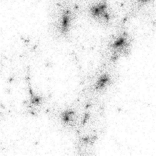
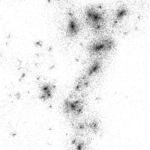
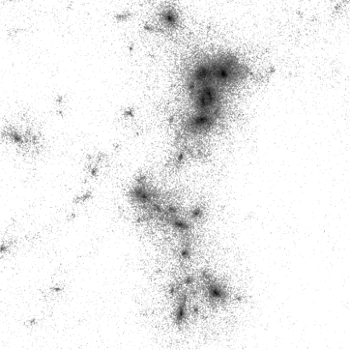
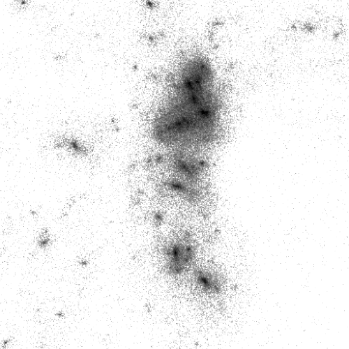
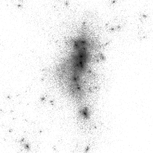
Figure 1.— The projected density in a cube $10\,h^{-1}$Mpc on a side centered on the final position of the second most massive halo in the $512^{3}$ particle simulation. The 9 panels are equally spaced in conformal time from $z=1.5$ to $z=0$. The grey scale is logarithmic, running from $10^{2}$ to $10^{5}$ times the mean density.

3. Simulations

Numerical simulations give qualitative support to the predictions of the Press-Schechter theory, with small modifications noted at both the high and low mass ends. The current state of the art in numerical simulations aimed at elucidating these departures is the work of JFWCCECY. Independent confirmations of the JFWCCECY result have been published recently by White HaloMass (2001), Zheng et al. ZTWB (2002) and Hu & Kravtsov HuKra (2002). In this section we discuss the numerical simulations we have done to investigate the dependence of the result on the mass definition chosen. The reader not interested in the numerical details is urged to skip to §4.

3.1. N-body runs

We have performed a suite of N-body simulations in order to better constrain the mass/multiplicity function (see Appendix for details of the code). The first set we used to tune our fitting function, the rest were used as independent checks. Throughout we have tried to focus primarily on the high-mass end of the mass function, which is of the most use for studies of clusters of galaxies.

Since the primary consideration is one of volume, we have run numerous small simulations rather than one very large one. The small simulations were chosen to have sufficient dynamic range and mass resolution to well resolve a low mass cluster halo. Specifically we ran a number of $150^{3}$ particle simulations of three different CDM models, each in a $200h^{-1}$Mpc box (see Table 1 for more details). Each simulation represents a reasonable cosmological volume, so as not to bias the high mass end of the mass function, while maintaining enough mass and force resolution to identify the relevant halos.

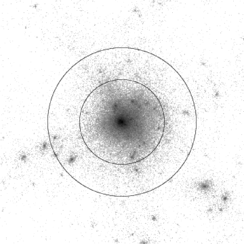
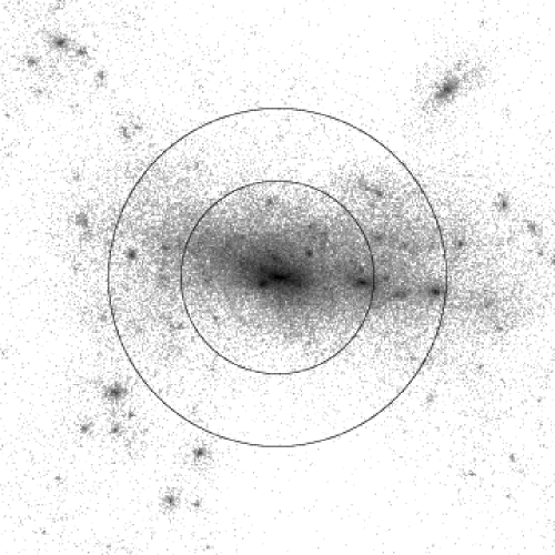
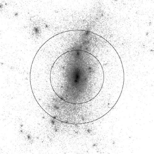
Figure 2.— The projected density in a cube $10\,h^{-1}$Mpc on a side centered on the second most massive halo in the $512^{3}$ particle simulation. The 3 panels are projections down the $x$, $y$ and $z$ axes of the box. The grey scale is logarithmic, running from $10^{2}$ to $10^{5}$ times the mean density. The solid circles show $r_{200c}\simeq 1.74\,h^{-1}$Mpc (inner) and $r_{180b}=r_{54c}\simeq 3.04h^{-1}$Mpc (outer). Within $r_{180b}$ the material exhibits a wide range of density contrasts. Note that the halo is neither isolated nor spherical, and has quite a bit of substructure.

Because it provides a reasonable fit to a wide range of observations, we first simulated a ‘concordance’ $\Lambda$CDM model which has $\Omega_{\rm m}=0.3$, $\Omega_{\Lambda}=0.7$, $H_{0}=100\,h\,{\rm km}{\rm s}^{-1}{\rm Mpc}^{-1}$ with $h=0.67$, $\Omega_{\rm B}=0.04$, $n=1$ and $\sigma_{8}=0.9$ (corresponding to $\delta_{H}=5.02\times 10^{-5}$). We call this model 1. We then changed the model in each of two ‘orthogonal directions’. First we changed the mapping between length scale and mass, by changing $\Omega_{\rm m}$ from 0.3 to 1, while holding the present day power spectrum fixed (model 2). Then we changed the normalization of the power spectrum, $\sigma_{8}$, while holding the cosmology and shape of the power spectrum fixed (model 3). Finally we ran a model with a different spectral shape and normalization as a cross check. Model 4 had $\Omega_{\rm m}=0.35=1-\Omega_{\Lambda}$, $\Omega_{\rm B}h^{2}=0.02$ and $h=0.65$ with $\sigma_{8}=0.8$. Of the models the first has the fewest clusters per unit volume, so we ran more realizations of this model than the other three.

Model	$\Omega_{\rm m}$	$\sigma_{8}$	$N_{\rm box}$	$V_{\rm tot}$	$m_{\rm part}$	$1+z_{\rm ic}$
1	0.30	0.9	15	120	1.97	40
2	1.00	0.9	10	80	6.58	30
3	0.30	1.0	10	80	1.97	40
4	0.35	0.8	10	80	2.30	40

Table 1The parameters of the simulations run. In each case $N_{\rm box}$ different realizations of the Gaussian initial conditions were run. Each run used a periodic box of side $200\,h^{-1}$Mpc and $150^{3}$ particles. The force softening was of a spline form with a “Plummer equivalent” smoothing length of $50\,h^{-1}$kpc – easily small enough to resolve the halos of interest. In the above volumes are quoted in units of $(100\,h^{-1}{\rm Mpc})^{3}$ and particles masses in units of $10^{11}\,h^{-1}M_{\odot}$.

We also used an ‘independent’ simulation to check our fitting function. The cosmology in this case was slightly different than above, having $\Omega_{\rm m}=0.3$, $h=0.7$ and $\sigma_{8}=1$. The simulation employed $512^{3}$ particles in a $300\,h^{-1}$Mpc with a smoothing length of $20\,h^{-1}$kpc. We can use this simulation to see whether the mass function extrapolates correctly to lower masses (where it becomes a power-law), see §6.

3.2. The group catalogs

From the $z=0$ output of each simulation we produce a halo catalogue by running a “friends-of-friends” group finder (e.g. Davis et al. DEFW (1985)) with a linking length of either $b=0.2$ (in units of the mean interparticle spacing) or $b=0.1$. We can use these two different group catalogs to test the sensitivity of our results to the selection of halos. The FoF algorithm partitions the particles into equivalence classes, by linking together all particle pairs separated by less than a distance $b$. We keep all groups above 32 particles, which imposes a minimum halo mass of order $10^{13}h^{-1}M_{\odot}$. [FoF groups with more than 32 particles are known to be robust.] The FoF algorithm as we have defined it cannot be used to address sub-structure in the halos that we find, but for our purposes this will not be a serious limitation as the P-S formalism also completely neglects sub-structure.

Several other group finders exist which we could have used in addition to the FoF algorithm. Some of these begin with groups defined in a FoF manner while some find a partition of the particles in a completely different way. Luckily, an exploration of all of these different group finders will turn out to be unneccesary. For most of the mass estimates defined in §4 the precise group finding algorithm is unimportant. We shall show later that the mass functions obtained with two different FoF groups, with radically different partitionings of the particle distribution, are almost identical. This may be telling us that the physical properties of the group which we are calculating, the ‘total mass’, are independent of the details of how the group is originally found as an overdensity in three dimensional space.

In order to define the mass it will be very useful to have a halo center. We define the center of a halo as the position of the potential minimum, calculating the potential using only the particles in the FoF group. This proved to be more robust than using the center of mass, as the potential minimum coincided closely with the density maximum for all but the most disturbed clusters. Additionally, the position of the center was very insensitive to the presence or absence of the particles near the outskirts of the halo, and thus to the precise linking length used.

4. The mass of a halo

As remarked earlier, since the objects formed in a hierarchical model have no clear boundary, all mass definitions are a matter of convention. For each halo in each catalog we computed 8 different definitions of mass. As we shall see later, it is only those definitions which encompassed the majority of the virialized material (§5) which will turn out to be useful for our purposes, and the best shall be $r_{180b}$.

First we used the ‘FoF mass’, simply the number of particles in the group times the particle mass. With $b=0.2$, this definition is the one used by JFWCCECY, for which they found a universal mass function. By considering the mean number of particles in a sphere of radius $b$ one can argue that (if all particles have the same mass) FoF groups are bounded by a surface of density $3/(2\pi b^{3})\simeq 60$ times the background. If all groups were spherical and singular isothermal spheres, this would imply a mean density inside the FoF group of roughly $180$ times the background density or $180\Omega_{\rm m}$ times the critical density. In practice there is a very large scatter about this value. We also use the sum of the particles in the $b=0.1$ groups.

Motivated by the self-similarity exhibited by halos in simulations we also define the mass from a spherically averaged profile about the cluster center. Specifically we define $M_{\Delta}$ as the mass contained within a radius $r_{\Delta}$ inside of which the mean interior density is $\Delta$ times the critical density

$$\int_{0}^{r_{\Delta}}r^{2}dr\ \rho(r)={\Delta\over 3}\rho_{\rm crit}r_{\Delta}^{3}\qquad.$$ (6)

The ‘virial mass’ from the spherical top-hat collapse model would then be simply $M_{\Delta_{\rm c}}$. We shall refer to this mass as $M_{{\rm th-vir}}$ rather than the somewhat vague term virial mass. Since $\Delta_{\rm c}\simeq 200$ in a critical matter density cosmology, many authors mean by ‘virial mass’, $M_{200}$. This is in fact the most common definition. We shall write this $M_{200c}$ to make explicit the fact that it is with respect to the critical density. We shall also consider $M_{500c}$, which has the advantage that it probes material at sufficiently small radii that it is often directly accessible to X-ray observations.

In the above we have followed common usage and measured the mean interior density contrast to the critical density. This has historically been motivated by (a) considerations based on the virial theorem, which provides estimates of the halo velocity dispersion and ‘temperature’, in which the critical density provides a natural scale and (b) because it requires no assumptions about the cosmological parameters (beyond $h$) in its definition. More recent work, specifically JFWCCECY, has suggested that the halo mass function may be universal if masses are measured within a fixed density contrast measured not with respect to the critical density, but with respect to the background density. We shall follow their lead and also calculate $r_{180b}$, where the mean interior density is $180$ times the background density. Note that while the mass function may be more universal with this definition, it comes with an associated price from an observational point of view: it introduces a dependence on an assumed $\Omega_{\rm m}$ in the definition.

Unfortunately both the FoF mass with $b=0.2$ and $r_{180b}$ encompass a very wide range of material (see Fig 2), far beyond what can usually be observed and into the region where the profiles start to show significant scatter from halo to halo. For a cluster mass halo, $r_{180b}$ can be 75% larger than the most widely used $r_{200c}$. For this reason we shall also consider $M_{500b}$ and $M_{1000b}$, which require less of an extrapolation.

In cases where we use a small linking length and a large $r_{\Delta}$ it is possible that two halos overlap. Since our definition of mass for each halo includes all of the mass within $r_{\Delta}$, not just that associated with the FoF halo itself, this can result in us double-counting the mass in the overlap region. This is an unfortunate side-effect of a mass estimator based on spherical averages for objects which are neither spherical nor isolated. To avoid this we cull from each run the smaller of two halos whose centers are closer than the sum of the ‘virial’ radii. This procedure is then relatively insensitive to the linking length used to define the original halos. If we had used a larger linking length and ‘merged’ the extra halo with the larger one (removing it from out list), the mass assigned to the combined halo would still be that within $r_{\Delta}$ of the potential minimum of the combined group – presumably the potential minimum of the larger mass group – and thus be the mass originally assigned to the larger of the two groups. If we do not perform this culling step then we find a significant excess of low mass objects compared to the analytic predictions. With the culling the mass function becomes almost totally insensitive to the original group finder parameters.

The need for this step is more than just a technical issue. It stems from the fact that in hierarchical models halos are rarely isolated, but are often found in various stages of merging or accretion. Observers often remove from their samples systems which they deem to be interacting too strongly or too recently. This can introduce a ‘bias’ in the mass function. Rather than attempt to quantify how ‘disturbed’ various halos are or whether there is observational evidence for interaction which would cause them to be removed from any particular sample, we have chosen to apply a criterion that can be equally well applied in simulations and observations: we omit the smaller of any two systems whose virial radii overlap. The fraction of the halos culled in each of the models is relatively small. For example in Model 1 for the $b=0.2$ halos the culled fraction is less than 1% for all of the mass definitions. For $b=0.1$ it is 15% for $M_{180b}$, $8\%$ for $M_{\rm th-vir}$ and around 1% or less for the other mass definitions. How closely our treatment mimics the selection of individual objects in current samples is unclear. As we demand increasing accuracy in our comparison between theory and observation this issue will need to be revisited.

5. The virial region

Our definition of a halo is primarily one of density contrast. An alternative definition is that a halo contains material which has broken away from the universal expansion and is (at least approximately) in virial equilibrium. As we shall see below, it is only for density thresholds where these two definitions roughly coincide that one obtains a nearly universal mass function. Since the virial region encompasses such a large volume of space, this will require us to investigate extrapolations from the inner, easier to measure, regions.

As a first step it is interesting to ask how well the spherical top-hat collapse model approximates the messy formation process of a cluster in a hierarchical model (see Fig. 1). To investigate this we have looked at the five most massive clusters in the $512^{3}$ particle simulation described earlier. For each cluster we calculate the mean radial velocity, $\bar{v}_{r}(r)$, and the velocity dispersion, $\sigma(r)$, in bins containing 5000 particles from the center out to 3 times the virial radius predicted by the top-hat model ($r_{101}$ for $\Omega_{\rm m}=0.3$). The results are shown in Fig. 3.

Figure 3.— The radial velocity (dotted) and velocity dispersion (dashed) profiles of the 5 most massive clusters in the $512^{3}$ simulation described in the text. Each cluster has ${\cal O}(10^{5})$ particles and $M_{200c}>10^{15}\,h^{-1}\,M_{\odot}$. Points are plotted every 5000 particles in radius out to $3\times$ the top-hat virial radius. The velocities are all normalized to the 3D velocity dispersion of the dark matter within $r_{\rm th-vir}$.

Fig. 3 shows that the clusters are roughly isothermal, with a velocity dispersion profile that peaks near the break radius (where the density profile has a slope of $-2$). Inside of the virial radius the mean velocity is close to zero, in units of the 3D velocity dispersion $\sigma_{\rm vir}$. Just outside the virial radius the transition from ‘virialized’ material to in-flowing material ($\bar{v}_{r}<0$) is clearly seen in all 5 clusters. Thus it seems that the ‘virial radius’ is predicted within a factor of 2 by the top-hat model, though the clusters exhibit some scatter. The radius $r_{180b}$ is only 30% larger than $r_{\rm th-vir}$ for a cluster mass halo in this cosmology, so within the scatter we could take the ‘virial’ radius to be $r_{180b}$ also. Using a higher density contrast than $\Delta_{c}$, e.g. $M_{200c}$ or $M_{500c}$, would clearly underestimate the transition radius for all of the clusters.

To get a feel for the translation between density contrast and ‘size’ for a rich cluster, we can make use of the universal density profile of Navarro, Frenk & White NFW (1996). These authors defined the virial radius as $r_{200c}$ and density contrasts with respect to critical. The universal form of the density profile is

$${\rho(r)\over\rho_{\rm crit}}\propto{1\over x(1+x)^{2}}$$ (7)

where $x=r/r_{s}$ is a scaled radius and $r_{s}$ describes the transition from $r^{-1}$ to $r^{-3}$ in the profile. We show the radius within which the mean density is $\Delta$ times the critical density in Fig. 4 for a rich cluster with $M_{200c}=10^{15}\,h^{-1}M_{\odot}$ and a concentration $c\equiv r_{200c}/r_{s}=5$. Note that for $\Omega_{\rm m}=0.3$, $r_{180b}=r_{54c}\simeq 2.8\,h^{-1}$Mpc. For lower $\Omega_{\rm m}$ it would exceed $3\,h^{-1}$Mpc.

Figure 4.— The radius $r_{\Delta}$ within which the mean density is $\Delta$ times the critical density for an NFW halo with $M_{200c}=10^{15}\,h^{-1}M_{\odot}$ and $c=5$. For $\Omega_{\rm m}=0.3$ the ‘universal’ density contrast of $r_{180b}$ is at $r_{54c}\simeq 2.8\,h^{-1}$Mpc.

6. A universal mass function?

Figure 5.— The multiplicity function vs. the peak height $\nu^{2}$ for our 3 models and for 6 of our 8 mass definitions. Open circles are Model 1, open squares Model 2 and triangles Model 3. The solid line is the S-T fitting function. The panels are labeled with the halo mass definition used. This indicates to what extent the mass functions are indeed universal.

Given a (possibly culled) set of halos each with a known mass, we wish to find a fitting function to the mass/multiplicity function. As a first step we check whether the mass functions do indeed form a ‘universal’ multiplicity function by plotting

$$N(>\nu)\equiv\int_{\nu}^{\infty}{M\over\bar{\rho}}{dn\over d\nu}d\nu$$ (8)

vs. the peak height $\nu^{2}$ (Fig. 5). As we can see, for the 3 models shown, it is a good approximation to assume that all of these mass functions come from a universal multiplicity function for the FoF halos with $b=0.2$. The universal form is quite well fit by the Sheth & Tormen form of Eq. (5). This confirms the earlier work of JFWCCECY.

The mass function is also close to universal if the top-hat virial mass is used, though the agreement is not as good as in the $b=0.2$ case and would need to be checked for a wider range of cosmologies. As noted by JFWCCECY the mass $M_{180b}$ also gives a close to universal mass function. Each of these mass estimators includes the majority of the mass within the virialized region (see Fig. 3).

As expected, the mass function within $r_{200c}$ shows a systematic difference between the $\Omega_{\rm m}=1$ model and the other two. This is because the mass is defined interior to a density contrast which doesn’t scale with the background density.

Of particular interest is the case of $M_{1000b}$. Here the mass is defined in terms of a density contrast with respect to the background density (like the ‘universal’ $M_{180b}$), but at a higher density. This region of the halo is more amenable to observation. However we note that as we increase the density threshold, focusing on the inner regions of the halos, the universality of the mass function degrades. [The case $M_{500b}$ is intermediate, and is omitted from the figure.]

Figure 6.— The (interior) mass profiles in scaled units for the halos above $M_{180b}=5\times 10^{14}\,h^{-1}\,M_{\odot}$ in the 3 models. As before, open circles are Model 1, squares Model 2 and triangles Model 3. The mean and standard deviation of the profiles is shown. Note that by definition $M(<r_{180b})=180\bar{M}(<r_{180b})$ so there is no scatter in this point.

Figure 7.— The ratio of different mass estimators for clusters with $M_{180b}>5\times 10^{14}\,h^{-1}\,M_{\odot}$ in the 3 models. Solid line is Model 1, dotted Model 2 and dashed Model 3.

We can understand this result by considering the different formation histories of the halos. Fig. 6 shows the average mass profiles of the most massive halos from the 3 models in scaled units. The halos in Model 2, with $\Omega_{\rm m}=1$, form later and thus are less concentrated than the halos in Models 1 and 3. This increases the ratio $M_{1000b}/M_{180b}$ (see Fig. 7) or $M_{1000b}/M_{200c}$. On an object by object basis this scatter is fairly large. This is unfortunate since it is precisely the inner regions which are most amenable to observation! Thus the mass estimators for which the mass function is close to universal are those which require an extrapolation beyond the observed region (out to $2-3\,h^{-1}$Mpc), and this extrapolation is quite sensitive to both the cosmology and the particular formation history of the halo under consideration.

Figure 8.— The multiplicity function vs. the peak height $\nu^{2}$, divided by the fitting function of Eq. (5), for $M_{180b}$. Open circles and stars are Model 1 with $b=0.2$ and $b=0.1$ respectively. Open squares and 3-pointed crosses Model 2, triangles Model 3 and plusses and diamonds Model 4 (with worse statistics at the high mass end). The 4-pointed crosses are the results from the $512^{3}$ run of a slightly different model (see text). At the high mass end ($\nu\to\infty$) our statistics become very poor.

Figure 9.— The multiplicity function vs. the peak height $\nu^{2}$, divided by the fitting function of Eq. (5) as above. Here we have converted from $M_{500c}$ to $M_{180b}$ assuming the halos are all of the NFW form with $c=5$. Open circles and stars are Model 1 with $b=0.2$ and $b=0.1$ respectively. Open squares and crosses Model 2, triangles Model 3 and plusses and diamonds Model 4.

We show in Fig. 8 the mass functions on a linear scale. We report the results as a ratio of the N-body results to the integral of Eq. (5) for the case of $M_{180b}$. Each of the four models is represented by two sets of points, one where the halos are initially found with a linking length of $b=0.2$, and the other with $b=0.1$. As we can see there is almost no dependence on the initial group finder used in this case. As a cross check we also show on this linear scale the mass function from the $512^{3}$ particle simulation in the $300\,h^{-1}$Mpc box. This run has much higher mass and force resolution than the majority of the runs used here, and a slightly different cosmology i.e. spectral shape and normalization on the scales of interest. The total volume is however smaller, so the statistics at the $\nu\to\infty$ end are much poorer. However it makes a good ‘independent’ check of the universality of the mass function. The scatter between the models is at the $\pm 20\%$ level.

We also show, on the same linear scale, the results of converting between different spherically averaged mass profiles in Fig. 9. Following White HaloMass (2001) we show in particular what happens if one constructs the mass function by measuring $M_{500c}$, converting this to $M_{180b}$ using an NFW profile with $c=5$. We make no correction for the large scatter we saw in the detailed comparisons above, we simply apply a numerical rescaling. For $\Omega_{\rm m}=0.3$ the conversion is $M_{180b}\simeq 2.0M_{500c}$ while for $\Omega_{\rm m}=1$ the conversion is $M_{180b}\simeq 1.4M_{500c}$. As we can see, while the conversion shows a lot of scatter it introduces no major bias and the mass functions so constructed are close to universal. Such a procedure was followed, in reverse, by Pierpaoli et al. PSW (2001) and Seljak Sel (2002) for example. A more complicated conversion along the same lines has been provided by Hu & Kravtsov HuKra (2002). This is very encouraging because it means that, while $M_{180b}$ cannot reliably be measured on an object-by-object basis, a noisy estimator of it can be easily constructed which turns out to be good enough to construct the ‘universal’ mass function. The outlier is Model 4 which was already known to be discrepant in Fig. 8. The rescaling has made it more discrepant from the mean, indicating that this procedure is not without its flaws, but even so the mass function is predicted to 30% over much of the range.

7. Fitting the mass function

For completeness we would like to find a fit to the simulated mass functions (Figs. 10, 11). Since to a very good approximation the mass function is independent of the clustering of the halos, we can do this using the Poisson model. First we bin the halos in mass using a large enough number of bins that no bin contains more than 1 halo. We use bins equally spaced in $\log M$. Then we maximize the (log) likelihood

$$-\log{\cal L}=\sum_{i\in{\rm full}}\log\mu_{i}-\sum_{j\in{\rm all}}\mu_{j}+{\rm const}$$ (9)

where the sum on $i$ is over bins containing $1$ particle, the sum on $j$ is over all the bins and

$$\mu\equiv{dn\over d\log M}\,\Delta\log M\ll 1$$ (10)

is the mean number of halos per bin assuming a mass function $dn/d\log M$. This method has the advantage of being independent of the chosen bin width and correctly taking into account the Poisson statistics of the rare halos at the high mass end.

We have chosen to use the modification to the Press-Schechter formula, Eq. (5), proposed by Sheth & Tormen SheTor (1999), but to allow $a$ and $p$ to be free parameters. We maximize the likelihood for $a$ and $p$ fitting over the range $M_{0}=10^{14}\,h^{-1}M_{\odot}$ to $M_{1}=3\times 10^{15}\,h^{-1}M_{\odot}$. The results of this procedure are shown in Table 2. We found that the fit was somewhat sensitive to the particular value of $M_{0}$ chosen, indicating that the numerical mass function wasn’t perfectly fit by the form of Eq. (5). Using the higher resolution simulation we found that the fitting function tended to overpredict the abundance of halos with $\nu^{2}<1/2$, by a factor of almost 2 for the lowest mass halos we could probe. Since we concentrate here on the more massive end of the mass function we did not attempt to correct for this.

There is a fair degree of variation in the best fit parameter $a$, while $p$ is close to constant. This is because $p$ essentially controls the slope of the low-mass ($\nu\sim 1$) end of the mass function which is very nearly the same for all the estimators. We obtain reasonable agreement with Sheth & Tormen SheTor (1999) for the conventional mass estimator $M_{200c}$ for the critical density cosmology for example, but $a$ is significantly smaller using the $b=0.2$ FoF mass and significantly larger using the $b=0.1$ FoF mass. Generally $a$ increases as the mass estimator probes material primarily at a higher density contrast.

For the ‘universal’ contrast of $M_{180b}$ calculated directly from the halo mass distribution we found better agreement with the numerical results in all cases if we lowered $a$ slightly below the $0.7$ found by Sheth & Tormen for this mass estimator. This is the opposite of the claim of Hu & Kravtsov HuKra (2002) that $a$ should be increased to $0.75$ when using $M_{180b}$. On the other hand for the one example we studied in detail where we converted from a mass measured within $r_{500c}$ to one within $r_{180b}$ using an NFW profile with $c=5$, the best fitting $a$ was slightly higher than $0.7$. The difference in the mass functions so produced, as $a$ is changed from $0.65$ to $0.75$, is at approximately the same level of the scatter from model to model shown in Fig. 8. Thus these fluctuations could be reflecting an intrinsic limit to how well we can determine our fitting function.

Figure 10.— Mass functions for the 3 models, 2 linking lengths and 4 of the mass definitions. Left panels are for $b=0.2$, right for $b=0.1$. Top to bottom are Models 1, 2 and 3. The open squares are FoF mass, solid triangles $M_{\rm th-vir}$, open circles $M_{200c}$ and crosses $M_{500c}$. In the first panel the solid line is the Press-Schechter prediction, and the dashed line the fit to the Virgo simulations. The solid line is suppressed in the other panels.

Figure 11.— Mass functions for the 3 models, 2 linking lengths and 4 of the mass definitions. Left panels are for $b=0.2$, right for $b=0.1$. Top to bottom are Models 1, 2 and 3. The open squares are FoF mass, solid triangles $M_{180b}$, open circles $M_{500b}$ and crosses $M_{1000b}$. In the first panel the solid line is the Press-Schechter prediction, and the dashed line the fit to the Virgo simulations. The solid line is suppressed in the other panels.

		$b=0.2$		$b=0.1$
Sim	$\Delta$	$a$	$p$	$a$	$p$
1	FoF	0.64	0.34	1.17	0.31
1	$\Delta_{\rm c}$	0.79	0.32	0.79	0.32
1	200c	0.98	0.30	0.98	0.31
1	500c	1.36	0.29	1.35	0.30
1	180b	0.67	0.33	0.66	0.33
1	500b	0.89	0.31	0.89	0.31
1	1000b	1.13	0.29	1.12	0.30
2	FoF	0.64	0.32	1.41	0.27
2	$\Delta_{\rm c}$	0.66	0.29	0.65	0.29
2	200c	0.70	0.29	0.69	0.29
2	500c	1.07	0.26	1.05	0.27
2	180b	0.67	0.29	0.65	0.29
2	500b	1.07	0.26	1.05	0.27
2	1000b	1.48	0.25	1.45	0.26
3	FoF	0.64	0.34	1.20	0.30
3	$\Delta_{\rm c}$	0.76	0.31	0.76	0.31
3	200c	0.97	0.30	0.96	0.31
3	500c	1.38	0.28	1.37	0.29
3	180b	0.64	0.33	0.64	0.33
3	500b	0.87	0.30	0.86	0.31
3	1000b	1.13	0.29	1.12	0.30

Table 2Mass function parameters for the different cosmologies and different mass definitions (see text).

8. Clustering and the mass function

Throughout we have assumed that the number of clusters in a given volume is simply Poisson distributed about a mean value given by the mass function. In principle however the positions of clusters are correlated and this can induce non-Poisson fluctuations (Evrard et al. EvrHubble (2002); for a simple analytic model see Hu & Kravtsov HuKra (2002)). We expect this effect to be small when the objects are rare and the sample region is large compared to the cluster correlation length $r_{0}\sim{\cal O}(10\,h^{-1}{\rm Mpc})$ (see e.g. Peebles LSSU (1980)) but we can quantify its effect using numerical simulations.

Hu & Kravtsov HuKra (2002) have investigated the additional scatter in the normalization that arises from including clustering using a simple analytic model where clusters are biased tracers of the linear density field. We shall investigate this effect using the $z=0$ group catalog from the Hubble Volume Simulation of a $\Lambda$CDM model run by the Virgo Supercomputing Consortium (JFWCCECY). To quantify the scatter in the mass function, we shall compute the best fitting power spectrum normalization, $\sigma_{8}$, to 1000 random sub-volumes of the simulation, using the maximum likelihood method described above. We hold the other parameters fixed at their fiducial values for simplicity. Each sub-volume is centered on a random point in the simulation, which can be chosen as the center using the periodicity of the box. Then all clusters are kept which have $M$ above a threshold mass, are closer than $R$ to the center of the box and would have $|b|>30^{\circ}$ if the box $x-y$ plane was oriented parallel to the galactic plane. This roughly mimics a volume limited X-ray survey out to depth $R$ sensitive to the most massive, and therefore most clustered but rarest galaxy clusters. We choose two mass thresholds, $10^{14}\,h^{-1}\,M_{\odot}$ and $3\times 10^{14}\,h^{-1}\,M_{\odot}$. The scatter expected from a Poisson distribution can be estimated using the same procedure, except that we first randomize the positions of the halos.

Fig. 12 shows the standard deviation in $\sigma_{8}$, in units of the mean value, as a function of sampled volume for the ‘clustered’ and ‘Poisson’ cases. We checked that estimating the variance directly or from the difference between the $16^{\rm th}$ and $84^{\rm th}$ percentiles of the distribution gave similar results. For all volumes studied the variance in $\sigma_{8}$ is increased by clustering over the simple Poisson expectation (Evrard et al. EvrHubble (2002)), however for volumes of interest ($R_{\rm max}>300\,h^{-1}$Mpc) both the Poisson variance and the increase due to clustering are almost negligible compared to the other errors (see e.g. Table 6 of Pierpaoli et al. PSW (2001)). We checked explicitly that there was no bias in the mean introduced by the neglect of clustering in the analysis.

Figure 12.— The standard deviation of $\sigma_{8}$, in units of the mean, as a function of survey radius. We plot a quantity, half the difference between the $16^{\rm th}$ and $84^{\rm th}$ percentiles of the distribution, which is slightly less sensitive to outliers than the variance; but the results would be almost identical if we had plotted the variance. Solid lines indicate the width of the distribution including the clustering of clusters, dashed lines are for the randomized sample. Lines joining open squares are for $M>3\times 10^{14}\,h^{-1}\,M_{\odot}$ and joining solid triangles for $M>10^{14}\,h^{-1}\,M_{\odot}$.

9. Conclusions

The multiplicity function, a measure of the number of halos per comoving volume element per unit mass, is one of the central predictions of a model of structure formation. Dark matter dominated models in which structure evolves hierarchically from gaussian initial conditions predict a mass function which is nearly universal if expressed in the right units. This is only true for a narrow class of mass estimators, and is specifically not true for the estimators which have been most commonly used up until now.

Given the complicated process by which halos form in hierarchical models, the role of mergers and prevalence of sub-structure, it is highly convenient that the mass function (in scaled units) is so close to universal. We have provided fitting functions to the mass function from N-body simulations for 8 different mass estimators, and shown how one can convert between them. We have found that measuring the mass of a halo using one definition and using a simple average spherical profile, such as the NFW profile, to convert to the ‘universal’ $M_{180b}$ provides a remarkably good method of estimating the mass function, even though individual halos show a large scatter among different mass estimates.

Finally let us remark upon the small non-universality in the multiplicity function, which can lead to misestimates of the true mass function if one uses a fitting function like Eq. (5). Neglecting the factor $d\log\sigma/d\log M$ in the mass function, making an error of $\delta n/n$ in the number density per $\log M$ at mass $M$ translates into an error of $(\nu^{2}-1)^{-1}\delta n/n$ in the normalization $\delta\sigma/\sigma$. So for a typical cluster, with $\nu\sim 2-3$, the scatter in the mass function doesn’t limit our knowledge of $\sigma_{8}$ until the other uncertainties are pushed below ${\cal O}(5\%)$. Thus the non-universality of the mass function is not currently a limitation to using the abundance of rich clusters to determine the normalization of the matter power spectrum. The uncertainties become increasingly important when it comes to using the evolution of the mass function as a probe of $\Omega_{\rm m}$ or the equation of state, $w$, of the dark energy. For the latter, errors on $\sigma_{8}$ approaching the percent level are required. For these ambitious measurements it may not be sufficient to use a simple parameterized form for the multiplicity function. One could either resort to full blown numerical simulations for a grid of models ‘near’ the parameter region of interest or attempt to find a ‘second variable’ which correlates well with the scatter between the simulation results and the P-S predictions. As we approach the level of precision where these effects matter a variety of other effects also become important, including the effects of clustering (see e.g. §8, Evrard et al. EvrHubble (2002), Hu & Kravtsov HuKra (2002)) and how to treat merging systems. It will be a challenge for theorists to keep the ‘theory uncertainty’ below the ‘experimental uncertainty’ with the increasingly rapid advances in observations.

Appendix A The TreePM-SPH code

The simulations in this paper were done using the TreePM-SPH code (White et al. TreePM (2002)) running in fully collisionless mode. We present a brief discussion of the features of the code here for completeness.

The TreePM code was specifically designed to run on distributed memory computers or clusters of networked workstations and evolves dark matter (and gas) in a periodic simulation volume. The code uses the TreePM method of Bagla Bagla (1999) for the gravitational force and smoothed particle hydrodynamics (SPH; Lucy Luc (1977) and Gingold & Monaghan GinMon (1977)) in its ‘entropy’ formulation (Springel & Hernquist SprHer (2002)) to compute the hydrodynamic forces. The (collisionless) dark matter component and (collisional) gas are assumed to interact only through gravity. The code is written in standard C and uses the Message Passing Interface (MPI) communications package, making it easily portable to a variety of parallel computing platforms. It performs dynamical load balancing and scales efficiently with increasing numbers of processors. It will run on an arbitrary number of processors, though it is slightly more efficient if the number is a power of two.

The particles are integrated using a second order leap-frog method, where the relevant positions, energies etc are predicted at a half time step and used to calculate the accelerations which modify the velocities. The time step is dynamically chosen as a small fraction (depending on the smoothing length) of the local free-fall time. Particles have individual time steps so that the code can handle a wide range in densities efficiently. To increase speed the force on any given particle is computed in two stages. The long-range component of the force is computed using the PM method, while the short range component is computed from a global tree. In this manner the code is similar in spirit to P³M except that the short range force, being computed from a tree, scales as $N\log N$ rather than $N^{2}$.

Rather than a Plummer potential we use a spline softened force. We use the same smoothing kernel for the gravity and SPH calculations. The long-range force is smoothed on 2 grid cells, and the opening criterion for the tree is set to achieve $1\%$ accuracy in the short-range force. With these standard parameters the 90th percentile force error is 1.2% for lightly clustered distributions while for very uniform distributions the 90th percentile error rises slightly to 1.9%, as the total force is smaller and the short range force contributes less.

We have made extensive comparisons of the code described here to other codes described in the literature, building on the many test problems that those codes have been shown to satisfy. In particular we have compared TreePM extensively with Gadget (Springel, Yoshida & White SprYosWhi (2001)). Details of these comparisons, along with results from self-similar evolution, hydrodynamics tests including the sod shock tube, the Santa-Barabara cluster comparison project (Frenk et al. Fre (1999)) etc can be found in White, Springel & Hernquist TreePM (2002).

References

- (1) Bagla J., 1999, preprint [astro-ph/9911025]
- (2) Bond J.R., Cole S., Efstathiou G., Kaiser N., 1991, ApJ, 379, 440
- (3) Bond J.R., Myers S., 1996, ApJS, 103, 41
- (4) Bower R.J., 1991, MNRAS, 248, 332
- (5) Cole S., Kaiser N., 1989, MNRAS, 237, 1127
- (6) Davis M., Efstathiou G., Frenk C.S., White S.D.M., 1985, ApJ, 292, 371
- (7) Efstathiou G., Frenk C.S., White S.D.M., Davis M., 1988, MNRAS, 235, 715
- (8) Efstathiou G., Rees M., 1988, MNRAS, 230, 5P
- (9) Evrard A.E., et al., 2002, ApJ, in press [astro-ph/0110246]
- (10) Frenk C.S., et al., 1999, ApJ, 525, 554
- (11) Gelb J., Bertschinger E., 1994, ApJ, 436, 467
- (12) Gingold R.A., Monaghan J.J., 1977, MNRAS, 181, 375
- (13) Hu W., Kravtsov A., 2002, preprint [astro-ph/0203169]
- (14) Jenkins A., Frenk C.S., Pearce F.R., Thomas P.A., Colberg J.M., White S.D.M., Couchman H.M.P., Peacock J.A., Efstathiou G., Nelson A.H., 1998, ApJ, 499, 20
- (15) Jenkins A., Frenk C.S., White S.D.M., Colberg J.M., Cole S., Evrard A.E., Couchman H.M.P., Yoshida N., 2001, MNRAS, 321, 372 (JFWCCECY)
- (16) Lacey C., Cole S., 1993, MNRAS, 262, 627
- (17) Lacey C., Cole S., 1994, MNRAS, 271, 676
- (18) Lucy L., 1977, AJ, 82, 1013
- (19) Mo H.J., White S.D.M., 1996, MNRAS, 282, 347
- (20) Navarro J., Frenk C.S., White S.D.M., 1996, ApJ, 462, 563
- (21) Peacock J.A., 1999, Cosmological Physics, Cambridge University Press, Cambridge
- (22) Peacock J.A., Dodds S.J., 1996, MNRAS, 280, L19
- (23) Peacock J.A., Heavens A., 1990, MNRAS, 243, 133
- (24) Peebles, P.J.E., 1980, The Large-Scale Structure of the Universe, Princeton University Press, Princeton, §36.
- (25) Peebles, P.J.E., 1993, Principles of Physical Cosmology, Princeton University Press, Princeton, chapter 25.
- (26) Pierpaoli E., Scott D., White M., 2001, MNRAS, 325, 77
- (27) Press W.H., Schechter P., 1974, ApJ, 187, 452
- (28) Seljak U., 2002, preprint [astro-ph/0111362]
- (29) Sheth R., Tormen G., 1999, MNRAS, 308, 119
- (30) Springel V., Hernquist L., 2002, MNRAS, in press [astro-ph/0111016]
- (31) Springel V., Yoshida N., White S.D.M., 2001, New Astronomy 6, 79 [astro-ph/0003162]
- (32) White M., 2001, A&A, 367, 27 [astro-ph/0011495]
- (33) White M., Springel V., Hernquist L., 2002, in preparation.
- (34) White S.D.M., Efstathiou G., Frenk C., 1993, MNRAS, 262, 1023
- (35) Zheng Z., Tinker J.L., Weinberg D.H., Berlind A.A., 2002, preprint [astro-ph/0202358]