Analysis of colour-magnitude diagrams of rich LMC clusters: NGC 1831

We present the analysis of a deep colour-magnitude diagram (CMD) of NGC 1831, a rich star cluster in the LMC. The data were obtained with HST/WFPC2 in the F555W ($\sim$ V) and F814W ($\sim$ I) filters, reaching $m_{555}\sim 25$. We discuss and apply a method of correcting the CMD for sampling incompleteness and field star contamination. Efficient use of the CMD data was made by means of direct comparisons of the observed to model CMDs. The model CMDs are built by an algorithm that generates artificial stars from a single stellar population, characterized by an age, a metallicity, a distance, a reddening value, a present day mass function and a fraction of unresolved binaries. Photometric uncertainties are empirically determined from the data and incorporated into the models as well. Statistical techniques are presented and applied as an objective method to assess the compatibility between the model and data CMDs. By modelling the CMD of the central region in NGC 1831 we infer a metallicity $Z=0.012$, $8.75\leq\log(\tau)\leq 8.80$, $18.54\leq(m-M)_{0}\leq 18.68$ and $0.00\leq E(B-V)\leq 0.03$. For the position dependent PDMF slope ($\alpha=-\mathrm{d}\log\Phi(M)/\mathrm{d}\log M$), we clearly observe the effect of mass segregation in the system: for projected distances $R\leq 30$ arcsec, $\alpha\simeq 1.7$, whereas $2.2\leq\alpha\leq 2.5$ in the outer regions of NGC 1831.

1 Introduction

The Large Magellanic Cloud (LMC) presents three essential characteristics that make it an excellent complementary laboratory for studying the formation and evolution of galaxies and stellar systems in general: a) it is close to the Galaxy; b) it has markedly different morphological, chemical and kinematical properties from our Milky Way; c) it presents a large variety of stellar clusters, displaying distinct physical characteristics among themselves and when compared to those in the Galaxy (Westerlund 1990). Due to the diversity in ages and metallicities, LMC clusters are found at distinct evolutionary stages (Westerlund 1990, Olszewski et al. 1991). The determination of a cluster’s present physical properties, such as density profile, shape, internal velocity distribution and its position dependent Present Day Mass Function (PDMF), provide us with essential links needed to assess the role of gravitational dynamics, including effects of mass segregation and stellar evaporation (Heggie & Aarseth 1992, Spurzem & Aarseth 1996, de Oliveira et al. 2000). Thus, once these present properties are known, modelling techniques like N-body simulations allow us to recover the initial conditions under which clusters formed (Goodwin 1997, Vesperini & Heggie 1997, Kroupa et al. 2001). In this context, the initial mass function (IMF) and its possible universality, are key pieces in the study of stellar contents of distant galaxies (Kroupa 2001).

Through the analysis of colour-magnitude diagrams (CMDs) one has a great variety of physical information about a cluster. Isochrone fits help constraining the system’s age, metallicity, distance and reddening. Furthermore, observational luminosity functions (LFs) have allowed derivation of the stellar mass function (Elson et al. 1995, De Marchi & Paresce 1995, Santiago et al. 1996, Piotto et al. 1997, de Grijs et al. 2002a). However, the transformation of luminosity into mass depends on age and metallicity, the uncertainties in these parameters being therefore incorporated into the inferred mass function. Besides, the theoretical uncertainties in the mass-luminosity relation itself, specially for the low-mass stars (Piotto et al. 1997, Baraffe et al. 1998), added to the effect of unresolved binarism, further hampers real mass function determination through observational luminosity functions.

From both observational and theoretical points of view, the advent of the Hubble Space Telescope (HST), associated with the constant improvement in theories of stellar interiors, atmospheres and evolution, require ever more sophisticated methods of CMD analysis. In this context, computational modelling techniques have allowed a wider use of CMDs as tools to constrain physical properties of stellar populations and systems. Model CMDs, along with statistical methods of comparing them to observed ones, have been useful means to investigate the star formation history within a galaxy (Gallart et al. 1996, Gallart et al. 1999, Hernandez et al. 1999, Holtzman et al. 1999, Hernandez et al. 2000) or to constrain structural parameters and the stellar luminosity function in the Milky Way (Kerber et al. 2001).

With these issues in mind, our work aims at extracting as much physical information as possible about rich LMC clusters, by means of objective comparison of their observed CMDs with artificial ones. The idea is to simultaneously infer PDMF slope, age, metallicity, distance, reddening and unresolved binary fraction for each system studied. The present work introduces the techniques developed for that purpose and shows the results for NGC 1831, one of the richest LMC clusters for which we have deep HST data.

Previous works are evidence of the large difficulties in extracting physical parameters for NGC 1831. Techniques based on CMDs from CCD photometry (Mateo 1987,1988; Chiosi 1989; Vallenari et al. 1992; Corsi et al. 1994), integrated spectroscopy or colours (Bica et al. 1986; Meurer et al. 1990; Cowley & Hartwick 1992; Girardi et al. 1995) and spectroscopy of individual giant stars (Olszewski et al. 1991) were employed with this aim, constraining the values of the main parameters: $8.50\lower 2.15277pt\hbox{$\;\buildrel<\over{\sim}\;$}\log(\tau)\lower 2.15277pt\hbox{$\;\buildrel<\over{\sim}\;$}8.80$ ($300\lower 2.15277pt\hbox{$\;\buildrel<\over{\sim}\;$}\tau\lower 2.15277pt\hbox{$\;\buildrel<\over{\sim}\;$}650$ Myr); $0.002\lower 2.15277pt\hbox{$\;\buildrel<\over{\sim}\;$}Z\lower 2.15277pt\hbox{$\;\buildrel<\over{\sim}\;$}0.020$ ($-1.00\lower 2.15277pt\hbox{$\;\buildrel<\over{\sim}\;$}\mathrm{[Fe/H]}\lower 2.15277pt\hbox{$\;\buildrel<\over{\sim}\;$}0.01$); $0.00\lower 2.15277pt\hbox{$\;\buildrel<\over{\sim}\;$}E(B-V)\lower 2.15277pt\hbox{$\;\buildrel<\over{\sim}\;$}0.07$. For the distance to NGC 1831, there are not reliable determinations, the standard procedure being the adoption of typical values of the intrinsic distance modulus, $(m-M)_{0}$, for the LMC centre. In this aspect, the most reliable estimate seems to be that of Panagia et al. 1991, $(m-M)_{0}=18.51$, since it is based on purely geometrical arguments applied to high quality imaging and spectral data on supernova SN1987a. In terms of dynamical evolution for this system, Elson et al. (1987) estimated $6.5\lower 2.15277pt\hbox{$\;\buildrel<\over{\sim}\;$}\log(t_{\mathrm{cross}})\lower 2.15277pt\hbox{$\;\buildrel<\over{\sim}\;$}7.0$ and $9.6\lower 2.15277pt\hbox{$\;\buildrel<\over{\sim}\;$}\log(t_{\mathrm{rh}})\lower 2.15277pt\hbox{$\;\buildrel<\over{\sim}\;$}10.0$ for the crossing time and two-body relaxation time, respectively, the range quoted being due to different mass-luminosity relations. Comparing with its estimated age values, these results suggest that NGC 1831 is a system dynamically well mixed, but not totally relaxed through stellar encounters. Hence, NGC 1831 is sufficiently old to have suffered mass segregation, affecting the PDMF slope at different distances to its centre, but perhaps still young enough that the initial conditions could be preserved in its outer regions. Similarly, external effects may not have had enough time to affect the cluster dynamics either.

One of the main objectives of this paper is to verify the effect of mass segregation in NGC 1831, quantifying the variation in PDMF slope with projected distance to the cluster’s centre. This determination may yield strong links to IMF reconstruction efforts based on N-body models. The paper is outlined as follows: in Sect. 2 we present the data and the methods of accounting for sample incompleteness and field star contamination in the observed CMD; in Sect. 3 we present the algorithm used for CMD modelling and the statistical tools used for model vs. data comparisons; in Sect. 4 we discuss control experiments used for to verify the validity of the method; finally, in Sect. 5 we present the results for the NGC 1831 data, which are discussed in Sect. 6.

2 The observed CMD

We have data taken with the Wide Field and Planetary Camera 2 (WFPC2) on board HST for 8 rich LMC clusters and nearby fields. These data are part of the GO7307 project, entitled “Formation and Evolution of Rich Star Clusters in the LMC” (Beaulieu et al. 1999, Beaulieu et al. 2001, Johnson et al. 2001). For each cluster, images were obtained using the F555W (V) and F814W (I) filters. Most of the photometry had been previously carried out: cluster stellar LFs were built and analyzed by Santiago et al. (2001), de Grijs et al. (2002b); field stellar populations were studied by Castro et al. (2001). Exposure times, field coordinates, image reduction and photometry processes are described in detail by those authors.

Fig. 1 shows the observed WFPC2 CMD for stars in the direction of NGC 1831 in panel (a) (hereafter the on-cluster field) and for a nearby field (hereafter the off-cluster field) studied by Castro et al. (2001) in panel (b). The on-cluster sample shown here is the final composition of the CEN and HALF images described by Santiago et al. (2001). These have the Planetary Camera (PC) centred on the cluster’s centre and half-light radius, respectively. The off-cluster field is located at about 7.3 arcmin away from the cluster’s centre. A clear cluster main sequence (MS) is visible in the figure, stretching from $m_{555}\simeq 18.5$ down to $m_{555}\simeq 25$. The cluster MS turn-off is also clearly visible at the upper MS end. Notice, however, that saturation becomes a problem in the HALF field for $m_{555}\lower 2.15277pt\hbox{$\;\buildrel<\over{\sim}\;$}19$ ($m_{555}\lower 2.15277pt\hbox{$\;\buildrel<\over{\sim}\;$}17.8$ for the CEN field). Hence, all our subsequent analysis will be based on the CMD fainter than this limit. A branch of evolved stars is seen as well, especially in the range $18\lower 2.15277pt\hbox{$\;\buildrel<\over{\sim}\;$}m_{555}\lower 2.15277pt\hbox{$\;\buildrel<\over{\sim}\;$}19$, where the cluster red clump is located. The subgiant branch at fainter magnitudes is due to field contamination and is largely made up of older ($\tau>3$ Gyr) stars.

The on-cluster data suffer from two important effects: sample incompleteness and contamination by field stars. Our CMD modelling algorithm does not incorporate such effects. Therefore it is crucial to adequately correct the observed CMD for them in order to place models and data on equal footing. Quantifying systematic and random photometric uncertainties and either correcting for them or applying them to model CMDs is extremely important as well, as they are responsible for most of the observed CMD spread. These data corrections are the subject of the next subsections.

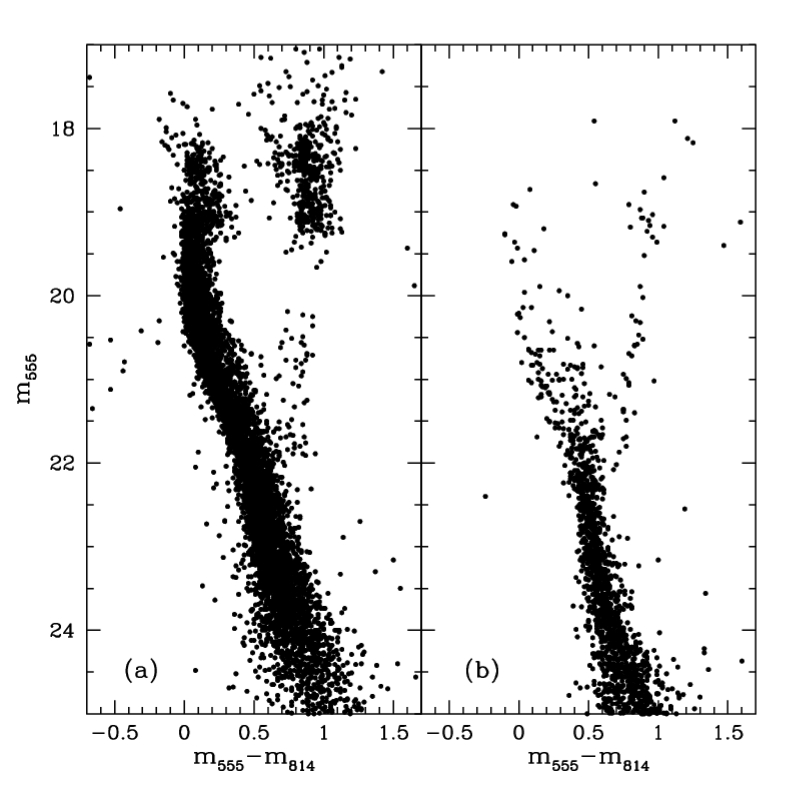
Figure 1: The on-cluster (a) and off-cluster (b) WFPC2 CMDs for NGC 1831. The former contains 7801 stars observed in the cluster’s direction while the latter has 2030 stars located in a field 7.3 arcmin away from the cluster’s centre.

2.1 Random photometric uncertainties

The random photometric uncertainties are the main source of spread in our HST/WFPC2 CMDs. Therefore, a suitable assessment of these uncertainties in both filters is crucial for correctly incorporating this effect into the artificial CMDs.

For the on-cluster field, two independent photometric measurements were available for a fraction of the stars due to the overlap region imaged by both the HALF and CEN fields (Santiago et al. 2001). Thus, we used the stars belonging to this overlap region to estimate the typical photometric uncertainties in the data. For each filter and at each magnitude bin, we estimated the dispersion, $\sigma^{\prime}$, in the distribution of differences between the independent magnitude measurements. For simplicity we assume that $\sigma^{\prime}$ is the composition of two equally-sized realizations of photometric error, $\sigma$. Thus, we get $\sigma^{\prime 2}=2\sigma^{2}$, and therefore

$$\sigma=\frac{\sigma^{\prime}}{\sqrt{2}}.$$

We emphasize that the two filters were treated as absolutely independent. As a consequence, the uncertainty in colour $m_{555}-m_{814}$, $\sigma_{\mathrm{colour}}$, will be the quadratic sum of the individual uncertainties:

$$\sigma_{\mathrm{colour}}^{2}=\sigma_{555}^{2}+\sigma_{814}^{2}.$$

Fig. 2 shows the derived uncertainties for MS stars in the two filters, $\sigma_{555}$ and $\sigma_{814}$, and for the colour, $\sigma_{\mathrm{colour}}$, using the expressions above.

For the off-clusters stars, we did not have two independent and overlapping WFPC2 images and, as a result, we could not apply the same method to quantify their photometric uncertainties. The solution found was to employ the same estimate as for the on-cluster stars. As the off-cluster image is deeper and sparser than the on-cluster ones, we can expect that this approximation yields an overestimate of the photometric uncertainties in the off-cluster data. However, the off-cluster CMD is used only for statistical subtraction of field contamination from the on-cluster CMD. We will see later that this particular correction technique is fairly independent of the estimated photometric uncertainties.

Figure 2: Estimated photometric uncertainties. Panel (a) shows the $\sigma_{555}$ (solid circles) and $\sigma_{814}$ (crosses) values as a function of apparent magnitude. Panel (b) shows the $\sigma_{\mathrm{colour}}$ calculated for the MS stars as a function of $m_{555}$.

2.2 Systematic photometric uncertainties

Systematic effects in WFPC2 data have been found by several authors. Johnson et al. (2001) measured an exposure time effect varying from 0.01 to 0.06 for different WFPC2 chips and filters in images of NGC 1805 and NGC 1818, as part of this project. de Grijs et al. (2002b) finds similar trends, but of slightly larger amplitude for the same data. Previously, Casertano & Muchtler (1998) found an exposure time effect but in the opposite sense as Johnson et al. (2001). Colour shifts of $\simeq 0.04$ have also been measured between different WFPC2 chips, possibly due to errors in CTE and aperture corrections or in zeropoints (see also Johnson et al. 1999).

Any photometric biases, as a function of either exposure time or chip, must be eliminated from our observed CMD, since the model CMDs which will be compared to it do not incorporate them.

As there does not seem to exist a consensus on the corrections to be applied, our approach was to empirically measure such biases and to apply appropriate shifts to the data when necessary. We searched for both exposure time and chip vs. chip effects. No systematic effects were found in the off cluster data. The main source of bias in the on-cluster data was found to be an offset between the PC and the Wide Field Camera (WFC) chips in the sense that MS stars with the same $m_{555}$ magnitude tend to be bluer by 0.05-0.10 mag when imaged with the PC than with the WFC. This applies to both HALF and CEN images. As the PC in the HALF image is centered on the cluster half-light radius, this effect is unlikely to be due to differences in crowding. In order to correct the data for this effect we first defined MS fiducial lines, taking the median $m_{555}-m_{814}$ colour at different magnitude bins. This was done separately for each chip and each image (CEN or HALF). We noticed that the WFC MS lines were more stable, always occupying loci in the CMD very close to each other. Thus, we transposed the PC fiducial lines to the corresponding WFC locus. The corrections are shown in Fig. 3. Panel (a) shows the uncorrected PC and WFC (a mean locus of the 3 chips) lines for both the CEN and HALF images. Panel (b) shows the corrected fiducial lines.

Figure 3: MS fiducial lines for each chip (PC or WFC) and image (CEN or HALF) as indicated: (a) original MS lines; (b) MS lines after applying the correction discussed in the text.

2.3 Selection effects

2.3.1 Sample incompleteness

Sample incompleteness occurs essentially due to two factors: overlapping of stellar profiles due to crowding and background noise. Therefore, in a cluster incompleteness will depend not only on apparent magnitude, but also on spatial position. Faint stars in dense stellar regions are the ones that suffer most from this effect. Completeness effects in the on-cluster data were previously discussed and measured by Santiago et al. (2001). These authors carried out experiments where artificial stars were added to the cluster image and subjected to the same sample selection as the real stars. The completeness c of each real star was estimated as the fraction of artificial stars of similar magnitude and location which were successfully recovered in the experiments. The estimated weight w for each star is then simply given by the inverse of its completeness ($w=1/c$). This weight corresponds to the total number of stars similar to the observed one which should be detected and measured in an ideal image.

Assigning a weight to each observed star is enough for the sake of luminosity and mass functions. However, correcting a CMD for incompleteness requires an extra step, namely to place an extra number of stars on the CMD according to the position of each observed star and its previously computed completeness weight. In order to fill the observed CMD with the missing stars, we first defined a fiducial line for the MS. As described in Sect. 2.2, this line was defined by taking the median $m_{555}-m_{814}$ colour at different magnitude bins. Given the $i^{th}$ MS star, its position along the fiducial line is provided by its $m_{555}$ magnitude and the corresponding $m_{555}-m_{814}$ colour. If its completeness weight is $w_{i}$, then $w_{i}-1$ extra stars were spread out from its position along the MS line taking the measured photometric uncertainties (as described in Sect. 2.1) into account. We assumed a Gaussian distribution of uncertainties both in $m_{555}$ magnitude and $m_{555}-m_{814}$ colour. Sample completeness falls to less than $50\%$ for $m_{555}\lower 2.15277pt\hbox{$\;\buildrel>\over{\sim}\;$}23.8$. We completed the CMD down to $m_{555}=24.5$ and then cut it at $m_{555}=23.5$, therefore avoiding boundary effects. A complete sample of stars both in number and in position resulted from this method.

As for the off-cluster CMD, it is complete at least down to $m_{555}=24.5$ (Castro et al. 2001).

2.3.2 Field star subtraction

Field star subtraction from the cluster sample is carried out in two separate steps. We first cut-off all stars in the on-cluster CMD which are much farther from the MS than expected by photometric errors. We therefore eliminate all evolved stars, as well as objects which are likely to be foreground stars or remaining non-stellar sources in the sample (distant galaxies, spurious image features, etc).

The second step involves the statistical removal of field stars located along the MS. We thus compare the distribution of stars in the on-cluster CMD to that of the off-cluster CMD. The comparison method is based on the hypothesis that the positions of the off-cluster stars represent the most likely positions for field stars on any similar CMD. We thus try to estimate the probability of each on-cluster star to be a field star and according to this probability we randomly remove stars from the on-cluster CMD.

We consider pairs of on-cluster/off-cluster stars. For each pair we compute the expected scatter in CMD position between the pair members under the assumption that they are independent photometric realizations of the off-cluster star. We will then have

$$\sigma_{\mathrm{c,555}}=\sqrt{2}\sigma_{\mathrm{off,555}}$$

and

$$\sigma_{\mathrm{c,colour}}=\sqrt{2}\sigma_{\mathrm{off,colour}}$$

respectively for the expected scatter in $m_{555}$ magnitude and $m_{555}-m_{814}$ colour, where the “off” subscript in the expressions above refers to the off-cluster pair member.

For the $i^{th}$ off-cluster CMD star we then consider the $N_{i}$ on-cluster stars inside a $3\sigma_{\mathrm{c,555}}$ x $3\sigma_{\mathrm{c,colour}}$ box centered on it. Using a Gaussian error distribution in magnitude and colour, we estimate the probability $p_{i,j}$ that the $j^{th}$ on-cluster CMD star, inside this box, is a second photometric measurement of the $i^{th}$ field star. Therefore,

$$p_{i,j}\propto exp{[\frac{-(mag_{i}-mag_{j})^{2}}{2(\sigma_{\mathrm{c,555}})^{2}}]}exp{[\frac{-(colour_{i}-colour_{j})^{2}}{2(\sigma_{\mathrm{c,colour}})^{2}}]}$$

where the normalization of $p_{i,j}$ is such that

$$\sum_{j=1}^{N_{i}}p_{i,j}=1$$

Doing the same for all $N_{\mathrm{off}}$ off-cluster CMD stars, we estimate the probability $P_{j}$ that the $j^{th}$ on-cluster CMD star is any one of the $N_{\mathrm{off}}$ field stars. Hence,

$$P_{j}=\sum_{i=1}^{N_{\mathrm{off}}}p_{i,j},$$

where

$$\sum_{j=1}^{N_{\mathrm{on}}}P_{j}=N_{\mathrm{off}}$$

and $N_{\mathrm{on}}$ is the total number of stars in the on-cluster CMD. In practice, not all off-cluster stars will have on-cluster stars within their $3\sigma_{\mathrm{c,555}}$ x $3\sigma_{\mathrm{c,colour}}$ boxes. The actual off-cluster stars taken into account will therefore be $N_{\mathrm{off}}^{\prime}<N_{\mathrm{off}}$.

Based on the $P_{j}$ probabilities, and scaling the number of field stars to the solid angle of the on-cluster field, we randomly remove

$$N_{\mathrm{field}}=N_{\mathrm{off}}^{\prime}\frac{\Omega_{\mathrm{on}}}{\Omega_{\mathrm{off}}}$$

stars from the on-cluster CMD, where $\Omega_{\mathrm{on}}$ and $\Omega_{\mathrm{off}}$ are the solid angles covered by the on-cluster and off-cluster fields, respectively.

Fig. 4 shows the results of correcting an observed NGC 1831 CMD for incompleteness and field contamination. Panel (a) shows the original CMD obtained from photometry, excluded of non-MS stars and corrected only for the systematic photometric effects described in Sect. 2.2. Panel (b) presents the complete CMD, i.e., corrected for sample incompleteness and cut at $m_{555}=23.5$; the extra stars added by completeness correction represent about 23% of the total within this magnitude range. Panel (c) shows the 89 stars ($\simeq$ 3%) in the on-cluster CMD that were considered as LMC field stars in the field star subtraction process; finally the clean and final cluster CMD is shown in panel (d).

We tested the field star subtraction algorithm for different box sizes and assumptions regarding the photometric scatter. The results are insensitive to the details in the algorithm.

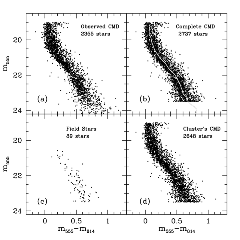
Figure 4: Correcting the on-cluster CMD for incompleteness and field stars contamination: (a) the observed CMD along the MS; (b) the CMD corrected for sample incompleteness and cut at $m_{555}$=23.5. The MS fiducial line for the cluster is shown in white ; (c) on-cluster stars considered as LMC field stars according to the algorithm described in the text; (d) final CMD with only stars presumed to belong to the cluster.

3 CMD modelling and statistical tools

3.1 CMD Modelling

We model the MS of a cluster as a single stellar population, characterized by stars of the same age and chemical composition. The first step is the choice of an isochrone, which defines a sequence of magnitude and colour as a function of mass for this population. For the present work we used Padova isochrones (Girardi et al. 2000) because they present masses inside the observed MS mass range ($M\lower 2.15277pt\hbox{$\;\buildrel<\over{\sim}\;$}2.5$ $M_{\odot}$) and are expressed in the vegamag WFPC2 photometric system. Notice that Padova models assume convective overshooting in the stellar interiors. This assumption may influence age determinations, specially when based in the position of turn-off and He-burning stars of younger populations (Testa et al. 1999, Barmina et al. 2002). However, as NGC 1831 is at least several Myr old and our modelling makes use of the entire MS, we believe that these model uncertainties tend to be of smaller importance in our analysis.

The free model parameters are: metallicity ($Z$), age ($\log(\tau)$), intrinsic distance modulus $(m-M)_{0}$, reddening (E(B-V)), PDMF slope ($\alpha=-\mathrm{d}\log\Phi(M)/\mathrm{d}\log M$) and unresolved binary fraction ($f_{\mathrm{bin}}$). The PDMF was considered as a power-law ($\Phi(M)=\Phi_{0}M^{-\alpha}=\mathrm{d}N/\mathrm{d}M$), where the only free parameter is the slope $\alpha$. $f_{\mathrm{bin}}$ is defined as the systemic binary fraction, $f_{\mathrm{bin}}=N_{\mathrm{bin}}/(N_{\mathrm{bin}}+N_{\mathrm{sing}})$, where $N_{\mathrm{bin}}$ and $N_{\mathrm{sing}}$ are, respectively, the number of unresolved pairs and single stars.

The process of generating artificial stars works as follows:

(1) we fix $Z$ and $\log(\tau)$ for the stellar population by means of a chosen isochrone;

(2) we randomly draw a stellar mass according to the PDMF and get the absolute magnitudes in the two desired filters through the mass-luminosity relation given by the isochrone;

(3) for $f_{\mathrm{bin}}$ randomly chosen cases, we repeat step (2), representing a companion star in a binary system, and combine the two luminosities in both filters;

(4) we apply the intrinsic distance modulus $(m-M)_{0}$ and reddening vector($A_{\mathrm{V}},E(B-V)$) to the system, defining its theoretical CMD position. For this purpose, we use $R_{\mathrm{V}}=A_{\mathrm{V}}/E(B-V)=3.1$ and the photometric transformation to the vegamag WFPC2 system according to Holtzman et al. 1995a;

(5) we introduce the photometric uncertainties by spreading the star with a Gaussian distribution of errors with $\sigma_{555}$ and $\sigma_{814}$ as empirically determined (see Sect. 2.1). This yields observational versions of the magnitude and colour;

(6) finally, we verify if the star is inside the MS observational ranges in magnitude and colour defined for the data and throw it away if it is not.

For each model realization we generate the same number of MS stars as observed in the real CMD, corrected for sample incompleteness and field contamination, and located inside the $19.0\leq m_{555}\leq 23.5$ range. This range in apparent magnitude corresponds to $0.5\lower 2.15277pt\hbox{$\;\buildrel<\over{\sim}\;$}M_{555}\lower 2.15277pt\hbox{$\;\buildrel<\over{\sim}\;$}5.0$ and $0.9\lower 2.15277pt\hbox{$\;\buildrel<\over{\sim}\;$}M\lower 2.15277pt\hbox{$\;\buildrel<\over{\sim}\;$}2.3$ $M_{\odot}$.

The best models are chosen by a direct comparison of the observed CMD with the artificial ones. The statistical tools used in this comparison are presented in the next section. The model vs. observation comparison strategy is as follows:

(1) the global parameters for the cluster, $\log(\tau)$, $Z$, $E(B-V)$ and $(m-M)_{0}$, are determined using the CMD of the central cluster region ($R\leq 30$ arcsec, where $R$ is the projected distance from the cluster’s centre), where field contamination and statistical noise are minimized (see Table 1);

(2) for the best combinations of the global parameters, the position dependent parameters $\alpha$ and $f_{\mathrm{bin}}$ are then derived using the CMDs in concentric rings of variable radii.

Table 1 shows important information about the cluster regions used in this modelling process. The first column gives the range in $R$, Col. (2) the original number of CMD stars in the $19.0\leq m_{555}\leq 23.5$ range, Col. (3) the number of stars in the completeness corrected CMD (see Sect. 2.3.1), Col. (4) the number of assigned field stars (Sect. 2.3.2) and, finally, Col. (5) the number of stars in the CMD used in the modelling process. Notice that, not unexpectedly, field contamination becomes a serious issue for the outermost region, since statistical removal of field stars reduces the CMD numbers by about 40%. On the other hand, crowding in the central regions yields larger photometric incompleteness, as reflected by the clear increase in the number of stars between Cols. (2) and (3).

This modelling strategy allows an efficient and systematic search of best fit models in a 6-dimensional parameter space and makes use of the 2-dimensional information provided by the CMD data. Furthermore, this strategy naturally splits the parameters into those that define the position of the MS in the CMD plane (the global ones) and those that influence the way stars are distributed within the MS locus (the position dependent ones).

Fig. 5 shows four CMDs for the central cluster region. The one in the bottom right (panel d) is the real data, whereas the other three are realizations from different models generated by the modelling process described above. The input model parameters are shown in each panel. The three model CMDs do in fact look different, their MS ridge lines having different shapes and occupying different positions along the CMD plane.

Table 1: Number of points in the different cluster regions whose CMDs are used in the CMD modelling as described in Sect. 3.1.

Region (arcsec)	observed	complete	field stars	cluster
$0<R\leq 30$	2221	2737	89	2648
$0<R\leq 15$	1220	1506	27	1479
$15<R\leq 30$	1001	1216	62	1154
$30<R\leq 60$	1692	1972	240	1732
$R>60$	1673	1780	765	1015

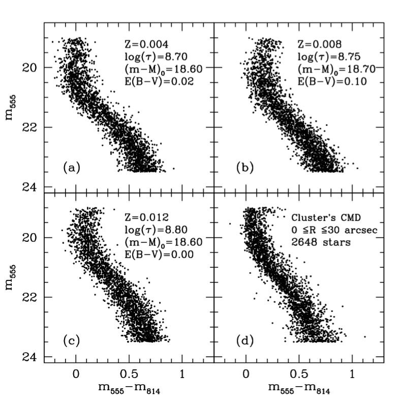
Figure 5: CMDs for the cluster central region: panels a, b and c show realizations from the modelling process while panel d shows the result of the real data treatment (Sect. 2). The input model parameters are indicated in each panel, where $\alpha=2.30$ and $f_{\mathrm{bin}}=0.30$ for all models.

3.2 Statistical tools

One of the main goals of this paper is to establish an objective comparison method between models and data. This required developing and applying statistical criteria that discriminate the model CMDs that most adequately reproduce the observed one. Ideally these comparison criteria should be both simple and easy to implement but yet make use of as much information provided by the bidimensional colour-magnitude plane as possible. We stress that these methods, in principle, are not restricted only to CMD analyses, but may be applied to the comparison of any two bidimensional distributions of points. In similar context as in this work, statistical techniques of CMDs comparison have been successfully applied by Kerber et al. (2001), Lastennet & Valls-Gabaud (1999), Saha (1998), Hernandez et al. (1999), allowing a model reconstruction of the main CMD features displayed by the component stars within a galaxy or a cluster.

Three statistics of CMD comparison were considered in this paper: $S^{2}$, $PSS$ and $L$. The first two are explained in more detail by Kerber et al. (2001). $S^{2}$ is essentially a dispersion between model and data points in the CMD plane; $PSS$ is proportional to the joint probability that the two CMDs being compared are drawn from the same population.

As for the $L$ statistics, it is an empirical version of the likelihood statistics described and used by Hernandez et al. (1999). For each model, 300 realizations with the same number of artificial stars as the real data (hereafter $N_{\mathrm{obs}}$) were generated. Dividing the CMD plane into $N_{\mathrm{b}}$ boxes, the model probability of one star, randomly chosen from any of these 300 realizations, to be inside the $k^{th}$ box is given by $p_{k}=N_{k}/(300\leavevmode\nobreak\ N_{\mathrm{obs}})$. $N_{k}$ is the sum of stars from all realizations which fall in the $k^{th}$ box. Thus, $p_{k}$ may be interpreted as a probability function along the CMD plane.

The likelihood L of a given model is then defined as

$$L=\prod_{i=1}^{N_{\mathrm{obs}}}p_{\mathrm{obs},i}$$

or

$$\log L=\sum_{i=1}^{N_{\mathrm{obs}}}\log(p_{\mathrm{obs},i}),$$

where the product and sum are over the $N_{\mathrm{obs}}$ observed stars, and $p_{\mathrm{obs},i}$ is the model probability function evaluated at the CMD position of the $i^{th}$ observed star.

So, for each model we have three distinct statistical values. In order to establish the best models we build diagnostic diagrams (hereafter DDs), which are planes where we confront any two of these statistics. The best models will naturally have large $L$ and $PSS$, and small $S^{2}$ values. The method was tested by means of control experiments, that are shown in Sect. 4.

3.3 The model grids

The model input values for $\log(\tau)$, $Z$, $(m-M)_{0}$, $E(B-V)$ were chosen in order to bracket those found in the literature. In this respect, the web page www.ast.cam.ac.uk/STELLARPOPS/LMCdatabase by Richard de Grijs was very useful as it includes a very large compilation of parameter values and references on the 8 LMC rich clusters imaged by the GO7307 project.

In accordance with this database, we set the range of possible values for each physical parameter and created a regular model grid within this range. We expect this systematic grid to prevent biases in the parameter values determination.

Using the cluster central region ($0\leq R\leq 30$ arcsec), we explored the following space defined by the global parameters:

$Z=0.004,0.008,0.012$

$\log(\tau/\mathrm{yr})=8.70,8.75,8.80$

$(m-M)_{0}=18.30,18.40,18.50,18.60,18.70$

$E(B-V)=0.00,0.02,0.04,0.06,0.08,0.10$

The position dependent parameters were kept fixed as $\alpha=2.30$ and $f_{\mathrm{bin}}=0.30$. Therefore this initial grid has 270 models.

Once the CMD comparison statistics defined in Sect. 3.2 are computed for each model, the DDs are built and the best models are identified, we investigate the dynamically affected, position dependent parameters by generating artificial CMDs to be compared to the observed CMDs within the concentric rings. In this second step we explored the following bidimensional parameter space:

$\alpha=1.40,1.70,2.00,2.30,2.60$

$f_{\mathrm{bin}}=0.25,0.50,0.75$

A total of 180 models were built for each ring, the only difference between one ring and another being the number of artificial stars.

4 Control Experiments

As mentioned in Sect. 3.2, we tested the validity of our statistical methods using control experiments. These experiments consist of drawing one realization of some specific model and calling it the “observed CMD”. We then verify if the DDs recover the generating model (hereafter input model) as the best one describing the “observed CMD”.

Figs. 6 and 7 show the results of a control experiment involving the 270 models to be latter applied to the NGC 1831 central region. All panels show DDs of $\log S^{2}$ vs. $\log L$, each point in the DD representing a particular model. The panels on the right are blow-ups of those on the left, showing in detail the region where the best models are located; this region corresponds to larger $\log L$ and smaller $\log S^{2}$ values. The different symbols in a single panel are coded according to the values of one of the four global model parameters ($Z$, $\log(\tau)$, $(m-M)_{0}$ and $E(B-V)$), therefore allowing the effect of varying each parameter to be separately assessed. Notice that the figures do not show the entire model grid in order to avoid cluttering. The grid regions discarded from the DDs are those of systematically high $\log S^{2}$ and low $\log L$ values. The “observed CMD” was taken to be a realization of the model with $Z=0.008$, $\log(\tau)=8.75$, $(m-M)_{0}=18.50$ and $E(B-V)=0.06$. This input model is shown as the large star in the blowup panels.

A tight correlation between the two statistics is clearly seen in all panels, adding reliability and stability to the choice of the best fitting models. The control experiments also show that one is in fact capable of recovering the input model based on the values of the statistics used: it is the model with largest $\log L$ and smallest $\log S^{2}$, as ideally we would expect.

Another important result from Figs. 6 and 7 is the combining and/or canceling effect of some global parameters, yielding models of comparable quality. As an example, the effects of metallicity $Z$ and reddening $E(B-V)$ tend to cancel each other. Some models with $Z$ ($E(B-V)$) lower (higher) than the input value, along with some high $Z$ and low $E(B-V)$ ones, rank among the best models in the DDs. This degeneracy in the DDs is not surprising since the effect of increasing $Z$ is to make stars redder and fainter at a given mass, roughly opposite to the effect of decreasing $E(B-V)$.

Figure 6: DDs resulting from the control experiment for the cluster’s central region, showing the effects of varying metallicity (panels (a) and (b)) and age (panels (c) and (d)). The symbols are as indicated in the panels on the left. The panels on the right show the best models in detail and use the same symbol notation.

Figure 7: DDs resulting from the control experiment for the cluster’s central region, showing the effects of varying distance (panels (a) and (b)) and reddening (panels (c) and (d)). The symbols are as indicated in the panels on the left. The panels on the right show the best models in detail.

Fig. 8 presents similar DDs as in Figs. 6 and 7, but shows the model grid to be applied to the concentric regions of NGC 1831 (in a total of 180 models). The symbols now indicate different values of the PDMF slope $\alpha$ (panels (a) and (b)) and binary fraction $f_{\mathrm{bin}}$ (panels (c) and (d)). As before, the panels on the right are blow-ups of the ones on the left, showing the best models only. The input model (large star), in this case, is the one with $\alpha=2.00$, $f_{\mathrm{bin}}=0.50$ (and $Z=0.012$, $\log(\tau)=8.75$, $(m-M)_{0}=18.60$, $E(B-V)=0.02$). It is again located at the extreme upper left corner of the DD, confirming the applicability of our statistical approach.

However, the panels on the right show that the three best models have the same $\alpha$ ($=2.00$) but different $f_{\mathrm{bin}}$ values, revealing a larger difficulty in determining the latter than the former. This occurs because the effect caused by binaries is of the same order as or smaller than the photometric uncertainties in our WFPC2 CMDs. Consequently, as will be discussed in Sect. 5.2, the $f_{\mathrm{bin}}$ determination by means of our CMDs becomes a difficult task.

Notice that, in comparison with the DDs for the central region, the DDs in Fig. 8 present a larger dispersion. This is caused by the much smaller number of stars used in the set of models with varying $\alpha$ and $f_{\mathrm{bin}}$; in this case, all model CMDs (including the “observed” one) have 1154 stars, therefore mimicking the situation of the second concentric region to be studied in NGC 1831 (see Table 1).

Figure 8: DDs resulting from the control experiment for the $15\leq R\leq 30$ arcsec region. Panels (a) and (b) (the latter is a blowup of the former) show the effect of varying PDMF slope $\alpha$, whereas panels (c) and (d) (the latter is a blowup of the former) show the effect of varying $f_{\mathrm{bin}}$. The input model is represented by the large star.

Fig. 9 shows DDs involving the $PSS$ statistics. The upper panels show $PSS$ vs. $\log L$ and $PSS$ vs. $\log S^{2}$ plots for the central region. The lower panels show the same plots for one of the concentric rings. The same models as in Figs. 6, 7, and 8 are depicted but without symbol coding as a function of parameter values. The correlation between $PSS$ and the other statistics is again quite tight. In fact, the results based on the DDs are insensitive to the particular choice of statistics to be plotted. This is a very important result, since it further enhances the reliability of our statistical CMD modelling techniques. For the sake of simplicity, we hereafter restrict ourselves to $\log L$ vs. $\log S^{2}$ DDs only.

Figure 9: DDs involving the PSS statistics in control experiments. The upper (lower) panels show $PSS$ vs. $\log L$ and $PSS$ vs. $\log S^{2}$ plots for the region inside $0\leq R\leq 30$ ($15<R\leq 30$) arcsec.

5 Results

5.1 Central region

In this section we model the CMD of stars belonging to the region within $R\leq 30$ arcsec from the centre of NGC 1831. In accordance with Santiago et al. (2001), this corresponds roughly to $R\lower 2.15277pt\hbox{$\;\buildrel<\over{\sim}\;$}7$ pc or within 2 half-light radii. As indicated in Table 1, there are 2221 stars in this region in the magnitude range $19.0\leq m_{555}\leq 23.5$. As also mentioned earlier, this central cluster region suffers from insignificant contamination by LMC field stars. On the other hand, due the high stellar density, incompleteness effects become more important. The chosen faint magnitude cut-off represents the magnitude at which completeness falls at $50\%$, in an attempt to reduce the relevance of this effect on our results.

The DDs for the model vs. real CMD comparison are presented in Figs. 10 and 11. As in the control experiments, the correlation between $\log L$ and $\log S^{2}$ is quite noticeable, the best models being again at the upper left region in the panels. These figures follow the same conventions and notations as Figs. 6 and 7, therefore allowing us to assess the effect of varying each global cluster parameter separately. For example, panels 10(a) and 10(b) clearly show that the best models have $Z=0.012$. The effects of the other parameters are not as striking as in the case of metallicity. Yet, panels 10(c) and 10(d) favour an age in the range $8.75\leq\log(\tau)\leq 8.80$. Likewise, the three lowest values of intrinsic distance modulus (two of which are not even shown in the figure) can essentially be ruled out (panels 11(a) and 11(b)), placing NGC 1831 near or beyond the distance to the LMC centre. Finally, $E(B-V)\leq 0.02$ is favoured by our modelling approach (panels 11(c) and 11(d)). Notice that this latter parameter is again anti-correlated with $Z$, in the sense that the models in the blowup panels with $Z=0.008$ (circles in panel 10(b)) have larger $E(B-V)$ values (circles or crosses in panel 11(d)).

These best choices of the global parameters, as discussed in Sect. 3.1, besides being useful constraints by themselves, serve as model inputs to the position dependent parameters $\alpha$ and $f_{\mathrm{bin}}$, whose modelling is based on the concentric regions.

Figure 10: DDs resulting from the CMD of the cluster’s central region, showing the effects of varying metallicity (panels (a) and (b)) and age (panels (c) and (d)). The symbols are as indicated in the panels on the left. The panels on the right show the best models in detail.

Figure 11: DDs resulting from the CMD of the cluster’s central region, showing the effects of varying distance (panels (a) and (b)) and reddening (panels (c) and (d)). The symbols are as indicated in the panels on the left. The panels on the right show the best models in detail.

5.2 Concentric regions

We now analyze the NGC 1831 CMDs in the concentric regions listed in Table 1. As just mentioned, the free model parameters in this case are the PDMF slope $\alpha$ and the unresolved binary fraction $f_{\mathrm{bin}}$. For all regions we corrected the observed CMD to the effects of sample incompleteness and field star contamination. Fig. 12 shows their final CMDs. As mentioned before, Table 1 shows the number of points in all the steps along the data correction process.

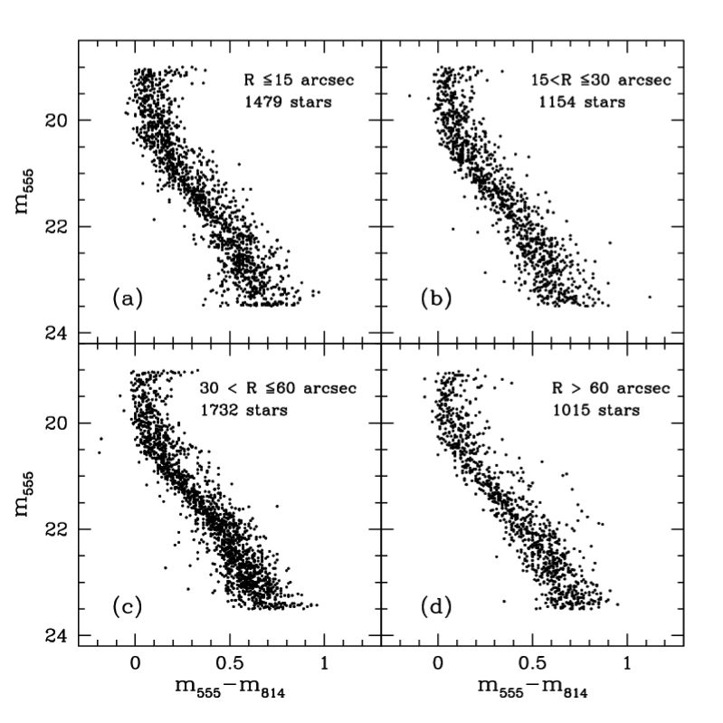
Figure 12: The final NGC 1831 CMDs in four concentric regions: (a) $0<R\leq 15$ arcsec; (b) $15<R\leq 30$ arcsec;(c) $30<R\leq 60$ arcsec;(d) $R>60$ arcsec.

In the modelling, we apply the same model grid for every region, only changing the number of artificial stars generated. The results from the previous section were used to restrict the possible values of the cluster s global parameters, allowing us to investigate the dynamically dependent parameters for the system.

Figs. 13 and 14 present the DDs resulting from model vs. data CMD comparison in the four regions. The different symbols in each panel correspond to different values of $\alpha$. As usual, the panels on the right show the best models in detail. The results for the two innermost regions are presented in Fig. 13. Panels (a) and (b) indicate that the best models for innermost region ($R\leq 15$ arcsec) have $1.40\leq\alpha\leq 1.70$. In the ring $15<R\leq 30$ arcsec, shown in panels (c) and (d) of the same figure, the best models present similar $\alpha$ values: $1.40\leq\alpha\lower 2.15277pt\hbox{$\;\buildrel<\over{\sim}\;$}1.70$.

In Fig. 14 we have the results for the two outermost rings. Panels (a) and (b) show the DDs for the stars with $30<R\leq 60$ arcsec. Now, there is evidence for a sharp change in the PDMF s slope: the best models have $2.30\leq\alpha\leq 2.60$. Finally, the DD for the most peripheric ring has a large dispersion (panels 14(c) and 14(d) ). This spread is also seen in the best PDMF slope: values in the range $2.00\lower 2.15277pt\hbox{$\;\buildrel<\over{\sim}\;$}\alpha\leq 2.60$ are seen in the upper left corner of the DD. This may reflect large uncertainties in the field star subtraction, since it leads to a large reduction of CMD points in this ring.

For each ring, we assign a representative $\alpha$ and associated uncertainty using the 10 models with the largest values of likelihood $L$. The final slope is taken to be the weighted average value among these best models, and its associated uncertainty is the dispersion around the average. The weight assigned to each model was the inverse of the difference in $\log L$ between the observed CMD and a CMD from a typical model realization. This difference is a measure of the discrepancy between model and observed CMDs. Table 2 lists the final $\alpha$ values and uncertainties for each ring (Cols. 3 and 4). The first 2 columns in the table show the regions in arcsec and parsecs (assuming $(m-M)_{0}=18.61$ for NGC 1831 as adopted in Sect. 6), respectively.

Table 2: Best estimates of the slope $\alpha$ and its uncertainty as a function of distance to the centre.

Region (arcsec)	Region (pc)	$\alpha$	$\sigma_{\alpha}$
$0<R\leq 15$	$0<R\leq 3.8$	1.72	0.15
$15<R\leq 30$	$3.8<R\leq 7.6$	1.68	0.19
$30<R\leq 60$	$7.6<R\leq 15.2$	2.45	0.15
$R>60$	$R>15.2$	2.19	0.33

As for the fraction of unresolved binaries, $f_{\mathrm{bin}}$, the results, as anticipated, are not conclusive in any ring, given the CMD spread. A more precise treatment of photometric errors may help constrain this parameter.

Figure 13: DDs resulting from the CMDs of concentric regions, showing the effect of varying $\alpha$. The upper (lower) panels show the results for stars in the region with $0\leq R\leq 15$ ($15<R\leq 30$) arcsec. The panels on the left show the entire DD, while those on the right show the best models in detail. The symbols are as indicated in the panels on the right.

Figure 14: DDs resulting from the CMDs of concentric regions, showing the effect of varying $\alpha$. The upper (lower) panels show the results for stars in the region with $30<R\leq 60$ ($R>60$) arcsec. The panels on the left show the entire DD, while those on the right show the best models in detail. The symbols are as indicated in the panels on the right.

6 Summary and Conclusions

In this work we analyzed a deep CMD of NGC 1831, a rich LMC cluster, obtained from HST/WFPC2 images in the F555W and F814W filters. We inferred physical parameters such as metallicity, age, intrinsic distance modulus, reddening and PDMF slopes by comparing the cluster CMD with artificial ones. We presented in detail the techniques used to build the model CMDs, which use these parameters as model input and take into account observational uncertainties as in the real data. The parameter space explored by our regular model grids bracketed the values found in the literature.

The model vs. data comparison required correcting the observed CMD for selection effects caused by photometric incompleteness and CMD contamination by stars belonging to the LMC field. We also presented the statistical techniques used to compare the real CMD, corrected for the aforementioned selection effects, to the artificial ones. These statistical tools allowed us to discriminate the models that best reproduce the data. They are based on simple and objective statistical quantities and make use of the full bidimensional distribution of points in the CMD.

The best parameter values inferred for NGC 1831 are in the ranges $8.75\leq\log(\tau)\leq 8.80$, $18.50\leq(m-M)_{0}\leq 18.70$, $0.00\leq E(B-V)\leq 0.02$. Using the weighted average value among the 10 best models, as described in Sect. 5.2, we have $\tau=588\pm 43$ Myr, $(m-M)_{0}=18.61\pm 0.07$, $E(B-V)=0.013\pm 0.015$. As for the metallicity, all 10 best models have $Z=0.012$.

As discussed in Sect. 4, there is a coupling between reddening and metallicity, and therefore the determination of the former limits the values of the latter. As a consequence, the derived high metallicity for NGC 1831 brings about a low reddening determination.

The combined values of the global parameters obtained in this work for NGC 1831 suggest that this cluster is: a) metal-richer and older than in most previous estimates; b) placed near or beyond the distance to the LMC centre; c) found in a low reddening region.

Our estimated age and metallicity for NGC 1831 are in perfect accordance with the age-metallicity relation for LMC clusters obtained by Olszewski et al. (1991).

The best models for the global parameters were then used to build artificial CMDs of regions separated according to distance from the cluster centre and with varying values of the PDMF slope and fraction of unresolved binaries. For the PDMF slope $\alpha$ our statistical modelling shows that significant mass segregation exists in NGC 1831: for the central regions (out to 30 arcsec $\simeq 7.6$ pc), we derive $\alpha\simeq 1.70$, whereas $\alpha\lower 2.15277pt\hbox{$\;\buildrel>\over{\sim}\;$}2.20$ for the outer regions. As for binarism, our results were not as conclusive. One explanation is that the spread in the CMD caused by unresolved binaries is of similar or smaller amplitude than the empirically derived photometric uncertainties in the data. Therefore, this parameter is highly sensitive to the adopted photometric errors, rendering its realistic estimate a task for yet deeper CMDs or for data for which photometric uncertainties may be better estimated and modelled.

In a preliminary analysis of these data, Santiago et al. (2001) observed the effect of mass segregation in NGC 1831 with a steepening of the LF slope as a function of distance from the centre. However, no PDMF was derived. A global PDMF slope for NGC 1831 is presented by Mateo (1988), through the conversion of the luminosity function down to $V\sim 23$ ($M\lower 2.15277pt\hbox{$\;\buildrel>\over{\sim}\;$}\mbox{$M_{\odot}$}$) into a PDMF. The resulting slope is $\alpha\sim 4.0$, therefore considerably steeper than our position dependent ones. Global slope values of other clusters from Mateo (1988) are in the range $2.5\lower 2.15277pt\hbox{$\;\buildrel<\over{\sim}\;$}\alpha\lower 2.15277pt\hbox{$\;\buildrel<\over{\sim}\;$}4.6$. In contrast, Elson et al. (1989) find much shallower slopes $0.8\lower 2.15277pt\hbox{$\;\buildrel<\over{\sim}\;$}\alpha\lower 2.15277pt\hbox{$\;\buildrel<\over{\sim}\;$}1.8$ for another sample of rich LMC clusters. These earlier results are based on ground-based observations, for which the effects of crowding are much more serious than in the present work.

Our determined position dependent PDMFs constrain the $\alpha$ values within $\sim 0.2$. These results can be used along with N-body simulations in order to recover the initial conditions, in particular the cluster IMF. We are applying the techniques shown in this paper to the others LMC clusters imaged with HST/WFPC2 as part of the GO7307 project in order to infer the same physical information as for NGC 1831. These future results can be very useful in investigations on the IMF universality.

- (1) Baraffe, I., Chabrier, G., Allard, F., & Hauschildt, P. 1998, A&A, 337, 403
- (2) Barmina, R., Girardi, L., & Chiosi, C. 2002, A&A, 285, 847
- (3) Beaulieu, S., Elson, R., Gilmore, G., et al. 1999, New Views of the Magellanic Clouds, IAU Symp. 190, Y.-H. Chu, N. Suntzeff, J. Hesser, & D. Bohlender, 460
- (4) Beaulieu, S., Gilmore, G., Elson, R., et al. 2001, AJ, 121, 2618
- (5) Bica, E., Dottori, H., & Pastoriza, M. 1986, A&A, 156, 261
- (6) Brocato, E., Di Carlo, E., & Menna, G. 2001, A&A, 374, 523
- (7) Casertano, S., & Muchtler, M. 1998, WFPC2 Instrument Science Report 98-02
- (8) Castro, R., Santiago, B., Gilmore, G., Beaulieu, S., & Johnson, R. 2001, MNRAS, 326, 333
- (9) Corsi, C., Buonanno, R., Fusi Pecci, F., et al. 1994, MNRAS, 271, 385
- (10) Chiosi, C. 1989, RMxAA, 18, 125
- (11) Cowley, A. P., & Hartwick, F. D. A. 1992, PASP, 104, 1216
- (12) de Grijs, R., Johnson, R., Gilmore, G., & Frayn, C. 2002b, MNRAS, 331, 228
- (13) de Grijs, R., Gilmore, G., Johnson, R. & Mackey, A. D. 2002a, MNRAS, 331, 245
- (14) De Marchi, G., & Paresce, F. 1995, A&A, 304, 211
- (15) de Oliveira, M. R., Bica, E., & Dottori, H. 2000, MNRAS, 311, 589
- (16) Elson, R., Fall, S. M., & Freeman, K. C. 1987, ApJ, 323, 54
- (17) Elson, R., Fall, S. M., & Freeman, K. C. 1989, ApJ, 336, 734
- (18) Elson, R., Gilmore, G., Santiago, B., & Casertano, S. 1995, AJ, 110, 682
- (19) Gallart, C., Aparicio, A., Bertelli, G., & Chiosi, C. 1996, AJ, 112, 1950
- (20) Gallart, C., Freedman, W. L., Aparicio, A., Bertelli, G., & Chiosi, C. 1999, AJ, 118, 2245
- (21) Girardi, L., Chiosi, C., Bertelli, G., & Bressan A. 1995, A&A, 298, 87
- (22) Girardi, L., Bressan, A., Bertelli, G., & Chiosi, C. 2000, A&AS, 141, 371
- (23) Goodwin, S. P. 1997, MNRAS, 286, 669
- (24) Heggie, D., & Aarseth, S. 1992, MNRAS, 257, 513
- (25) Hernandez, X., Valls-Gabaud, D., & Gilmore G. 1999. MNRAS, 304, 705
- (26) Hernandez, X., Gilmore, G., & Valls-Gabaud D. 2000, MNRAS, 317, 831
- (27) Holtzman, J., Hester, J., Casertano, S., et al. 1995a, PASP, 107, 156
- (28) Holtzman, J., Gallagher, J., Cole, A., et al. 1999, AJ, 118, 2262
- (29) Johnson, J., Bolte, M., Stetson, P., Hesser, J., & Sommerville, R. 1999, ApJ, 527, 199
- (30) Johnson, R., Beaulieu, S., Gilmore, G., et al. 2001, MNRAS, 324, 367
- (31) Kerber, L., Javiel, S., & Santiago, B. 2001, A&A, 365, 424
- (32) Kroupa, P. 2001, MNRAS, 322, 231
- (33) Kroupa, P., Aarseth, S., & Hurley, J. 2001, MNRAS, 321, 699
- (34) Lastennet, E., & Valls-Gabaud, D. 1999, RMxA Conf. Ser., 8, 115
- (35) Mateo, M. 1987, ApJ, 323, L41
- (36) Mateo, M. 1988, ApJ, 331, 261
- (37) Meurer G. R., Cacciari C., & Freeman K. C. 1990, AJ, 99, 1124
- (38) Olszewski, E. W., Schommer, R. A., Suntzeff, N. B, & Harris, H. C. 1991, AJ, 101, 515
- (39) Panagia, N., Gilmozzi, R., Macchetto, F., Adorf, H.-M., & Kirshner, R. 1991, ApJ Letters, 380, L23
- (40) Piotto, G., Cool, A., & King, I. 1997, AJ, 113, 1345
- (41) Saha, P. 1998, AJ, 115, 1206
- (42) Santiago, B., Elson, R., & Gilmore G. 1996, MNRAS, 281, 1363
- (43) Santiago, B., Beaulieu, S., Johnson, R., & Gilmore, G. 2001, A&A, 369, 74
- (44) Spurzem, R., & Aarseth, S. 1996, MNRAS, 282, 19
- (45) esta, V., Ferraro, F., Chieffi, A., et al. 1999, AJ, 118, 2864
- (46) Vallenari, A., Chiosi, C., Bertelli, G., Meylan, G., & Ortolani, S. 1992, AJ, 104, 1100
- (47) Vesperini, E., & Heggie, D. 1997, MNRAS, 289, 898
- (48) Westerlund, B. E. 1990, A&AR, 2, 29