STJ Observations of the Eclipsing Polar HU Aqr

Abstract

We apply an eclipse mapping technique to observations of the eclipsing magnetic cataclysmic variable HU Aqr. The observations were made with the S-Cam2 Superconducting Tunnel Junction detector at the WHT in October 2000, providing high signal-to-noise observations with simultaneous spectral and temporal resolution. HU Aqr was in a bright (high accretion) state ($V=14.7$) and the stream contributes as much to the overall system brightness as the accretion region on the white dwarf. The stream is modelled assuming accretion is occuring onto only one pole of the white dwarf. We find enhanced brightness towards the accretion region from irradiation and interpret enhanced brightness in the threading region, where the ballistic stream is redirected to follow the magnetic field lines of the white dwarf, as magnetic heating from the stream$\--$field interaction, which is consistent with recent theoretical results. Changes in the stream eclipse profile over one orbital period indicate that the magnetic heating process is unstable.

Figure 1: White light curves and sky-backgrounds for cycle 29982 (upper plot), 29994 (middle plot) and 29995 (lower plot). The background is taken from pixels (1,1) and (6,6), while the light curves are from all 36 pixels. The light curves are in 1 s time bins (0.00013 phase) and the backgrounds in 18 s time bins to facilitate direct comparison. The abscissa scales have been adjusted so the eclipses lie at the same locations. A neutral density filter was used for cycle 29994, hence the lower count rate and increased noise, and the seeing was poor for the first part of cycle 29982.

1 Introduction

HU Aqr is a member of the AM Her sub-class of cataclysmic variables, also called polars because of their highly polarised optical emission. Polars are characterised by a white dwarf primary with a strong magnetic field ($\sim 10-240$ MG) and no accretion disc (see Cropper 1990 and Warner 1995 for reviews). The secondary is a main sequence star which fills its Roche lobe, resulting in an overflow of material from the inner Lagrangian point to form an accretion stream. The stream is initially on a ballistic freefall trajectory, until at some radius the magnetic pressure of the white dwarf magnetic field is approximately equal to the ram pressure of the stream. At this point the stream is threaded onto the field lines of the white dwarf and accretes onto a small area near one or both of the magnetic poles.

HU Aqr is an eclipsing polar with a period of $\sim$ $125$ mins, lying just below the period gap (see e.g. Howell, Nelson & Rappaport 2001). Harrop-Allin, Hakala & Cropper (1999b) used the eclipse of the white dwarf primary by the secondary to establish the distribution of brightness along the stream given a number of parameters defining both the geometry of the system and the physical parameters of the model. The stream emission was calculated using model light curves which are optimized by a genetic algorithm, based on a method first employed on photometric eclipse profiles of HU Aqr by Hakala (1995). The technique was developed and improved by Harrop-Allin et al. (1999a) and applied to observations of HU Aqr in both a high and low accretion state (high- and low-mass transfer; Harrop-Allin et al. 1999b and Harrop-Allin, Potter & Cropper 2001).

This method of eclipse mapping has also been applied to emission-lines (Sohl & Wynn 1999; Vrielmann & Schwope 2001; Kube, Gänsicke and Beurmann 2000). Kube et al. (2000) used HST FOS spectra of (another polar) UZ For to map the accretion stream line emission at Civ $\lambda$ 1550Å, and Vrielmann & Schwope (2001) used the emission line light curves of H$\beta$, H$\gamma$ and He ii $\lambda$4686Å of HU Aqr. Both these line-emission methods use a three-dimensional stream so data from the entire orbit of the system is fitted and the model can reproduce the out-of-eclipse features, such as the pre-eclipse dips (Watson 1995). They can also reproduce the effect of differing brightness distributions between the irradiated and un-irradiated faces of the stream, and this effect is not reproduced in the model of Harrop-Allin et al. (1999a and 1999b). However, the Harrop-Allin et al. technique has the benefit of being sensitive to the total emission from the stream (not just the line emission). The technique also has the advantage of access to high signal-to-noise ratio data, which is crucial in producing robust fits.

The light curves presented here were obtained using the S-Cam2 Superconducting Tunnel Junction (STJ) camera, developed by the ESA Astrophysics Division at ESTEC. The camera is the second prototype of a new generation of detectors that record the energy as well as the position and time of arrival (to within $\sim 5\ \mu$s for this particular detector) of the incident photons (Rando et al. 2000). The application of STJs to optical photon counting was first proposed by Perryman, Foden & Peacock (1993), and has since been applied to observations of the Crab Pulsar (Perryman et al. 1999), the magnetic cataclysmic variable UZ For (Perryman et al. 2001) and to quasar spectroscopy (de Bruijne et al. 2002).

The detector itself consists of a liquid helium cooled array of $6\times 6$ pixels, each being $25\times 25$ $\mu$m², corresponding to $0.6\times 0.6$ arcsec² per pixel and a field-of-view of about $4\times 4$ arcsec². The pixels are sandwiches of superconducting tantalum with a thin insulating layer in the middle and the whole device is cooled well below the superconductor’s critical temperature (about 0.1T_c). An incident photon then perturbs the device equilibrium and as the energy gap between the ground state and the excited state is only a few meV, a large number of free electrons is created by each photon, this number being proportional to the photon energy. This is in contrast to normal optical CCD semiconductors where the band gap is $\sim 1$ eV, and photon absorption results in typically only one free electron being created.

The S-Cam2 instrument is particularly suited to observations of cataclysmic variables. The high-time resolution and simultaneous observations of spectral and intensity variations is ideal for eclipsing systems with orbital periods of the order of those in cataclysmic variables. The intensity variations over the rapid ingress and egress can be probed directly, and the rapid variations of the intensity of the accretion stream can be used to provide information on the possible mechanisms of emission along the stream.

2 Observations

Table 1: Summary of observations of HU Aqr, where cycle number refers to the ephemeris of Schwope et al. (2001).

Cycle	Date	Start time	Observation	Egress time	Remarks
number	UTC	UTC	length (s)	BJD (TDB)
29982	2000 Oct 2	21:11	1420		Data gap; poor seeing
29983	2000 Oct 2	23:11	1563		Poor seeing; data not used
29993	2000 Oct 3	20:13	831		Truncated ingress
29994	2000 Oct 3	22:02:42	2400	2451821.441021	ND1 filter
29995	2000 Oct 4	00:17:00	1216	2451821.527841	Truncated egress
BD+28 4211	2000 Oct 2	23:46			Standard; ND2 filter; poor seeing

S-Cam2 was mounted at the Nasmyth focus of the William Herschel Telescope during 2000 October 2/3 and 3/4. Table 1 gives the cycle numbers (relative to the ephemeris of Schwope et al. 2001), start time in UTC, time of mid egress and the observation length in seconds.

A total of five eclipses of HU Aqr were recorded. The ingress was missed for eclipse 29982 (ephemeris of Schwope et al. 2001), and only just recorded for 29993. The relatively high count rate of HU Aqr caused some difficulties for the data acquisition system, limiting the duration of the runs. The first three eclipses exceeded the data acquisition system limits, resulting in loss of absolute time reference. Eclipse 29994 was therefore taken with a neutral density filter with a throughput reduction factor of 10. This is the most complete of the eclipses, but suffers from reduced signal-to-noise ratio. The data gap in cycle 29982 was caused by the problems with the data acquisition system noted above. The seeing was in the range 1 to 1.5 arcsec, except at the beginning of the run for cycle 29982 and throughout cycle 29983, when it was 2 arcsec, which led to some spillage of light from the $6\times 6$ array. We have therefore not used those data.

Observations of the spectrophotometric flux standard BD+28 4211 were taken to calibrate the data. They were made through a neutral density filter with attenuation factor 100 and also suffered from poor seeing.

3 Data reduction

The data reduction process employs specific pipeline processing of the S-Cam2 data (de Bruijne et al. 2001), based on the FTOOLS suite of software (Blackburn 1995) and a full description is given by Perryman et al. (2001) for their observations of UZ For.

Once reduced, the data can be split a posteriori into different energy bands (wavelength ranges). The intrinsic STJ resolution is such that $\lambda$/$\Delta\lambda\sim 9$, but here we use only three bands to represent ‘red’, ‘yellow’ and ‘blue’ light. The energy bands are selected so that roughly equal numbers of events occur in each. The wavelength range is limited by the atmosphere at short wavelengths and the use of optics to suppress infrared photons at long wavelengths, and corresponds to approximately 340$\--$680 nm. The wavelength ranges for the blue, yellow and red bands here are 340$\--$470 nm, 470$\--$550 nm and 550$\--$680 nm.

As part of the pipeline processing, the data were flat-field corrected using a single map derived from sky observations. The data were then corrected for atmospheric extinction using the standard La Palma tables of extinction values as a function of wavelength and air mass, and finally sky-background subtracted. The pipeline processing is applied to a light curve in arbitrary time bins of 1 s. The extraction of the background-subtracted light curves used the entire $6\times 6$ array for the object and the two corner pixels (1,1) and (6,6) for the background. The background light level is then taken as the mean level during eclipse and this is subtracted from the source light curve.

Figure 1 shows the white light curves for eclipses 29982, 29994 and 29995 before subtraction of the background, together with the backgrounds taken from the two corner pixels (1,1) and (6,6).

Once the data had been calibrated and reduced, we folded the data on the orbital period. The linear ephemeris of Schwope et al. (2001) was used, which defines inferior conjunction of the secondary as $\phi=1.0$. The UTC times are transformed to TDB (at the solar system barycentre, i.e. including light travel times). For cycles 29982 and 29993, where there is no absolute time reference, the egress is aligned to be at the same phase as in cycles 29994 and 29995.

Figures 2 and 3 show the white, red, yellow and blue light curves, with the colour ratios yellow/red and blue/yellow, for cycles 29993, 29994 and 29995. The secondary star has been subtracted from the colour ratios (but not the light curves) so that the change in the ratios is due wholly to the stream, after accretion region ingress.

Figure 2: The sky-subtracted phase folded light curves for eclipses 29993 (left) and 29995 (right), representing from the top white, red, yellow and blue light, with a resolution of 1 s, or 0.00013 phase. The colour ratios are binned in 5 s bins and the contribution from the secondary during total eclipse has been removed. Points with errors over 0.5 in the colour ratio plots have been omitted for clarity – these occur during complete eclipse when there is effectively zero count rate after subtraction of the secondary contribution. To facilitate comparison, dotted lines have been placed at the arbitrary levels of 0.8 and 1.2 in the blue/yellow and yellow/red ratios respectively.

Figure 3: As for Figure 2 but for eclipse 29994. The countrate is lower by a factor of 10 because of the neutral density filter.

We extracted intervals of good seeing from the standard star observation to determine the countrate in the yellow band, corresponding most closely to the $V$ band. This gave a zero point magnitude for 1 count/s in this band of 24.0, taking into account the (assumed) factor of 100 from the neutral density filter. The corresponding maximum brightness at $\phi=1.1$ in Figure 3 is $V=14.7$. This indicates that HU Aqr was in a high accretion state at the time of these observations (see Schwope et al. 2001).

4 The Light Curves

The light curves in Figures 2 and 3 show a number of features that are characteristic of an eclipsing polar system. The most prominent feature is the eclipse itself, which starts with the limb of the secondary star eclipsing the accretion stream. At about $\phi$=0.964 the bright accretion region on the white dwarf is eclipsed in a few seconds (the white dwarf is also eclipsed around these phases, but is much fainter). After this only the secondary star is visible, and the sequence is then approximately reversed on egress.

4.1 Pre-eclipse dip

Prior to the eclipse of the white dwarf, we observe a pre-eclipse dip. Figure 3 shows this dip centred at $\phi\approx 0.872$. The dip is caused by the eclipse of the accretion region on the white dwarf by the magnetically confined section of the accretion stream. Consequently the phase of the centre of the dip is directly related to the azimuth of the coupling region, where the stream is threaded onto the field lines of the white dwarf. The centre of the dip in eclipse 29994 corresponds to an azimuthal angle of 46^∘ which is within the range of values found by Harrop-Allin et al. (1999b) of 42^∘ to 48^∘ for their light curves.

Schwope et al. (2001) investigated the correlation between the phase of the dip and the soft X-ray luminosity, and concluded that the dip ingress occurs earlier in phase when the system is brighter. The ingress of the dip at $\phi\approx 0.856$ indicates that the soft X-ray luminosity is at the higher end of the range, as expected for the bright state of the system.

The dip is visible only in cycle 29994, the other observations being too short to cover the relevant phases. We cannot therefore relate its movement between successive eclipses to the change in stream eclipse profile as discussed in Section 4.3.

4.2 Accretion region eclipse

The soft X-ray data in Schwope et al. (2001) suggest that there is only one accreting pole. It is possible that there is a second accreting pole, as discussed in Harrop-Allin et al. (1999b). However, there is no evidence for such a pole in our eclipse profiles, so for the purpose of our modelling we assume accretion onto one pole.

Around $\phi\approx 0.964$ the accretion region has been completely eclipsed and the accretion stream is thereafter the dominant source of the observed brightness with a small contribution in the red band from the secondary. We show in Figure 4 the accretion spot profile on ingress and egress. The profile is constructed by subtracting successive intensities over 1 s time intervals (0.00013 phase) and so shows the rate of change of the light curves intensity. The profile on egress is the mean of cycles 29982, 29993 and 29995 and is therefore more reliable than the ingress profile, which uses only cycle 29995. The profile may be asymmetrical, with the leading edge (corresponding to later phases) of the cyclotron emitting region being brighter than the trailing edge. The accretion spot ingresses last for $\sim 7$ s and the egresses are $\sim 8$ s. This is unchanged from the durations measured by Case (1996) in the data used by Harrop-Allin et al. (1999b) and should be compared to the duration of $1.3$ s for the soft X-ray eclipses (Schwope et al. 2001), so that the extent of the cyclotron emitting region is $\sim 15^{\circ}$ in the optical compared to $\sim 3^{\circ}$ in soft X-rays. From soft X-ray absorption modelling, Schwope et al. (2001) suggest that the threading region is extended in azimuth, but the soft X-ray emission originates over only a small range of azimuths: the larger region seen in the optical is therefore likely to be the result of this extension in azimuthal threading. The cyclotron emitting region is significantly more extended than that measured for UZ For, where Perryman et al. (2001) found both regions extended over $3^{\circ}\pm 1^{\circ}$.

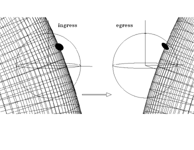
Figure 4: (Top) The accretion spot profile on ingress (from cycle 29995) and egress (the average of cycles 29982, 29993 and 29995). The profiles are constructed by subtracting successive intensities over 1 s time intervals. The ordinate of the upper plot is inverted to facilitate comparison. (Bottom) The view of the eclipsing limb at accretion region mid-ingress and mid-egress. The accretion region subtending $15^{\circ}$ is drawn to scale. The radius of the white dwarf is assumed to be 0.017$a$, where $a$ is the binary separation.

In those cycles where we have absolute time information (29994 and 29995) the egress takes place at $\phi=1.0413$ in both cycles, 10 s later than predicted by the linear ephemeris. This indicates that the observed-minus-calculated (O-C) residuals in Schwope et al. (2001) Figure 4 are continuing to increase. In case there are systematic differences between the optical and soft X-ray egress times, we rephased the Harrop-Allin (1999) data in their Figure 1 on the new ephemeris, including the UTC-TDB time correction of 59 s appropriate to the Schwope et al. (1997) ephemeris epoch. The data were taken on cycles $\sim 1322$ in Figure 4 of Schwope et al. (2001), and the O-C of $-1.6$ s is in agreement to within $\sim 1$ s with those determined from the soft X-ray data. The continuing increase in O-C residuals is an indication that the period in the linear ephemeris of Schwope et al. (2001) is slightly too short, and is in the opposite sense to that expected from their quadratic ephemeris which predicts a decrease in the O-C residuals. A period of 0.0868204212 days would eliminate the 10 s residuals we observe.

The duration of the eclipse from the centre of the accretion region ingress to the centre of its egress is $\Delta\phi=0.0778\pm 0.0002$ in cycles 29993, 29994 and 29995. This is the same as that found by Harrop-Allin et al. (1999b) of $\Delta\phi=0.0779\pm 0.0002$, and Schwope et al. (1997) of $\Delta\phi=0.0779$. The lack of variation in the duration of the eclipse is remarkable and implies that the accretion spot is at the same latitude for these observations. On the other hand, this is shorter by 6 s than the $0.0782-0.0792$ modelled by Schwope et al. (2001) from the soft X-ray eclipses, where the ingress was uncertain due to the low countrate and absorption.

For a particular mass ratio, the width of the eclipse determines the inclination of the system. Using $q=M_{2}/M_{1}=0.25$ (Schwope et al. 2001), the inclination is $85.0^{\circ}$ (assuming $M_{1}=0.9M_{\odot}$ and $\beta=40^{\circ}$, $\zeta=50^{\circ}$, where $M_{1}$ is the mass of the white dwarf and $\beta,\zeta$ are the magnetic longitude and colatitude of the accretion region. These correct for the location of the accretion spot on the surface of the primary; see below).

4.3 Stream eclipse variations

Complete ingress of the stream occurs at $\phi=0.982,0.979,0.977$ and $0.982$ for eclipses 29982, 29993, 29994 and 29995 respectively. During the period of complete eclipse the secondary is the only contributor to the light curve and provides a constant contribution which is greatest in the red band, as expected, with no contribution in the blue band.

Figure 5 shows more clearly that the observations reach total stream eclipse at different phases even though the spot ingresses/egresses both occur at the same time. This rapid change in the accretion flow$\--$magnetic field interaction between successive eclipses was first observed by Glenn et al. (1994) who found a difference in the time it took for the stream to be completely eclipsed of more than a minute between their two successive eclipses.

The shape of the accretion stream eclipse profile in the observed light curves gives a qualitative prediction of where brightness enhancements can be expected in the accretion stream. When the stream is brighter at later phases in the stream eclipse, as in cycles 29982 and 29995 (Figure 5), there must be more emission in the threading region, as this is the only part of the stream still visible. For the same reason, if the final stage of the stream eclipse takes place at later phases, the threading region must have moved: thus in cycles 29982 and 29995, either the accretion stream is brought further out from the line of centres during the ballistic part of the trajectory, or the magnetically channeled stream rises further out of the orbital plane (we address this in Section 5 below). This could be caused either by a small change in the location of the accretion spot on the primary surface, moving the accretion spot further from the line of centres, or perhaps a change in the velocity of the stream as it leaves the L₁ point. Likewise, if the accretion stream is fainter near the white dwarf, the system brightness will be fainter immediately after accretion region ingress. This may be the case for cycle 29995 (Figure 5).

Figure 5: The ingress and egress of eclipses 29982 (dotted), 29993 (dash-dot), 29994 (solid) and 29995 (dashed) smoothed over a running average of 20 s. The ordinates are normalised to 1 at the end of spot egress, and to 0 at total eclipse.

4.4 Colour variations

For cycle 29995 there is a rise in the yellow/red ratio during the stream ingress (Figure 2), so that successively more red light is blocked from the stream as the eclipse progresses. This implies that the last part of the stream to be eclipsed, near the threading region, emits relatively less at longer wavelengths than the rest of the stream. This rise is not evident in cycle 29993, but maybe present at a reduced level in cycle 29994 (Figure 3). This trend is consistent with a threading region which is increasingly hotter in the three successive eclipses. At the same time as the large yellow/red ratio change in cycle 29995 there is no change in the blue/yellow ratio.

After eclipse when the stream close to the primary is uncovered first, the different yellow/red ratios in cycles 29993 and 29995 are consistent with a hotter stream near the white dwarf in eclipse 29993 than in 29995. An increase in the blue/yellow ratio after eclipse is seen in all three cycles (29993, 29994 and 29995) and also implies that the magnetically confined stream material is becoming hotter towards the threading region.

The pre-eclipse dip around $\phi\approx 0.87$ in cycle 29994 (Figure 3) is also slightly bluer than at earlier or later phases. This was also the case in the light curves of Harrop-Allin et al. (1999b).

5 Indirect imaging

5.1 Methodology

We have inferred from a qualitative analysis of the light curves that the trajectory and/or intensity of the stream varies over successive orbital periods, and we can identify brightness enhancements along the stream length. However, it is more difficult to infer the location of the brightness enhancements without a model for the stream trajectory. In particular, at stream ingress there is no information on which parts of the stream are eclipsed at which phases. We can use an eclipse mapping method to create a model accretion stream by placing model stream points along a predetermined trajectory, consisting of a ballistic part from the L₁ point, coupling to a magnetically confined section where the material is threaded by the field lines of the white dwarf. The distance from the white dwarf where this transition occurs is the threading radius $R_{\mu}$, and is a user input to the model. The model system is rotated while the Roche lobe filling secondary eclipses the stream and white dwarf, with the brightness of the visible model stream points at each phase summed to form a model light curve. The resultant light curve is optimized with the genetic algorithm (GA) evolving the best fit light curve.

The ‘goodness of fit’ of a model light curve is measured with a ‘fitness function’ (see Harrop-Allin et al. 1999a for a full description). The GA adjusts the brightness points along the stream in an attempt to minimise this function, which consists of a $\chi^{2}$ term and a maximum entropy term, which ensures the problem is not under-constrained. After the final stages of the GA, a more conventional line-minimisation routine (Powell’s method) is used to reach the final minimum of the solution.

The accretion stream itself is taken to be physically thin in that it does not eclipse the primary, and so features such as the pre-eclipse dip (e.g. Watson 1995) are not reproduced by the model. However, the brightness contribution of each stream point is taken as the sine of the angle between the line of sight and the tangent to the stream at that point, essentially a projection effect, thus optically thick. We also exclude the white dwarf from the model, although the egress of the white dwarf can be seen in the light curves immediately before the egress of the accretion region.

The exact method we apply for the modelling is different to that of Harrop-Allin et al. (1999b, 2001) in that we are not applying the technique to the complete eclipse light curves, nor can we interpret the results in the same manner. There are a number of reasons for this. Firstly, and importantly, our observations are all truncated, either in the ingress or the egress of the accretion stream. For observations where the egress is truncated (cycle 29995), the model has difficulty breaking the ambiguity which exists when assigning brightness to points eclipsed in the same phase interval, i.e. the brightness can be either in the magnetically confined region or the ballistic. For observations where the pre-eclipse light curve is missing, we lack information on the accretion region, and parts of the stream towards the secondary (cycle 29993). A further difficulty lies in determining the nature of the variable emission from the accretion region. This is particularly important at egress, where the brightness of the spot can greatly affect the brightness distribution towards the white dwarf. After the egress of the accretion region the light curve consists of a variable component, plus the stream, which changes rapidly over the course of the observation. We have therefore chosen to use a restricted modelling technique, which relies on the ingress of the accretion stream alone. This means that we have truncated the light curves, removing all phases up to and including the ingress of the accretion region, and those after $\phi=1.0$. This is the only part of the light curve unaffected by the variable emission from the accretion region. We still have the problem of the ambiguity of the stream points, but we can make some progress in interpreting our results by referring back to the light curves and the colour ratios.

5.2 Fixed parameters and $R_{\mu}$

A number of parameters is required to produce a model light curve and reproduce the stream brightness distribution. These fall into two types: physical parameters such as the masses of the two component stars, and geometric parameters such as the location of the accretion region on the white dwarf (see Harrop-Allin et al. 1999a for details). The model is particularly sensitive to the exact value chosen for the parameter $R_{\mu}$, but we can constrain the value using the model stream geometry. If the value is too large then the model needs to assign a large amount of brightness to a few points. Conversely if $R_{\mu}$ is too small then no emission is assigned by the model to the points in the threading region. From brightness maps for a range of values of $R_{\mu}$ we can determine the end point of the ballistic trajectory and so provide a constraint on the value of $R_{\mu}$. We have found from our model fits of the light curves used here that the technique depends heavily on the data being of a sufficiently high signal-to-noise ratio, which is important because of the sensitivity to the value of $R_{\mu}$. Therefore, in order to determine the best fit value to use we further restrict the application of our model technique to cycles 29993 and 29995 (Figure 2).

Figure 6 shows model fits to the ‘blue’ light curve of cycle 29995 for different values of $R_{\mu}$. The stream maps highlight the dependence of the fits on a correct value for $R_{\mu}$. For a value of $R_{\mu}=0.18a$ the brightness of the threading region is low. This lack of emission, or ‘hole’, is caused by $R_{\mu}$ being too small - the data are incompatible with emission at the end part of the resulting long ballistic stream. On the other hand, if $R_{\mu}$ is too large, so that the model ballistic stream is shorter than it is in reality, a pile up of excess brightness at the threading region is seen, as in the stream map for $R_{\mu}=0.26$. The inappropriateness of the latter can be deduced from the poor fit to the region at $\phi=0.98$ (corresponding to the threading region) for values of $R_{\mu}$ which are too large (insets to Figure 6).

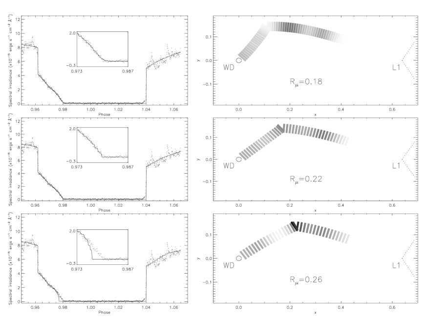
Figure 6: Fits to the ‘blue’ light curve of cycle 29995 with different values for the threading radius $R_{\mu}$ (0.18$a$, 0.22$a$ and 0.26$a$). The stream brightness maps on the right are gray scale plots with brighter stream emission being represented as darker. The gradual closing of a ‘hole’ at $R_{\mu}$ illustrates the sensitivity of the model to its location. The insets in the left hand panels show a close-up view of the fit at the threading region. For this cycle the value of $R_{\mu}=0.22a$ represents the best stream trajectory.

For all our modelling we used fixed values of $M_{1}=0.9M_{\odot}$, $q=0.25$ and $i=85.0^{\circ}$ (Harrop-Allin et al. 1999b, Schwope et al. 2001). Table 2 gives the values of $R_{\mu}$ and the field orientation parameters for each cycle. We estimate the range on the values of $\beta$ and $\zeta$ as $\pm 10^{\circ}(1\sigma)$.

The values of the three parameters in Table 2 are different from those found by Harrop-Allin et al. (1999b). We find $R_{\mu}=0.22\--0.26a$ ($1.3\times 10^{10}$ cm to $1.6\times 10^{10}$ cm), whereas Harrop-Allin et al. (1999b) found $R_{\mu}=0.17\--0.20a$. We can attribute this difference to an improved stream trajectory compared to that of Harrop-Allin et al. (1999a). This arises from an incomplete treatment of the appropriate forces in the frame of reference chosen by Harrop-Allin et al. (1999a). The difference is small, but for the angles used here the resulting $R_{\mu}$ is significantly different, with the Harrop-Allin et al. trajectory underestimating the values for $R_{\mu}$.

The decrease in the value of $R_{\mu}$ from cycle 29993 to 29995 implies that the stream penetrates further into the magnetosphere before threading onto the magnetic field lines (Figure 8). The effect of the change in the threading radius can be seen in Figure 5. The values of $\beta\sim 60^{\circ}$, $\zeta\sim 40^{\circ}$ found here are also larger than those used by Harrop-Allin et al. (1999b), but consistent within the uncertainties. Any change in these parameters would imply that the location of the accretion spot has moved further from the line of centres and the altered geometry of the magnetic field carries the accretion stream further round the white dwarf from the line of centres (see Section 5). They are in agreement with those found by Schwope et al. (2001) (their figure 6).

Table 2: The values of the coupling radius ($R_{\mu}$) and location of the accretion spot ($\beta$ and $\zeta$, magnetic longitude and colatitude respectively) for cycles 29993 and 29995. Values of $\beta$ and $\zeta$ have an estimated range of $\pm 10^{\circ}(1\sigma)$.

Cycle number	$R_{\mu}$	$\beta$	$\zeta$
29993	0.26$a$	55∘	30∘
29995	0.22$a$	60∘	40∘

5.3 Model results

With the values of $R_{\mu}$ determined above, we can use the model to find the best fit brightness map, from which we can then determine the brightness per unit stream length along the stream trajectory. This will show the brightness independent of the actual length of the stream eclipsed in any particular phase interval. This is important as there are different lengths of ballistic and magnetically confined stream eclipsed in a given phase interval.

Figure 7 presents the results of the modelling in two columns representing the two cycles presented here and the three rows the three energy bands: red, yellow and blue. We have divided the stream into three sections, as illustrated in Figure 8, which enclose the section nearest the white dwarf, the threading region and the stream in between the two. The ordinate then represents the total brightness of points eclipsed in these intervals per unit stream length, that is points in the ballistic and magnetically confined sections of the stream eclipsed in that phase range. The results have been calibrated into energy units using the standard star observation in order to facilitate comparison between the different bands. However the calibration is only approximate due to a lack of a standard star on the second night of observations.

Figure 7: The above plot shows for cycles 29993 and 29995, in each band, the total brightness per unit stream length in three sections of the stream. These intervals include a section of the ballistic trajectory plus those parts of the stream nearest the white dwarf (section 1), the threading region (section 3) and the magnetically confined stream between the two (section 2), c.f. Figure 8. A brightness enhancement at the threading region is evident in both cycles, but an enhancement towards the white dwarf is not seen in the red and yellow bands of cycle 29995.

Figure 8: The upper plot shows the model stream points for cycles 29993 and 29995 looking parallel to the orbital plane, while the lower plot shows them looking down onto the orbital plane. The difference in the stream trajectories is evident. The shaded regions are three equal phase intervals encompassed by the ingress of the white dwarf and the final ingress of the threading region for cycle 29993. These correspond to those parts of the stream used to form sections 1, 2 and 3 in Figure 7. (For cycle 29995 the definitions are equivalent.)

We can see from Figure 7 that there is enhanced brightness in the section containing the threading region in all bands in cycle 29993, but only in the yellow and blue in cycle 29995. The section containing those parts of the stream nearest the white dwarf are also bright in cycle 29993. However, in cycle 29995 this is only seen in the blue. The brightness of the different sections is consistent with the colour ratios from Section 4.4. In Figure 7 the threading region in cycle 29995 is hotter than that in cycle 29993 as the ratio of the yellow to red is greater for cycle 29995. This is again consistent with the colour ratios (Section 4.4). However, the blue to yellow ratio is similar in the two eclipse ingresses suggesting that the increase has occurred in both blue and yellow bands.

6 Discussion

6.1 Comparison with earlier results

The model fits of Harrop-Allin et al. (1999b) and Harrop-Allin (1999) for one pole accretion, show a general enhancement in the threading region and towards the white dwarf. Some eclipses (for example cycle 3723 and 3724 in Harrop-Allin 1999) show significantly greater brightness in the threading region of the white dwarf than others (such as the immediately preceding cycle 3722).

Enhanced brightness regions are also found by Vrielmann & Schwope (2001) and Kube et al. (2000) who apply similar modelling techniques. Vrielmann & Schwope (2001) apply their Accretion Stream Mapping technique to H$\beta$, H$\gamma$ and He ii $\lambda$ 4686Å observations of HU Aqr. They find a brightness enhancement at the threading region, but not towards the white dwarf, similar to cycle 29995, so implying that this may be absent in their emission lines. Kube et al. (2000) used the Civ $\lambda$ 1550Å line emission from UZ For, with a 3-dimensional stream model. They found three regions of enhanced brightness: one on the ballistic accretion flow, and two on the magnetically confined section. They suggest that the enhancements on the magnetically confined section are caused by irradiation of denser sections of the stream with a large area near the accretion region, and a smaller region near to the threading region. This may be the case in cycle 29993, where we find a bright stream near the white dwarf, and again near the threading region. Although Kube et al. find no enhancement actually at the threading region, this may be a result of an increase in the density of the stream as it approaches this point, resulting in an increase in the continuum optical depth, and hence a decrease of the Civ $\lambda$ 1550 Å equivalent width, and so is not necessarily indicative of a faint stream at this region.

6.2 Heating in the magnetically confined stream

Heating of the magnetic section of the stream has been modelled by Ferrario & Wehrse (1999) for a stream which is assumed to thread onto the field lines at a coupling radius $r_{c}$ (our $R_{\mu}$) from the white dwarf, over a radial distance $\Delta r_{c}$ in the orbital plane. This provides an opportunity for a comparison between our observationally derived results, and the main points of their theoretical model results.

Ferrario & Wehrse (1999) consider two heating mechanisms: irradiation by the X-ray component from the accretion shock (the soft X-rays being up to $\approx 4000$ times more efficient at heating the stream than the hard X-rays) and the effects of magnetic reconnection in the stream-field interaction over the threading region $\Delta r_{c}$. The comparison we make with these theoretical models is qualitative as the geometrical structure of the magnetically confined accretion flow in Ferrario & Wehrse is funnel-shaped, compared to our linear trajectory. However, our results showing brightness enhancements towards the threading region are consistent with their models which incorporated magnetic heating in the threading region. This implies that some magnetic heating mechanism is needed.

6.3 Temporal variations in the stream profile

Based on the colour ratios we deduced that the threading region was brighter and hotter in cycle 29995 than in cycle 29994 (Section 4.4). There are therefore significant changes in the threading region on the timescale of the orbital period (125 mins).

Although we have only modelled two cycles here, we can see that there is a difference in the brightness confirming the variability seen in the colour ratios and in the stream eclipse profiles from the light curves (see Figure 5). The large brightness enhancement near the white dwarf in cycle 29993 could be irradiated material which cools over the timescale of the next orbital period, leaving a fainter region as seen in cycle 29995 where the observed enhancement is less pronounced. However, without the model of the intermediate cycle, which we have excluded for reasons discussed previously, we cannot be certain and it will require more high signal-to-noise ratio observations of consecutive eclipses to investigate whether this in fact occurs. What is clear from the model results, and indeed directly from the raw light curves and colours, is that the emission from the whole stream is highly dynamic and unstable.

Dramatic changes in the stream eclipse profiles were also observed in the low state (Harrop-Allin et al. 2001, Glenn et al. 1994). These cycle-to-cycle changes in stream brightness and trajectory require a revision in our view of the stream, and in the manner in which the magnetic heating takes place in the threading region. Future treatments may need to consider large scale magnetic instabilities, and quasi-cyclic behavior.

7 Summary and conclusions

We have carried out high signal-to-noise ratio observations of HU Aqr using S-Cam2 on the WHT on two nights. The system was in a high accretion state, and from the single sharp change in the eclipse profile and archive soft X-ray light curves in this state, we infer that matter was accreting at only one pole on the white dwarf. At the onset of the eclipse, the accretion stream is the source of more than half of the optical emission from the system. The system brightness was similar from orbit to orbit, and the eclipse duration remained constant, but the shape of the accretion stream eclipse changed significantly, ending at $\phi=0.979$, $0.977$ and $0.982$.

We find eclipse durations which are unchanged from past optical studies (Harrop-Allin et al.  1999b, Schwope et al. 1997), but shorter than those deduced in the soft X-rays by Schwope et al. (2001). However, the location of the accretion region is similar to that found by Schwope et al. (2001), so that there is no evidence that the optical emission is from higher latitudes on the white dwarf than the soft X-rays. This indicates that the duration of the soft X-ray eclipses may be affected by absorption, as they suggested.

The duration of the egress of the accretion region in the optical is $8$ s, compared to $1.3$ s in soft X-rays (Schwope et al. 2001). This indicates clearly that the region emitting cyclotron radiation is extended by a factor of $\sim 5$ by comparison with the soft X-ray emitting region, which Schwope et al. (2001) calculated as subtending an angle of $3^{\circ}$.

We have found significant changes in the colour of the accretion stream from one eclipse to the next. This indicates that the threading region is hottest in the last of the eclipses by comparison with the previous two (see Section 4.4). We have modelled the stream using the technique of Hakala (1995) and Harrop-Allin et al. (1999a). This finds that most of the emission originates from two places, the region close to the white dwarf and in the threading region. By comparison with the models of Ferrario & Wehrse (1999) this indicates that magnetic heating is required in the threading region. The modelling clearly identifies an increase in brightness in the threading region for both cycles and an enhancement towards the white dwarf for cycle 29993. From this change in brightness of the heated regions in the model streams, and the varying stream eclipse profiles, we suggest that the magnetic heating in the threading region may be unstable. The implications of the highly variable stream trajectory and brightness profile should be recognised in future investigations of the stream properties. A systematic study of series of consecutive eclipses, with the highest possible signal-to-noise ratio, is required to investigate the characteristics of the magnetic heating and stream instabilities.

References

- [1] Blackburn J., 1995, in Shaw R. A., Payne H. E., Hayes J. J. E., eds, Astronomical Data Analysis Software and Systems IV. ASP Conf. Ser. 77, San Francisco, p. 367
- [2] de Bruijne J.H.J., Reynolds A.P., Perryman M.A.C., Favata F., Peacock A., 2001, Analysis of astronomical data from optical superconducting tunnel junctions, in Focal plane detector array developments, eds. Z. Ninkov, W.J. Forrest, Opt. Eng. (The International Society for Optical Engineering; SPIE), in press (astro-ph/0108232)
- [3] de Bruijne J.H.J., Reynolds A.P., Perryman M.A.C., et al., A&A, 2002, 381, 57
- [4] Case D. V., 1996, M.Phil. thesis, University of Keele
- [5] Cropper M., 1990, Space Sci. Rev., 54, 195
- [6] Glenn J., Howell S. B., Schmidt G. D., Liebert J., Grauer A. D., Wagner R. M., 1994, ApJ, 424, 967
- [7] Ferrario L. & Wehrse R., 1999, MNRAS, 310, 189
- [8] Hakala P. J., 1995, A&A, 296, 164
- [9] Harrop-Allin M. K., 1999, PhD Thesis, University of London
- [10] Harrop-Allin M. K., Hakala P. J., Cropper M., 1999a, MNRAS, 302, 362
- [11] Harrop-Allin M. K., Cropper M., Hakala P. J., Hellier C., Ramseyer T., 1999b, MNRAS, 308, 807
- [12] Harrop-Allin M. K., Potter S. B., Cropper M., 2001, MNRAS, 326, 788
- [13] Howell S. B., Nelson L. A., Rappaport S., 2001, ApJ, 550, 897
- [14] Kube J., Gänsicke B. T., Beuermann K., 2000, A&A, 356, 490
- [15] Perryman M. A. C., Foden C. L., Peacock A., 1993, Nuc. Inst. Meth. A, 325, 319
- [16] Perryman M. A. C., Favata F., Peacock A., Rando N., Taylor B. G., 1999, A&A, 346, 30
- [17] Perryman M. A. C., Cropper M., Ramsay G., Favata F., Peacock A., Rando N., Reynolds A., 2001, MNRAS, 324, 899
- [18] Rando N., Verveer J., Andersson S., et al., 2000, Rev. Sci. Inst., 71(4582)
- [19] Schwope A. D., Mantel K-H., Horne K., 1997, A&A, 319, 894
- [20] Schwope A. D., Schwarz R., Sirk M., Howell S. B., 2001, A&A, 375, 419
- [21] Sohl K. & Wynn G., 1999, in Hellier C., Mukai K., eds, ASP Conf. Ser. Vol. 157, Annapolis Workshop on Magnetic Cataclysmic Variables. Astron. Soc. Pac., San Francisco, p. 87
- [22] Vrielmann S. & Schwope A. D., 2001, MNRAS, 322, 269
- [23] Warner B., 1995, Cataclysmic variable stars. Cambridge Univ. Press, Cambridge Watson M. G., 1995, in Buckley D. A. H., Warner B., eds, ASP Conf. Ser. Vol. 85, Cape Workshop on Magnetic Cataclysmic Variables. Astron. Soc. Pac., San Francisco, p. 179