Hydrogen wall and heliosheath Ly-$\alpha$ absorption toward nearby stars: possible constraints on the heliospheric interface plasma flow

Abstract

In this paper, we study heliospheric Ly-$\alpha$ absorption toward nearby stars in different lines of sight. We use the Baranov-Malama model of the solar wind interaction with a two-component (charged component and H atoms) interstellar medium. Interstellar atoms are described kinetically in the model. The code allows us to separate the heliospheric absorption into two components, produced by H atoms originating in the hydrogen wall and heliosheath regions, respectively. We study the sensitivity of the heliospheric absorption to the assumed interstellar proton and H atom number densities. These theoretical results are compared with interstellar absorption toward six nearby stars observed by the Hubble Space Telescope.

Izmodenov et al. Hydrogen wall and heliospheric absorption Sometime 2002 ????? 2002???00021 AGU2002 Vlad Izmodenov, Lomonosov Moscow State University, Department of Aeromechanics and Gas Dynamics, Faculty of Mechanics and Mathematics, Moscow, 119899, Russia (izmod@ipmnet.ru) Brian Wood, JILA, University of Colorado, and NIST, Boulder, CO 80309-0440 (woodb@casa.colorado.edu) Rosine Lallement, Service d’Aeronomie, CNRS, F-91371, Verrieres le Buisson, France (Rosine.Lallement@aerov.jussieu.fr)

1 Introduction

The solar system is traveling in the surrounding Local Interstellar Cloud (LIC). In the 1960s, it was realized [e.g., Patterson et al., 1963; Fahr, 1968; Blum and Fahr, 1970] that interstellar atoms penetrate deep into the heliosphere and, therefore, can be observed. The interstellar atoms of hydrogen have been detected by measurements of the solar backscattered Ly-$\alpha$ irradiance [Bertaux and Blamont, 1971; Thomas and Krassa, 1971]. Later, interstellar atoms of helium were also measured directly [Witte et al., 1996] and indirectly as backscattered solar irradiance [Weller and Meier, 1981; Dalaudier et al., 1984]. At present, there is no doubt that inside the heliosphere, properties of He atoms such as temperature and velocity are different from those of H atoms. In particular, the H atoms are decelerated and heated compared with atoms of interstellar helium inside the heliosphere [Lallement et al., 1993; Costa et al., 1999; Lallement, 1999]. The reason for this is a stronger coupling of H atoms with plasma protons in the heliospheric plasma interface through charge exchange. Many works developed the concept of the heliospheric plasma interface over more than four decades after pioneering papers by Parker [1961] and Baranov et al. [1970].

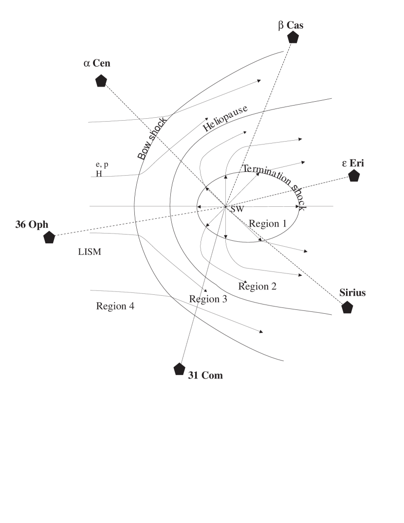
Figure 1: The heliospheric interface is the region of the solar wind interaction with LIC. The heliopause is a contact discontinuity, which separates the plasma wind from interstellar plasmas. The termination shock decelerates the supersonic solar wind. The bow shock may also exist in the interstellar medium. The heliospheric interface can be divided into four regions with significantly different plasma properties: 1) supersonic solar wind; 2) subsonic solar wind in the region between the heliopause and termination shock (i.e., the heliosheath) ; 3) disturbed interstellar plasma region (or ”pile-up” region) around the heliopause; 4) undisturbed interstellar medium.

The heliospheric interface is formed by the interaction of the solar wind with the charged component of the interstellar medium (see Figure 1). The heliospheric interface is a complex structure having a multi-component nature. The solar wind and interstellar plasmas, interplanetary and interstellar magnetic fields, interstellar atoms, Galactic and anomalous cosmic rays (GCRs and ACRs), and pickup ions all play prominent roles. Interstellar hydrogen atoms interact with the heliospheric interface plasma by charge exchange. This interaction significantly influences both the structure of the heliospheric plasma interface and the flow of the interstellar H atoms. In the heliospheric interface, atoms newly created by charge exchange have the properties of local protons. Since the plasma properties are different in the four regions of the heliospheric interface shown in Figure 1, the H atoms in the heliosphere can be separated into four populations, each having significantly different properties. For example, population 3 consists of the atoms created by charge exchange with relatively hot protons in the region of disturbed interstellar plasma around the heliopause (region 3 in Figure 1). It was realized theoretically by Baranov et al. [1991] that the atoms of population 3 form a so-called “hydrogen wall” around the heliopause. The hydrogen wall is a significant enhancement of the density of interstellar atoms of hydrogen around the heliopause compared with the number density of the undisturbed local interstellar medium. The self-consistent models of the heliospheric interface predict that the secondary interstellar atoms (or atoms of population 3) are decelerated and heated compared with the original interstellar H atoms.

The Ly-$\alpha$ transition of atomic H is the strongest absorption line in stellar spectra. Thus, the heated and decelerated atomic hydrogen within the heliosphere produces a substantial amount of Ly-$\alpha$ absorption. This absorption, which must be present in all stellar spectra since all lines of sight go through the heliosphere, has been unrecognized until recently, because it is undetectable in the case of distant objects characterized by extremely broad interstellar Ly-$\alpha$ absorption lines that hide the heliospheric absorption. We know now that in the case of nearby objects with small interstellar column densities, it can be detected in a number of directions. The heliospheric absorption will be very broad, thanks to the high temperature of the heliospheric H, and its centroid will also generally be shifted away from that of the interstellar absorption due to the deceleration, allowing its presence to be detected despite the fact that it remains blended with the interstellar absorption. The hydrogen wall absorption was first detected by Linsky and Wood [1996] in Ly-$\alpha$ absorption spectra of the very nearby star $\alpha$ Cen taken by the Goddard High Resolution Spectrograph (GHRS) instrument on board the Hubble Space Telescope (HST). Since that time, it has been realized that the absorption can serve as a remote diagnostic of the heliospheric interface, and for stars in general, their “astrospheric” interfaces.

The $\alpha$ Cen line of sight lies 52^∘ from the upwind direction of the interstellar flow through the heliosphere. An additional detection of heliospheric H I absorption only 12^∘ from the upwind direction was provided by HST observations of 36 Oph [Wood et al., 2000a]. For downwind lines of sight, the heliospheric absorption is also not negligible [Williams et al., 1997]. Analysis of Ly-$\alpha$ absorption toward Sirius shows that absorption of atoms of population 2 created in the heliosheath (see Figure 1) is needed in addition to interstellar and “hydrogen wall” absorption components in order to explain observations [Izmodenov et al., 1999].

In addition to heliospheric absorption, “astrospheric” absorption towards Sun-like stars was detected by Wood et al. [1996], Dring et al. [1997], and Wood and Linsky [1998]. These observations might be used to infer properties of these stars and their interstellar environments [Wood et al. 2001; Müller et al., 2001].

A theoretical model of the heliospheric interface should be employed to interpret observations and put constraints on the local interstellar parameters and the heliospheric interface structure. This model should self-consistently take into account plasma and H atom components. Since the mean free path of H atoms is comparable with the size of the heliospheric interface, the H atom flow needs to be treated kinetically through the velocity distribution function, which is not Maxwellian [Baranov et al., 1998; Müller et al., 2000; Izmodenov et al., 2001]. Recently, Wood et al. [2000b] compared observations of Ly-$\alpha$ toward six nearby stars with model-predicted absorption. Both a Boltzmann mesh code [Lipatov et al., 1998] and a multi-fluid approach [Zank et al., 1996] were used to compute H atom distributions in the heliosphere. In comparing these models with the data, it was found that the kinetic models predict too much absorption. Models created assuming different values of the interstellar temperature and proton density fail to improve the agreement. Surprisingly, it was found that a model that uses a multifluid treatment of the neutrals rather than the Boltzmann particle code is more consistent with the data [Wood et al., 2000b].

In this paper, we continue to study heliospheric absorption toward these stars. In our study, we use the Baranov-Malama model [Baranov and Malama, 1993, 1995, 1996] of the heliospheric interface, which is described in the next section. This model uses a Monte Carlo code with splitting of trajectories, which allows very precise computation of H atom distributions. Another advantage of the model is the possibility of separating of heliospheric H atoms into several populations, as discussed above. This model advantage allows us to consider separately two types of heliospheric absorption, hydrogen wall absorption and heliosheath absorption.

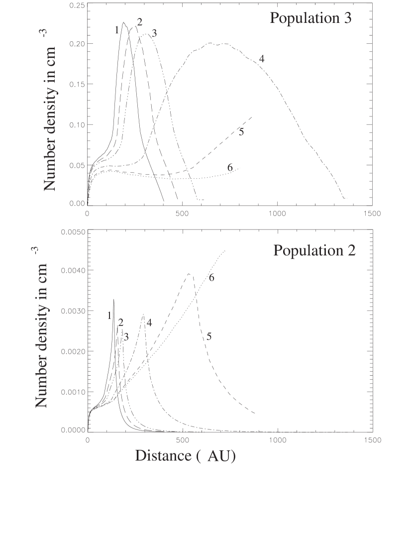
Figure 2: Density distributions of H atoms of population 3, atoms originated in the disturbed interstellar medium (region 3 in figure 1), and population 2, atoms originated in the heliosheath (region 2 in figure 2). Density distributions are shown as functions of heliospheric orientation relative to different line of sights. Curves 1, 2, 3, 4, 5, and 6 correspond to $\theta=12^{\circ}$, $52^{\circ}$, $73^{\circ}$, $112^{\circ}$, $139^{\circ}$, and $148^{\circ}$, respectively, where $\theta$ is the angle relative to the upwind direction of the interstellar flow. The figure shows the number densities for model 3 (see Table 1).

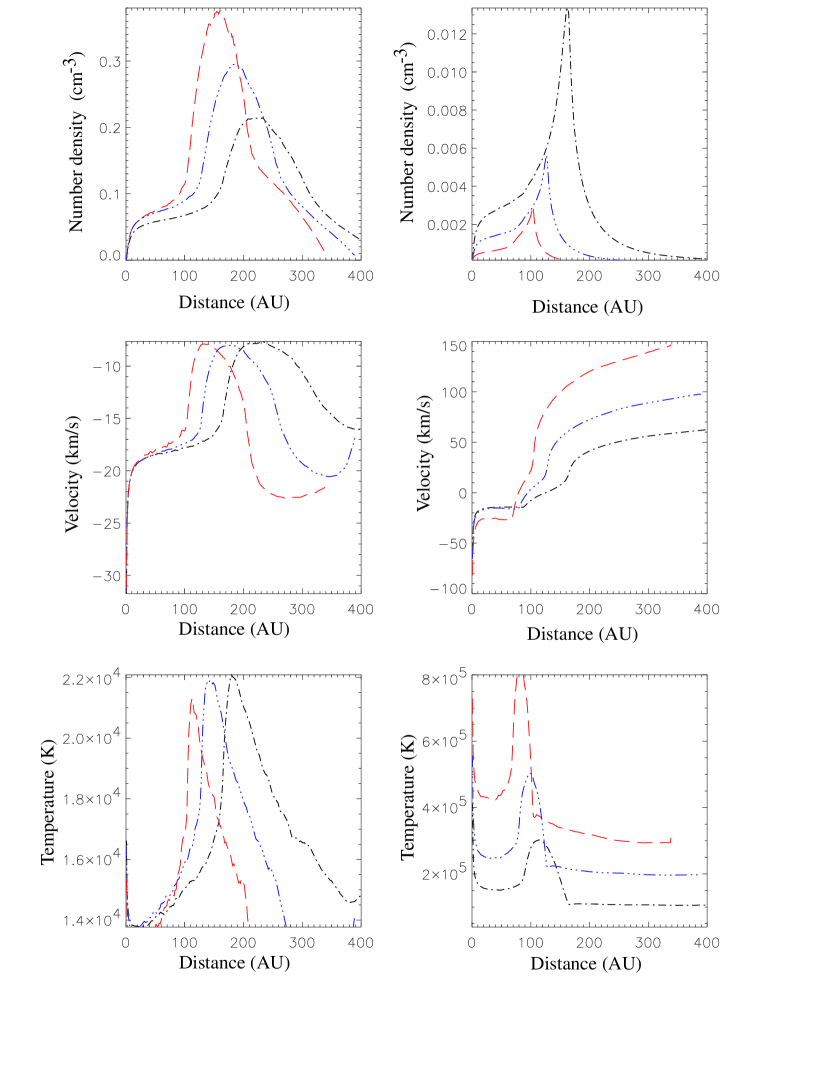
Figure 3: Number densities (upper row), velocities (middle row), and effective temperatures (lower row) of population 3 (left column) and population 2 (right column) toward 36 Oph. Dot-dash lines correspond to model 4, dot-dot-dot-dash lines correspond to model 5 and long dashes correspond to model 6 (see Table 1).

2 Heliospheric interface model

To calculate heliospheric absorption we employ the Baranov-Malama model of the solar wind interaction with the two-component interstellar medium [Baranov and Malama, 1993, 1995, 1996; Izmodenov, 2000]. This is an axisymmetric model, where the interstellar wind is assumed to have uniform parallel flow, and the solar wind is assumed to be spherically symmetric at the Earth’s orbit. Plasma and neutral components interact mainly by charge exchange. However, photoionization, solar gravity, and solar radiation pressure, which are especially important in the vicinity of the Sun, are also taken into account in the model. The process of electron impact ionization, which is important in the heliosheath [Baranov and Malama, 1996], is taken into account as well. Kinetic and hydrodynamic approaches were used for the neutral and plasma components, respectively. The kinetic equation for the neutrals is solved together with the Euler equations for a one-fluid plasma. The influence of the interstellar neutrals is taken into account in the right-hand side of the Euler equations that contains source terms [Baranov and Malama, 1993; Malama, 1991], which are integrals of the H atom distribution function $f_{H}(\vec{V}_{H})$ and can be calculated directly by a Monte Carlo method [Malama, 1991]. The set of kinetic and Euler equations is solved by an iterative procedure suggested by Baranov et al. [1991]. Supersonic boundary conditions were used for the unperturbed interstellar plasma and for the solar wind plasma at Earth’s orbit. The velocity distribution of interstellar atoms is assumed to be Maxwellian in the unperturbed LIC.

Basic results of the model can be briefly summarized as follows [see also Izmodenov, 2000]. In the presence of interstellar H atoms the heliospheric interface is much closer to the Sun compared with the case of a fully ionized LIC. The termination shock becomes more spherical, and complicated shock structure in the tail disappears. The plasma flows are disturbed upstream of both the bow and termination shocks. This is an effect of H atoms that interact with protons by charge exchange. The solar wind is decelerated by $15-30$% as it approaches the termination shock. The Voyager spacecraft observe the deceleration of the solar wind at large heliocentric distances [Richardson, 2001]. The number density of pickup ions, which are created by charge exchange, may reach $20-50$% of the solar wind number density at the distance of the TS. The expected distance to the termination shock is $80-100$ AU and depends on local interstellar parameters. The interstellar atoms are significantly disturbed in the interface. Since the velocities of new atoms created by charge exchange depend on properties of the local plasma, it is convenient to distinguish four populations of atoms depending on the place of origin, as described above. The velocity distribution function of H atoms can be represented as a sum of the distribution functions of these populations. Izmodenov et al. [2001] studied the evolution of the four velocity distribution functions in the heliospheric interface.

Table 1: Sets of model parametersa

Model	$n_{H,LIC}$	$n_{p,LIC}$	Notation in figures
	$cm^{-3}$	$cm^{-3}$
1	0.10	0.10	solid
2	0.15	0.05	dotted
3	0.15	0.10	dashed
4	0.20	0.05	dot-dash
5	0.20	0.10	dot-dot-dot-dash
6	0.20	0.20	long dash

a$n_{H,LIC}$ and $n_{p,LIC}$ are local interstellar atom and proton number densities, respectively.

We computed the global heliospheric interface structure and distribution of interstellar hydrogen in the interface using the Baranov-Malama model. Our calculations assume the following values for the fully ionized solar wind at 1 AU: $n_{p,E}=6.5$ cm^-3, $V_{p,E}=450$ km s^-1, and $M_{E}=10$, where $n_{p,E}$, $V_{p,E}$ and $M_{E}$ are the proton number density, solar wind speed, and Mach number, respectively. For the inflowing partially ionized interstellar gas, we assume a velocity of 25.6 km s^-1 and a temperature of 7000 K. These values are consistent with in situ observations of interstellar helium [Witte et al., 1996]. Two other input parameters, interstellar proton and H atom number densities, are varied. The values assumed for these parameters for the various models are listed in Table 1. We vary $n_{p,LIC}$ in the range $0.1-0.2$ cm^-3, while $n_{H,LIC}$ is varied in the range $0.05-0.2$ cm^-3.

In principle, each of the four H atom populations produces an absorption line. However, populations 1 and 4 can be neglected here, for the following reasons. Population 4 atoms are unperturbed interstellar atoms (having not charge exchanged at any time), and the average temperature and velocity of this population in the heliosphere is very similar to those of the gas in the interstellar cloud beyond the heliosphere (there is a slight and negligible difference due to selection effects). Thus, the population 4 absorption cannot be distinguished from the interstellar absorption. Since the interstellar column-density is a fitted parameter, it will automatically include population 4. Moreover, this gas is not hot and the column density is small, resulting in an unnoticeable difference. Population 1 corresponds to atoms flowing away from the Sun at very large velocities (i.e., the speed of the neutralized supersonic solar wind protons). The produced absorption is thus strongly shifted and broadened due to solar wind inhomogeneities. Also, since column densities are very small, this absorption is very shallow and undetectable.

Figure 2 shows calculated number densities of populations 2 and 3, which are of interest in this paper, toward six selected line of sights from upwind to downwind. The figure shows the number densities for model 3 (see Table 1). The hydrogen wall (upper panel) is most pronounced in the upwind direction. However, the wall decreases slowly with increasing of the angle $\theta$ relative to the upwind direction ($\theta=0^{\circ}$ for upwind). At $\theta=112^{\circ}$ (curve 4) the wall is still only slightly lower than it is in the upwind direction. There is no hydrogen wall in downwind directions (curves 5 and 6). In upwind and crosswind directions, the number densities of population 2 are about two orders of magnitude less than number densities of population 3. However, the densities of populations 2 and 3 are different by only about one order of magnitude in the downwind directions (curves 5 and 6). Despite their small densities, the atoms of population 2 can produce noticeable absorption due to their higher temperature.

Figure 3 shows number densities, bulk velocities, and effective kinetic temperatures for models 4-6 toward 36 Oph. The highest hydrogen wall is for the model with the largest $n_{p,LIC}$ (model 6). Decrease of $n_{p,LIC}$ results in a decrease of the hydrogen wall. At the same time, the hydrogen wall becomes wider, so that the H column density does not vary significantly from model 4 to model 6. All models show approximately the same velocities and temperatures of population 3 in the hydrogen wall region, which produces most of the heliospheric absorption. In contrast to population 3, the number densities, velocities, and effective kinetic temperatures of population 2 vary significantly with $n_{p,LIC}$ (right column plots in Figure 3). These effects are connected with: a) the location of the termination shock, which is closer to the Sun for higher $n_{p,LIC}$, b) the width of the heliosheath region; and c) effects of interstellar H atoms filtration and their influence on the heliosheath plasma flow [for details, see Izmodenov, 2000; Izmodenov et al., 1999, 2001].

More results on the distribution of H atom and plasma parameters for the presented six models are provided at http://izmod.ipmnet.ru/ izmod/Papers/IWL/index.html. This page contains contour plots of plasma and H atom population number densities and velocities, and other supplemental information.

3 Modeling of heliospheric absorption

The absorption profile along a line of sight is

$$I(\lambda)=I_{0}(\lambda)exp(-\tau(\lambda)),$$ (1)

where $I_{0}(\lambda)$ is the assumed background Ly-$\alpha$ profile, and $\tau(\lambda)$ is the opacity profile. The opacity profile is

$$\tau=\frac{\pi e^{2}fN\lambda^{2}}{mc^{2}}\phi(\lambda).$$ (2)

Here, $f$ is the oscillator absorption strength, $N$ is the column density, and $\phi(\lambda)=(\lambda_{0}c\phi(v))/\lambda^{2}$, where $\phi(v)$ is the normalized velocity distribution along the line of sight. In the velocity space to which wavelengths can be linearly transferred, $v=c(1-\lambda_{0}/\lambda)$, where $\lambda_{0}$ is the rest wavelength of Ly-$\alpha$. In the case of a Maxwellian velocity distribution of the neutral gas, the absorption is determined by three parameters ($N$, $u$, $b$), and the absorption profile is

$$I(v)=I_{0}(v)exp(-\frac{\pi e^{2}fN\lambda_{0}}{mc}\frac{e^{-\frac{(v-u)^{2}}{b^{2}}}}{\sqrt{\pi}b}).$$ (3)

Here, $u$ and $b$ are line-of-sight bulk and thermal velocities, respectively. Since the column density of H atoms in the heliospheric interface is less than 10¹⁵ cm^-2, the extended Lorentzian wings of natural line broadening do not accumulate any appreciable opacity. Therefore, equation (3), which corresponds to pure Doppler broadening, is applicable. Note that for the interstellar absorption the column density is higher and one must take the Lorentzian wings into account and replace the Doppler profile in equation (3) with a Voigt profile:

$$I(v)=I_{0}(v)exp(-\frac{\pi e^{2}fN\lambda_{0}}{mc\sqrt{\pi}b}H(a,v-u)).$$ (4)

Here $a=\Gamma/4\pi b$, where $\Gamma=0.0755$ is the transition rate in km/s units, and

$$H(x,y)=\int^{\infty}_{-\infty}\frac{exp(-t^{2})dt}{(y-t)^{2}+x^{2}}.$$ (5)

Using the distributions of interstellar H atoms computed as discussed in the previous section, we compute the heliospheric absorption toward the six selected directions. To study common properties and variations of the heliospheric absorption from upwind to downwind, we assume in this section stellar profiles of $I_{0}(\lambda)=1$. We compute absorption produced by H atoms of population 3 and population 2 separately. Hereafter, these two absorption components will be called “hydrogen wall” and “heliosheath” absorption, respectively.

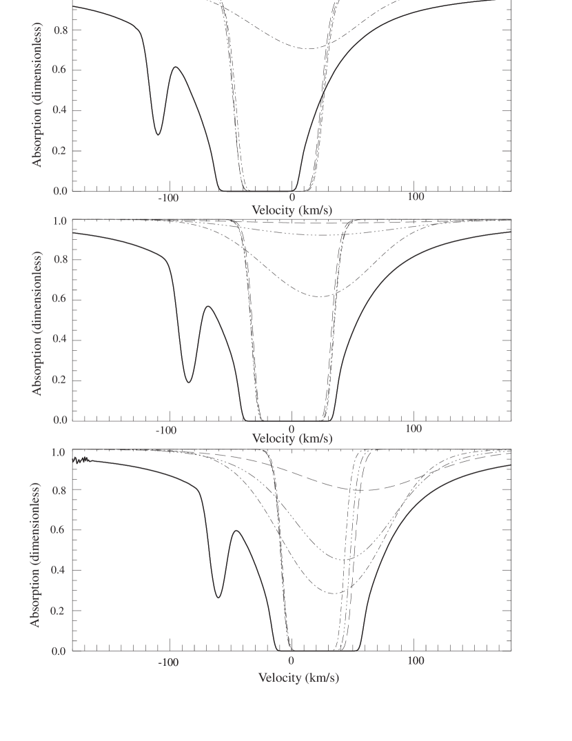
Figure 4: Simulated interstellar and heliospheric absorption of populations 2 and 3 toward 36 Oph (upper panel), 31 Com (middle panel), and Sirius (lower panel), which are located in the upwind (12^∘), crosswind (73^∘) and downwind (139^∘) directions, respectively. Interstellar absorption are shown by solid curves. Simulated hydrogen wall and heliosheath absorption are shown as dot-dash lines for model 4, dot-dot-dot-dash lines for model 5 and dash lines for model 6 (see Table 1). (The hydrogen wall absorption is the narrow, saturated absorption, while the heliosheath is the broader, unsaturated absorption.)

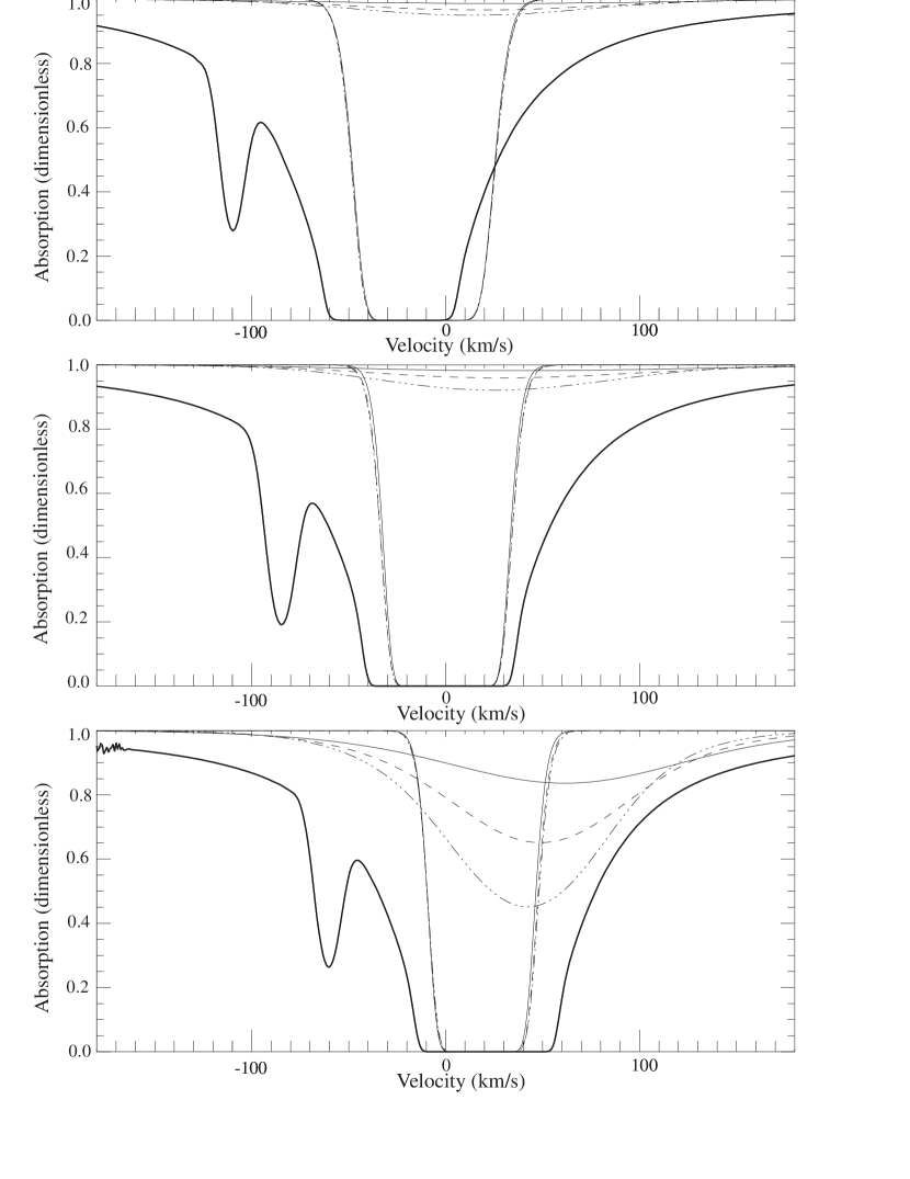
Figure 5: Same as figure 4, but for models 1 (solid lines), 3 (dashed lines), and 5 (dot-dot-dot-dashed lines).

Figures 4 and 5 present both calculated hydrogen wall and heliosheath absorption components for different models of the heliospheric interface toward three stars, representing nearly upwind (36 Oph), crosswind (31 Com), and downwind ($\epsilon$ Eri) directions. The absorption is shown in the heliospheric rest frame on a velocity scale. The expected interstellar absorption toward these stars is also shown in the figures in order to compare them with the heliospheric absorption. Details of the computation of the absorption are discussed in the next section. Figure 4 shows variations of heliospheric absorption with increase of the interstellar proton number density, $n_{p,LIC}$, from 0.05 cm^-3 (model 4) to 0.2 cm^-3 (model 6), with $n_{H,LIC}=0.2$ cm^-3 for all these models. Figure 5 shows variations of heliospheric absorption with an increase of $n_{H,LIC}$ from 0.10 cm^-3 (model 1) through 0.15 cm^-3 (model 3) to 0.2 cm^-3 (model 5), with $n_{p,LIC}=0.1$ cm^-3 for all these models.

Absorption of the hydrogen wall. All models produce nearly the same hydrogen wall absorption for upwind and crosswind directions. Downwind, the absorption is different for different models. But due to small column densities of population 3 in downwind directions, the absorption cannot be detected in stellar spectra. In the upwind direction, the atoms of population 3 are decelerated relative to the original interstellar atoms. Therefore, the absorption by population 3 is redshifted compared to the interstellar absorption. In nearly crosswind directions the projections of the bulk velocities to the direction of the Sun are close to zero for population 3 as well as for primary interstellar gas. Thus, the absorption of population 3 is hidden by saturated interstellar absorption and cannot be observed (middle panels in Figures 4 and 5).

Absorption in the heliosheath. In contrast to the hydrogen wall absorption, the heliosheath absorption varies significantly with the interstellar proton and H atom number densities. A higher number density of population 2 for models with smaller interstellar proton number density $n_{p,LIC}$ (see Figure 3) leads to large absorption for this model compared to models with larger $n_{p,LIC}$. Models with higher $n_{H,LIC}$ also predict more heliosheath absorption (see Figure 5) than models with small $n_{H,LIC}$. The difference between models increases for crosswind and downwind directions. Generally, for all models the heliosheath absorption is more pronounced in the crosswind and downwind directions. Toward these directions both the size of the heliosheath and the number density of population 2 are larger compared with upwind. The heliosheath absorption is redshifted in crosswind directions compared with the interstellar and hydrogen wall absorption components, and analysis of absorption toward crosswind stars might put particularly strong constraints on the heliosheath plasma structure.

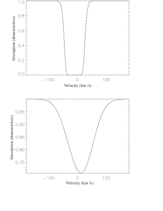
Figure 6: A comparision of absorption profiles calculated directly from distributions of H atoms (solid lines) with absorption profile approximations assuming uniform Maxwellian gases (dashed lines). The absorption profiles are shown toward the 36 Oph direction ($\theta=12^{\circ}$). Upper and bottom panels are for populations 2 and 3, respectively.

As seen from Figures 2 and 4, the parameters of heliospheric populations of H atoms have large variations in the heliospheric interface, as well as in each of its sub-regions. Moreover, the velocity distributions of the heliospheric populations are not Maxwellian [Izmodenov et al., 2000]. However, it is still interesting to see whether it is possible to model heliospheric absorption as if it were produced by uniform Maxwellian gases. Using the computed distribution functions, we take the zeroth, first, and second moments of the Maxwellian to compute $N$, $u$, and $b$. Then, we use these numbers to compute a Gaussian profile according to eq. (3). A comparison of the original profiles computed directly from the velocity distributions with the Gaussian profiles shows rather good agreement for both populations 2 and 3 (see Figure 6). Note that we compute Gaussian profiles and compare them with the exact profiles for populations 2 and 3 separately. If populations 2 and 3 were treated as one population, the Gaussian approximation would be much worse. Note that for some directions and models the difference between model predictions and their Gaussian approximations might be larger, and these fits should be used for interpretation with great caution.

It is important to note here that our model does not extend far enough downwind. Our computational grid extends only 700 AU in the downwind direction, which is not far enough to incorporate all heliospheric absorption [Izmodenov and Alexashov, in preparation]. Therefore, our calculations underestimate absorption in downwind directions ($\theta>125^{\circ}$).

Table 2: Information on stars and interstellar absorption.

Star	Angle	Distance	Interstellar parameters toward the stara
	from	(pc)	$u$	T	N	D/H,
	Upwind		(km s-1)	(K)	$\times$ 1017	$\times$ 10-5
					(cm-2)
36 Oph	$12^{\circ}$	5.5	-28.4	6200	7.80	1.25
$\alpha$ Cen	$52^{\circ}$	1.34	-18	5800	4.00	1.5
31 Com	$73^{\circ}$	90.9	-3.2	8000	8.3	1.75
$\beta$ Cas	$112^{\circ}$	13.9	9.1	9500	13.5	1.65
Sirius	$139^{\circ}$	2.7	19	6000	1.6	1.65
			13	6000	1.6	1.65
$\epsilon$ Eri	$148^{\circ}$	3.3	20.8	7300	7.6	1.45

a$u$,T,N are the interstellar velocity, temperature, column density and D/H ratio toward the star.

4 The observations, interstellar absorption, and stellar spectra

In this section, we use the heliospheric absorption models discussed above to analyze absorption spectra toward six nearby stars. For accurate study of the heliospheric absorption based on the analysis of observed absorption spectra, one needs to know both the original stellar Ly-$\alpha$ line profile and the interstellar absorption.

The Ly-$\alpha$ lines of these six stars observed by HST are shown in Figure 7 (left column). All of the spectra except that of 36 Oph A were taken using the Goddard High Resolution Spectrograph (GHRS) instrument. The 36 Oph A data were obtained by the Space Telescope Imaging Spectrograph (STIS), which replaced GHRS in 1997. The spectra are plotted on a heliocentric velocity scale. All show broad, saturated H I absorption near line center and narrower deuterium (D I) absorption about 80 km s^-1 blueward of the H I absorption. Figure 7 also shows the assumed intrinsic stellar Ly $\alpha$ lines and the best estimates for interstellar absorption. The interstellar parameters of these estimates are summarized in Table 2. The models suggest that heliospheric absorption will always be redshifted from the the ISM absorption regardless of the direction of the line of sight, while astrospheric absorption will conversely be blueshifted [Wood et al., 2000b; Izmodenov et al. 1999]. This is primarily because of the deceleration and deflection of neutral H at the bow shock, and because for the heliosphere we are observing the decelerated and deflected neutral H from inside the heliosphere while for astrospheres we are observing it from the opposite perspective outside the astrosphere. Thus, excess absorption on the red side of the Ly $\alpha$ absorption, when present, is interpreted as heliospheric absorption, while excess absorption on the blue side, when present, is interpreted as astrospheric absorption. In this paper we focus on the red side of the Ly $\alpha$ absorption since we are interested in the heliospheric absorption. The stellar profiles and interstellar absorption estimates are based on previously published work, which is summarized below.

$\alpha$ Cen. The $\alpha$ Cen data provided the first evidence for heliospheric absorption. Both members of the $\alpha$ Cen binary system were observed. Linsky and Wood [1996] demonstrated that the results of their analysis were the same for both the $\alpha$ Cen A and $\alpha$ Cen B data. It is the $\alpha$ Cen B spectrum that we display in Figure 7, since it has a somewhat higher signal-to-noise ratio (S/N) than the $\alpha$ Cen A data. Using the D I line to define the central velocity and temperature of the interstellar material, Linsky and Wood [1996] found they could not fit the $\alpha$ Cen H I profile with only interstellar absorption. In Figure 7, we show interstellar absorption toward $\alpha$ Cen with the D/H value equal to $1.5\times 10^{-5}$, which is the generally accepted LIC D/H value.

36 Oph. Wood et al. [2000a] analyzed the 36 Oph data. The analysis of the 36 Oph data proved to be very similar to that of $\alpha$ Cen, with the apparent existence of excess Ly-$\alpha$ absorption on both the red and blue sides of the line. Wood et al. [2000a] argue that only contributions of both heliospheric and astrospheric absorption can account for all of the excess absorption.

Sirius The Sirius data were first presented by Bertin et al. [ 1995a, 1995b]. Unlike the other lines of sight presented here, there are two interstellar components instead of just one. Nevertheless, Bertin et al. [1995a] found that if they constrained the H I absorption by assuming the LISM temperature and D/H ratio reported by Linsky et al. [1993] toward Capella (T = 7000 K and D/H = $1.65\times 10^{-5}$), they could not account for excess H I absorption on both the blue and red sides of the line. Izmodenov et al. [1999] proposed that the red excess is due to heliospheric absorption and the blue excess is due to astrospheric absorption.

31 Com, $\beta$ Cas and $\epsilon$ Eri. The 31 Com, $\beta$ Cas and $\epsilon$ Eri data were first analyzed by Dring et al. [1997]. The 31 Com and $\beta$ Cas spectra can be fitted by single interstellar absorption components, but the $\epsilon$ Eri spectrum is more complex. The H I absorption is significantly blueshifted relative to the D I absorption, indicating a substantial amount of excess H I absorption on the blue side of the line. Dring et al. [1997] interpreted this excess absorption to be astrospheric in origin.

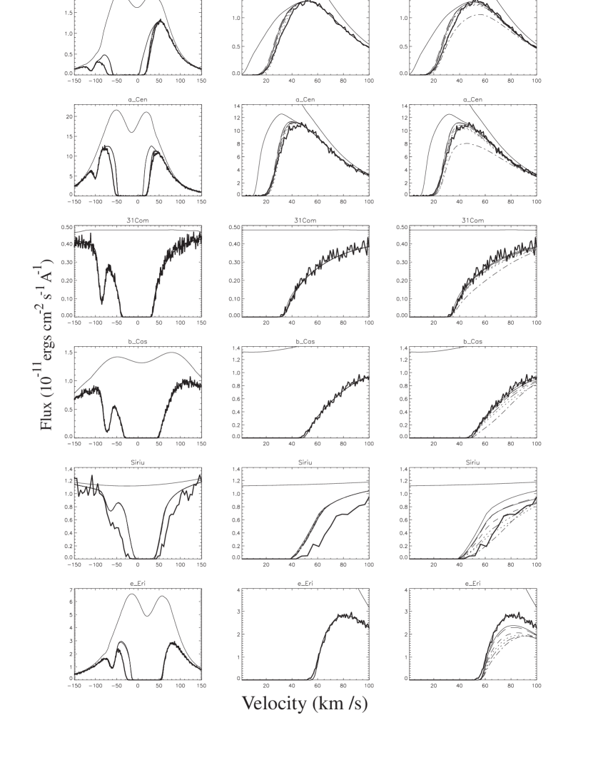
Figure 7: Left column: HST Ly $\alpha$ spectra of six stars: 36 Oph, $\alpha$ Cen, 31 Com, $\beta$ Cas, Sirius, $\epsilon$ Eri, respectively from top to bottom. Each plot shows the observed profile (thick solid line), assumed stellar line profile and interstellar absorption (thin solid lines). Middle column: Reproduction of left column, zoomed in on the red side of Ly-$\alpha$ absorption line. In addition, simulated Ly-$\alpha$ profiles after interstellar and hydrogen wall absorption are shown for models 1-6. Solid lines, when it is different from assumed stellar profile and interstellar absorption, correspond to model 1; dotted lines show results of model 2; dashes correspond to model 3; dot-dash curves correspond to model 4, dot-dot-dot-dash lines correspond to model 5, long dashes correspond to model 6. Right column: same as the middle column, but heliosheath absorption is added to the simulated Ly-$\alpha$ profiles.

5 Comparison of theory and observations

The middle and right columns of Figure 7 show the Ly $\alpha$ lines zoomed in on the red side of the HI absorption line, since that is where most of the heliospheric absorption is expected. The Ly $\alpha$ profile after interstellar absorption is shown in the plots as solid lines. The middle column also shows Ly $\alpha$ profiles after interstellar and hydrogen wall absorption, while the right column shows Ly $\alpha$ profiles after interstellar, hydrogen wall, and heliosheath absorption. The hydrogen wall and heliosheath components are shown for all six models discussed above (see Table 1).

The absorption spectra toward upwind directions (36 Oph and $\alpha$ Cen) are fitted rather well by hydrogen wall absorption only. In comparing the theoretical absorption with data, the most important place for the model to agree with the data is at the base of the absorption, where it is very difficult (if not impossible) to correct any discrepancies by altering the assumed stellar Ly $\alpha$ profile [Wood et al., 2000b]. Toward 36 Oph, model 2 produces slightly more absorption and model 6 produces slightly less absorption at its base compared to the data. For other models the differences between model predictions and HST data at the base can be reduced by small corrections to the assumed stellar profile and interstellar absorption. Toward $\alpha$ Cen, all models show slightly more absorption at the base than the data, except for model 6. It is interesting to note that model 6 fits the $\alpha$ Cen data remarkably well, while it does not fit as well the Ly $\alpha$ spectrum of 36 Oph. Note that these discrepancies with the data just discussed are small enough that they could in principle be corrected by reasonably small changes to the assumed stellar Ly $\alpha$ profile or interstellar absorption, although the better fits in Figure 7 are still to be preferred.

The heliosheath absorption, which is added to the interstellar and hydrogen wall absorption in the right column of Figure 7, does not change the fits much for the upwind lines of sight. Model 2 predicts too much absorption toward both 36 Oph and $\alpha$ Cen and produces the greatest difference with the data at the base of the absorption where it matters most. Consideration of the heliosheath absorption significantly increases the total heliospheric absorption predicted by model 4. The models with the worst agreement in the upwind directions (model 2 and model 4) correspond to the extreme case of small interstellar proton number density, $n_{p,LIC}$.

The observed absorption in the crosswind lines of sight to 31 Com and $\beta$ Cas shows no need for any heliospheric absorption, and our models do not generally predict significant absorption in the crosswind directions that can be clearly distinguished from interstellar absorption. Significant heliosheath absorption in model 4 makes the model the worst fit to the data in the crosswind directions. The other models fit the data acceptably well.

Results of the comparison for downwind lines of sight are more puzzling. It is clearly seen that the missing absorption toward Sirius can be easily explained by absorption in the heliosheath. Moreover, the heliosheath absorption predicted by different models is noticeably different. Model 4, which has the worst fit to the data for all other lines of sight, fits the observed Sirius spectrum better than other models.

In contrast to Sirius, for $\epsilon$ Eri the interstellar absorption fits the observed spectrum very well and there is no need for heliospheric absorption. There is no hydrogen wall absorption in this direction (middle column of Figure 7), but all of our models predict too much heliosheath absorption. A similar problem was also found by Wood et al. [2000b] when they compared their kinetic models with the data. The discrepancy may be even more dramatic than our models suggest, because our computational grid extends only 700 AU in the downwind direction, which as stated above is not far enough to account for all the absorption. A larger grid would presumably make the $\epsilon$ Eri discrepancies worse for all models, and also change which model fits best for Sirius.

6 Discussion

As seen from the previous section, absorption spectra toward five of six stars can be explained by taking into account the hydrogen wall absorption only. Only the Sirius line of sight requires a detectable amount of heliosheath absorption to fit the data. Unfortunately, the hydrogen wall absorption is not very sensitive to such interstellar parameters as the interstellar proton and H atom number densities. The hydrogen wall absorption is most apparent and detectable in upwind directions. The small differences between the models and observations in these directions can be eliminated by small alterations of the stellar profiles (see Figure 7). The poorest agreement is for model 2. After including heliosheath absorption, model 4 seems to predict too much heliosheath absorption compared with the upwind data. Therefore, model 2 and model 4 produce the worst agreement with the data. This conclusion is also consistent with the analysis of absorption in crosswind directions (31 Com, $\beta$ Cas).

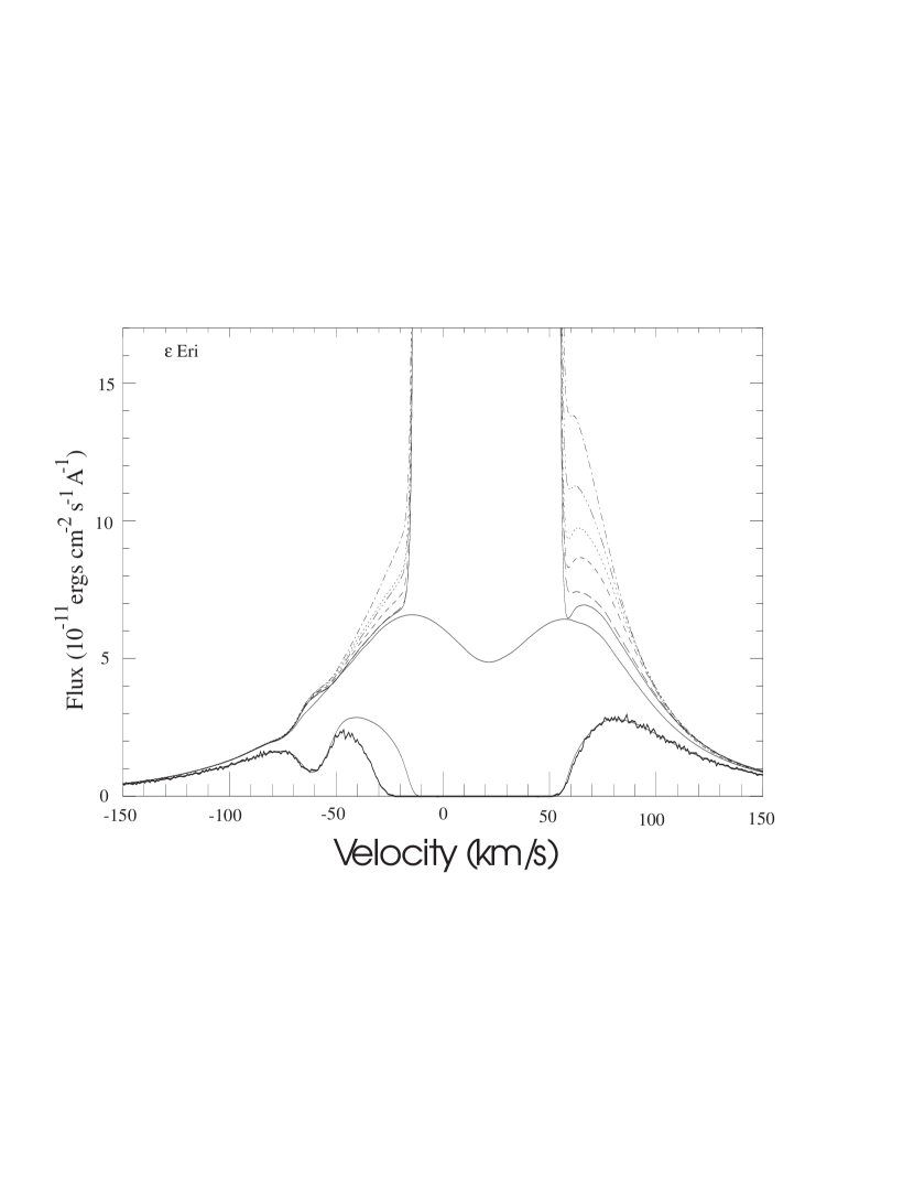
Figure 8: Modifications to the assumed stellar Ly-$\alpha$ profile of $\epsilon$ Eri that lead to better fits to the data for our 6 models. The lines are identified with the models the same as in Figure 7.

Downwind lines of sight (Sirius and $\epsilon$ Eri) can serve as good diagnostics of the heliosheath absorption. For the assumed stellar line profiles, all models predict too much absorption toward the most downwind line of sight, $\epsilon$ Eri. However, since most of the discrepancy is away from the base of the absorption, we can try to correct this problem by modifying the shape of the assumed stellar Ly-$\alpha$ profile. Figure 8 demonstrates how the stellar profile of $\epsilon$ Eri would have to be modified in order to improve agreement with the data. We do not display the central part of the profile, because the absorption is saturated, providing no information on the stellar Ly-$\alpha$ profile there. Because the models predict too much absorption, the fluxes of the assumed stellar profile must be increased to improve the fit.

The revised profiles in Figure 8 are plausible in that they generally do not contain extremely steep slopes or fine structure. However, it is questionable if the tallest of these profiles (for models 4 and 5) are truly realistic. The revised stellar profiles in Figure 8 would suggest that the stellar Ly $\alpha$ profile of $\epsilon$ Eri is significantly taller and narrower than the line profiles of similar stars like $\alpha$ Cen B and 36 Oph (see Figure 7), and the Sun. There is some subjectivity in deciding what is plausible and what is not, but we would conclude from Figure 8 that models 4 and 5 probably require unrealistic modification to the stellar line profile to fit the data, but the other four models that require less extreme alterations of the assumed stellar profile may be all right. In truth, however, the situation is actually worse than this, because as mentioned above our models do not extend far enough downwind and therefore underestimate the amount of heliosheath absorption. Since a larger grid size would significantly worsen agreement with the data, it is uncertain whether any of the six models is truly consistent with the $\epsilon$ Eri data. Furthermore, since the kinetic models presented by Wood et al. [2000b] had the same problem with the $\epsilon$ Eri line of sight, it is possible that inaccuracies in the physical assumptions involved in current kinetic models may be resulting in overpredictions of absorption in downwind directions, although additional theoretical work is required to test this interpretation.

The models that have the least disagreement with the $\epsilon$ Eri line of sight are models 1 and 6. The common feature of these models is that both predict small number densities of H atoms of population 2. In model 1 this is due to a low assumed interstellar H density, while in model 6 this is due to the small size of the heliosheath. Model 6 in fact predicts the narrowest heliosheath region of our six models. However, the interstellar proton and H atom number densities of this model seem to be unrealistically high, because the model predicts that the termination shock should be at 70 AU in the upwind direction. As of August 2001, Voyager 1 was at 82 AU and Voyager 2 was at $\sim$65 AU, and neither has yet encountered the termination shock. Due to its low assumed interstellar H density, model 1 predicts the smallest amount of H atoms penetrating through the heliopause into the heliosphere of our six models. The number density of H atoms at the termination shock is 0.056 cm^-3 for this model. This value is very close to the number density derived from the observed deceleration of the solar wind due to interaction with interstellar H atoms. Comparison of the solar wind speed measured on Ulysses and Voyager shows a decrease of about 40 km s^-1, or 10% in radial speed near 60 AU. Wang and Richardson [2001] have shown that this speed decrease implies an interstellar neutral density at the termination shock of 0.05 cm^-3, which is close to our model 1 value.

Consideration of the Sirius line of sight complicates matters further. Model 2 and especially model 4 fit the observed profile very well, once again focusing our attention at the base of the absorption (see Figure 7), while the other models predict too little absorption. Models 2 and 4 assume a small interstellar ionization fraction in the vicinity of Sun, and recent studies of the LIC ionization state are in favor of such small ionization [Lallement, 1999]. However, model 4 does not fit the other lines of sight well, and it must be noted once again that the models will underestimate the amount of heliosheath absorption in downwind directions due to the limited extent of the current model grid.

The Ly-$\alpha$ absorption profile of the Sirius spectrum has been a controversial subject for the last few years and will probably remain so. First interpreted as due to absorption by a stellar wind from Sirius A [Bertin et al., 1995a], the extra absorption on the blue side of the line has later been explained as resulting from an astrosphere around Sirius and shown to be compatible with a very crude model of such an astrosphere. However, the comparison between the Sirius B and Sirius A spectra later obtained by Hebrard et al. [1999] has shown that a large fraction (if not the totality) of the extra absorption is specific to Sirius A and must arise closer to the star than predicted by an astrospheric model, favoring again a stellar wind as the source of the absorption. On the other hand, the extra absorption on the red side, first interpreted as due to interstellar hot gas [Bertin et al., 1995b], has later been compared satisfactorily with heliospheric absorption by the heliosheath [Izmodenov et al., 1999], an interpretation which appears plausible based on Figure 7. Unfortunately, the comparison with Sirius B does not help here to disentangle the sources of the absorption, since the Sirius B spectrum shows a broader and deeper absorption on the red wing, which encompasses the Sirius A line, and is identified by Hebrard et al. [1999] as due to the intrinsic photospheric Ly-$\alpha$ profile. Hebrard et al. [1999] also note that the excess absorption on the red side of the line can be removed if one relaxes the assumption that both interstellar components detected toward Sirius have ${\rm D/H}=1.6\times 10^{-5}$. The heliosheath or interstellar gas remain possible sources for the excess absorption seen towards Sirius A on the red side of the line. If the absorption is due to the heliosheath, this is the only line of sight in which heliosheath absorption is detected.

We now suggest one possible cause of our difficulties with downwind lines of sight. The process of pickup ion assimilation into the solar wind is a very complicated phenomenon. Currently, it is believed that pickup ions form a separate population of protons, which is co-moving with the solar wind proton plasma. The process of energy exchange between the populations is quite slow and it is expected that the relaxation time is large compared with the time that is needed for a proton to reach the termination shock distance. How the non-equilibrium distribution of pickup ions is affected by the termination shock is still an open question, although some scenarios have been developed [e.g., Fichtner, 2001]. Our model considers the solar protons and pickup ion protons as one fluid. This approach is based on fundamental questions of mass, momentum, and energy conservation. Therefore, it is quite natural to expect that the model predicts the positions of the shocks and the heliopause reasonably well. At the same time, measurements of speed and temperature of the solar wind at large heliocentric distances by Voyager are in favor of the two populations being co-moving, but thermally different. This suggests a different scenario of the heliosheath plasma flow than is assumed in our model.

This new scenario would result in different distributions of H atoms created in the heliosheath, which could possibly solve our difficulties in modeling the heliospheric absorption in downwind directions. A priori, we cannot exclude a scenario that provides the greatest absorption at heliocentric angles of about $130-150^{\circ}$ from upwind. For such a scenario, perhaps all six lines of sight in Figure 7 could be explained simultaneously. Calculating energetic neutral atom (ENAs) fluxes, Gruntman et al. [2001] consider different plasma scenarios of heliosheath plasma flow. One of the models considered in the paper suggests a maximum of ENA fluxes in directions of $130-150^{\circ}$ from upwind. This model assumes that the pickup proton population is carried through the shock without thermalization, i.e., preserving its velocity distribution filling the sphere in velocity space. Since ENAs originate in the heliosheath, it supports the idea to consider different scenarios of the heliosheath plasma in order to interpret all six observable spectra simultaneously. It remains to be seen whether such models could both reproduce the absorption seen toward Sirius and solve our problem of overpredicting absorption toward $\epsilon$ Eri.

Finally, we have to note that an axisymmetric model of the heliospheric interface was used to calculate the heliospheric absorption. The actual heliosphere is not axisymmetric due to both the latitudinal variation of the solar wind and possible effects of the interstellar magnetic field. Note, however, that the upwind direction of the ISM flow is only about $8^{\circ}$ from the ecliptic, so variations of solar wind properties with latitude are unlikely to produce major differences from the axisymmetric approximation. In any case, asymmetry in the heliosheath or hydrogen wall could result in the heliospheric absorption being different from axisymmetric. A 3D model is needed to assess the inaccuracies introduced by the axisymmetric assumption, but unfortunately there is as yet no adequate 3D model including the interstellar H atom population that can address this issue. Such a model is currently being developed by us.

At the same time, our results can be interpreted as indirect evidence that there is no strong deviation of the heliospheric interface from being axisymmetric, since all four upwind/crosswind lines of sight discussed here can be well interpreted on the base of axisymmetric model. Taking into account the discussion above, one may conclude that our difficulties with the downwind lines of sight have other interpretations. However, this statement needs to be verified by 3D modeling of the heliospheric interface and by studying the sensitivity of heliospheric absorption to the 3D structure.

7 Summary

We have compared H I Ly-$\alpha$ absorption profiles toward six nearby stars observed by HST with theoretical profiles computed using Baranov-Malama model of the heliospheric interface with six different sets of model parameters. Our results are summarized as follows:

1. It has been shown that the absorption produced by the hydrogen wall does not depend significantly on local interstellar H atom and proton number densities for upwind and crosswind directions. In downwind directions the hydrogen wall absorption is sensitive to interstellar densities, but this absorption component is most easily detected in upwind directions. In crosswind and downwind directions the hydrogen wall absorption is hidden in the saturated interstellar absorption and cannot be observed.

2. The heliosheath absorption varies significantly with interstellar proton and H atom number densities. For all models, the heliosheath absorption is more pronounced in crosswind and downwind directions. The heliosheath absorption is redshifted in crosswind directions compared with the interstellar and hydrogen wall absorption components.

3. Comparison of computations and data shows that all available absorption spectra, except that of Sirius, can be explained by taking into account the hydrogen wall absorption only. Considering heliosheath absorption, we find that all models have a tendency to overpredict heliosheath absorption in downwind directions. Toward upwind and crosswind stars the small differences between model predictions and the data can be corrected by small alterations of the assumed stellar Ly-$\alpha$ profile. However, the downwind $\epsilon$ Eri line of sight is a problem, as the models predict too much heliosheath absorption in that direction, and for many, if not most, of the models the discrepancy with the data is too great to resolve by reasonable alterations of the stellar profile.

4. It is puzzling that model 4 provides the best fit to the absorption profile toward Sirius but the worst fit to the other lines of sight. This may be due to our models underestimating heliosheath absorption in downwind directions due to limited grid size, or perhaps the detected excess absorption toward Sirius is not really heliospheric in origin, as suggested by previous authors. It is also possible that the difficulties the models have with the downwind lines of sight towards Sirius and $\epsilon$ Eri might be resolved by modifications to the models, perhaps by taking into account the multi-component nature of the heliosheath plasma flow.