Cosmological dark matter annihilations into $\gamma$-rays – a closer look

Abstract

We investigate the prospects of detecting weakly interacting massive particle (WIMP) dark matter by measuring the contribution to the extragalactic gamma-ray radiation induced, in any dark matter halo and at all redshifts, by WIMP pair annihilations into high-energy photons. We perform a detailed analysis of the very distinctive spectral features of this signal, recently proposed in a short letter by three of the authors: The gamma-ray flux which arises from the decay of $\pi^{0}$ mesons produced in the fragmentation of annihilation final states shows a severe cutoff close to the value of the WIMP mass. An even more spectacular signature appears for the monochromatic gamma-ray components, generated by WIMP annihilations into two-body final states containing a photon: the combined effect of cosmological redshift and absorption along the line of sight produces sharp bumps, peaked at the rest frame energy of the lines and asymmetrically smeared to lower energies. The level of the flux depends both on the particle physics scenario for WIMP dark matter (we consider, as our template case, the lightest supersymmetric particle in a few supersymmetry breaking schemes), and on the question of how dark matter clusters. Uncertainties introduced by the latter are thoroughly discussed implementing a realistic model inspired by results of the state-of-the-art N-body simulations and semi-analytic modeling in the cold dark matter structure formation theory. We also address the question of the potential gamma-ray background originating from active galaxies, presenting a novel calculation and critically discussing the assumptions involved and the induced uncertainties. Furthermore, we apply a realistic model for the absorption of gamma-rays on the optical and near-IR intergalactic radiation field to derive predictions for both the signal and background. Comparing the two, we find that there are viable configurations, in the combined parameter space defined by the particle physics setup and the structure formation scenario, for which the WIMP induced extragalactic gamma-ray signal will be detectable in the new generation of gamma-ray telescopes such as GLAST.

I Introduction

The accumulated evidence for the existence of large amounts of nonbaryonic dark matter in the Universe is by now compelling (for a review, see e.g. lbreview ). Data on the cosmic microwave background (CMB)cmbr and supernova observations supernovae jointly fix the energy fraction in the form matter and cosmological constant (or something similar) to $\Omega_{M}\sim 0.3$ and $\Omega_{\Lambda}\sim 0.7$, respectively. At the same time, the CMB measurements limit the contribution from ordinary baryons to less than $\Omega_{B}\sim 0.05$, which is in excellent agreement with big bang nucleosynthesis. This means that non-baryonic matter has to make up most of the matter in the Universe, $\Omega_{DM}\simeq\Omega_{M}$. Incidentally, recent measurements of the large-scale distribution of galaxies independently confirm $\Omega_{M}=0.27\pm 0.06$ licia , giving further credence to these conclusions. The currently best estimate of $\Omega_{M}$ comes from a joint analysis of CMB and large scale structure data 2dF and gives $\Omega_{M}h^{2}=0.115\pm 0.009$ where $h$ is the Hubble constant in units of 100 km s^-1 Mpc^-1.

When it comes to the question of how the dark matter is distributed on small, galactic and sub-galactic, scales the situation is much less clear, however (for a review, see, e.g., moorerev ). After being subject to an extensive debate, with both theoretical and observational controversies, it seems that the Cold Dark Matter (CDM) model, with dark matter made of, e.g., weakly interacting massive particles (WIMPs), or the $\Lambda$CDM model, with a contribution from the cosmological constant, are in fair agreement with current observations, so that drastic modifications like strong self-interaction are not urgently called for (see, e.g., primack ).

Focusing on the CDM model with WIMPs as dark matter candidates, there is an obvious interest to use as much as possible of the knowledge of the distribution of CDM given through state-of-the-art N-body simulations. In particular, the distribution of dark matter plays a crucial role in most WIMP detection methods, and determines therefore the possibility of identifying the dark matter and pinning down its particle properties.

In this vein, we recently presented a short note beu (hereafter BEU) where, contrary to previous predictions previous , it was shown that in the hierarchical picture found in CDM simulations the cosmic $\gamma$-ray signal from WIMP annihilations may be at the level of current estimates of the extragalactic $\gamma$-ray flux. In this paper we deal more carefully with the issues of the formation of structure in a CDM or, rather, $\Lambda$CDM universe, investigating the sensitivity of the expected gamma-ray flux to different treatments of the structure formation process. We also address the question of the diffuse background flux expected from various types of active galaxies and compare its spectral features with those of the signal from WIMP annihilations. We consider several sample cases in a theoretically favored WIMP scenario, that of supersymmetric dark matter, and highlight the possibility to disentangle such signals from the background in future measurements of the the extragalactic $\gamma$-ray flux, in particular with the GLAST detector. Results for both the signal and background components are presented implementing a careful treatment of the absorption of high energy gamma-rays in the intergalactic space caused by pair production on the optical and infrared photon background.

The paper is organized as follows. In Sec. II we set up the general formalism for computing the dark matter induced gamma-ray flux. In Sec. III we investigate the properties of dark matter halos, on all scales of relevance to our problem, in various semi-analytical and numerical simulation scenarios. Implications for the WIMP induced gamma-ray flux are discussed in Sec. IV, while in Sec. V, we investigate the background problem, including the effects of varying within present observational limits the slope of the energy spectrum of the gamma-ray emission from active galaxies. We also check the effects of removing some more resolved point sources, as may be expected for the next generation of experiments. In Sec. VI we show a few examples of what signals can be expected for one of the favored WIMP candidates, the neutralino, and give an estimate of sensitivity curves for the GLAST detector. Sec. VII contains our conclusions.

II The dark matter induced extragalactic gamma-ray flux

There are several ways to compute the gamma-ray flux generated in unresolved cosmological dark matter sources. In BEU the result was derived by tracing the depletion of dark matter particles with the Boltzmann equation. The approach we describe here, in which we simply perform a sum of contributions along a given line of sight (or better, a given geodesic), gives the same result but shows more directly the role played by structure in the Universe. We assume a standard homogeneous and isotropic cosmology, described by the metric:

$$ds^{2}=c^{2}dt^{2}-R^{2}(t)\left[dr^{2}+S_{k}^{2}(r)d\Omega^{2}\right]\;,$$ (1)

where $d\Omega^{2}=d\theta^{2}+\sin^{2}\theta d\phi^{2}$ and where the function $S_{k}(r)$ depends on the overall curvature of the Universe:

$$S_{k}(r)=\cases{r,&$k=0$;\cr\arcsin r,&$k=+1$;\cr{\rm arsinh}r,&$k=-1$.}$$ (2)

In our applications, we will safely use $k=0$ (i.e.  we assume a flat geometry for the Universe). The angular interval $d\Omega=\sin\theta d\theta d\phi$ may, e.g., correspond to the angular acceptance of a given detector. At redshift $z$, $d\Omega$ and the radial increment $dr$ determine the proper volume:

$$dV=\frac{[R_{0}S_{k}(r)]^{2}\,R_{0}}{(1+z)^{3}}drd\Omega\;.$$ (3)

Let $d{\cal N}_{\gamma}/dE(E,M,z)$ be, on average, the differential energy spectrum for the number of $\gamma$-rays emitted, per unit of time, in a generic halo of mass $M$ located at redshift $z$. Even for large $M$, this source can be safely regarded as point-like and unresolved (with the upcoming generation of gamma-ray telescopes, it might be possible to resolve the dark-matter induced flux from galaxies in the local group, but almost certainly not further out). Summing over all such sources present in $dV$, we can find the number of photons emitted in this volume and, say, in the time interval $dt$ and energy range $(E,\,E+dE)$; the emission process being isotropic, the corresponding number of photons $dN_{\gamma}$ collected by a detector on earth with effective area $dA$ during the time $dt_{0}$ and in the (redshifted) energy range $(E_{0},\,E_{0}+dE_{0})$, is equal to:

$$dN_{\gamma}=e^{-\tau(z,E_{0})}\left[(1+z)^{3}\,\int dM\;\frac{dn}{dM}(M,z)\,\frac{d{\cal N}_{\gamma}}{dE}\left(E,M,z\right)\right]\;\frac{dV\,dA}{4\pi[R_{0}S_{k}(r)]^{2}}\,dE_{0}\,dt_{0}\;,$$ (4)

where we applied the relation $dt\,dE=(1+z)^{-1}dt_{0}\,(1+z)dE_{0}=dt_{0}\,dE_{0}$, and we introduced the halo mass function $dn/dM$, i.e. the comoving number density of bound objects that have mass $M$ at redshift $z$ (the factor $(1+z)^{3}$ converts from comoving to proper volume). The first factor in Eq. (4) is an attenuation factor which accounts for the absorption of $\gamma$-rays as they propagate from the source to the detector: the main effect for GeV to TeV $\gamma$-rays is absorption via pair production on the extragalactic background light emitted by galaxies in the optical and infrared range. Detailed studies of this effect, involving a modeling of galaxy and star formation and a comparison with data on the extragalactic background light, have been performed by several groups (see, e.g., abs1 ; abs2 ; SaSt98 ; deJaSt02 ; abs4 ; abs ). We take advantage of the results recently presented by the Santa Cruz group abs ; we implement an analytic parameterization of the optical depth $\tau$, as a function of both redshift and observed energy, which reproduces within about 10% the values for this quantity plotted in Figs. 5 and 7 in Ref. abs ($\Lambda$CDM model labelled “Kennicut”; the accuracy of the parameterization is much better than the spread in the predictions considering alternative models abs ). For comparison, we have verified that the results presented in Salamon and Stecker SaSt98 (their model in Fig. 6, with metallicity correction) is in fair agreement with the model we are assuming as a reference model in the energy range of interest in this work, i.e. below a few hundred GeV.

The estimate of the diffuse extragalactic $\gamma$-ray flux due to the annihilation of dark matter particles is then obtained by summing over all contributions in the form in Eq. (4):

$$\frac{d\phi_{\gamma}}{dE_{0}}\equiv\frac{dN_{\gamma}}{dA\,d\Omega\,dt_{0}\,dE_{0}} = \frac{1}{4\pi}\int dr\,R_{0}e^{-\tau(z,E_{0})}\int dM\;\frac{dn}{dM}(M,z)\,\frac{d{\cal N}_{\gamma}}{dE}\left(E_{0}\,(1+z),M,z\right)$$ (5)

$$= \frac{c}{4\pi}\int dz\frac{e^{-\tau(z,E_{0})}}{H_{0}\,h(z)}\int dM\;\frac{dn}{dM}(M,z)\,\frac{d{\cal N}_{\gamma}}{dE}\left(E_{0}\,(1+z),M,z\right)\;.$$

where the integration along the line of sight has been replaced by one over redshift, $H_{0}$ is the Hubble parameter, $c$ is the speed of light and $h$ depends on the cosmological model,

$$h(z)=\sqrt{\Omega_{M}(1+z)^{3}+\Omega_{K}(1+z)^{2}+\Omega_{\Lambda}}.$$ (6)

In this work we put the contribution from curvature $\Omega_{K}=0$, in agreement with the prediction from inflation and with recent measurements of the microwave background cmbr . Taking the limit in which all structure is erased and dark matter is smoothly distributed at all redshifts, Eq. (5) correctly reduces to the analogous formula derived with the Boltzmann equation in BEU (Eq. (4) therein).

III The properties of halos

Three ingredients are needed to use Eq. (5) for an actual prediction of the $\gamma$-ray flux. We need to specify the WIMP pair annihilation cross section and estimate the number of photons emitted per annihilation, as well as the energy distribution of these photons: the choice of the particle physics model fixes this element. As photons are emitted in the annihilation of two WIMPs, the flux from each source will scale with the square of the WIMP number density in the source. The second element needed is then the dark matter density profile in a generic halo of mass $M$ at redshift $z$. Finally we need to know the distribution of sources, i.e. we need an estimate of the halo mass function.

Some insight on the latter two ingredients comes from the $\Lambda$CDM model for structure formation: we outline here hypotheses and results entering the prediction for the dark matter induced flux. We start with the mass function for dark matter halos.

III.1 The halo mass function

Press-Schechter PreSch theory postulates that the cosmological mass function of dark matter halos can be cast into the universal form:

$$\frac{dn}{dM}=\frac{\bar{\rho}_{0}}{M^{2}}\nu f(\nu)\frac{d\,log\nu}{d\,logM}$$ (7)

where $\bar{\rho}_{0}$ is the comoving dark matter background density, $\bar{\rho}_{0}\simeq\rho_{c}\Omega_{M}$ with $\rho_{c}$ being the critical density at $z=0$. We introduced also the parameter $\nu\equiv\delta_{sc}(z)/\sigma(M)$, defined as the ratio between the critical overdensity required for collapse in the spherical model $\delta_{sc}$ and the quantity $\sigma(M)$, which is the present, linear theory, rms density fluctuation in spheres containing a mean mass $M$. An expression for $\delta_{sc}$ is given, e.g., in Ref. ECF . $\sigma(M)$ is related to the fluctuation power spectrum $P(k)$, see e.g. Ref. Peebles , by:

$$\sigma^{2}(M)\equiv\int d^{3}k\;\tilde{W}^{2}(k\,R)\,P(k)$$ (8)

where $\tilde{W}$ is the top-hat window function on the scale $R^{3}=3M/4\pi\bar{\rho}$ with $\bar{\rho}$ the mean (proper) matter density. The power spectrum is parametrized as $P(k)\propto k^{n}T^{2}(k)$; we fix the spectral index $n=1$ and take the transfer function $T$ as given in the fit by Bardeen et al. Bardeenetal for an adiabatic CDM model, with the shape parameter modified to include baryonic matter according to the prescription in, e.g. Peacock , Eq. (15.84) and (15.85). Note that the fit we use agrees within 10% with the analytic result obtained for large $k$ in Ref. HUSU , hence holds to the accuracy we are concerned about for the small scales we will consider below. We normalize $P$ and $\sigma$ by computing $\sigma$ in spheres of $R=8/h$ Mpc and setting the result equal to the parameter $\sigma_{8}$ ($h$ is the usual Hubble constant in units of 100 km s^-1 Mpc^-1).

In Eq. (7) $f(\nu)$ is known as the multiplicity function; we implement the form found in the ellipsoidal collapse model SMT :

$$\nu f(\nu)=2A\left(1+\frac{1}{\nu^{\prime 2q}}\right)\left(\frac{\nu^{\prime 2}}{2\pi}\right)^{1/2}\exp\left(-\frac{\nu^{\prime 2}}{2}\right)$$ (9)

where $\nu^{\prime}=\sqrt{a}\nu$, and the parameters $q=0.3$ and $a=0.707$ are derived by fitting Eq. (7) to the N-body simulation results of the Virgo consortium virgo , while $A$ is fixed by the requirement that all mass lies in a given halo, i.e. $\int d\nu f(\nu)=1$ or $\int dM\;Mdn/dM=\bar{\rho}_{0}$. Eq. (9) reduces to the form originally proposed in Press-Schechter theory and valid for spherical collapse if $a=1$, $q=0$ and $A=0.5$.

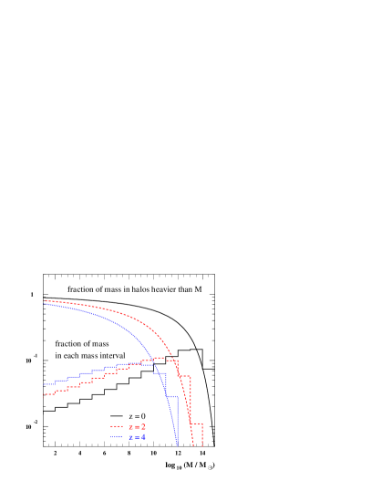
Figure 1: Fraction of total mass provided by objects heavier than a given mass $M$ (upper curves) or within 14 decades in mass (lower histograms) at three different redshifts and for the mass function as derived in the ellipsoidal collapse model.

To give the reader a feeling for what the distribution of mass is, as predicted by the halo mass function we are considering here, in Fig. 1 we plot the fraction of the total mass in halos heavier than $M$, and the fraction per mass decade, for three different redshifts, $z$ equal to 0, 2 and 4, and for our default choice of cosmological model: $\Omega_{M}=0.3$, $\Omega_{\Lambda}=0.7$, $h=0.7$, $\Omega_{b}=0.022/h^{2}$ and $\sigma_{8}=0.73$ 2df . Note the peak in the distribution at $M\sim 10^{12}-10^{13}\,M_{\odot}{\ }$ for $z=0$ rapidly moving to lower masses for larger redshifts; note also that the low mass tails are not very steep, with only 89% (81%) of the total mass in structures heavier than $10\,M_{\odot}{\ }$ at $z=0$ ($z=2$). These numbers get slightly larger if one applies the spherical collapse model instead of the ellipsoidal model we have considered here.

III.2 The density profile in dark halos

In the $\Lambda$CDM model for structure formation, dark matter halos are assumed to form hierarchically bottom-up via gravitational amplification of initial density fluctuations. Small structures merge into larger and larger halos and final configurations are self-similar, with a smooth dark matter component and, possibly, a small fraction of the total mass in subhalos which have survived tidal stripping. We neglect for the moment eventual substructure, whose role on the WIMP induced signal is discussed in the next Section. N-body simulations seem to indicate that dark matter density profiles can be described in the form

$$\rho(r)=\rho^{\prime}\,g(r/a)\;,$$ (10)

where $a$ is a length scale and $\rho^{\prime}$ the corresponding density. The function $g(x)$ is found to be more or less universal over the whole mass range of the simulated halos, although different functional forms have been claimed in different simulations: we will consider the result originally proposed by Navarro, Frenk and White NFW (hereafter NFW profile),

$$g_{\rm NFW}\left(x\right)={1\over x\left(1+x\right)^{2}},$$ (11)

supported also by more recent simulations performed by the same group nfwnew , and the result found in the higher resolution simulation (but with fewer simulated halos) by Moore et al. moore (hereafter Moore profile),

$$g_{\rm Moore}\left(x\right)={1\over x^{1.5}\left(1+x^{1.5}\right)}.$$ (12)

The two functional forms have the same behavior at large radii and they are both singular towards the center of the halo, but the Moore profile increases much faster than the NFW profile (non-universal forms, with central cusp slopes depending on evolution details have been claimed as well klypin ). There have been a number of reports in the literature arguing that the rotation curves of many small-size disk galaxies rule out divergent dark matter profiles, see, e.g., FP ; moorerot (note however that this issue is not settled yet, see, e.g., VDB ), while they can be fitted by profiles with a flat density core. We consider then here as a third alternative functional form the Burkert profile Burkert ,

$$g_{\rm B}\left(x\right)={1\over\left(1+x\right)\left(1+x^{2}\right)},$$ (13)

which has been shown to be adequate to reproduce a large catalogue of rotation curves of spiral galaxies BS .

Rather than by $a$ and $\rho^{\prime}$, it is useful to label a dark matter profile by its virial mass $M$ and concentration parameter $c_{vir}$. For the latter, we adopt here the definition by Bullock et al. Bullock : let the virial radius $R_{vir}$ of a halo of mass $M$ at redshift $z$ be defined as the radius within which the mean density of the halo is $\Delta_{vir}$ times the mean background density $\bar{\rho}(z)$ at that redshift:

$$M\equiv{4\pi\over 3}\Delta_{vir}\bar{\rho}(z)\,R_{vir}^{3}.$$ (14)

We take the virial overdensity to be approximated by the expression BN , valid in a flat cosmology,

$$\Delta_{vir}\simeq{(18\pi^{2}+82x-39x^{2})\over\Omega_{M}(z)}$$ (15)

with $x\equiv\Omega_{M}(z)-1$, ($\Delta_{vir}\simeq 337$ for $\Omega_{M}=0.3$ at $z=0$). The concentration parameter is then defined as

$$c_{vir}=\frac{R_{vir}}{r_{-2}}$$ (16)

with $r_{-2}$ the radius at which the effective logarithmic slope of the profile is $-2$, i.e. it is the radius set by the equation $d/dr\left.\left(r^{2}g(r)\right)\right|_{r=r_{-2}}=0$. This means that $r_{-2}=a$ for the NFW profile, while $x_{-2}\equiv r_{-2}/a$ is equal to about 0.63 for the Moore profile and to 1.52 for the Burkert profile. Note that these definitions of $R_{vir}$ and $c_{vir}$ differ from those adopted in Ref. NFW and Ref. ENS .

After identifying the behavior in Eq. (10), Navarro et al. noticed also that, for a given cosmology, the halos in their simulation at a given redshift show a strong correlation between $c_{vir}$ and $M$ NFW , with larger concentrations in lighter halos. This trend may be intuitively explained by the fact that low-mass halos typically collapsed earlier, when the Universe was denser. Bullock et al. Bullock confirmed this behavior with a larger sample of simulated halos and propose a toy model to describe it, which improves on the toy model originally outlined in NFW : On average, a collapse redshift $z_{c}$ is assigned to each halo of mass $M$ at the epoch $z$ through the relation $M_{\star}(z_{c})\equiv FM$, where the typical collapsing mass $M_{\star}$ is defined implicitly by $\sigma\left(M_{\star}(z)\right)=\delta_{sc}(z)$ and is postulated to be a fixed fraction $F$ of $M$ (following Ref. Wechsleretal we choose $F=0.015$). The density of the Universe at $z_{c}$ is then associated with a characteristic density of the halo at $z$; it follows that, on average, the concentration parameter is given by:

$$c_{vir}(M,z)=K\frac{1+z_{c}}{1+z}=\frac{c_{vir}(M,z=0)}{(1+z)}$$ (17)

where $K$ is a constant (i.e. independent of $M$ and cosmology) to be fitted to the results of the simulations. Bullock et al. Bullock show that this toy model reproduces rather accurately the dependence of $c_{vir}$ found in the simulations on both $M$ and $z$. We reproduce this fit at $z=0$ in Fig. 2 (left panel, solid line); “data” points and relative error bars are taken from Bullock and just represent a binning in mass of results in their simulated halos: in each mass bin, the marker and the error bars correspond, respectively, to the peak and the 68% width in the $c_{vir}$ distribution. We determine $K$ with a best fitting procedure in the cosmology $\Omega_{M}=0.3$, $\Omega_{\Lambda}=0.7$, $h=0.7$ and $\sigma_{8}=1$ adopted in the N-body simulation referred to, and then use this value to estimate the mean $c_{vir}$ in other cosmologies; we find $K=4.4$. Finally, following again Bullock et al. Bullock , we assume that, for a given $M$, the distribution of concentration parameters ${\cal{P}}$ is log-normal with a $1\sigma$ deviation $\Delta(\log_{10}c_{vir})$ around the mean, independent of $M$ and cosmology; we take $\Delta(\log_{10}c_{vir})=0.2$.

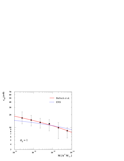
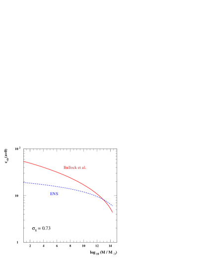
Figure 2: Concentration parameter versus mass for halos of mass $M$ at $z=0$. On the left-hand panel we reproduce from Ref. Bullock the behavior found in a large sample of simulated halos, with a binning in mass in which each marker represents the peak in the distribution and the relative bar its 68% width; the trend is reproduced with the toy models proposed in Ref. Bullock itself (Bullock et al.) and in Ref. ENS (ENS). On the right-hand side, we show an extrapolation of $c_{vir}$ to the whole mass range we need to include in our analysis according to the two toy models.

An alternative toy-model to describe the relation between $c_{vir}$ and $M$ has been discussed by Eke, Navarro and Steinmetz ENS (hereafter ENS model): The relation they propose has a similar scaling in $z$, with however a different definition of the collapse redshift $z_{c}$ and a milder dependence of $c_{vir}$ on $M$. In our notation, they define of $z_{c}$ through the equation:

$$D(z_{c})\sigma_{\rm eff}(M_{p})={1\over C_{\sigma}}$$ (18)

where $D(z)$ represents the linear theory growth factor, and $\sigma_{\rm eff}$ is an ‘effective’ amplitude of the power spectrum on scale $M$:

$$\sigma_{\rm eff}(M)=\sigma(M)\,\left(-\frac{d\ln(\sigma)}{d\ln(M)}(M)\right)=-\frac{d\sigma}{dM}M$$ (19)

which modulates $\sigma(M)$ and makes $z_{c}$ dependent on both the amplitude and the shape of the power spectrum, rather than just on the amplitude as in the toy model of Bullock et al. Finally, in Eq. (18), $M_{p}$ is assumed to be the mass of the halo contained within the radius at which the circular velocity reaches its maximum, while $C_{\sigma}$ is the parameter (independent on $M$ and cosmology) which has to be fitted to the simulations. With this definition of $z_{c}$ it follows that, on average, $c_{vir}$ can be be expressed as:

$$c_{vir}(M,z)=\left(\frac{\Delta_{vir}(z_{c})\,\Omega_{M}(z)}{\Delta_{vir}(z)\,\Omega_{M}(z_{c})}\right)^{1/3}\frac{1+z_{c}}{1+z}\;.$$ (20)

As we already mentioned the dependence of $c_{vir}$ on $M$ as given in the equation above is weaker than in the Bullock et al. toy-model. Our best fitting procedure gives $C_{\sigma}=76$ and the behavior in Fig. 2 (left panel, dashed line), which reproduces the N-body “data” fairly well, with values not very far from those obtained in the Bullock et al. model within the range of simulated masses, and possibly just a slight underestimate of the mean value in the lighter mass end.

On the other hand, the extrapolation outside the simulated mass range can give much larger discrepancies as shown in the right panel of Fig. 2. Solid lines are for the same models as those shown in the left panel ($K$ and $C_{\sigma}$ from the data fit in the left panel), with just $\sigma_{8}$ set equal to our preferred value, $\sigma_{8}=0.73$. When going to small $M$, $c_{vir}$ increases in both cases, but the growth in the model of Bullock et al. is much faster than in the ENS model; we will show explicitly how this uncertainty propagates to the prediction of the dark matter induced $\gamma$-ray flux. The sensitivity of our results to the choice of cosmological parameters is generally much weaker: The largest effect is given by the overall linear scaling of $c_{vir}(M,z)$ with $\sigma_{8}$. There is also the possibility to change the cosmological model by including other dark components; we are not going to discuss any such case in detail, we just mention that a neutrino component at the level of current upper limits is not going to change severely our picture, while a substantial warm dark matter component may play a crucial role if $z_{c}$ is indeed defined according to the ENS prescription.

IV WIMP induced flux: role of structures and spectral features

We are now ready to write explicitly the term $d{\cal N}_{\gamma}/dE$ introduced above and to derive the formula for the flux. The differential energy spectrum for the number of photons emitted inside a halo with mass $M$ at redshift $z$ is

$$\frac{d{\cal N}_{\gamma}}{dE}(E,M,z) = \frac{\sigma v}{2}\frac{dN_{\gamma}(E)}{dE}\int dc^{\,\prime}_{vir}\;{\cal{P}}(c^{\,\prime}_{vir})\left(\frac{\rho^{\prime}}{M_{\chi}}\right)^{2}\int d^{3}r\;g^{2}(r/a)$$ (21)

$$= \frac{\sigma v}{2}\frac{dN_{\gamma}(E)}{dE}\frac{M}{M_{\chi}^{2}}\,\frac{\Delta_{vir}\bar{\rho}}{3}\,\int dc^{\,\prime}_{vir}\;{\cal{P}}(c^{\,\prime}_{vir})\frac{(c^{\,\prime}_{vir}\,x_{-2})^{3}}{\left[I_{1}(c^{\,\prime}_{vir}\,x_{-2})\right]^{2}}\,I_{2}(x_{min},c^{\,\prime}_{vir}\,x_{-2})$$

where $\sigma v$ is the WIMP annihilation rate, $dN_{\gamma}(E)/dE$ is the differential gamma-ray yield per annihilation and $M_{\chi}$ is the WIMP mass. Note that in previous literature, the prefactor $\sigma v/2$ has often been erroneously taken as $\sigma v$. The derivation based on the Boltzmann equation in BEU adds to our confidence that the factor should be $\sigma v/2$. In Eq. (21) we applied the definition of $R_{vir}$ and introduced the integrals

$$I_{n}(x_{min},x_{max})=\int_{x_{min}}^{x_{max}}dx\,x^{2}g^{n}(x)\;.$$ (22)

with the lower limit of integration $x_{min}=r_{min}/a$ set, in a singular halo profile, by WIMP self annihilations, i.e. roughly by $\rho(r_{min})\simeq m_{\chi}/[\sigma v\;(t_{0}-t_{c})]$, where $t_{0}$ is the age of the Universe and $t_{c}$ is the collapse time for the halo under investigation. To include all sources labeled by their mass $M$, we averaged over the log-normal distribution ${\cal{P}}(c^{\,\prime}_{vir})$ centered on $c_{vir}$ as given in Eq. (17) or (20).

Inserting Eq. (21) into Eq. (5), we find that the gamma-ray flux is

$$\frac{d\phi_{\gamma}}{dE_{0}}=\frac{\sigma v}{8\pi}\frac{c}{H_{0}}\frac{\bar{\rho}_{0}^{2}}{M_{\chi}^{2}}\int dz\;(1+z)^{3}\frac{\Delta^{2}(z)}{h(z)}\frac{dN_{\gamma}(E_{0}\,(1+z))}{dE}e^{-\tau(z,E_{0})}\;,$$ (23)

where we have defined

$$\Delta^{2}(z)\equiv\int dM\frac{\nu(z,M)f\left(\nu(z,M)\right)}{\sigma(M)}\left|\frac{d\sigma}{dM}\right|\Delta_{M}^{2}(z,M)$$ (24)

and the quantity

$$\Delta_{M}^{2}(z,M)\equiv\frac{\Delta_{vir}(z)}{3}\,\int dc^{\,\prime}_{vir}\;{\cal{P}}(c^{\,\prime}_{vir})\frac{I_{2}(x_{min},c^{\,\prime}_{vir}(z,M)\,x_{-2})}{\left[I_{1}(x_{min},c^{\,\prime}_{vir}(z,M)\,x_{-2})\right]^{2}}(c^{\,\prime}_{vir}(z,M)\,x_{-2})^{3}\;.$$ (25)

(Note that this definition differs from that in BEU beu by a factor $1/(1+z)^{3}$. The advantage of the present definition is that $\Delta_{M}^{2}(z,M)=1$ if all matter is at the mean density for redshift $z$.) In early estimates of the WIMP induced extragalactic $\gamma$-ray flux, see, e.g., previous , the role of structure was not appreciated and the dark matter distribution was assumed to be described simply by the mean cosmological matter density $\rho(z)=\rho_{c}\Omega_{M}(1+z)^{3}$. Compared to this picture, $\Delta_{M}^{2}(z,M)$ gives the average enhancement in the flux due to a halo of mass $M$, while $\Delta^{2}(z)$ is the sum over all such contributions weighted over the mass function. As we will see, the enhancement of the annihilation rate due to structure amounts to several orders of magnitude.

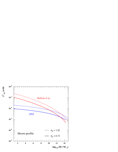
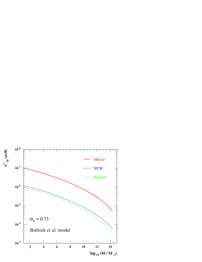
Figure 3: Average enhancement in the $\gamma$-ray flux emitted in a halo of mass $M$ at redshift $z=0$ with respect to the case in which the same amount of dark matter is smoothly distributed. On the left-hand side we show how sensitive the result is to the concentration parameter. On the right-hand side the result for three different families of dark matter density profiles is shown.

IV.1 Flux normalization

We analyze first how sensitive the flux is to the dark halo properties we discussed in Section III. In Fig. 3 – left panel – we plot $\Delta_{M}^{2}$ as a function of $M$, at redshift $z=0$ and assuming the Moore density profile to describe dark matter halos. The four cases displayed correspond to the two toy models for $c_{vir}$ we have discussed in the previous Section, and to two choices of $\sigma_{8}$: our default value $\sigma_{8}=0.73$ 2df and the larger value $\sigma_{8}=1.02$ found in another recent analysis pier and more on the line with values often quoted in the past. For small $M$, i.e. large $c_{vir}$, $\Delta_{M}^{2}$ scales roughly like $c_{vir}^{3}/\log^{2}(c_{vir})$, where the logarithmic term follows from the fact that the halo profiles we are considering have logarithmically divergent masses (which we cut at the virial radius). It follows that the uncertainty on $\sigma_{8}$ induces about a factor of 2 uncertainty on $\Delta_{M}^{2}$, while an indetermination of a factor of a few is due to the model applied to extrapolate $c_{vir}$ to small masses.

In Fig. 3 – right panel – we restrict to $c_{vir}$ as computed with the Bullock et al. toy model, and show the dependence of the signal on the choice of halo profile. The spread in the predictions between the Moore profile and the Burkert profile is around a factor of ten independent of mass, which is much smaller than the uncertainty due to the choice of profile when considering the dark matter induced $\gamma$-ray flux generated in single resolved sources. This is one of the advantages of considering the cosmological signal. Of course, one is also less sensitive to the actual halo properties of a single galaxy, the Milky Way, which are poorly known. This issue is analyzed further in Fig. 4 where, for a given halo of density profile $\rho(\vec{r})$, we plot the dimensionless quantity

$$\langle\,J\left(\psi\right)\rangle_{\Delta\Omega}=\frac{1}{\Delta\Omega}\frac{1}{8.5\,\rm{kpc}}\cdot\left(\frac{1}{0.3\,{\rm GeV}/{\rm cm}^{3}}\right)^{2}\int_{\Delta\Omega}d\,\Omega\int_{l.o.s.}d\,l\;\rho^{2}(\vec{r})\;,$$ (26)

a sum over contributions along the line of sight in a cone of aperture $\Delta\Omega$ in the direction $\psi$ (this quantity often appears in analyses of the WIMP induced flux generated in the Milky Way halo; normalization factors are fixed following the choice in Ref. bub ). We focus on a $10^{12}M_{\odot}{\ }$ halo, i.e. a halo of the size of the Milky Way or Andromeda, and assign to it the mean $c_{vir}$ in the Bullock et al model; also, we choose $\psi$ in the direction of the center of the halo and consider a moderately large acceptance angle, $\Delta\Omega=10^{-3}~{}\rm{sr}$. We let then the distance $d$ between the center of the halo and us vary between $10^{-3}R_{vir}$ and $10^{3}R_{vir}$ ($R_{vir}\sim 260\,\rm{kpc}$ in our sample case) and plot the corresponding $\langle\,J\,\rangle$ for the three halo profiles we introduced. The arrows in the figure marks the location on the horizontal axis of the Milky Way (MW) and Andromeda (M31). At large $d/R_{vir}$ we find for all halo profiles the $1/d^{2}$ scaling one expects for point-like sources: this is obvious for ratios larger than $d/R_{vir}\simeq\sqrt{\pi/\Delta\Omega}\simeq 56$, when the halo is fully contained in the field of view; however, as it can be seen, for the Burkert and the NFW profiles such scaling appears already for ratios one order of magnitude smaller, and it is present essentially over the whole range displayed for the Moore profile. This indicates that the bulk of the flux is emitted in the inner halos: for the Moore profile 50% (10%) of the total emitted flux is generated within a radius that is about $9\cdot 10^{-6}R_{vir}$ ($6\cdot 10^{-9}R_{vir}$), for the NFW and Burkert profiles the corresponding radii are shifted, respectively, to $2.4\cdot 10^{-2}R_{vir}$ ($3.3\cdot 10^{-3}R_{vir}$) and $6\cdot 10^{-2}R_{vir}$ ($2.4\cdot 10^{-2}R_{vir}$). While the spread in predictions for the flux generated in the center of our Galaxy is very large (6 orders of magnitude), the total emitted flux is a much weaker function of the density profile – the uncertainty is roughly an order of magnitude.

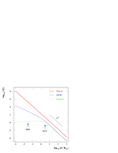
Figure 4: Scaling of the collected $\gamma$-ray flux with the distance $d$ between the detector and the center of a halo, for three different halo profiles. The angular acceptance of the detector is assumed to be $\Delta\Omega=10^{-3}\rm{sr}$. The plot is for a $10^{12}M_{\odot}{\ }$ halo, the arrows indicate the position on the horizontal axis for the Milky Way and Andromeda; the case for other masses is analogous.

This factor of 10 uncertainty is nearly independent of $M$, therefore it propagates as an order of magnitude uncertainty on the overall normalization of the WIMP induced $\gamma$-ray flux.

The behavior of $\Delta^{2}$ is obtained by folding the scaling of the integrated mass function in Fig. 1 with that of $\Delta_{M}^{2}$ in Fig. 3. The dominant contribution to $\Delta^{2}$ comes from very small halos: the integrand in $\Delta^{2}$ is the product of two mildly divergent quantities, the mass function times $M$ and $\Delta_{M}^{2}$; the result is still convergent but heavily relies on our understanding of the light mass end. This is shown in the left-hand panel of Fig. 5, where, for the Moore profile and our preferred cosmology, we plot $\Delta^{2}$ at $z=0$ restricting the range of integration over mass. For the Bullock et al. toy model the contribution per logarithmic interval keeps increasing even for the lightest mass range displayed, while in the ENS model it starts decreasing but rather slowly. Extrapolations of $c_{vir}$ with our toy models to exceedingly small masses may not be fully reliable; we prefer to introduce a cutoff in $c_{vir}$ and hence in $\Delta_{M}^{2}$ at the intermediate mass range $M_{cut}$, say $10^{5}M_{\odot}{\ }$ for $z=0$, where we believe the toy models are sufficiently trustworthy. We assume:

$$c_{vir}(M,z)=c_{vir}(M_{cut},z)\;\;\;\;\;\;\forall\;\;M<M_{cut}$$ (27)

The choice of $M_{cut}$ is to some extent arbitrary; should one make a different assumption Fig. 5 allows to scale our final results.

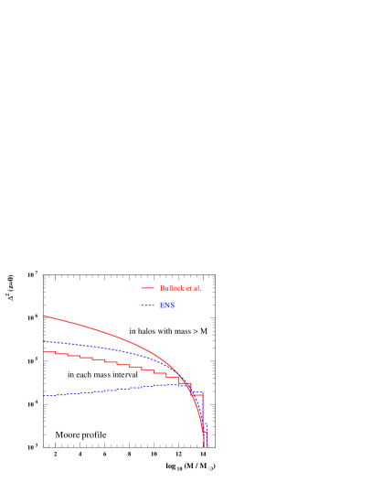
Figure 5: Enhancement in the diffuse $\gamma$-ray flux compared to the case when all structures in the Universe are erased. On the left-hand side the contributions of structures of given masses at $z=0$ are shown; on the right-hand panel we show the redshift dependence, rescaled with the term $(1+z)^{3}/h(z)$.

In Fig. 5 - right-hand panel, we plot $(1+z)^{3}\Delta^{2}/h$, i.e. the quantity we need to integrate over $z$ to get the $\gamma$-ray flux, see Eq. (23), once folded with the emission spectrum and the absorption factor. We consider both models for $c_{vir}$ and two schemes to define $M_{cut}$. In the first we fix $M_{cut}=10^{5}M_{\odot}{\ }$ for any $z$, progressively reducing the mass range over which $c_{vir}$ is extrapolated. Another possibility is to keep the range of this extrapolation fixed: at z=0 we choose $M_{\star}/M_{cut}$, with $M_{\star}$ the largest scale allowed defined implicitly by $\sigma\left(M_{\star}(z)\right)=\delta_{sc}(z)$ and again $M_{cut}=10^{5}M_{\odot}{\ }$; at other $z$ the same ratio is imposed (we never include extrapolations to masses lower than $10M_{\odot}{\ }$; at the redshift of a few when $M_{cut}$ would be lower than that, we set $M_{cut}=10M_{\odot}{\ }$). Both schemes are rather arbitrary, we will show however that the final result is not very sensitive to them. Notice, on the other hand, the sharp increase of $(1+z)^{3}\Delta^{2}$ at small $z$ for the ENS model, whereas a mild decrease or a flat behavior is found in the Bullock et al. model. At larger $z$, the scaling in $1/h(z)$ takes over.

IV.2 Spectral signatures

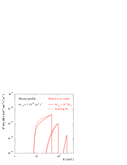
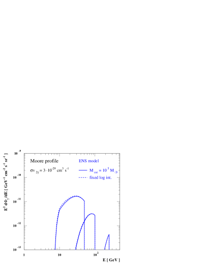
Figure 6: Spectral signature in the extragalactic gamma-ray flux due to the annihilation of dark matter WIMPs into monochromatic photons. A toy model with three choices of WIMP masses, $M_{\chi}=50,100,250$ GeV, and fixed annihilation rate into $2\gamma$, is considered. The signature arises because of the asymmetric distortion of the line due to the cosmological redshift, as well as, by absorption of gamma-rays generated in distant sources. The normalization of the fluxes are computed assuming halos are modelled by the Moore profile and concentration parameters are derived with the Bullock et al. toy model (left panel) or the ENS model (right panel); solid and dashed curves refers to two schemes for the choice of the halo mass cutoff $M_{cut}$, which, as can be seen, plays a marginal role.

We now try to estimate, in an approximate way, the level and spectral shape of the gamma-ray flux that can be expected for a general WIMP, leaving a more detailed discussion of the extragalactic background one has to fight against for Section V, and predicted signals for a more specific (supersymmetric) dark matter candidate for Section  VI.

The differential gamma-ray yield per WIMP pair annihilation can be written as:

$$\frac{dN_{\gamma}(E)}{dE}=\sum_{X}b_{\gamma X}n_{\gamma X}\delta\left(E-M_{\chi}\,(1-M_{X}^{2}/4\,M_{\chi}^{2})\right)+\sum_{F}b_{F}\frac{dN_{\rm cont}^{F}}{dE}(E)\;.$$ (28)

The first term refers to prompt annihilation into two-body final states containing a photon, which, forbidden at tree-level essentially by definition of dark matter (zero electric charge), are allowed at higher order in perturbation theory. Although subdominant, they have the peculiarity of giving monochromatic $\gamma$-rays: as WIMPs in halos are non-relativistic the energy of the outgoing photon is fixed by the WIMP mass $M_{\chi}$ and the mass of the particle $X$ (i.e., $E=M_{\chi}$ for the $2\gamma$ final state and $E=M_{\chi}(1-M_{X}^{2}/4\,M_{\chi}^{2})$ for final states with some non-zero mass particle $X$). The parameter $b_{\gamma X}$ is the branching ratio into these channels and $n_{\gamma X}$ is the number of photons per annihilation, i.e. 2 for the $2\gamma$ final state and to 1 for the others. The second term in Eq. (28) is instead the term due to WIMP annihilations into the full set of tree-level final states $F$, containing fermions, gauge or Higgs bosons, whose fragmentation/decay chain generates photons; this process gives rise to a continuous energy spectrum.

Although there is some span in the predictions for the photon emission rate in different particle physics models, the spectral features of the induced fluxes are quite generic and can be outlined without referring to a specific model (in section VI below we will discuss results for more specific models). We start discussing the monochromatic terms, focusing to be definite on the process $\chi\bar{\chi}\rightarrow 2\gamma$ and picking for reference some typical value for the annihilation cross section in this channel. Consider, e.g., that in the simplest case (no resonances or thresholds near the kinematically released energy in the annihilation $2M_{\chi}$) the WIMP total annihilation rate is fixed by the approximate relation jkg :

$$\sigma v\sim\langle\sigma v\rangle\sim\frac{3\cdot 10^{-27}\rm{cm}^{3}\rm{s}^{-1}}{\Omega_{\chi}h^{2}}\sim 3\cdot 10^{-26}\rm{cm}^{3}\rm{s}^{-1}\;,$$ (29)

which shows the order of magnitude scaling between the thermally averaged annihilation cross section $\langle\sigma v\rangle$ and the WIMP thermal relic abundance $\Omega_{\chi}$. Note that this relation is only a rough approximation and that large deviations from it can appear mainly due to resonances and thresholds. In Section VI below we will not use this approximate relation, but instead calculate the relic density including properly both coannihilations, resonances and thresholds. For the current discussion though, this approximate relation suffices. The annihilation into two photons is a 1-loop process so, in general, its strength is much smaller than $\sigma v$; we assume, as a sample case when this channel is relevant, $b_{2\gamma}=10^{-3}$.

In Fig. 6 we show the induced extragalactic gamma ray flux for 3 different values of the WIMP mass, $M_{\chi}=50,100,250$ GeV, and for the two schemes we have considered to estimate $c_{vir}$. We consider halos modeled by the Moore profile, with no subhalos (the effects of the latter will be discussed in Section IV.3). The figure illustrates the novel signature, first proposed in BEU, to identify a WIMP induced component in the measured extragalactic gamma-ray background, the sudden drop of the gamma-ray intensity at an energy corresponding to the WIMP mass due to the asymmetric distortion of the line caused by the cosmological redshift. The energy of the $\gamma$-rays at emission determines whether the smearing to lower energies has a sharper or smoother cutoff: for a larger $M_{\chi}$ the absorption on the extragalactic optical and infrared starlight background becomes more efficient. Spectra obtained applying the ENS toy-model for $c_{vir}$ are similar to those derived with the Bullock et al. model; the main difference, for masses lower than about 100 GeV, is a slight shift of the flux peak to lower energies. This effect, due to the sharp increase in $\Delta^{2}$ shown in Fig. 5 in a regime where the absorption factor does not rapidly take over, tends to reduce the difference in the flux normalization one might have foreseen looking at $\Delta^{2}_{M}$ alone (in the next generation of measurements the energy resolution will probably not be better than 10% or so). Fig. 6 also illustrates the fact that, at least for the line contributions, the treatment of the cutoff in halo mass is not very important; there is mainly an overall scaling with the choice of $M_{cut}$ at $z=0$, which the reader can infer from the left-hand panel of Fig. 5.

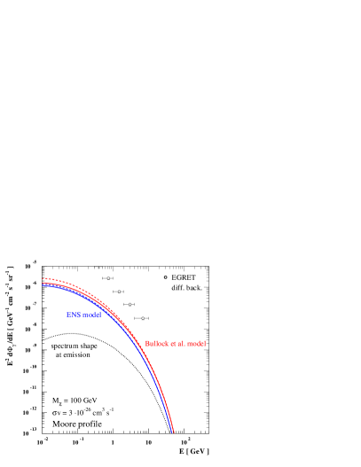
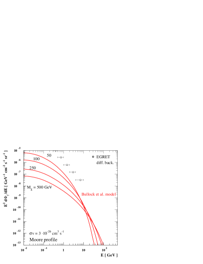
Figure 7: Spectral features for the extragalactic gamma-ray flux due to the photons with continuum energy spectrum emitted in pair annihilations of dark matter WIMPs. The cases considered here are for a WIMP toy model of given mass and fixed total annihilation rate, assuming the dominant branching ratio is $b\bar{b}$. The flux normalizations are computed under the same assumptions as in Fig. 6. In the left panel we compare the shape of the induced flux at Earth with the one at emission; in the right panel we show the dependence of the spectral shape on WIMP mass. For comparison, the EGRET estimate of the extragalactic background flux is shown.

Typical features in the continuum contribution are illustrated in Fig. 7. We have assumed again that $\sigma v\sim 3\cdot 10^{-26}\rm{cm}^{3}\,\rm{s}^{-1}$ and supposed that, as often happens in real particle physics models, the dominant annihilation channel is into $b\bar{b}$; the energy distribution per annihilating pair in their rest frame is simulated with the Pythia Monte Carlo package pythia . As most photons are produced in the hadronization and decay of $\pi^{0}$s (98.8% decay mode: $\pi^{0}\rightarrow 2\gamma$), the shape of the photon spectrum is peaked at half the mass of the pion, about 70 MeV, and is symmetric around it on a logarithmic scale (sometime this feature is called the “$\pi^{0}$ bump”, see, e.g., gaisser ). Had we chosen a different dominant annihilation channel or a combination of several channels, we would have found very similar behaviors. As absorption becomes negligible going to low energies, two features arise when summing extragalactic contributions over all redshifts: The peak in the spectrum is shifted to lower energies and there is a sharper decrease in the flux approaching the value of the WIMP mass. The first signature is probably hidden in background fluxes, see the discussion in the next Section. The second feature is instead potentially interesting, especially in case the line components are negligible: While a sensible contribution to the extragalactic $\gamma$-ray background can be provided by WIMPs in the few GeV energy range, at higher energies the WIMP induced flux is very rapidly suppressed. Such behavior cannot be associated to a spectral index, while background components are closer to a power law.

As shown on the right-hand side of Fig. 7, the WIMP-induced extragalactic flux gradually flattens for heavier and heavier WIMPs; also shown is the current estimate of the diffuse extragalactic background flux as derived from the analysis of data taken by the EGRET telescope Sreekumar98 .

IV.3 Role of subhalos

We have shown that small dense halos are providing the bulk of the WIMP induced $\gamma$-ray flux. So far we have considered just the case for isolated halos; as already mentioned, N-body simulations indicate that, in the clustering process with large halos forming by the merging of smaller objects, a fraction of the latter, up to about 10% of the total mass, may have survived tidal disruption and appear as bound subhalos inside virialized halos ghigna ; klypin99 . From the point of view of structure formation, the presence of rich substructure populations was at first seen as the main flaw in the picture from N-body simulations of $\Lambda$CDM cosmologies, a “crisis” urging for a solution ghigna ; klypin99 , maybe with a drastic change in the particle physics set up, see, e.g., da-ho . More recent analyses indicate that those results should be reinterpreted and the apparent discrepancy between the number of subhalos found in the simulations and that of luminous satellites observed in real galaxies is fading away, see, e.g., hayashi ; stoehr ; bullocketal ; bensonetal . From the point of view of dark matter detection, substructure may play a crucial role silkstebbins , even in the interpretation of currently available data. Consider, e.g., the gamma-ray halo surrounding the Galaxy for which statistical evidence has been claimed in data collected by the EGRET telescope dixon : the conjecture that this may be generated by pair annihilations of relic dark matter particles is based on the possible presence of dense dark matter clumps in the Milky Way halo grhalo .

At first sight, the role of substructure may seem marginal in our context. The fraction of mass in subhalos is small and the subhalo mass function is not likely to be significantly steeper than the mass function for isolated halos, Eq. (7). We expect then the number of halos in a given mass range to be larger than the number of substructures in the same range. On the other hand, the concentration parameter in subhalos may be significantly larger than for halos: on average, subhalos arise in higher density environments, as well as we expect a depletion in their outskirts by tidal stripping. This trend has indeed been observed in the numerical simulation of Ref. Bullock , where it is shown that, on average and for $M\sim 5\cdot 10^{11}M_{\odot}{\ }$ objects, the concentration parameter in subhalos is about a factor of 1.5 larger than for halos.

Consider a halo of mass $M$ and suppose that, on average, a fraction $f$ of its total mass is provided by substructures with mass function $dn_{s}/dM_{s}$. The differential energy spectrum for the number of photons emitted in such a halo, rather than by Eq. (21), is now given by:

$$\frac{d{\cal N}_{\gamma}}{dE}(E,M,z) = \frac{\sigma v}{2}\frac{dN_{\gamma}(E)}{dE}\left[\int dc^{\,\prime}_{vir}\;{\cal{P}}(c^{\,\prime}_{vir})\left(\frac{(1-f)\,\rho^{\prime}}{M_{\chi}}\right)^{2}\int d^{3}r\;g^{2}(r/a)\right.$$ (30)

$$\left.+\int dM_{s}\frac{dn_{s}}{dM_{s}}\int dc^{\,\prime}_{vir}\;{\cal{P}}_{s}(c^{\,\prime}_{vir})\left(\frac{\rho^{\prime}}{M_{\chi}}\right)^{2}\int d^{3}r\;g^{2}(r/a)\right]$$

$$= \frac{\sigma v}{2}\frac{dN_{\gamma}(E)}{dE}\frac{\bar{\rho}_{c}}{M_{\chi}^{2}}\left[(1-f)^{2}M\Delta_{M}^{2}(z,M)+\int dM_{s}\frac{dn_{s}}{dM_{s}}M_{s}\Delta_{M_{s}}^{2}(z,M_{s})\right]$$

A simple ansatz is that the subhalo mass function has a power-law behavior $dn_{s}/dM_{s}\propto 1/M_{s}^{\beta}$ for $M_{s}<M$ ($\beta<2\$ is required for the total mass to be finite), with the normalization fixed by using the definition of $f$, i.e.

$$\int dM_{s}M_{s}\frac{dn_{s}}{dM_{s}}=fM\;.$$ (31)

This gives

$$\frac{dn_{s}}{dM_{s}}=(2-\beta)f\frac{M^{\beta-1}}{M_{s}^{\beta}}\;.$$ (32)

If we further assume that $f$ and $dn_{s}/dM_{s}$ are independent of $M$, inserting Eq. (32) into Eq. (30), we find that the contribution of subhalos can be included in the formula for the gamma-ray flux, Eq. (23), with the replacement:

$$\Delta_{M}^{2}(z,M)\;\rightarrow\;(1-f)^{2}\;\Delta_{M}^{2}(z,M)+(2-\beta)fM^{\beta-2}\int dM_{s}\,M_{s}^{1-\beta}\,\Delta_{M_{s}}^{2}(z,M_{s})\;.$$ (33)

Here $\Delta_{M_{s}}^{2}$ is just $\Delta_{M}^{2}$ but with values of $c_{vir}$ and ${\cal{P}}(c^{\,\prime}_{vir})$ appropriate for the subhalos. It may be premature to deduce the latter from N-body simulation results. The scaling $c_{vir}\propto M^{-0.3}$ proposed in Ref. Bullock probably cannot be extrapolated to small masses: for $10^{5}M_{\odot}{\ }$ subhalos we would get a value of the concentration parameter 40 times larger than the value for halos as computed with the Bullock et al. toy model.

A prediction for the subhalo mass function is missing as well; there are just limited studies, not fully covering the mass range we are interested in. The current N-body simulation results are consistent with a power law behavior, but with non-universal slope and some indication that the index $\beta$ is getting harder decreasing the mass of the host halo. We find, e.g., from Fig. 5 in Ref. springel that $\beta\simeq 1.66$ for a $10^{15}M_{\odot}{\ }$ halo. A few studies are focused on Milky Way size halos, $10^{12}M_{\odot}{\ }$: from, e.g., Fig. 1 in Ref. stoehr we can extract the scaling $dn_{s}/dM_{s}\propto 1/M_{s}^{1.95}$.

The value of $f$ is a matter of debate as well. Values for the fraction of mass in substructures quoted in the literature are in the range 1 % to 10 % and they often refer to the ratio of the sum of the masses of identified subhalos to the total mass, rather than to an extrapolation performed assuming a mass function. Such a value, say $f^{\prime}$, should then depend both on the algorithm for finding subhalos in the simulation, and, most importantly, on the resolution of the simulation. Suppose that $f^{\prime}$ refers to a simulation where, for halos of mass $M$, substructures of mass down to $p\,M$ can be resolved; then, with our notation,

$$f^{\prime}M=fM^{\beta-1}\left[M^{2-\beta}-(p\,M)^{2-\beta}\right]\,,$$ (34)

i.e., $f=f^{\prime}/(1-p^{2-\beta})$. If $M=10^{12}M_{\odot}{\ }$ and $p=5\cdot 10^{-5}$ stoehr , we find $f=2.56f^{\prime}$. It is then not implausible that the true $f$, eventually to be found at future ultra-high resolution simulations, may approach or even exceed 10 %.

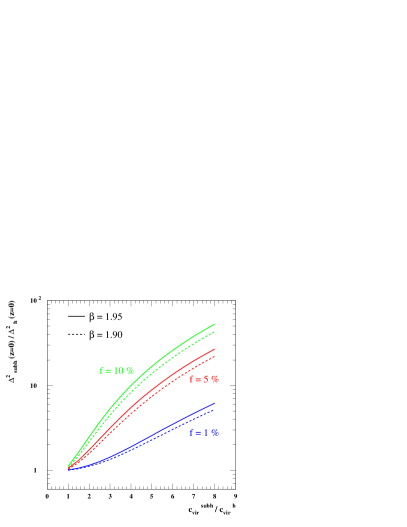
Figure 8: Influence of substructure on the flux normalization for three different average fractions $f$ of the total mass in subhalos; we have restricted to a specific mass function (see text) with spectral index $\beta$ and kept as a free parameter, we display on the horizontal axis the mean enhancement in the concentration parameter in subhalos.

To give a feeling for the possible effect of substructure, we consider the simplified sample case in which $f$ and the mass function are universal, and keep the average enhancement in the concentration parameter as a free parameter (we find the value of $c_{vir}(M,z)$ for subhalos by a rigid rescaling of the $c_{vir}(M,z)$ found for halos of same mass and at the same $z$: actually, the mass range in which this rescaling matters is just around the cutoff mass $M_{cut}=10^{5}M_{\odot}{\ }$). In Fig. 8 we consider $\beta=1.95$ or the slightly softer $\beta=1.90$, choose three sample values for the fraction of the mass in subhalos $f$ and plot the ratio of the value of $\Delta^{2}$ with and without including subhalos as a function of the average enhancement in the concentration parameter. Sensible gains in $\Delta^{2}$ and hence in the $\gamma$-ray flux normalization are viable even for moderate enhancements in the concentration parameter. Again, the effect of substructure is less dramatic than in case of single dark matter sources: the argument here is analogous to the one presented in the discussion on the role of the singularity in halo profiles.

IV.4 Observability of subhalos in the Milky Way halo

It would be of utmost importance to test the subhalo picture predicted by CDM N-body simulations by collecting information from the morphology of the Milky Way halo. As already mentioned, a rich population of luminous satellites is not observed in the Galaxy and this was considered, up to recent work, one the most severe “problems” of CDM. There are now models bullocketal ; bensonetal to explain why small substructures may be totally dark (without visible baryons); if this is indeed the case, WIMP annihilation might be the only chance to perform a detailed mapping of the distribution of mass in the Milky Way. This issue has been investigated by numerous authors (for a recent analysis see, e.g., Ref. clumps ). The problem however reduces to the study of the actual realization of incalculable random processes and this implies that it is very hard to estimate the probability for detection of a signal. In particular, a crucial parameter will be the location of the nearest dark matter clump, since this will dominate the signal. We show here how the picture we have outlined for a generic halo applies to the Milky Way and discuss the implications for the observability of subhalos.

The gamma-ray flux from a single “clump” of mass $M_{s}$ and at the distance $d$ from the Earth is equal to:

$$\frac{d\phi_{\gamma}^{1-cl}}{dE} = \frac{\sigma v}{2}\frac{dN_{\gamma}(E)}{dE}\frac{1}{4\pi}\int_{\Delta\Omega}d\,\Omega\int_{l.o.s.}d\,l\;\left(\frac{\rho(\vec{r})}{M_{\chi}}\right)^{2}$$ (35)

$$= 9.35\cdot 10^{-11}\left(\frac{\sigma v}{10^{-26}\;\rm{cm}^{3}\rm{s}^{-1}}\right)\left(\frac{100\;\rm{GeV}}{M_{\chi}}\right)^{2}\frac{dN_{\gamma}(E)}{dE}\Delta\Omega\;\langle\,J\left(\psi=0\right)\rangle_{\Delta\Omega}\;\rm{cm}^{-2}\rm{s}^{-1}\rm{GeV}^{-1}\,.$$

The angular extension of most clumps is much smaller than $\Delta\Omega$, hence we can use the point source approximation. In our formalism the formula becomes:

$$\frac{d\phi_{\gamma}^{1-cl}}{dE} = \frac{\sigma v}{2}\frac{dN_{\gamma}(E)}{dE}\frac{1}{4\pi\,d^{2}}\frac{M_{s}}{M_{\chi}^{2}}\,\frac{\Delta_{vir}\bar{\rho}_{0}}{3}\,\frac{(c^{\,\prime}_{vir}\,x_{-2})^{3}}{\left[I_{1}(c^{\,\prime}_{vir}\,x_{-2})\right]^{2}}\,I_{2}(x_{min},c^{\,\prime}_{vir}\,x_{-2})$$ (36)

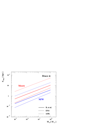
Figure 9: Maximum distance $d_{Max}$ of a clump from the our position in the Galaxy for which the $\gamma$-ray flux due to WIMP annihilations in the clump exceeds the estimated point source sensitivity of GLAST. We picked a specific WIMP dark matter candidate, while we are considering a few models to relate the mass of the clump $M_{s}$ to its concentration parameter, as well as two models for the halo density profiles in the clump (see the text for details)

Assume $\phi_{\gamma}(E>100\;\rm{MeV})>1.6\cdot 10^{-9}\rm{cm}^{-2}\rm{s}^{-1}$ Ritz-glast is the point source sensitivity of the next gamma-ray telescope in space, GLAST, which, as EGRET did, will map the whole gamma-ray sky. In defining a particle physics model for a WIMP, one has to fix $M_{\chi}$, $\sigma v$ and the branching ratios into each annihilation channel. It is then possible to compute, say,

$$N_{\gamma}^{100}=\int_{100\;\rm{MeV}}dE^{\prime}\frac{dN_{\gamma}(E^{\prime})}{dE^{\prime}}\,.$$ (37)

For each $M_{s}$ we can estimate the maximum distance $d_{Max}$ of the clump from us such that the WIMP induced flux is larger than the point source sensitivity of GLAST. This is shown in Fig. 9 for one of the WIMP toy models introduced in Ref. IV.2: we assume that $M_{\chi}=50\,\rm{GeV}$ and that the total annihilation rate into $b\bar{b}$ is $\sigma v=10^{-26}\;\rm{cm}^{3}\rm{s}^{-1}$, and find $N_{\gamma}^{100}=25.9$; a generalization to other models can be obtained very simply by scaling of these values. Six configurations for the normalization of the flux are chosen: we assume that $c_{vir}(M,z=0)$ for subhalos is either equal to the mean value found with the Bullock et al. or ENS toy models for isolated halos (labels “B. et al.” and “ENS” respectively) or to 4 times the value found with the Bullock et al. model (label “subh.”); we consider also the cases that subhalos are described both by the Moore et al. profile and by the NFW profile (the results for the Burkert profile are very close to the ones for NFW, unless the clump is very close to us, see Fig. 4). As can be seen, unfortunately, the prediction of our analysis is that just a few nearby clumps might be detected by GLAST. For comparison, we show the location in the plane of the figure of a “clump” that is sufficiently massive to have a luminous counterpart, Draco. This dwarf spheroidal, together with other similar candidates, has been considered several times in the literature as a potential gamma-ray dark matter source, see, e.g., tyler (note, however, that our picture applies on average, rather than to a single specific source, which might be better characterized through its rotation curve).

V The diffuse extragalactic gamma-ray background

The observability of the signal proposed here depends on the level of the diffuse extragalactic gamma ray background. Contributions from several classes of unresolved discrete sources have been discussed in the literature. After EGRET maps of the gamma-ray sky, the case for a dominant contribution from blazars is generally considered to be very strong: a large number of high-energy emitting blazars has been observed and, as we will show and contrary to other candidates, their distribution of energy spectra seems to be compatible with the observed extragalactic radiation. We will then rederive here the expected diffuse background under the assumption that the source of the background is unresolved blazars. We will mostly follow the analysis of Salamon and Stecker StSaMa93 ; SaSt94 ; StSa96 , but update it with more recent data and examine the expected uncertainties.

V.1 Basic blazar model

The basic model assumes that the diffuse gamma ray flux comes from unresolved blazars. We will assume that the blazars are distributed in redshift and luminosity according to a luminosity function $\rho_{\gamma}(P_{\gamma},z)$ where $P_{\gamma}$ is the luminosity (in units of W Hz^-1 sr^-1). The luminosity function $\rho_{\gamma}$ is the comoving density in units of Mpc^-3 (unit interval of $\log_{10}P_{\gamma/r}$)^-1. We will further assume that the blazars emit gamma rays with some spectral index $\alpha$ which is distributed according to a distribution function $p(\alpha)$. The absorption of gamma rays emitted at redshift $z$ and observed at energy $E_{0}$ is, as before, parameterized in terms of the optical depth $\tau(E_{0},z)$ such that the attenuation is proportional to $e^{-\tau(E_{0},z)}$. We will here use the parameterization of the Kennicut model in Primack et al. abs introduced in Section II. For comparison we will also use the model of Salamon and Stecker SaSt98 (their Fig. 6 with metallicity correction). There is also a recent estimate of the absorption by de Jager and Stecker deJaSt02 , but we will not use that model since it is not valid above $z\simeq 0.3$ which is not sufficient for our purpose. In EGRET observations one has seen that blazars most of the time are in a quiescent state but some small fraction of time are in a flaring state with higher luminosity and slightly different spectral index (softer, i.e. higher $\alpha$). We will assume that the blazars are in the flaring state a fraction $\zeta$ of their time and that their luminosity then is a factor $A_{f}$ higher than in the quiescent state. We will also parameterize the different spectral indices by assuming that they come from the same distribution function $p(\alpha)$ but shifted by $\Delta\alpha_{q}$ and $\Delta\alpha_{f}$ for the quiescent and flaring states respectively (these two quantities are not independent; we have adopted here the same notation as in Salamon and Stecker, but, alternatively, one could redefine $\alpha$ and introduce a single shift $\Delta\alpha$). Putting this together we can write the gamma ray flux (in units of cm^-2 s^-1 sr^-1 GeV^-1) at energy $E_{0}$ as

$$\phi_{\gamma}(E_{0}) = \frac{c}{H_{0}}\int_{\log_{10}P_{\gamma}^{\rm min}}^{\log_{10}P_{\gamma}^{\rm max}}d\log_{10}{P_{\gamma}}\int_{\alpha_{\rm min}}^{\alpha_{\rm max}}d\alpha\int_{z_{\rm min}}^{z_{\rm max}}dz$$ (38)

$$\frac{1}{h(z)}\frac{P_{\gamma}}{2\pi\hbar E_{\gamma,f}}\Big{[}p(\alpha-\Delta\alpha_{q})\rho_{\gamma,q}(P_{\gamma},z)+p(\alpha-\Delta\alpha_{f})\rho_{\gamma,f}(P_{\gamma},z)\Big{]}\frac{dN_{\gamma}}{dE}(E_{0}(1+z),\alpha)e^{-\tau(E_{0},z)}.$$

In this equation, we have introduced the following

$$\left\{\begin{array}[]{lcl}H_{0}&=&\mbox{Hubble constant today}\\ h(z)&=&\mbox{cosmology factor as defined in Eq.~{}(\ref{eq:hofz})}\\ E_{\gamma,f}=0.1~{}\mbox{GeV}&=&\mbox{the fiducial gamma ray energy at which the luminosity is $P_{\gamma}$}\\ \frac{dN_{\gamma}}{dE}&=&\mbox{the gamma ray spectrum (normalized to 1 at $E_{\gamma,f}$)}\\ \hbar&=&\mbox{Planck's reduced constant}\\ \rho_{\gamma,q}&=&\mbox{the luminosity function for blazars in quiescent state}\\ \rho_{\gamma,f}&=&\mbox{the luminosity function for blazars in flaring state}\end{array}\right.$$ (39)

Note that we have for clarity explicitly included $c$ and $\hbar$ in Eq. (38), but the unit conversion factors to get the flux in the above given units are not given explicitly. Note that there is no factor of $1/4\pi$ since the luminosity $P_{\gamma}$ is per sr already. We will, as before, assume that $H_{0}=70$ km s^-1 Mpc^-1, $\Omega_{m}=0.3$ and $\Omega_{\Lambda}=0.7$.

In the following subsections we will go through the different factors entering in Eq. (38).

V.2 The luminosity function $\rho_{\gamma}(P_{\gamma},z)$

We need to know the luminosity function as a function of redshift. Since not that many blazars are observed we will follow StSaMa93 ; SaSt94 ; StSa96 and assume that the same basic mechanism (i.e. the same population of high-energy electrons) is responsible for both the gamma ray and the radio flux. We can then use the much larger catalogs of radio sources to get the luminosity function. We will assume that the luminosities in gamma and radio are related by

$$\left\{\begin{array}[]{lcl}P_{\gamma,q}&=&\kappa P_{r}\\ P_{\gamma,f}&=&A_{f}\kappa P_{r}\end{array}\right.$$ (40)

where $P_{\gamma}$ and $P_{r}$ are the luminosities (in units of W Hz^-1 sr^-1). The gamma ray luminosity is given at 0.1 GeV and the radio luminosity at 2.7 GHz. The subscripts $q$ and $f$ refer to the quiescent and flaring states respectively. We will assume that the two luminosity functions are related by

$$\rho_{\gamma}(P_{\gamma},z)=\eta\rho_{r}(P_{r},z)$$ (41)

where $\rho_{\gamma}$ and $\rho_{r}$ are the luminosity functions (in units of Mpc^-3 (unit interval of $\log_{10}P_{\gamma/r}$)^-1). The factor $\eta$ takes into account possible beaming effects which could mean that not all radio blazars emit gamma rays towards the Earth (or vice versa). Including the effect that the blazars are assumed to be in the flaring state a fraction $\zeta$ of the time, we can finally write

$$\left\{\begin{array}[]{lcl}\rho_{\gamma,q}(P_{\gamma},z)&=&(1-\zeta)\eta\rho_{r}(\frac{P_{\gamma}}{\kappa},z)\\ \rho_{\gamma,f}(P_{\gamma},z)&=&\zeta\eta\rho_{r}(\frac{P_{\gamma}}{A_{f}\kappa},z)\end{array}\right.$$ (42)

For the radio luminosity function, we use the parameterization by Dunlop and Peacock DunlopPeacock90

$$\rho_{r}(P_{r},z)=10^{-8.15}\left[\left(\frac{P_{r}}{P_{c}(z)}\right)^{0.83}+\left(\frac{P_{r}}{P_{c}(z)}\right)^{1.96}\right]^{-1}\quad;\quad P_{c}(z)=10^{25.26+1.18z-0.28z^{2}}$$ (43)

valid up to $z=5$. This luminosity function was derived for a cosmology with $H_{0}=50$ km s^-1 Mpc^-1 and $\Omega_{0}=\Omega_{m}=1$, but we can approximately convert this to a luminosity function for our cosmology by multiplying $\rho$ with a correction factor DunlopPeacock90

$$\frac{dV_{\rm std}}{dV}=\frac{\left(\frac{(R_{0}S_{k}(r))^{2}}{H_{0}h(z)}\right)_{\Omega_{0}=\Omega_{m}=1,H_{0}=50~{}{\rm km\,s^{-1}\,Mpc^{-1}}}}{\left(\frac{(R_{0}S_{k}(r))^{2}}{H_{0}h(z)}\right)_{\rm our~{}cosmology}}$$ (44)

and multiplying $P_{c}(z)$ with the correction factor

$$\left[\frac{\left(D_{L}\right)_{\rm our~{}cosmology}}{\left(D_{L}\right)_{\Omega_{0}=\Omega_{m}=1,H_{0}=50~{}{\rm km\,s^{-1}\,Mpc^{-1}}}}\right]^{2}=\left[\frac{\left((1+z)R_{0}S_{k}(r)\right)_{\rm our~{}cosmology}}{\left((1+z)R_{0}S_{k}(r)\right)_{\Omega_{0}=\Omega_{m}=1,H_{0}=50~{}{\rm km\,s^{-1}\,Mpc^{-1}}}}\right]^{2}$$ (45)

where $D_{L}$ is the luminosity distance. The luminosity function Eq. (43) is valid between $P_{r}^{\rm min}=10^{18}$ W Hz^-1 sr^-1 and $P_{r}^{\rm max}=10^{30}$ W Hz^-1 sr^-1 which we will convert to limits on $P_{\gamma}$. Note that the exact upper and lower limits on the luminosity are unimportant since $P_{\gamma}\rho_{\gamma}$ that enters in Eq. (38) is peaked well between the lower and upper limits and is vanishingly small at the boundary. For the redshift integration we will as a default integrate between $z_{\rm min}=0$ and $z_{\rm max}=5$, but this integration range will be, as discussed below, restricted to include the effect of resolved blazars.

For the parameters $\kappa$, $\eta$, $\zeta$ and $A_{f}$, we will use the values obtained in StSa96 ,

$$\left\{\begin{array}[]{lcl}\kappa&=&4\cdot 10^{-11}\\ \eta&=&1.0\\ \zeta&=&0.03\\ A_{f}&=&5.0\\ \end{array}\right.$$ (46)

where $\kappa$ was determined from observations of blazars that are observed both in radio and in gamma rays, $\eta$ was determined by requiring the number counts of blazars to be consistent with the EGRET observations and $\zeta$ and $A_{f}$ was determined from EGRET blazar observations.

V.3 Intrinsic gamma ray spectrum

We will assume that the intrinsic gamma ray spectrum follows a power law with spectral index $\alpha$, i.e. that

$$\frac{dN_{\gamma}}{dE}=\left(\frac{E}{E_{f}}\right)^{-\alpha}$$ (47)

where $E_{f}=0.1$ is the fiducial energy at which we calculate the luminosity $P_{\gamma}$. Note that it is probably unrealistic to assume that the spectrum continues to be a power law to higher energies (above a few hundred GeV), instead we should expect a cut or a tilt in the spectrum. However, we will here for simplicity assume that there is no cut-off which means that we will probably overestimate the diffuse gamma ray background at high energies.

V.4 Flux from a single source

When taking resolved blazars into account we need the gamma ray flux a given blazar would produce. A blazar with luminosity $P_{\gamma}$ and spectral index $\alpha$ at redshift $z$ will give rise to the integrated gamma ray flux above energy $E_{th}$,

$$\Phi(E_{0}>E_{th})=\frac{P_{\gamma}}{2\pi\hbar E_{f}}\frac{E_{th}}{\alpha-1}\left(\frac{E_{th}(1+z)}{E_{f}}\right)^{-\alpha}\frac{1}{(R_{0}S_{k}(r))^{2}}.$$ (48)

This equation is valid for $E_{th}\lesssim 10$ GeV since we here have neglected absorption (which is a reasonable approximation for low energies). With appropriate unit conversions this is the flux in units of cm^-2 s^-1 that should be compared with the EGRET or GLAST point source sensitivity. For EGRET we will use the point source sensitivity $1\cdot 10^{-7}$ cm^-2 s^-1 egret-pss and for GLAST we will use $1.6\cdot 10^{-9}$ cm^-2 s^-1 Ritz-glast .

V.5 Distribution of spectral indices

We have to choose a distribution function for the spectral indices, $p(\alpha)$. One option is to use the distribution of spectral indices of blazars as observed by EGRET,

$$p(\alpha)=\frac{1}{N}\sum_{i}^{N}\frac{1}{\sigma_{i}\sqrt{2\pi}}e^{-\frac{(\alpha-\alpha_{i})^{2}}{2\sigma_{i}^{2}}}$$ (49)

where the sum is over the observed spectral indices $\alpha_{i}$ with their corresponding errors $\sigma_{i}$. However, this is not the best choice of distribution function since sources with low $\alpha$ are easier to detect due to their harder spectrum and we would hence introduce a selection bias. Instead we select a distribution function of the form

$$p(\alpha)=\frac{1}{\sigma_{\rm int}\sqrt{2\pi}}e^{-\frac{(\alpha-\alpha_{\rm int})^{2}}{2\sigma_{\rm int}^{2}}}$$ (50)

where we fix $\alpha_{\rm int}$ and $\sigma_{\rm int}$ such that the predicted distribution of $\alpha$ for observable blazars match the observed distribution. The predicted $\alpha$ distribution as it should be observed by EGRET is given by

$$p_{\rm obs}(\alpha)d\alpha = \frac{1}{N_{\rm pred}}\frac{4\pi c}{H_{0}}\int_{\log_{10}P_{\gamma}^{\rm min}}^{\log_{10}P_{\gamma}^{\rm max}}d\log_{10}{P_{\gamma}}\int_{z_{\rm min}}^{z_{\rm max}}dz$$ (51)

$$\frac{1}{h(z)}\Big{[}p_{\rm int}(\alpha-\Delta\alpha_{q})\rho_{\gamma,q}(P_{\gamma},z)+p_{\rm int}(\alpha-\Delta\alpha_{f})\rho_{\gamma,f}(P_{\gamma},z)\Big{]}\left(R_{0}S_{k}(r)\right)^{2}d\alpha.$$

where we only integrate over observable blazars, which is most easily done by noting that a blazar at redshift $z$, with luminosity $P_{\gamma}$ and spectral index $\alpha$ is observable if it would produce a flux above the EGRET point source sensitivity of $~{}1\cdot 10^{-7}$ cm^-2 s^-1 integrated above 0.1 GeV. Using Eq. (48) above we can for a given $P_{\gamma}$ and $\alpha$ calculate the maximum redshift $z^{\prime}$ at which such a blazar would be observable. This would then be our upper limit for the $z$-integration, i.e. $z_{\rm min}=0$ and $z_{\rm max}=z^{\prime}$. $N_{\rm pred}$ in Eq. (51) is the total number of observable blazars and is given by

$$N_{\rm pred} = \frac{4\pi c}{H_{0}}\int_{\log_{10}P_{\gamma}^{\rm min}}^{\log_{10}P_{\gamma}^{\rm max}}d\log_{10}{P_{\gamma}}\int_{\alpha_{\rm min}}^{\alpha_{\rm max}}d\alpha\int_{z_{\rm min}}^{z_{\rm max}}dz$$ (52)

$$\frac{1}{h(z)}\Big{[}p(\alpha-\Delta\alpha_{q})\rho_{\gamma,q}(P_{\gamma},z)+p(\alpha-\Delta\alpha_{f})\rho_{\gamma,f}(P_{\gamma},z)\Big{]}\left(R_{0}S_{k}(r)\right)^{2}$$

We now have to choose a sample of observed blazars and fit $\alpha_{\rm int}$ and $\sigma_{\rm int}$ such that we can reproduce the observed distribution of $\alpha$. We have followed this procedure for two samples of blazars, the first one are 27 blazars by Lin et al. Lin99 and the second one are the 65 blazars with determined spectral indices in the 3rd EGRET catalog Hartman99 . Before we do this fit, we fix the spectral shifts of blazars in quiescent and flaring states as

$$\left\{\begin{array}[]{lcl}\Delta\alpha_{q}&=&-0.05\\ \Delta\alpha_{f}&=&0.20\\ \end{array}\right.$$ (53)

which are the shifts determined by Stecker & Salamon StSa96 for EGRET blazars which have been observed in both quiescent and flaring states. For the two samples we then get

$$\left\{\begin{array}[]{lcl}\alpha_{\rm int}^{A}&=&2.25\\ \sigma_{\rm int}^{A}&=&0.30\\ \end{array}\right.\quad\mbox{Lin et al.\ \cite[cite]{\@@bibref{Authors Phrase1YearPhrase2}{Lin99}{\@@citephrase{(}}{\@@citephrase{)}}}}\qquad;\qquad\left\{\begin{array}[]{lcl}\alpha_{\rm int}^{B}&=&2.35\\ \sigma_{\rm int}^{B}&=&0.30\\ \end{array}\right.\quad\mbox{3rd EGRET catalog \cite[cite]{\@@bibref{Authors Phrase1YearPhrase2}{Hartman99}{\@@citephrase{(}}{\@@citephrase{)}}}}$$ (54)

These values are in very good agreement with the results in Sreekumar01 . We will refer to the first and second set of parameters as distribution A and B respectively. In Fig. 10a we compare distribution A with the predicted EGRET distribution and the observed EGRET distribution. In Fig. 10b we do the same thing for distribution B. Note that both predicted distributions fit the two observed samples rather well, but that the sample in the 3rd EGRET catalog is shifted by about 0.1 compared to the Lin et al. sample. This shift is of the same order as the expected systematic uncertainty in the EGRET catalog. In the following, we will use distribution A as our default since it reproduces the EGRET observed diffuse extragalactic background better than distribution B (see section V.6 below).

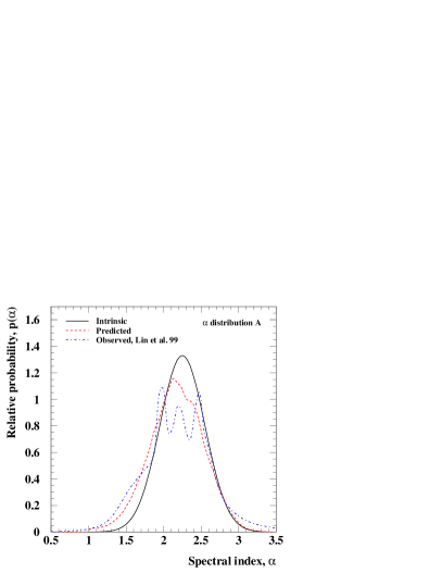
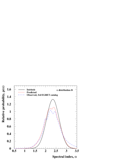
Figure 10: Different $\alpha$ distributions. a) The solid line is the intrinsic distribution A discussed in the text, the dashed is the predicted EGRET observable distribution and the dash-dotted line is the observed EGRET distribution for the Lin et al. sample Lin99 . b) The same as in a) but for intrinsic $\alpha$ distribution B and compared with the sample in the 3rd EGRET catalog Hartman99 .

The predicted number of observed blazars is given by Eq. (52) and for the two distributions we get $N_{\rm pred}^{A}=51$ and $N_{\rm pred}^{B}=42$, in reasonable agreement with the observed number of 66 blazars Hartman99 . Note that we do not expect perfect agreement since we only use a simple point source sensitivity, but in reality the sensitivity is much more complicated. We could easily envision that it should depend on e.g. the spectral index $\alpha$. Hence we are content that the agreement is as good as it is. Note that we also have the freedom to change the beaming parameter $\eta$, but we choose to keep it fixed to $\eta=1$ as given in Ref. StSa96 .

V.6 Taking resolved blazars into account

In Eq. (38) we should only integrate over unresolved blazars. This is done in the same way as in the previous section, i.e. for a given luminosity $P_{\gamma}$ and spectral index $\alpha$ there is a given redshift $z^{\prime}$ below which the blazars will be resolved and above which they will be unresolved. If we let the lower limit of the redshift integration, $z_{\rm min}$ be equal to this redshift $z^{\prime}$ we will only include unresolved blazars.

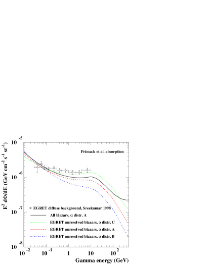
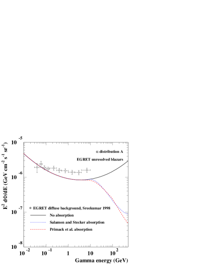
Figure 11: The predicted diffuse gamma ray flux (multiplied by $E^{2}$ to show features more clearly) for EGRET. a) The predicted fluxes for different $\alpha$ distributions. Distribution C is like A and B but with $\alpha_{\rm int}=2.15$. As can be seen the exact shape of the spectrum is fairly sensitive to the $\alpha$ distribution. Also shown are the EGRET measurements of the diffuse extragalactic gamma ray background. b) The predicted flux for different absorption models.

In Fig. 11 we show the predicted diffuse gamma ray fluxes for EGRET. As can be seen in a), our model reproduces the measured diffuse extragalactic background Sreekumar98 fairly well. To further illustrate the dependence on the $\alpha$ distribution, we also show results for a hypothetical $\alpha$ distribution (C) with $\alpha_{\rm int}=2.15$. For this distribution, the agreement with the EGRET measurements is excellent (the slight difference in normalization could be fixed by slightly increasing the beaming parameter $\eta$). We should note that our predictions are fairly sensitive to the exact low-$\alpha$ behavior of $p(\alpha)$. The higher up in energy we go, the more we sample the low-$\alpha$ region. In b) we show the effects of the different absorption models. It is clear that as soon as we go above 10–100 GeV, absorption effects are very important. Also keep in mind that we have not included a cut-off in the intrinsic gamma ray spectrum which would further reduce the fluxes at high energy.

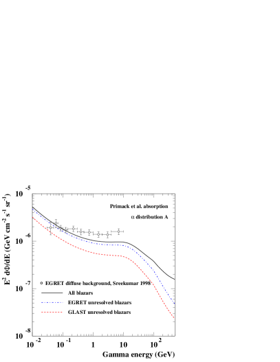
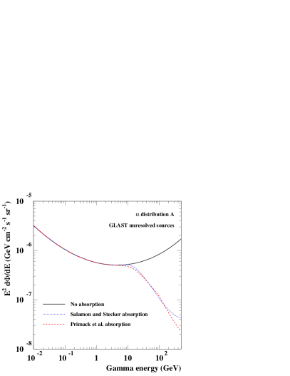
Figure 12: The predicted diffuse gamma ray flux (multiplied by $E^{2}$ to show features more clearly) for GLAST. a) The predicted fluxes compared to the EGRET measurements. b) The predicted fluxes for different absorption models.

In Fig. 12a we show the effect of different point source sensitivities. We see that compared to EGRET, the superior point source sensitivity of GLAST will reduce the diffuse gamma ray background with roughly a factor of two. Note however, that the angular resolution of GLAST will make the point source sensitivity worse at lower energies (or rather, larger spectral indices $\alpha$), an effect we have not included here. We expect that this effect would make the predicted background for GLAST slightly higher at low energies than shown in the figure. In Fig. 12b we show the effect of different absorption models for the predicted GLAST gamma ray background.

V.7 Uncertainties

In this section we have produced a derivation of the expected diffuse gamma ray background assuming that it is due to unresolved blazars. There are many uncertainties involved. First of all, it is not known whether blazars are the only sources relevant to compute the background. The energy spectrum of the blazars is also not very well known, i.e. there could be a cut-off at high energies (and even if the spectrum is a power law, the distribution of spectral indices is uncertain). Even the luminosity function is rather uncertain and the assumption of the relation between the gamma and radio luminosity functions cannot be tested until the sample of blazars measured in both gamma and radio increases. The parameters of the model we discussed are also quite uncertain, and, as already mentioned, gamma ray absorption introduces further uncertainties, especially at high energies. In spite of all these uncertainties, the agreement we find between our prediction and EGRET data is quite good, and gives some credibility to our estimate of the background for GLAST at higher energies. We have chosen as our default model the $\alpha$ distribution A, which reproduces both the measured $\alpha$ distribution and the EGRET energy spectrum satisfactory, and the absorption model of Primack et al. Keep in mind though that, above $\sim 100$ GeV, the uncertainties can be as large as a factor of a few.

VI Applications to supersymmetric dark matter

VI.1 A few examples in a specific particle physics setup

So far, we have kept the discussion as general as possible, without specifying the exact identity of the WIMP making up the dark matter. To gauge the possibility of detecting a gamma-ray signal in a realistic scenario, we now investigate one of the prime candidates for dark matter: the lightest supersymmetric particle (LSP) in the MSSM - the minimal supersymmetric extension of the Standard Model of particle physics. If R-parity is conserved, the LSP is stable; furthermore, its coupling with lighter standard model particles ensures that a population of such particles is present in the early Universe, with its density set by thermal equilibrium. The freeze out from equilibrium is roughly set by the LSP thermally averaged annihilation cross section; as sketched in Eq. (29), a weak interaction strength coupling ensures that WIMPs have a thermal relic abundance of the order of the critical density: this is naturally the case if the LSP has zero electric and color charges.

We thus take as our template WIMP dark matter candidate the lightest neutralino, $\tilde{\chi}^{0}_{1}$, in the MSSM (see lbreview for a recent review). $\tilde{\chi}^{0}_{1}$ is defined as the lightest mass eigenstate obtained from the superposition of four spin-1/2 fields, the Bino and Wino gauge fields, $\tilde{B}$ and $\tilde{W}^{3}$, and two neutral CP-even Higgsinos, $\tilde{H}^{0}_{1}$ and $\tilde{H}^{0}_{2}$:

$$\tilde{\chi}^{0}_{1}=N_{11}\tilde{B}+N_{12}\tilde{W}^{3}+N_{13}\tilde{H}^{0}_{1}+N_{14}\tilde{H}^{0}_{2}\;.$$ (55)

There are large regions in the MSSM parameter space where Bino-like LSPs or neutralinos with relevant Higgsino components have a thermal relic abundance of the right order to account for the dark matter, see, e.g., coann . We have used the DarkSUSY package ds to scan extensively the parameter space and generate a large archive of such models. We select those models that do not violate present accelerator and astrophysical limits and study what is the typical gamma-ray yield, both for the continuum and monochromatic spectra (in the MSSM there are two line signals allowed: $\gamma\gamma$ and $Z\gamma$). With DarkSUSY ds we calculate the relic density by numerically solving the Boltzmann equation properly taking resonances, thresholds and coannihilations (between the lightest neutralinos and other neutralinos and charginos) into account coann .

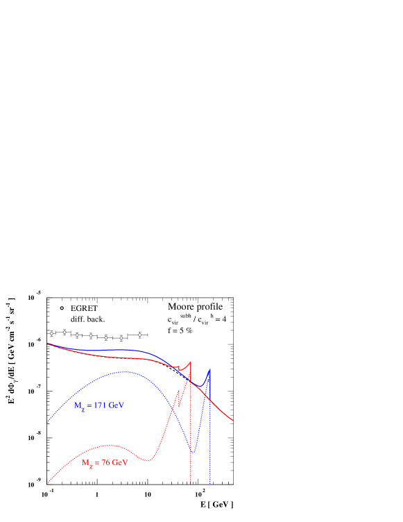
Figure 13: Extragalactic gamma-ray flux (multiplied by $E^{2}$) for two sample thermal relic neutralinos in the MSSM (dotted curves), summed to the blazar background expected for GLAST (dashed curve). Normalizations for the signals are computed assuming halos are modelled by the Moore profile, with 5% of their mass in substructures with concentration parameters 4 times larger than $c_{vir}$ as estimated with the Bullock et al. toy model.

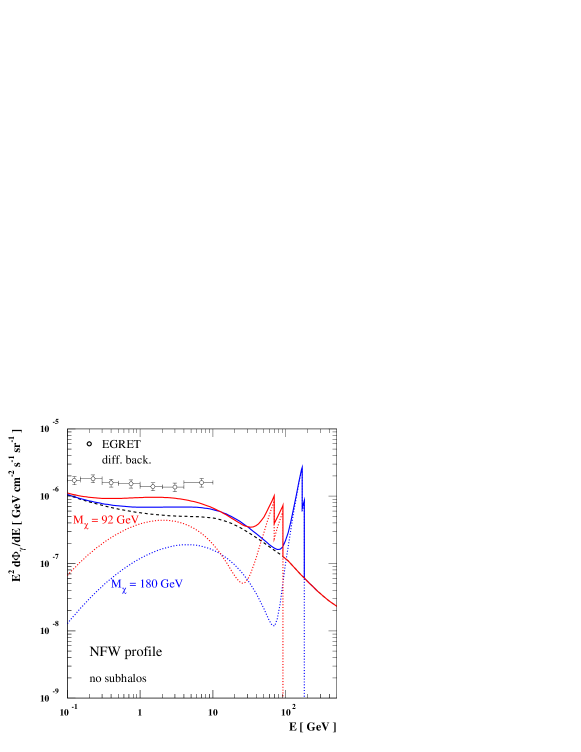
Figure 14: Extragalactic gamma-ray flux (multiplied by $E^{2}$) for two sample non-thermal dark matter candidates arising in the AMBS scenario (dotted lines) compared to the expected background (dashed curve). Annihilations cross sections are in these cases larger than for the models displayed in Fig. 13, however a different normalization for the fluxes is implemented here: we consider the case for halos modelled by the NFW profile, no substructures and concentration parameters inferred from the Bullock et al. toy model.

We focus first on neutralinos with a relic abundance $\Omega_{\chi}h^{2}$ in the interval 0.1 to 0.2, corresponding to our preferred cosmology $\Omega_{M}\sim 0.3$ and $h\sim 0.7$. There are models with $\sigma v_{2\gamma}\gtrsim 10^{-29}\rm{cm}^{3}\rm{s}^{-1}$ over the whole mass range from 50 GeV up to a few TeV. We consider two sample cases and plot the corresponding extragalactic $\gamma$-ray spectra in Fig. 13 (dotted lines). The first model has $M_{\chi}$ = 76 GeV, relatively low total annihilation cross section $\sigma v=6.1\cdot 10^{-28}\rm{cm}^{3}\rm{s}^{-1}$ but large branching ratios into photon states, $b_{2\gamma}=6.1\cdot 10^{-2}$ and $b_{Z\gamma}=5.2\cdot 10^{-2}$. The other has $M_{\chi}$ = 171 GeV, larger annihilation rate $\sigma v=4.5\cdot 10^{-26}\rm{cm}^{3}\rm{s}^{-1}$ but $b_{2\gamma}=5.2\cdot 10^{-4}$ and negligible branching ratio into the $Z\gamma$ final state. The normalization of the flux is set by assuming that dark matter structures are described by the Moore profile, with concentration parameters as computed with the Bullock toy model, and assuming the presence of a moderate amount of substructure, $f=5\%$, with a factor of 4 enhancement in $c_{vir}$. Under these assumptions, the neutralino induced $\gamma$-ray flux is at the level of the diffuse background from unresolved blazars ($\alpha$ distribution A) expected in GLAST, with the peak from the monochromatic emission significantly above it (dashed curves refer to the background only, solid curves to the sum of signal plus background).

The condition $\Omega_{\chi}h^{2}>0.1$ sets an upper bound on to the total annihilation cross section and hence, indirectly, an upper bound on the strength of the monochromatic channels; such states however are not the dominant modes and therefore a lower bound does not follow from imposing $\Omega_{\chi}h^{2}<0.2$: there are cases where the $\tilde{\chi}^{0}_{1}$ is compatible with being a good dark matter candidate, but the monochromatic flux is negligible. An opposite conclusion holds for the continuum components: there are cases in which the gamma-ray yield can be slightly larger than the one for the $M_{\chi}$ = 171 GeV model, but very small regions in parameter space where the yield is significantly smaller than for the model with $M_{\chi}$ = 76 GeV we show.

If we remove the constraint on $\Omega_{\chi}$ the picture can change drastically. In particular, there are several schemes in which the LSP relic abundance today is not set by its thermal relic density. One example is the case for Wino or Higgsino-like neutralinos in the version of the MSSM with anomaly mediation for supersymmetry breaking (AMSB). This scheme induces a mapping into regions in the MSSM parameter space in which the thermal relic abundance is negligible; however, an additional “non-thermal” relic source is present due to decays into neutralinos of gravitinos or moduli fields, fields that parameterize a flat direction of the theory and that dominate the energy density in the early Universe ggw ; mr . One can show that, in this context, the total annihilation rate, as well as cross sections in the $2\gamma$ and $Z\gamma$ final states, are forced to be very large anom . Two examples are shown in Fig. 14: one model has $M_{\chi}$ = 92 GeV, $\sigma v=2.5\cdot 10^{-24}\rm{cm}^{3}\rm{s}^{-1}$, $b_{2\gamma}=1.2\cdot 10^{-3}$ and $b_{Z\gamma}=2.2\cdot 10^{-3}$; the second $M_{\chi}$ = 180 GeV, $\sigma v=2.2\cdot 10^{-24}\rm{cm}^{3}\rm{s}^{-1}$, $b_{2\gamma}=1.8\cdot 10^{-3}$ and $b_{Z\gamma}=5.1\cdot 10^{-3}$. The normalization of the two extragalactic $\gamma$-ray fluxes is set assuming NFW halo profiles with no substructure and concentration parameters as computed with the Bullock toy model. Had we chosen the Moore profile rather than NFW, the predicted fluxes would be one order of magnitude larger, hardly compatible with the extragalactic flux as inferred from EGRET data. Note that a flux at roughly the same level is expected implementing the Burkert profile, hence the detectability of this signal is not linked to having a singular halo profile describing dark matter halos.

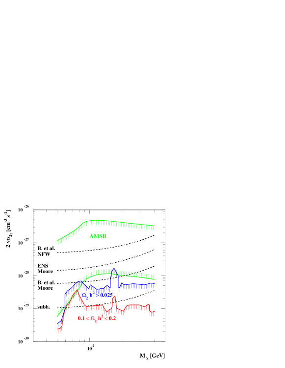
Figure 15: Approximate $3\sigma$ sensitivity curves for the GLAST telescope to search for a component in the extragalactic gamma-ray flux induced by WIMP annihilations into monochromatic photons. The sensitivity curves are plotted in the plane WIMP mass (coinciding with the energy peak in the induced flux) versus twice the annihilation rate into two photons, and for four configurations to estimate the normalization of the flux (the highest and lowest dashed curves correspond, respectively, to the choice in Fig. 14 and Fig. 13). Also shown is the range of the predictions of $v\sigma_{2\gamma}$ for neutralinos in the AMSB scenario, and the upper limit to it in case of thermal relic neutralinos in the MSSM, assuming their relic abundance is either in the cosmologically preferred mass range $0.1<\Omega_{\chi}h^{2}<0.2$, or in the less restrictive range often considered $0.025<\Omega_{\chi}h^{2}<0.2$.

VI.2 Sensitivity in upcoming measurements

It is not straightforward to estimate the smallest WIMP induced component GLAST will be able to disentangle from the background. A firm statement about the possibility to single out the yield with continuum energy spectrum will be possible only when higher precision measurements will allow to characterize better the level and the spectral features of the background. The monochromatic component has a much better signature and might be unambiguously identified. We make an attempt to make a rough estimate of the sensitivity curves for a GLAST-like instrument under a few schematic assumptions.

We assume the instrument has a peak effective area of 8000 cm² at energies above 10 GeV and an average energy resolution of 15% Ritz-glast . We take an exposure of 4 years, mapping the whole sky except for the regions already excluded in the EGRET analysis Sreekumar98 , i.e. the galactic plane $|b|<10^{\circ}$, and the bulge $|l|<40^{\circ}$ and $|b|<30^{\circ}$, with an average effective area which is about $20\%$ of the peak area. We set up a $\chi^{2}$ procedure to check if we can discriminate the spectrum of a line signal superimposed on the background from the spectrum of the background only. The analysis is performed assuming a given normalization for the WIMP flux and keeping as free parameters the value of the WIMP mass and annihilation cross section $\sigma v_{2\gamma}$. For each parameter choice, we sum to this flux the diffuse background from unresolved blazars ($\alpha$ distribution A) with the normalization computed in the previous Section and already shown in Figs. 13–14. We then perform a binning of the spectrum above 10 GeV, optimizing the bin width as a function of the number of events in each bin and checking that we have at least 10 events per bin. Naively, the statistical error in each bin would be the square root of the number of events in the bin; at second thought though, the extragalactic background component will be obtained after subtracting point sources and the diffuse galactic emission, with a non trivial propagation of errors we cannot easily retrace here. We make a simplifying assumption at this stage, expecting just a rough estimate of the true sensitivity curves. Suppose the main component one has to fight against is due to diffuse galactic $\gamma$-rays; such a component can be removed after assuming a model for diffuse emission and should be, on average, about an order of magnitude larger than the extragalactic component Sreekumar98 . We mimic this subtraction by assuming that the error in each energy bin is the square root of the number of events in the bin multiplied by 10. We then use the $\chi^{2}$ criterion to discriminate whether or not the obtained distribution of events can be fitted at 3 $\sigma$ with a background component only with fixed spectral shape but arbitrary normalization.

The corresponding sensitivity curves are shown in Fig. 15 in the plane neutralino mass - twice the $2\gamma$ annihilation rate. Each curve corresponds to a different normalization for the extragalactic flux: from the bottom up, case for Moore profile halos with substructure introduced already in Fig. 13, the case for Moore profile halos with no substructure and concentration parameters as computed with the Bullock et al. toy-model or with the ENS model, and, finally, the case for NFW halos with no substructure and $c_{vir}$ as in the Bullock et al. model. Also shown in the picture are the span in the predictions for $\sigma v_{2\gamma}$ in the AMSB scenario anom (green lines marks the upper and lower limits for a given mass), and approximate upper limits in the case of MSSM thermal relic neutralinos with relic abundance in the preferred range $0.1<\Omega_{\chi}h^{2}<0.2$, or in the less restrictive range often considered $0.025<\Omega_{\chi}h^{2}<0.2$, as deduced from our sampling of the parameter space. As can be seen, depending on the configuration one considers, there is a fair chance that the monochromatic $\gamma$-ray flux will be disentangled from GLAST data. The four models we have considered in Figs. 13 and 14 lie all above the corresponding sensitivity curves.

The same sensitivity curve can be applied to the case of the line signals generated in the $Z\gamma$ channel by replacing $M_{\chi}$ on the horizontal axis with the energy of the peak $E=M_{\chi}(1-M_{Z}^{2}/4\,M_{\chi}^{2})$ and assuming the quantity on the vertical axis is $\sigma v_{Z\gamma}\cdot 4E^{2}/(E+\sqrt{E^{2}+M_{Z}^{2}})^{2}$.

VI.3 Comparison with other signals

It is not straightforward to compare the dark matter signal we have presented here with other indirect signals which were proposed soon after the idea of WIMP dark matter was raised, two decades ago. Most analyses have been devoted to the study of the detectability of gamma-rays produced in the halo of our own Galaxy or of antimatter generated by WIMP pair annihilations taking place in our local environment (say within a few kpc, the exact number depends on the model for propagation of charged cosmic rays), refining the original proposals, see lbreview for a detailed reference list.

As already mentioned, the prospects for detecting gamma-rays produced in the Milky Way are much more tightened to assumptions on the distribution of dark matter WIMPs in the galactic halo. The monochromatic flux generated by the sample MSSM models displayed in Fig. 13 and Fig. 14 in the Galactic center region is within the sensitivity of GLAST or the upcoming generation of ground based air Cherenkov telescopes (see, e.g., the analysis in Ref. anom ) if indeed the dark matter density profile is singular, respectively, as in the Moore et al. or the NFW halo all the way to the central black hole (or maybe even steeper than that, see the possible enhancement induced by the black hole formation discussed in GS , but take into account also the opposite conclusions drawn in, e.g., Refs. spike ; milo ). As suggested also by Fig. 4, even a slight depletion in the central density can change drastically this conclusion.

We checked also that the four sample MSSM models we introduced, with the halo profiles considered in the corresponding figures, do not generate a continuum spectrum component which exceeds the flux measured by the EGRET telescope MH . A comparison with the Galactic flux at high latitudes in a configuration with clumps in the halo is much more uncertain. The flux is dominated by eventual nearby clumps, depending critically on the actual physical realization which happens to correspond to the Milky Way: we recall, on the other hand, that the signal we propose is obtained as the sum of many unresolved sources, i.e. we are automatically making an average over a set of possible configurations. The chance for GLAST to resolve single clumps, for the sample configurations with clumps considered in Fig. 13, can be read out of Fig. 9. The models with neutralino masses $M_{\chi}=$ 76, 171 GeV, have, respectively, $N_{\gamma}^{100}=$ 27.4 and 39.9; hence dotted lines corresponding to the Moore profile in Fig. 9 should be rescaled along the vertical axis by, respectively, a factor of 0.096 and 0.45.

Limits from charged cosmic ray data are also model dependent, as again the dark matter signal is dominated by local sources; dark matter candidates may be excluded in some configurations, but allowed in others. Notice also that, especially if one focusses on the monochromatic gamma-ray component, such a signal is very weakly correlated to the production rate of e.g. antiprotons and positrons, see, e.g., clumpy .

VII Conclusions

We have studied predictions and the observability of the diffuse gamma ray signal from WIMP pair annihilations in external halos. We have found configurations that imply signals at a detectable level for GLAST, the upcoming gamma-ray space telescope, both for non-thermal dark matter neutralinos, such as in the anomaly-mediated supersymmetry breaking model, and for thermal relic neutralinos in the MSSM. The key ingredient to show that detectable fluxes may arise, which was neglected in early estimates, is the picture, inspired by the current theory for structure formation and by N-body simulation results, that dark matter clusters hierarchically in larger and larger halos, with light structures more concentrated than more massive ones. For dark matter candidates in the AMSB scenario our conclusion holds independently of further assumptions on the dark matter distribution inside halos. Pair annihilation cross sections for thermal relic WIMPs are generally smaller; this however can be compensated by the enhancement in the flux one finds if, as suggested by results of simulations, we assume that dark matter profiles are singular and contain small dense substructures.

If the branching ratio for WIMP annihilation into monochromatic gamma rays is significant (about a few times $10^{-4}$ or larger), the induced extragalactic flux shows a very distinctive feature, the asymmetric distortion of the line due to the cosmological redshift and its sudden drop at the value of the WIMP mass. The component with continuum energy spectrum can be at the level of background components but has less distinctive features: the flux is characterized by the “$\pi^{0}$ bump”, rather than by a spectral index, with the peak shifted to energies lower than $M_{\pi}/2$ and the width set by the WIMP mass. Once a better measurement of the background will be available, it will be possible to address the question of whether or not this signal can be disentangled from other eventual components.

We have discussed in detail how our predictions depend on assumptions on the Cosmological model and the structure formation picture applied. Unless one introduces drastic changes, such as a large warm dark matter component, the cosmological parameters in the CDM setup do not play a major role; results are mainly sensitive to $\sigma_{8}$ with about a factor of two uncertainty. Larger indeterminations, of the order of a factor of a few, are introduced when estimating the scaling of the concentration parameter with halo mass, as extrapolations with toy models out of the mass range of N-body simulation results are needed. The functional form of the dark matter profile in single halos introduces a factor of 10 uncertainty, going from the case of a $1/r^{1.5}$ cusp in the Moore profile to the case of non-singular profiles; that uncertainty is much smaller than, e.g., the one induced on the estimate of the flux from the center of our own Galaxy. The presence of substructures inside halos may provide a factor of a few enhancement in the flux, but this effect is more difficult to address: we have presented a simple and rather generic setup, which will be possible to refine when further information on halos will be provided by higher resolution numerical simulations.

Issues related to the estimate of the background are very important as well. We have presented here a novel estimate of the expected background from unresolved blazars in GLAST, exploiting recent data and discussing critically the uncertainties involved, including the role played by gamma absorption.

Concluding, the present analysis has been devoted to examining in detail an idea that three of the authors have recently presented in a short letter beu . This work provides further support for such proposal, with exciting perspectives for upcoming measurements.

P.U. was supported by the RTN project under grant HPRN-CT-2000-00152. J.E. and L.B. wish to thank the Swedish Research Council for support.

References

- (1) L. Bergström, Rept. Prog. Phys. 63, 793 (2000) [arXiv:hep-ph/0002126].
- (2) C. B. Netterfield et al. [Boomerang Collaboration], arXiv:astro-ph/0104460; N. W. Halverson et al. [DASI Collaboration], arXiv:astro-ph/0104489; R. Stompor et al. [MAXIMA Collaboration], Astrophys. J. 561, L7 (2001) [arXiv:astro-ph/0105062].
- (3) S. Perlmutter et al., Astrophys. J. 517, 565 (1999); A. Riess et al., Astron. J. 116, 1009 (1998).
- (4) L. Verde et al. (2dF Collaboration), arXiv:astro-ph/0112161.
- (5) W.J. Percival et al., [arXiv:astro-ph/0206256].
- (6) B. Moore, plenary talk at 20th Texas Symposium, arXiv:astro-ph/0103100.
- (7) J. Primack, arXiv:astro-ph/0112255.
- (8) L. Bergström, J. Edsjö and P. Ullio, Phys. Rev. Lett. 87, 251301 (2001) (BEU).
- (9) J.E. Gunn, B.W. Lee, I. Lerche, D.N. Schramm and G. Steigman, Astrophys. J. 223, 1015 (1978); F.W. Stecker, Astrophys. J. 233, 1015 (1978); J.S. Silk and M. Srednicki, Phys. Rev. Lett. 53, 624 (1984); Y.-T. Gao, F.W. Stecker and D.B. Cline, Astronomy and Astrophys. 249, 1 (1991).
- (10) G. Kauffmann, S.D.M. White and B. Guiderdoni, Astrophys. J. 264, 201 (1993).
- (11) S. Cole et al., MNRAS 271, 781 (1994).
- (12) J.E.G. Devriendt and B. Guiderdoni, Astron. Astrophys. 363, 851 (2000).
- (13) M.H. Salamon and F.W. Stecker, Astrophys. J. 493, 547 (1998).
- (14) O.C. de Jager and F.W. Stecker, Astrophys. J. 566, 738 (2002).
- (15) J.R. Primack, R.S. Somerville, J.S. Bullock and J.E.G. Devriendt, eprint astro-ph/0011475 (2000).
- (16) W. Press and P. Schechter, Astrophys. J. 187, 425 (1974).
- (17) V.R. Eke, S. Cole and C.S. Frenk, MNRAS 282, 263 (1996).
- (18) P.J.E. Peebles, “Principles of physical cosmology”, Princeton University Press, 1993.
- (19) J.M. Bardeen, J.R. Bond, N. Kaiser and A.S. Szalay, Astrophys. J. 304, 15 (1986).
- (20) J.A. Peacock, “Cosmological physics”, Cambridge University Press, 1999.
- (21) W. Hu and N. Sugiyama, Astrophys. J. 471, 542 (1996).
- (22) R.K. Sheth, H.J. Mo and G. Tormen, MNRAS 323, 1 (2001).
- (23) A. Jenkins et al. (The Virgo Consortium), Astrophys. J. 499, 20 (1998).
- (24) O. Lahav et al. (The 2dF Team), astro-ph/0112162.
- (25) J.F. Navarro, C.S. Frenk and S.D.M. White, Astrophys. J. 462, 563 (1996); Astrophys. J. 490, 493 (1997).
- (26) C. Power et al., astro-ph/0201544.
- (27) B. Moore, T. Quinn, F. Governato, J. Stadel and G. Lake, MNRAS 310, 1147 (1999).
- (28) A. Klypin, A.V. Kravtsov, J.S. Bullock and J.R. Primack, Astrophys. J. 554, 903 (2001).
- (29) R. Flores and J.R. Primack, Astrophys. J. 427, L1 (1994).
- (30) B. Moore, Nature 370, 629 (1994).
- (31) F.C. van den Bosch and R.A. Swaters, MNRAS 325, 1017 (2001).
- (32) A. Burkert, Astrophys. J. 447, L25 (1995).
- (33) P. Salucci and A. Burkert, Astrophys. J. 537, L9 (2000).
- (34) J.S. Bullock et al., MNRAS accepted, astro-ph/9908159.
- (35) G. Bryan and M. Norman, Astrophys. J.495, 80 (1998).
- (36) V.R. Eke, J.F. Navarro and M. Steinmetz, Astrophys. J. 554, 114 (2001).
- (37) R.H. Wechsler et al., astro-ph/0108151.
- (38) E. Pierpaoli, D. Scott and M. White, MNRAS 325, 77 (2001).
- (39) L. Bergström, P. Ullio and J.H. Buckley, Astropart. Phys. 9, 137 (1998).
- (40) G. Jungman, M. Kamionkowski and K. Griest, Phys. Rep. 267, 195 (1996).
- (41) Pythia program package, see T. Sjöstrand, Comp. Phys. Comm. 82, 74 (1994).
- (42) T.K. Gaisser, Cosmic rays and particle physics, Cambridge University Press, Cambridge 1990.
- (43) P. Sreekumar et al., Astrophys. J. 494, 523 (1998).
- (44) S. Ghigna, B. Moore, F. Governato, G. Lake, T. Quinn and J. Stadel, MNRAS 300, 146 (1998).
- (45) A. Klypin, A.V. Kravtsov, O. Valenzuela and F. Prada, Astrophys. J. 522, 82 (1999).
- (46) J.J. Dalcanton and C.J. Hogan, Astrophys. J. 561, 35 (2001).
- (47) E. Hayashi, J.F. Navarro, J.E. Taylor, J. Stadel and T. Quinn, astro-ph/0203004.
- (48) F. Stoehr, S.D.M. White, G. Tormen and V. Springel, astro-ph/0203342.
- (49) J.S. Bullock et al., Astrophys. J. 539, 517 (2000).
- (50) A.J. Benson, C.S. Frenk, C.G. Lacey, C.M. Baugh and S. Cole, MNRAS 333, 177 (2002).
- (51) J. Silk and A. Stebbins, Astrophys. J. 411, 439 (1993).
- (52) D.D. Dixon et al., New Astron. 3, 539 (1998).
- (53) L. Bergström, J. Edsjö and P. Ullio, Phys. Rev. D 58 083507 (1998).
- (54) V. Springel, S.D.M. White, G. Tormen and G. Kauffmann, MNRAS 328, 726 (2001).
- (55) R. Aloisio, P. Blasi and A.V. Olinto, astro-ph/0206036.
- (56) S. Ritz, “GLAST 101”, talk given July 6, 2001, http://glast.gsfc.nasa.gov/resources/presentations/
- (57) C. Tyler, astro-ph/0203242
- (58) F.W. Stecker, M.H. Salamon and M.A. Malkan, Astrophys. J. 410, L71 (1993).
- (59) M.H. Salamon and F.W. Stecker, Astrophys. J. 430, L21 (1994).
- (60) F.W. Stecker and M.H. Salamon, Astrophys. J. 464, 600 (1996).
- (61) J.S. Dunlop and J.A. Peacock, MNRAS 247, 19 (1990).
- (62) P.L. Nolan et al., Astrophys. J. 459, 100 (1996).
- (63) Y.C. Lin et al., Astrophys. J. 525, 191 (1999).
- (64) R.C. Hartman et al., Astrophys. J. Suppl. 123, 79 (1999).
- (65) P. Sreekumar, R.C. Hartman, R. Mukherjee and M. Pohl, p. 314 in proceedings of Gamma-Ray Astrophysics 2001, Baltimore, 2001. Editors S. Ritz, N. Gehrels and C.R. Shrader.
- (66) J. Edsjö and P. Gondolo, Phys. Rev. D 56, 1879 (1997).
- (67) P. Gondolo, J. Edsjö, L. Bergström, P. Ullio and E. Baltz, http://www.physto.se/ edsjo/darksusy.
- (68) T. Gherghetta, G.F. Giudice and J.D. Wells, Nucl. Phys. B 559, 27 (1999).
- (69) T. Moroi and L. Randall, Nucl. Phys. B 570, 455 (2000).
- (70) P. Ullio, JHEP 0106, 053 (2001) [arXiv:hep-ph/0105052]
- (71) P. Gondolo and J. Silk, Phys. Rev. Lett. 83, 1719 (1999).
- (72) P. Ullio, H.S. Zhao and M. Kamionkowski, Phys. Rev. D 64, 043504 (2001).
- (73) D. Merritt, M. Milosavljevic, L. Verde and R. Jimenez, Phys. Rev. Lett. 88 191301 (2002).
- (74) H.A. Mayer-Hasselwander et al., Astron. Astrophys. 335, 161 (1998).
- (75) L. Bergström, J. Edsjö, P. Gondolo and P. Ullio, Phys. Rev. D 59, 043506 (1999) [arXiv:astro-ph/9806072].