Does the mixing length parameter depend on metallicity?

This paper is a further step in the investigation of the morphology of the color-magnitude diagram of Galactic globular clusters, and the fine-tuning of theoretical models, made possible by the recent observational efforts to build homogeneous photometric databases. In particular, we examine here the calibration of the morphological parameter $W_{\rm HB}$ vs. metallicity, originally proposed by Brocato et al. (brocatoEtal98 (1998); B98), which essentially measures the color position of the red-giant branch. We show that the parameter can be used to have a first-order estimate of the cluster metallicity, since the dispersion around the mean trend with [Fe/H] is compatible with the measurement errors. The tight $W_{\rm HB}$-[Fe/H] relation is then used to show that variations in helium content or age do not affect the parameter, whereas it is strongly influenced by the mixing-length parameter $\alpha$ (as expected). This fact allows us, for the first time, to state that there is no trend of $\alpha$ with the metal content of a cluster. A thorough examination of the interrelated questions of the $\alpha$-elements enhancement and the color-$T_{\rm eff}$ transformations, highlights that there is an urgent need for an independent assessment of which of the two presently accepted metallicity scales is the true indicator of a cluster’s iron content. Whatever scenario is adopted, it also appears that a deep revision of the $V-I$-temperature relations is needed.

1 Introduction

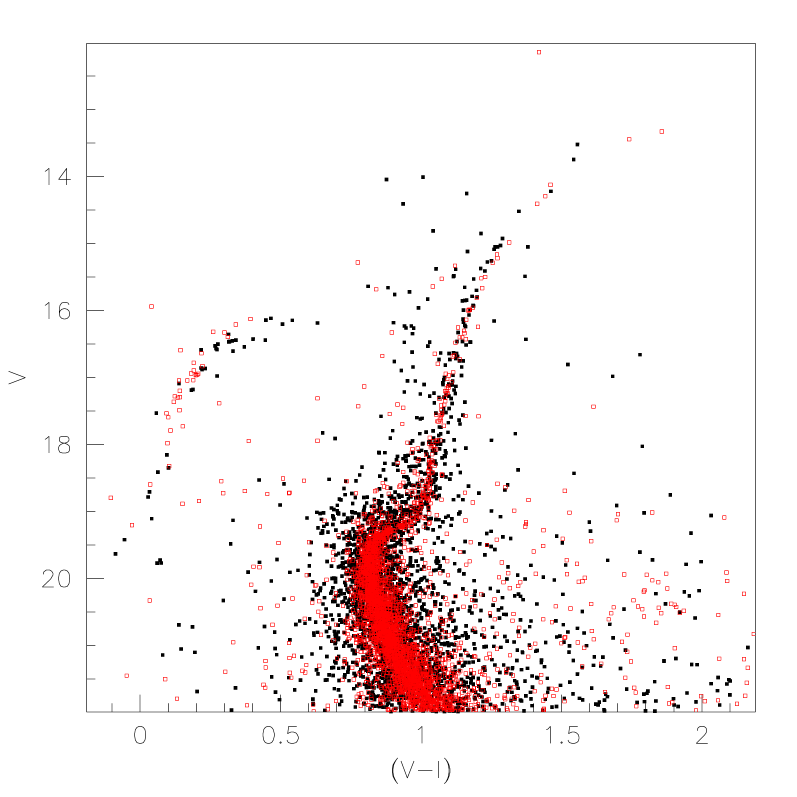
Figure 1: M80 (filled squares) vs. M12 (open squares). An offset $\delta(V-I)=-0.03$ and $\delta V=+1.50$ was applied to the M12 diagram before overlapping it to that of M80

The comparison of the observed color-magnitude diagrams (CMD) of a star cluster with the theoretical isochrones is the best tool we have to tune some fundamental parameters of the stellar evolutionary models. Only when we are sure that the input parameters and the input physics are correct, we can use the model to infer some properties of the stellar population (like age, helium content, etc.), not otherwise empirically measurable. Clearly, this is a complex job: on one side we want to use the cluster stars to tune the models, and on the other we need to use the models to infer properties of the cluster stellar population. Not surprisingly, any stellar models must adopt a number of assumptions, often not directly supported by observational evidence. One of the most uncertain parameters, strongly affecting the theoretical location of some branches of the CMD, like the red giant branch, is the mixing length parameter $\alpha$. This parameter, in the framework of the mixing-length theory (MLT; Böhm-Vitense bohm-vitense58 (1958)), determines the efficiency of energy transport by convection in the outermost layers of a star. For a given stellar luminosity, it also determines the exact radius of the star, and hence its effective temperature and colors.

It is well known that, in order to reproduce the typical temperatures and colors of red giant stars, $\alpha$ is required to have a value between 1.5 and 2.0. Also, a value close to 1.7 is required for reproducing the solar radius in non-diffusive solar models, whereas about 1.9 is favored when diffusion is taken into account. The fact that $\alpha$ is similar for red giants and the Sun (VandenBerg et al. vandenberg00 (2000); Alonso et al. alonsoEtal00 (2000)) leads to the usual approach of calibrating $\alpha$ by means of a solar model – i.e. a model with 1 $M_{\odot}$ and solar composition, that is required to have the solar luminosity and radius at an age of $\sim 4.5$ Gyr. The same $\alpha$ value is then used to model all stars, including red giants. However, there is no theoretical justification that the same value of $\alpha$ should apply for any star.

In this paper, we have attempted to investigate which is the best value of $\alpha$ for low mass (globular cluster) stars and, overall, whether there is any dependence of $\alpha$ with the cluster metallicity. Our results cannot be considered definitive; however this paper shows a possible approach to the problem, and enlightens all the uncertainties associated to the calibration of the mixing length parameter. Also, this work is limited to the context of the MLT, which is still a fundamental approach adopted in most computations of stellar models. However, one should keep in mind that the MLT is admittedly a very approximate theory, and that alternative approaches (e.g. Canuto & Mazzitelli canutomazzitelli91 (1991); Spruit spruit97 (1997); Ludwig et al. ludwigEtal99 (1999)) have been suggested.

This project has been stimulated by an investigation carried out by some of us a few years ago. In the course of a photometric study of the Galactic globular cluster (GGC) M80 (Brocato et al. brocatoEtal98 (1998), hereafter B98), we compared the morphological characteristics of its color-magnitude diagram (CMD) with those of an ensemble of other globulars for which a CMD was available in the literature. That investigation left an open question concerning the relative position of the RGB with respect to the HB as a function of the metallicity. More specifically, when the CMD of M80 was compared with that of GGCs with similar metallicity, we found a group of clusters (M3, M13, NGC 7492) whose members had CMDs overlapping that of M80, and another (M12, NGC 1904, NGC 5897) for which significant discrepancies were seen. The discrepancies were in the sense that while the HBs could be overlapped in a satisfactory way, the RGB fiducial lines showed a dispersion in color, M12 having the reddest branch (cf Fig. 6 and 7 in B98), as expected if M12 would be more metal rich than indicated in the literature. We also excluded that the discrepancy could be due to an age difference.

In order to have a more quantitative comparison among a larger sample of clusters, with different metal content, we devised a new morphological parameter with the aim of quantitatively measuring the distance in color of the RGB with respect to some fixed point on the HB. We selected as a reference point the so called “HB turn-down”(HB-TD), since it has been demonstrated that the location of this point in the CMD is largely unaffected by the cluster age, metallicity, and primordial He content (cf. the detailed discussion in B98). We fixed the HB-TD at $(B-V)_{0}=0$ and measured the RGB color at $0.5$ magnitudes brighter than the HB-TD level. As the position of the HB- TD is fixed, $W_{\rm HB}$ just shows the displacement of the RGB as a function of the metal content (cf. Fig. 10 of B98). We found that the trend with the metallicity is in the direction expected from the theoretical models, though with a large dispersion, particularly evident at intermediate metallicities ($-1.85<$[Fe/H]$<-1.50$), larger than expected on the basis of the measurement errors.

We were not able to decide whether such an evidence might simply be the consequence of the errors in the photometric calibration, or a peculiar distribution in the global metallicity of the clusters, and deferred further discussion until direct measurements of $\alpha$ elements and/or a database of CMDs with homogeneous calibration would have been available.

Such database is now available, thanks to the efforts of a number of the original investigators of B98, and we are now able to re-examine the question, taking also advantage of the new theoretical calculations that we have specifically performed for this project.

The paper is organized as follows. The datasets are presented in Sect. 2. The measurement procedures and the corrections for differential reddening are described in Sect. 2.1 and 2.2, respectively. Sect. 2.4 re-examines the original question of the trend and dispersion of $W_{\rm HB}$ as a function of metallicity.

Sect. 3 deals with the comparison of the VandenBerg et al. (vandenberg00 (2000); V00) and the Girardi et al. (girardiEtal00 (2000); G00) theoretical isochrones to the data. Due to the lower degree of sampling of the G00 isochrones, a more detailed description of the turn-down identification and its measurement is offered in Sect. 3.2.

The keys to the interpretation of the observed vs. computed trend of $W_{\rm HB}$ are offered in Sect. 4. In particular, the dependence on metallicity, mixing length, age, helium content, $\alpha$-enhancement, and the $T\mbox{${}_{\rm eff}$}$-color transformations are examined in Sects. 4.1, 4.2, 4.3, 4.4, 4.5, and 4.6.

Whether our data can be used to constrain the mixing length parameter is examined in Sect. 5. Furthermore, we suggest in Sect. 6 that the parameter can be employed as a metallicity indicator, with accuracies comparable to other more widely used photometric indices. Our summary and conclusions are given in Sect. 7.

The nomenclature deserves a final note. We will be using several symbols for our parameter throughout this paper. When talking about the parameter in a general way, we will use the old symbol $W_{\rm HB}$, but when referring to measurements specifically made for the $(B-V)$ or $(V-I)$ colors, we will use the symbols $W^{B-V}_{\rm HB}$ and $W^{V-I}_{\rm HB}$, respectively.

2 The data set

For this paper we used two new, photometrically homogeneous databases that we have recently created:

• The $V,I$ band “ground-based” dataset collected by Rosenberg et al (2000a , 2000b ) used for the GGC relative age project by Rosenberg et al. (rel-ages99 (1999));

• the “HST snapshot” dataset (Piotto et al. piottoEtal02 (2002)), based on F439W ($B$) and F555W ($V$) WFPC2 images of the core of all the GGCs with $(m-M)_{B}<18.0$, which has already been used to constrain a number of parameters in the models (Zoccali et al. zoccaliEtal00 (2000), Piotto et al. piottoEtal00 (2000), Bono et al. bonoEtal01 (2001)).

Both databases are available to the community on the Web pages of the Padova Globular Cluster Group at http://menhir.pd.astro.it.

For the present project, we used $26$ clusters in the $B,\,V$ bands from the HST snapshot database, spanning a metallicity interval $-2.2<$[Fe/H]$<-0.5$, and $31$ clusters from the ground-based dataset, in the $V,\,I$ bands, and covering a metallicity interval $-2.3<$[Fe/H]$<-1.1$.

The most important property of these databases for the aim of the present project is their photometric internal homogeneity (cf. Rosenberg et al. 2000a and 2000b , and Piotto et al. piottoEtal02 (2002)). This homogeneity removes the main uncertainty in the comparison done by B98. And, indeed, as exemplified in Fig. 1, the two new CMDs of M12 and M80 perfectly overlap, giving the first confirmation that the spread noted by B98 was mainly due to the photometric in-homogeneity of the data collected from the literature.

2.1 Measurement of the $W_{\rm HB}$ parameter

In order to compute the value of $W_{\rm HB}$, we first measured the position of the HB turn-down for each cluster, and then the color of the RGB at $0.5$ magnitudes above the HB-TD.

The HB-TD position is, using the definition of B98, the place where the true color of the HB is zero. In order to find the TD on the observed diagrams, we first defined a fiducial HB, that extends from the faint-blue tail to the bright-red clump. For the hst dataset, NGC 2808 was used, since it already satisfies our requirements (see e.g. Fig. 4 of Bedin et al. rolly00 (2000)). On the other hand, no cluster in the ground-based sample has such an extended HB, so we constructed a mean fiducial HB, following the procedure adopted in Rosenberg et al. (rel-ages99 (1999)). Briefly, we started with the HB of NGC 1851, which has a bimodal HB, and then extended it to the blue or the red by comparison with, respectively, more metal poor and more metal rich clusters.

The theoretical HBs from VandenBerg et al. (vandenberg00 (2000); see Fig. 2) were then fitted to the fiducial HBs, and the TD-HB fixed at ($B-V$)=0.0, and ($V-I$)=0.0, as in B98. For each cluster, we applied a color and a magnitude offset until a satisfying visual superposition to the reference HB was obtained (cf. Figs. 3, 4). Finally the TD color and magnitude for each cluster are those of the mean fiducial plus the two offsets. A special case is that of NGC 6388 and NGC 6441, whose HBs are evidently sloped, such that the blue portion just before the HB-TD is brighter than the red portion (see Piotto et al. piottoEtal02 (2002)). There are enough stars on the blue side, around the HB-TD, to allow a determination of the HB-TD position, without relying on the red part of the HB. However, if we tried to reach an overall agreement from blue to red, then a slightly fainter HB-TD would have been found. In turn, this implies a smaller $W_{\rm HB}$, and one can see in Fig. 7 and the following, that the representative points of the two cluster would move toward the general trend defined by the isochrones.

Figure 2: The TD position is shown on the V00 theoretical HBs in the case of the $(B-V)$ color (upper panel) and $(V-I)$ color (lower panel). Each line corresponds to the theoretical ZAHB sequence for a given metallicity. Each one of them has been vertically shifted in this plot, so that they all coincide at the TD point. In the two panels, the empirical fiducial HBs have been represented as well. They can be recognized as the solid curves ending at colors $\approx 0.7$, and slightly fainter than the theoretical loci.

Figure 3: An example of measurement of $W^{B-V}_{\rm HB}$, for NGC 5694. This figure shows the mean fiducial HB in $(B-V),V$ (large open circles), the position of the TD, and the corresponding color of the point on the RGB which is $0.5$ magnitudes brighter than the TD. The inset shows the histogram of the color distribution on the RGB, and the solid curve is a Gaussian computed assuming the calculated mean and dispersion of the data.

Figure 4: Same as Fig. 3, showing an example of measurement of $W^{V-I}_{\rm HB}$ for NGC 6656.

In order to measure the color of the RGB, we first obtained by hand an approximate color of the RGB region $0.5$ magnitude brighter than the TD level. The final color was computed as the median color of all the stars comprised in a rectangular region around this first RGB position estimate. The box dimensions were slightly varied from cluster to cluster, so that the whole RGB color extension was comprised. The “vertical” size was chosen as to ensure that a statistically significant number of stars entered the computation. Typical values are $0.06$ magnitudes in color and $0.12$ magnitudes in $V$. The Figs. 3 and 4 show the final step of the procedure for NGC 5694 (HST data) and NGC 6656 (groundbased data).

2.2 Correction for differential reddening

Since $W_{\rm HB}$ represents a difference in color, and since the two points are about $1$ magnitude apart, we cannot neglect the effect of the wavelength dependence of the reddening. It is known that, given a mean reddening $E_{B-V}$, the value of the absorption $A_{V}=R_{V}\times E_{B-V}$ varies with the star color (temperature). In the case of heavily reddened clusters, we must also take into account the dependence of $R_{V}$ on the absolute reddening $E_{B-V}$.

A first investigation on these effects was carried out by Olson (Olso75 (1975)), who proposed a correction for the $(B-V)$ color. Later, Grebel and Roberts (greb95 (1995); GR95) extended this study by determining the trends of $R$, $A_{V}$, colors, and reddenings, not only as a function of the temperature, but also on star’s gravity and metallicity. The results of GR95 are consistent with Olson (Olso75 (1975)).

We used the results from both studies to correct the $W_{\rm HB}$ parameter measured in the $B,\,V$ bands. In order to correct the $W_{\rm HB}$ parameter obtained in the $V$ vs. $(V-I)$ CMD, we used the GR95 tables, thus ensuring the homogeneity of the results. More details on our calculations are given in Appendix A.

2.3 Metallicity scales

Most values of the iron abundance for the single clusters have been taken from Rutledge et al. (rhs97 (1997); RHS97). More explicitly, we have taken the [Fe/H] values that RHS97 obtained by calibrating their CaII triplet equivalent widths onto either the Zinn & West (zinnWest84 (1984); ZW84) or the Carretta & Gratton (carrettaGratton97 (1997); CG97) metallicity scales. For a few clusters, there are no estimates of the metallicity provided by RHS97, and in such cases the [Fe/H] values on the ZW84 scale are from Harris (harris96 (1996)), and from Carretta (private communication) for the CG97 scale. We have attached a typical error of $0.15$ dex to the metallicities in this class.

2.4 The $W_{\rm HB}$ parameter vs. metallicity

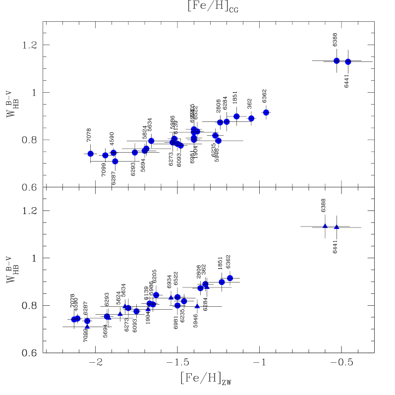
Figure 5: All the data for $W^{B-V}_{\rm HB}$, as a function of metallicity, adopting the CG97 (top panel) or ZW84 (bottom panel) metallicity scales. Filled triangles identify clusters whose metallicity on the ZW84 scale has been taken from Harris (harris96 (1996)).

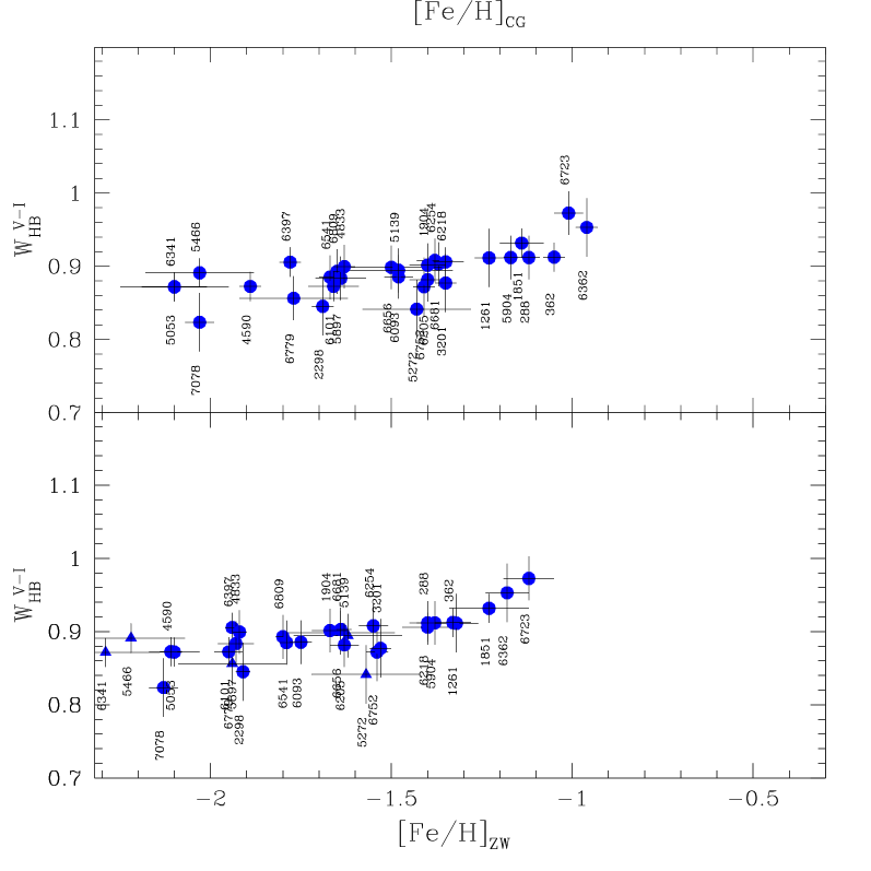
Figure 6: The same as Fig. 5, but for $W^{V-I}_{\rm HB}$.

As in B98, Figs. 5 and 6 display the $W^{B-V}_{\rm HB}$ and $W^{V-I}_{\rm HB}$ parameters as a function of [Fe/H], both on the Zinn and West (zinnWest84 (1984), lower panel) and the Carretta and Gratton (carrettaGratton97 (1997), upper panel) metallicity scales. The same data is presented in Table 1. The first remarkable result, at variance with B98, is the low dispersion of the data points, fully compatible with the error bars. The dispersion at intermediate metallicities noted in B98, is no longer present. As originally suspected, the anomalous trend in the B98 data was likely due to calibration errors present in their CMD database, which was a simple collection of literature data. Again, this result shows the importance of using a photometric homogeneous database in deriving the properties of the stellar population of star clusters.

Table 1: Measured values of $W_{\rm HB}$ for our sample. An underlined $0.15$ dex error in the metallicity, highlights a value of the [Fe/H] taken from Harris (harris96 (1996)).

Id.	[Fe/H]ZW	[Fe/H]CG	$W^{B-V}_{\rm HB}$
NGC 362	$-1.33\pm 0.05$	$-1.05\pm 0.03$	$0.88\pm 0.03$
NGC 1851	$-1.23\pm 0.11$	$-1.14\pm 0.06$	$0.89\pm 0.04$
NGC 1904	$-1.67\pm 0.05$	$-1.40\pm 0.05$	$0.80\pm 0.03$
NGC 2808	$-1.36\pm 0.05$	$-1.24\pm 0.03$	$0.87\pm 0.03$
NGC 4590	$-2.11\pm 0.03$	$-1.89\pm 0.03$	$0.74\pm 0.02$
NGC 5634	$-1.82\pm\underline{0.15}$	$-1.66\pm\underline{0.15}$	$0.79\pm 0.03$
NGC 5694	$-1.93\pm 0.04$	$-1.70\pm 0.07$	$0.75\pm 0.03$
NGC 5824	$-1.85\pm\underline{0.15}$	$-1.69\pm\underline{0.15}$	$0.76\pm 0.03$
NGC 5946	$-1.38\pm\underline{0.15}$	$-1.25\pm\underline{0.15}$	$0.79\pm 0.03$
NGC 5986	$-1.65\pm 0.04$	$-1.52\pm 0.04$	$0.80\pm 0.03$
NGC 6093	$-1.75\pm 0.03$	$-1.48\pm 0.04$	$0.77\pm 0.03$
NGC 6139	$-1.68\pm\underline{0.15}$	$-1.50\pm\underline{0.15}$	$0.78\pm 0.03$
NGC 6205	$-1.63\pm 0.04$	$-1.40\pm 0.05$	$0.84\pm 0.04$
NGC 6235	$-1.46\pm 0.06$	$-1.27\pm 0.05$	$0.81\pm 0.03$
NGC 6273	$-1.80\pm 0.03$	$-1.53\pm 0.05$	$0.78\pm 0.04$
NGC 6284	$-1.32\pm\underline{0.15}$	$-1.20\pm\underline{0.15}$	$0.87\pm 0.04$
NGC 6287	$-2.05\pm\underline{0.15}$	$-1.88\pm\underline{0.15}$	$0.70\pm 0.04$
NGC 6293	$-1.92\pm\underline{0.15}$	$-1.76\pm\underline{0.15}$	$0.74\pm 0.04$
NGC 6362	$-1.18\pm 0.06$	$-0.96\pm 0.03$	$0.91\pm 0.03$
NGC 6388	$-0.60\pm\underline{0.15}$	$-0.53\pm\underline{0.15}$	$1.13\pm 0.05$
NGC 6441	$-0.53\pm\underline{0.15}$	$-0.46\pm\underline{0.15}$	$1.12\pm 0.05$
NGC 6522	$-1.50\pm 0.05$	$-1.38\pm 0.04$	$0.83\pm 0.04$
NGC 6934	$-1.54\pm\underline{0.15}$	$-1.40\pm\underline{0.15}$	$0.83\pm 0.03$
NGC 6981	$-1.50\pm 0.05$	$-1.40\pm 0.04$	$0.79\pm 0.04$
NGC 7078	$-2.13\pm 0.04$	$-2.03\pm 0.04$	$0.74\pm 0.04$
NGC 7099	$-2.05\pm 0.03$	$-1.94\pm 0.04$	$0.73\pm 0.03$
Id.	[Fe/H]ZW	[Fe/H]CG	$W^{V-I}_{\rm HB}$
NGC 288	$-1.40\pm 0.05$	$-1.12\pm 0.03$	$0.91\pm 0.03$
NGC 362	$-1.33\pm 0.05$	$-1.05\pm 0.03$	$0.91\pm 0.02$
NGC 1261	$-1.32\pm 0.06$	$-1.23\pm 0.04$	$0.91\pm 0.04$
NGC 1851	$-1.23\pm 0.11$	$-1.14\pm 0.06$	$0.93\pm 0.02$
NGC 1904	$-1.67\pm 0.05$	$-1.40\pm 0.05$	$0.90\pm 0.03$
NGC 2298	$-1.91\pm 0.02$	$-1.69\pm 0.03$	$0.84\pm 0.04$
NGC 3201	$-1.53\pm 0.03$	$-1.35\pm 0.03$	$0.87\pm 0.04$
NGC 4590	$-2.11\pm 0.03$	$-1.89\pm 0.03$	$0.87\pm 0.02$
NGC 4833	$-1.92\pm 0.02$	$-1.63\pm 0.03$	$0.89\pm 0.03$
NGC 5053	$-2.10\pm 0.07$	$-2.10\pm 0.09$	$0.87\pm 0.02$
NGC 5139	$-1.62\pm\underline{0.15}$	$-1.48\pm\underline{0.15}$	$0.89\pm 0.03$
NGC 5272	$-1.57\pm\underline{0.15}$	$-1.43\pm\underline{0.15}$	$0.84\pm 0.04$
NGC 5466	$-2.22\pm\underline{0.15}$	$-2.03\pm\underline{0.15}$	$0.89\pm 0.02$
NGC 5897	$-1.93\pm 0.05$	$-1.64\pm 0.07$	$0.88\pm 0.03$
NGC 5904	$-1.38\pm 0.05$	$-1.17\pm 0.02$	$0.91\pm 0.03$
NGC 6093	$-1.75\pm 0.03$	$-1.48\pm 0.04$	$0.88\pm 0.03$
NGC 6101	$-1.95\pm 0.04$	$-1.66\pm 0.07$	$0.87\pm 0.02$
NGC 6205	$-1.63\pm 0.04$	$-1.40\pm 0.05$	$0.88\pm 0.03$
NGC 6218	$-1.40\pm 0.07$	$-1.35\pm 0.05$	$0.90\pm 0.02$
NGC 6254	$-1.55\pm 0.04$	$-1.38\pm 0.05$	$0.90\pm 0.03$
NGC 6341	$-2.29\pm\underline{0.15}$	$-2.10\pm\underline{0.15}$	$0.87\pm 0.02$
NGC 6362	$-1.18\pm 0.06$	$-0.96\pm 0.03$	$0.95\pm 0.04$
NGC 6397	$-1.94\pm 0.02$	$-1.78\pm 0.03$	$0.90\pm 0.02$
NGC 6541	$-1.79\pm 0.02$	$-1.67\pm 0.03$	$0.88\pm 0.03$
NGC 6656	$-1.64\pm\underline{0.15}$	$-1.50\pm\underline{0.15}$	$0.89\pm 0.03$
NGC 6681	$-1.64\pm 0.03$	$-1.37\pm 0.03$	$0.90\pm 0.03$
NGC 6723	$-1.12\pm 0.07$	$-1.01\pm 0.04$	$0.97\pm 0.03$
NGC 6752	$-1.54\pm 0.03$	$-1.41\pm 0.03$	$0.87\pm 0.04$
NGC 6779	$-1.94\pm\underline{0.15}$	$-1.77\pm\underline{0.15}$	$0.85\pm 0.03$
NGC 6809	$-1.80\pm 0.02$	$-1.65\pm 0.03$	$0.89\pm 0.03$
NGC 7078	$-2.13\pm 0.04$	$-2.03\pm 0.04$	$0.82\pm 0.04$

The linear dependence of $W_{\rm HB}$ on metallicity suggested by B98 is not confirmed by Figs. 5 and 6: there is a break in the linear trend at about [Fe/H]$\sim-1.4$. This is more evident for $W^{B-V}_{\rm HB}$, thanks to the larger coverage in metallicity of the HST data.

Figs. 5 and 6, shows also that a given change in [Fe/H] produces a change in $W^{B-V}_{\rm HB}$ which is $\sim 1.5$ times larger than that in $W^{V-I}_{\rm HB}$.

3 Comparison with theoretical models

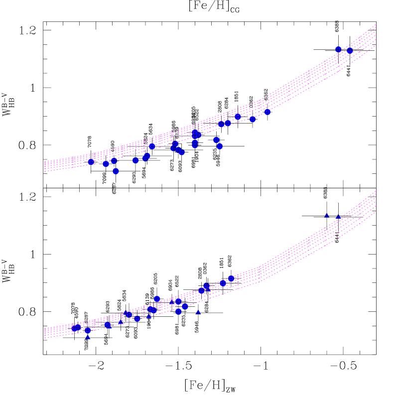
Figure 7: $W_{\rm HB}^{(B-V)}$ as a function of metallicity, using the hst data sample. The CG97 scale is used in the top panel, while ZW84 is used in the lower one. The dashed lines reproduce the theoretical parameter calculated using the V00 isochrones, between ${8\textrm{ Gyr}}$ (lower line) and ${18\textrm{ Gyr}}$ (upper line), and in $2$ Gyr steps.

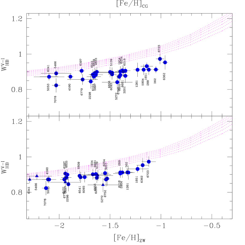
Figure 8: Same as Fig. 7, for the ground-based dataset.

The interpretation of the data was carried out using both the VandenBerg et al. (vandenberg00 (2000)) and Girardi et al. (girardiEtal00 (2000)) isochrones.

We first present the two isochrone sets, and then show the theoretical prediction for $W_{\rm HB}$ vs. [Fe/H] together with the empirical data sets. The thorough inter-comparison is then carried out in Sect. 4.

3.1 The VandenBerg et al. (vandenberg00 (2000)) isochrones

The V00 isochrones are computed for $17$ values of [Fe/H] ($-2.3\leq\rm[Fe/H]\leq-0.3$), $6$ age values ($8\leq t\leq 18$ Gyr), and a fixed mixing length parameter $\alpha_{\rm MLT}=1.89$. These models were computed for a fixed value of [$\alpha$/Fe]$=0.3$, where $\alpha$ stands for the alpha-elements O, Ne, Na, Mg, Si, S, Ar, Ca and Ti. The isochrones have been transformed to the observational plane by means of semi-empirical color-$T\mbox{${}_{\rm eff}$}$ relations (see VandenBerg et al. vandenberg00 (2000)) that are essentially theoretical for $\mbox{$T\mbox{${}_{\rm eff}$}$}>5000$ K (where the TD is), and empirically-corrected for lower $T\mbox{${}_{\rm eff}$}$ s (where the RGBs are).

The V00 database includes smooth and well-behaved ZAHB sequences for all their metallicity values. They are shown in Fig. 2, for both the $B-V$ and the $V-I$ colors. All ZAHB sequences have been shifted vertically in this plot, so that they coincide at the point where the color is 0, i.e. at the turn-down. No color shift has been applied, further confirming that the HB-TD point is fixed in color. This figure has also been used to define the “mean HB” mentioned previously in Sect. 2.1.

The trends with metallicity of $W_{\rm HB}^{B-V}$ and $W_{\rm HB}^{V-I}$ from V00 models (dashed lines) are compared with the data in Figs. 7 and 8, respectively. As it can be noticed, these models reproduce reasonably well the data for $W_{\rm HB}^{B-V}$, especially if the ZW scale is adopted, but present $W_{\rm HB}^{V-I}$ values that are systematically larger than the observed ones by about 0.1 mag. This point is thoroughly discussed in Sect. 4. It is also clear that $W_{\rm HB}$ increases with age, since the Hayashi track becomes redder as the mass of evolved giants decrease (see also Sect. 4.3).

3.2 The Girardi et al. (girardiEtal00 (2000)) isochrones

The G00 models were calculated for metallicities $Z=0.0004$, $0.001$, $0.004$, $0.008$, $0.019$ and $0.03$ (Girardi et al. girardiEtal00 (2000)). An additional set with $Z=0.0001$ (or [Fe/H]$=-2.28$) has been computed adopting identical input physics (Girardi, unpublished). All models have been computed with scaled-solar metal ratios and a helium content that mildly increases with $Z$, i.e. $Y=0.23+2.75\,Z$. In this case, the relation $\mbox{[Fe/H]}=\log(Z/0.019)$ gives [Fe/H] values accurate to within 0.03 dex. Thus, the 5 lowest $Z$ values we are going to consider (0.0001, 0.0004, 0.001, 0.004, and 0.008) would correspond to [Fe/H] values of $-2.28$, $-1.68$, $-1.28$, $-0.68$, and $-0.38$. The mixing length parameter was assumed to be $\alpha_{\rm MLT}=1.68$.

The Girardi et al. (girardiEtal00 (2000)) models are computed with OPAL (Rogers & Iglesias rogersIglesias92 (1992)) and Alexander & Ferguson (alexanderFerguson94 (1994)) opacities, and an updated equation of state that considers the main non-ideal effects, such as the Debye-Huckel correction. In these aspects, their lowest-mass models (oldest isochrones) are very similar to many of the non-diffusive stellar models available in the literature (see e.g. Weiss & Schlattl weissSchalttl98 (1998)). However, due to small differences in the adopted physics of electron-degenerate matter, and in the way used to generate ZAHB structures, Girardi et al. models present ZAHB luminosities that are systematically lower (by $\sim 0.2$ mag) than other recent calculations (see Castellani et al. castellaniEtal00 (2000), and Salasnich 2001, for all details). These difference in luminosity seems to be systematic and almost independent of metallicity: in fact, G00 ZAHB models obey the relation $M_{V}^{\textrm{RRLyr}}=(0.163\pm 0.015)\,\mbox{[Fe/H]}+{\textrm{constant}.}$ (see Salasnich salasnich01 (2001)), whose slope is consistent with those typically found in most recent models of stellar evolution, i.e. $0.18\leavevmode\nobreak\ \rm mag/dex$ (e.g. Cassisi et al. cassisiEtal99 (1999)).

Figure 9: ZAHB sequences from G00 models.

The G00 core-helium burning models are quite complete and well-sampled for masses higher than 0.6 $M_{\odot}$. For lower masses, the ZAHB is not as well covered as in V00 models and, as a consequence, the identification of the HB-TD is not as straightforward. To this aim, we proceeded in the following way: First, we artificially obtained a more detailed ZAHB sequence in the HR diagram, by simply interpolating between the ZAHB models that have been actually calculated for just a few masses $M<0.6$ $M_{\odot}$. This is displayed in the upper panel of Fig. 9. As it can be noticed, the computed models are disposed along sequences that are fairly linear in the temperature interval $\log\mbox{$T\mbox{${}_{\rm eff}$}$}>3.8$. Thus, we can safely adopt linear interpolations between these different models. Also the mass values are linearly interpolated, which represents a less accurate, but not critical, approximation.

Then, the interpolated ZAHB sequences are transformed to the observational quantities by adopting the metallicity-dependent bolometric corrections and color transformations from Bertelli et al. (bertelliEtal94 (1994)). In the $T\mbox{${}_{\rm eff}$}$ interval we are dealing with, these transformations are entirely based on Kurucz’ (kurukz92 (1992)) library of synthetic spectra. They are mainly a function of $T\mbox{${}_{\rm eff}$}$  and just marginally depend on the surface gravity $g$. Thus, any possible inadequacy in the interpolation of stellar masses would not be critical in this step.

The results for the $M_{V}$ vs. $B\!-\!V$ and $M_{V}$ vs. $V\!-\!I$ diagrams are shown in the middle and lower panels of Fig. 9, respectively. Looking at this figure, one can notice that the ZAHB sequences of lower metallicities are systematically shifted to lower (brighter) magnitudes.

The position of the turn-down is largely determined by the behavior of the $V$-band bolometric corrections as a function of either $T\mbox{${}_{\rm eff}$}$ or color. We define the turn-down as the point of each ZAHB sequence for which $\mbox{$B\!-\!V$}=0$ (in the case of $M_{V}$ vs. $B\!-\!V$ diagrams), or $\mbox{$V\!-\!I$}=0$ (for $M_{V}$ vs. $V\!-\!I$ diagrams). Since the zero-points of the “theoretical” photometry are such that $\mbox{$B\!-\!V$}=\mbox{$V\!-\!I$}=0$ for the A0 dwarf Vega, for giants of $\mbox{$B\!-\!V$}\sim 0$ the differences between $B\!-\!V$ and $V\!-\!I$ are of just of a few hundredths of magnitude. Hence, in practice, the two different definitions of the turn-down correspond to almost (but not exactly) the same ZAHB star.

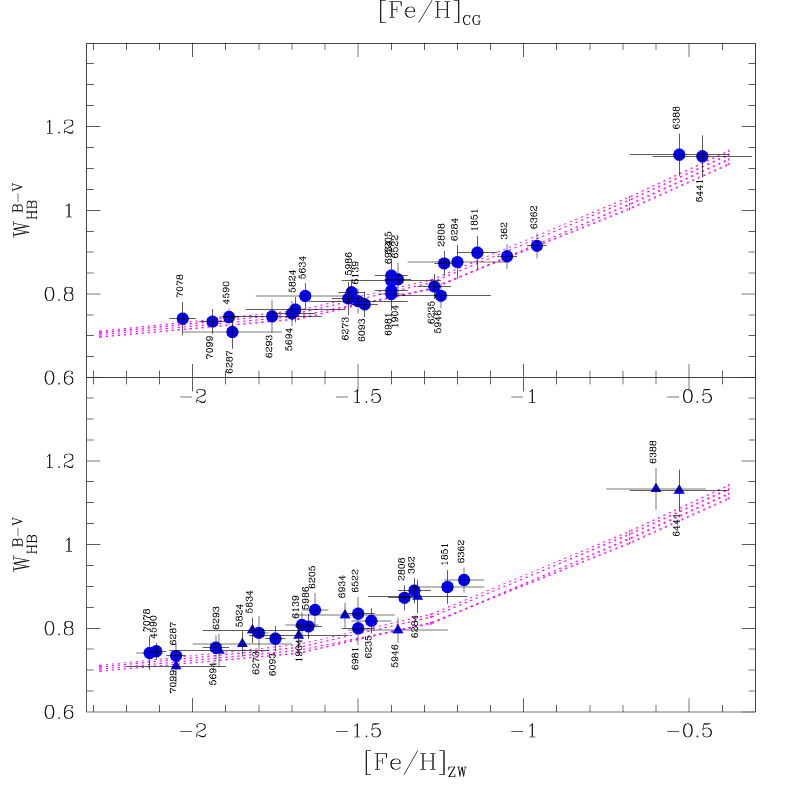
Figure 10: The $W_{\rm HB}^{B-V}$ values, as measured from our cluster sample (full dots with error bars, and marked with the clusters’ NGC number), are compared with the values derived from Girardi et al. (girardiEtal00 (2000)) isochrones (dashed lines). Going from above to below, isochrone ages are 16, 14, 12, and 10 Gyr.

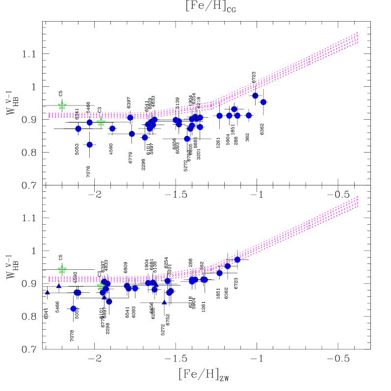
Figure 11: The same as in Fig. 10, but for $W_{\rm HB}^{V-I}$

Having defined the ZAHB turn-down position for all metallicities, for any isochrone we can measure $W_{\rm HB}^{B-V}$ and $W_{\rm HB}^{V-I}$ by simply identifying the color of the point along the RGB that is 0.5 mag brighter (in the $V$-band) than its respective turn-down. The results for $W_{\rm HB}^{B-V}$ are shown in Fig. 10, where the theoretical values obtained for isochrones with ages between 10 and 16 Gyr are compared to the observational data from Sect. 2. It can be noticed that $W_{\rm HB}^{B-V}$ values increase steadily with metallicity, following the color shift of the RGB. If the Carretta & Gratton (carrettaGratton97 (1997)) metallicity scale is adopted, we find a remarkable agreement between models and observations throughout the complete metallicity range. The agreement becomes less satisfactory if the data are plotted against the Zinn & West (zinnWest84 (1984)) metallicity scale.

Similarly, the results for $W_{\rm HB}^{V-I}$ are shown in Fig. 11. Again, $W_{\rm HB}^{V-I}$ values are found to increase steadily with metallicity in a way similar to the one present in the data, though (i) in this case, there is no data with $\mbox{[Fe/H]}>-1$ to compare the models with; and (ii) theoretical $W_{\rm HB}^{V-I}$ values are systematically larger than the data, by about $0.05$ mag .

4 What determines $W_{\rm HB}$

In this section, we will analyze the main parameters affecting the theoretical value of $W_{\rm HB}$.

The four Figs. 7, 8, 10, and 11, give us a chance to inter-compare two recent sets of theoretical calculations with empirical data. It is evident from the figures that both sets of isochrones reproduce satisfactorily the trend of the observed points as a function of [Fe/H]. The agreement is better for the $BV$ data.

For $VI$, there is a disagreement of $\sim 0.05$ magnitudes between the models and the data, which can be interpreted in two ways. Either the models predict a smaller $W_{\rm HB}$ value than observed, or there is a problem with our measurements. Before proceeding further with the discussion, we need to rule out the latter possibility. First, we notice that the offset in color is independent of the cluster reddening, so it cannot be attributed to our differential reddening corrections. Then since $W_{\rm HB}$ is a differential quantity, the only justification for such a spurious result would be the neglecting of the quadratic (and higher order) terms in the calibration equations obtained by Rosenberg et al. (2000a ; 2000b ), such that a stretch of $0.05$ magnitudes over a range of $1$ magnitude in color is produced. However, the residual scatter around the assumed linear relations was a few $0.001$ magnitudes over a range in color of more than $1.5$ magnitudes for the standard stars, so we must conclude that the problem is indeed in the synthetic colors.

The main point that emerges from these figures, therefore, is that theoretical models seem to describe reasonably well the relative position of the HB-TD and RGB, apart from a possible zero point difference in $V-I$. Since the HB-TD color is constant, Figs. 7, 8, 10, and 11 in fact represent the behavior of the RGB color, at about the HB level, as a function of metallicity.

It is well-known that the RGB color in stellar models depends on a series of factors. First of all, it depends on metallicity. Then, it should strongly depend on the efficiency of the energy transport in convective envelopes, and hence on the mixing length parameter $\alpha$. There must also be a weak dependence on the stellar mass, and hence on the adopted isochrone age. Some dependence on the model chemistry (helium content and degree of $\alpha$-enhancement) may be present. Finally, the RGB color depends on the adopted transformations between $T\mbox{${}_{\rm eff}$}$ and color. In the following, we will explore these dependencies in order to verify whether the $W_{\rm HB}$ parameter is of some usefulness in setting one of the above parameters.

4.1 Dependence of $W_{\rm HB}$ on metallicity

The dependence on the metallicity of $W_{\rm HB}$ is the most obvious and the strongest one. It is clearly visible in Figs. 3 and 4. As the metallicity increases, the RGB becomes redder and redder, while we do not expect a variation in the HB-TD color, and therefore $W_{\rm HB}$ increases. The effect is stronger in ($B-V$) than in ($V-I$). We will discuss this dependence in more details in Sect. 6.

4.2 Dependence of $W_{\rm HB}$ on the mixing length parameter $\alpha$

Among the various parameters fixing the RGB position, the mixing length parameter $\alpha$ plays one of the main roles, since in RGB stars a significant fraction of the energy flux is transported by convection. The larger the value of $\alpha$, the higher the temperature of the RGB.

In order to evaluate the effect of $\alpha$ in the $W_{\rm HB}$ parameter, we computed an additional set of stellar models, from the zero age main sequence (ZAMS) up to the He-flash, for $\alpha$ equal to 1.30 and 2.00, respectively. Only stars of 0.8 $M_{\odot}$ were considered; this mass value is close the one found in the upper RGB of isochrones that are 10 to 15 Gyr old. Together with the set of $\alpha=1.68$ tracks already available (G00), the new tracks allow us to evaluate how $W_{\rm HB}^{B-V}$ and $W_{\rm HB}^{V-I}$ change as a function of $\alpha$. The $W_{\rm HB}^{B-V}$ and $W_{\rm HB}^{V-I}$ values for all our models with 0.8 $M_{\odot}$, are plotted in Figs. 12 and 13, together with the values derived from our $10-16$ Gyr old isochrones.

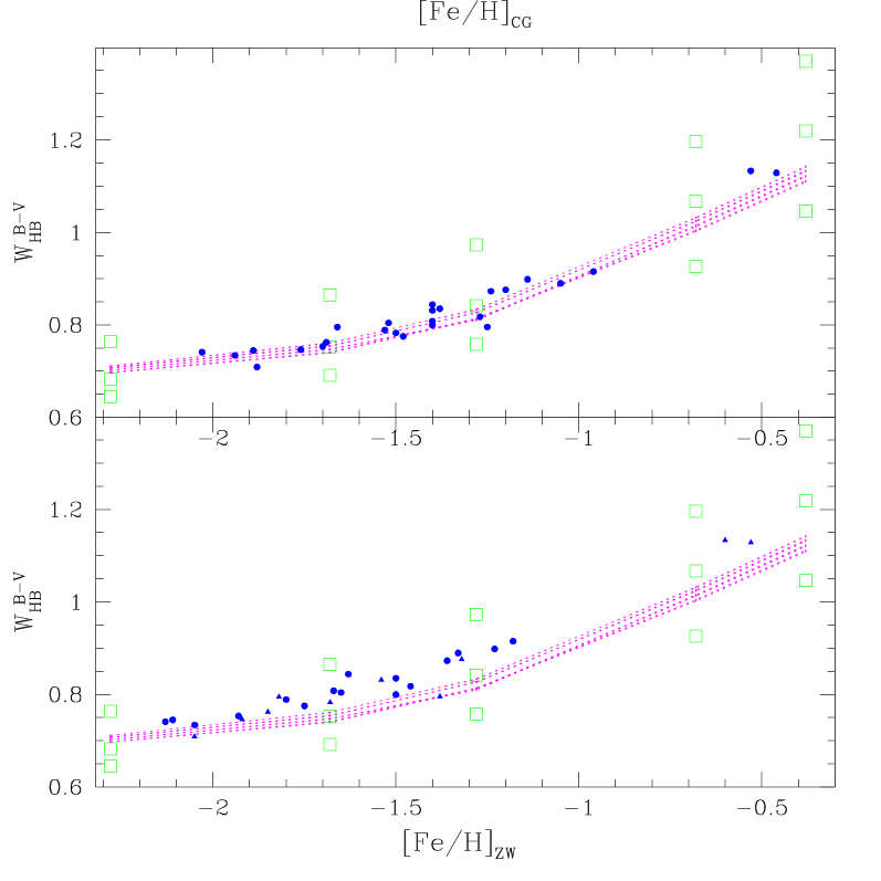
Figure 12: Open squares: $W_{\rm HB}^{B-V}$ values measured for a set of 0.8 $M_{\odot}$ evolutionary tracks of varying metallicity and mixing length parameter $\alpha$. For each metallicity, $\alpha$ values are 1.30, 1.68, and 2.00, going from above to below. For the sake of comparison, we also plot the $W_{\rm HB}^{B-V}$ values as derived from the same isochrones as in Fig. 10 (dashed lines), and the observational values for our cluster sample (small dots).

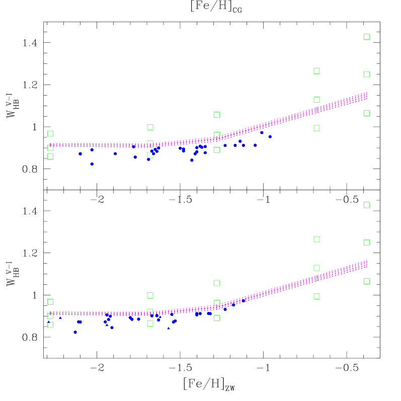
Figure 13: The same as in Fig. 12, but for $W_{\rm HB}^{V-I}$.

It can be noticed that, for lower metallicities, the points corresponding to 0.8 $M_{\odot}$, $\alpha=1.68$ models, coincide with the locus of the isochrones. For higher metallicities, this does not happen, since metal-rich $10-16$ Gyr isochrones typically present RGB stars of higher masses ($0.9-1.0$ $M_{\odot}$), and hence hotter and bluer than 0.8 $M_{\odot}$ RGB stars.

Other points to be noticed are that: (i) Models calculated with different $\alpha$ present virtually the same value of core mass at the helium flash as the $\alpha=1.68$ ones, and a similar amount of dredged-up helium. This implies that the ZAHB models derived from these tracks would present essentially the same luminosities. (ii) Stars hotter than $\mbox{$T\mbox{${}_{\rm eff}$}$}\simeq 7000$ K have their radii essentially insensitive to the treatment of the outer convection, and therefore independent of $\alpha$ (see Renzini & Fusi Pecci renziniFusipecci88 (1988); and figure 1 in Castellani et al. castellaniEtal99 (1999)). Hence, even if we did not compute ZAHB models with different $\alpha$ values, we know that the HB-TD position would not have changed.

Then, we can use the computed 0.8 $M_{\odot}$ RGB models to derive the dependence of $W_{\rm HB}$ on $\alpha$: For each metallicity, we have fitted straight lines to the $W_{\rm HB}^{B-V}$ versus $\alpha$, and $W_{\rm HB}^{V-I}$ versus $\alpha$ data, using the 3 RGB tracks we have for each metallicity. In all cases, the linear fit produced an excellent description of the data. Therefore, we can conclude that the $W_{\rm HB}^{B-V}(\alpha)$, and $W_{\rm HB}^{V-I}(\alpha)$ relations are very much linear. The slopes of the fitted lines, $\Delta W_{\rm HB}^{B-V}/\Delta\alpha$ and $\Delta W_{\rm HB}^{V-I}/\Delta\alpha$, are presented in Table 2, for each [Fe/H].

Table 2: Derivatives of $W_{\rm HB}$ cf. G00 models.

$Z$	$\Delta W_{\rm HB}^{B-V}/\Delta\alpha$	$\Delta W_{\rm HB}^{B-V}/\Delta({\rm age})$	$\Delta(B-V)_{\rm RGB}$	$\Delta W_{\rm HB}^{V-I}/\Delta\alpha$	$\Delta W_{\rm HB}^{V-I}/\Delta({\rm age})$	$\Delta(V-I)_{\rm RGB}$
		$({\rm Gyr}^{-1})$	(Alonso$-$Kurucz)		$({\rm Gyr}^{-1})$	(Alonso$-$Kurucz)
$0.0001$	$-0.17$	$0.0026$	–	$-0.16$	$0.0020$	–
$0.0004$	$-0.25$	$0.0036$	–	$-0.19$	$0.0025$	$-0.046$
$0.001$	$-0.31$	$0.0038$	–	$-0.24$	$0.0018$	$-0.050$
$0.004$	$-0.38$	$0.0053$	$0.175$	$-0.39$	$0.0040$	$-0.039$
$0.008$	$-0.46$	$0.0057$	$0.105$	$-0.52$	$0.0045$	$-0.033$

The numbers in Table 2 confirm the strong dependence of $W_{\rm HB}$ on $\alpha$, to be compared with the much lower dependence on age.

4.3 Dependence of $W_{\rm HB}$ on age

The dependence of $W_{\rm HB}$ on age is already illustrated in Figs. 7, 8, 10, and 11, where isocrohones for a wide range of ages are presented. In Table 2, instead, we tabulate the derivatives of $W_{\rm HB}$ with respect to age, at 14 Gyr, as derived from G00 models. Surprisingly, in V00 models these derivatives are about twice as large; but anyway, it is clear that $W_{\rm HB}$ changes very little with age. Taking into account the small age dispersion found by Rosenberg et al. (rel-ages99 (1999)) for the same clusters used in the present investigation, we conclude that the effects of age variations from cluster to cluster are much smaller than the error bars of the single data points.

4.4 Dependence of $W_{\rm HB}$ on the helium content

When the helium content is increased, the HB luminosity also increases according to the law $\Delta V/\Delta Y=-3.22$ for $0.23<Y<0.27$, i.e. the values suggested by current observations ($R$ parameter, HII regions, etc.). This means that, when measuring $W_{\rm HB}$, we will consider a brighter RGB point as well. This point will be redder, whereas the HB-TD does not change in color, so the net result is that increasing $Y$ will lead to a larger $W_{\rm HB}$. The size of this effect was measured using a $12$ Gyr isochrone from V00, varying [Fe/H] in the whole range, and for five values of $Y$.

The comparison with the observations is shown in Figs. 14 and 15, for the hst and ground-based samples, respectively.

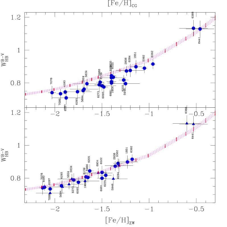
Figure 14: The dashed lines show the effect, on $W^{B-V}_{\rm HB}$, of varying the helium content on the theoretical models. See text for the explanation.

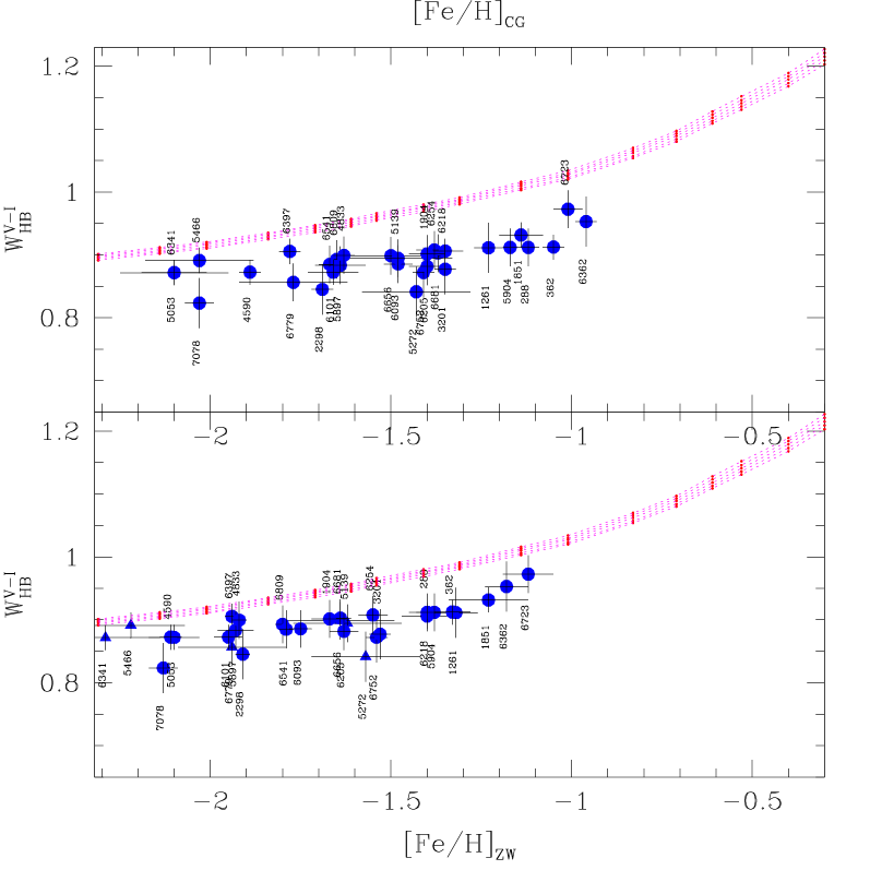
Figure 15: Same as Fig. 14, for the ground-based observations.

The figures show that, while there is a zero-point problem (which could be solved changing the reference age), the relative trend is well reproduced by the models. In any case, variations in helium content have a negligible effect on $W_{\rm HB}$. The dispersion of the empirical points due to the observational uncertainties is larger than the dispersion we would expect from a reasonable cluster to cluster variations in the helium content. Therefore, we conclude that the dependence of $W_{\rm HB}$ on the He mass fraction can be ignored.

4.5 Dependence of $W_{\rm HB}$ on $\alpha$-enhanced metal ratios

Halo populations are expected to present $\alpha$-enhanced metal ratios, with $[\alpha/{\textrm{Fe}}]\simeq 0.3$ dex. For a given metal fraction $Z$, $\alpha$-enhanced models have an iron content [Fe/H] that is depleted by a factor that corresponds roughly to the degree of enhancement $[\alpha/{\textrm{Fe}}]$. Moreover, for sufficiently low metallicities, $\alpha$-enhanced evolutionary tracks can be replaced by their scaled-solar counterparts of same $Z$ (see Salaris et al. salarisEtal93 (1996); Salaris & Weiss salarisWeiss98 (1998)).

Therefore, for low metallicities we can expect that models with solar-scaled abundances could be used to reproduce $\alpha$-enhanced isochrones, provided that their [Fe/H] values are changed by about $-0.3$ dex. Of course, this is only a first-order approximation to the question, especially for the models of higher metallicities ($\mbox{[Fe/H]}\ga 0.004$, see Salasnich et al. salasnichEtal00 (2000)). Another approximation is in the fact that the $T\mbox{${}_{\rm eff}$}$-color transformations in use have been derived from model atmospheres of scaled-solar composition, and not from $\alpha$-enhanced ones (which are not yet available). Whether this is critical, is yet to be investigated.

Keeping these points in mind, we can now get some insight on how much $W_{\rm HB}$ depends on the $\alpha$-enhancement, by taking advantage of the fact that V00 isochrones are enhanced while those of G00 are not. As a caveat, we must stress that ideally one would like to measure the size of the effect on otherwise identical models, since e.g. different color transformations could mask the true trend. As a first order approach, we will nevertheless try to understand what happens if we interpret the differences in the two isochrone sets purely in terms of $\alpha$-enhancement (i.e. as just an offset along the abscissae).

Let us then compare Fig. 7 to Fig. 10, and 8 to 11, looking for example at their [Fe/H] position at $W_{\rm HB}=1$. We can see that $\alpha$-enhanced isochrones look indeed more iron poor than solar-scaled isochrones. In particular, the displacement for the $(B-V)$ color is $\Delta\rm[Fe/H]\simeq-0.1$, while it is $\Delta\rm[Fe/H]\simeq-0.2$ for the $(V-I)$ color. The effect then goes in the right direction, although the size of the offset in the iron scale is less than expected (but remember the above caveat).

If we now introduce the data, we see that the $(V-I)$ color is the one that gives more troubles. There is a certain degree of agreement if we consider the G00 theoretical trend, when data are plotted on the ZW84 metallicity scale. In all the other cases the isochrones look too iron poor, regardless of the metallicity scale.

The case of the $(B-V)$ color is less clear-cut, since the choice of the metallicity scale now plays an evident role. If we assume that the CG97 scale is correct, then the G00 models show the best agreement, so it looks like no $\alpha$-enhancement is required. On the contrary, the V00 models are the ones that better reproduce the observed trend on the ZW84 metallicity scale. The G00 models should then be enhanced in order to reach the same agreement.

In conclusion, both theoretical calculations show problems in reproducing the $(V-I)$ trend of $W_{\rm HB}$ vs. [Fe/H], most probably due to the color-$T_{\rm eff}$ relations (see also Sect. 4.6). If we then just rely on the $(B-V)$ color, then it is really a matter of choosing one’s preferred metallicity scale. Since $\alpha$ elements are indeed enhanced in GGCs, and trusting the models, one should choose the ZW84 scale and V00 isochrones. It is also likely that G00 isochrones will be consistent with the data on the ZW84 scale, once the $\alpha$-enhancement is introduced. However, it looks like the real way out should be a third independent determination of the GGC metallicity scale.

If the ZW84 scale could be demonstrated as the correct one, then there would not be any need for a revision of the present picture (besides some revision of the $(V-I)\div T_{\rm eff}$ relations). If instead the CG97 scale is the good one, and retaining the $\alpha$-enhancement scenario, then even $(B-V)$ color-temperature relations should be revised.

4.6 Dependence of $W_{\rm HB}$ on the $T\mbox{${}_{\rm eff}$}$-color transformations

We have already noticed that the models that so well fit the $W_{\rm HB}^{B-V}$ data (Fig. 10), do not fit as well the $W_{\rm HB}^{V-I}$ (Fig. 11) ones. In particular, while the theoretical trend seems to be the same as the observed one, there is a zero point shift for $W_{\rm HB}^{V-I}$. Since the isochrones we are using in these plots are the same, this is probably indicating that we have problems with the color transformations, either for $B\!-\!V$ or $V\!-\!I$, or both. In fact, differences between Kurucz and empirical $T\mbox{${}_{\rm eff}$}$ vs. color transformations have been noticed by several authors (e.g. Gratton et al. grattonetal96 (1996); Castelli et al. castellietal97 (1997); Weiss & Salaris weissSalaris99 (1999)). Notice that, in our isochrones, it would be enough to have the RGB just 0.05 mag bluer in $V\!-\!I$ to find a perfect agreement between models and observations. A color shift of this order can be caused even by the different filter transmission curves used by several authors.

Just to give an order of magnitude to the uncertainty due to the color transformations, in Table 2 we present the changes in color, $\Delta(B-V)_{\rm RGB}$ and $\Delta(V-I)_{\rm RGB}$, that we obtain for the RGB point 0.5 mag above the TD level in G00 12 Gyr-old isochrones, in the case we adopt Alonso et al. (alonsoEtal99 (1999)) $T\mbox{${}_{\rm eff}$}$-color transformations instead of Kurucz (kurukz92 (1992)) ones. Unfortunately, such a difference can not be found for all values of [Fe/H], simply because at low metallicities we go out of the applicability range of Alonso et al. (alonsoEtal99 (1999)) formulas (see their tables 2 and 3).

As can be noticed, for higher metallicities we find consistent shifts ($\sim 0.15$ mag) in the $B-V$ color of the RGB; however, it is not possible to establish how these differences depend on metallicity, since only 2 values were derived (for $Z=0.004$ and $0.008$). For $V-I$, instead, the differences are surprisingly small ($\sim-0.04$ mag), and seem not to depend on metallicity.

This exercise indicates that the uncertainties in $T\mbox{${}_{\rm eff}$}$-color transformations could sensibly affect our results for $W_{\rm HB}^{B-V}$, but not for $W_{\rm HB}^{V-I}$. However, we remark that a comparison is essentially missing for low metallicities.

We note that Alonso et al. (alonsoEtal99 (1999)) constitutes the most updated source of empirical $T\mbox{${}_{\rm eff}$}$–color relations for red giants. The comparison with other different transformations from the literature would not help much to clarify the issue of the behavior of $W_{\rm HB}$.

5 Can $W_{\rm HB}$ be used to calibrate the mixing length parameter $\alpha$ ?

In the previous section we showed that the mixing length parameter $\alpha$ plays a major role in determining the values of $W_{\rm HB}$, being by far more influent than the cluster age and helium content.

Moreover, a rapid inspection of Figs. 12 and 13 suggests that present data are confined within a relatively narrow range of $\alpha$ values. A natural question that comes to us, then, is: Is the data compatible with a single value of the mixing length parameter $\alpha$ ? And, if yes, can we then use the data to single out a “best value” for $\alpha$ ?

In answering these questions, however, we should keep in mind the uncertainties in the $T\mbox{${}_{\rm eff}$}$–color transformations, and the enhancement of $\alpha$-elements, that are the main uncertainties in the comparison between models and data. They have been shortly mentioned in the previous section. Regarding the color transformations, we notice a mismatch in $V\!-\!I$ data (Fig. 13), and the possibility that similar effects are present also in the $B\!-\!V$ color. Considering this, we conclude that a single “best fitting value” for $\alpha$ cannot be derived, unless we know the color transformations with an accuracy of some hundredths of magnitude. The best we can do, for the moment, is to check whether present models deviate from the assumption of a single $\alpha$ being valid throughout the entire [Fe/H] range of our observations. In this respect, the most important conclusion of Sect. 4.6 is that the offset introduced by changing the color transformations seems not to depend on metallicity.

In order to make this check, we first measured the distance of each data data point from a given set of isochrones (for a fixed age and $\alpha$), $\Delta W_{\rm HB}$. Then, we translated the $\Delta W_{\rm HB}$ values into differences in alpha, $\Delta\alpha$, using the $\Delta W_{\rm HB}/\Delta\alpha$ derivative appropriate to each metallicity (Table 2). Then, any trend of $\Delta\alpha$ with metallicity can be interpreted in terms of changes in the mixing length parameter, under the assumption that no other parameter is playing a significant role, as we have demonstrated in the previous section.

This was performed separately for $\Delta W_{\rm HB}^{B-V}$ and $\Delta W_{\rm HB}^{V-I}$. Figs. 16 and 17 show the $\Delta\alpha$ values as a function of metallicity, obtained having, as the reference, the G00 isochrones of age 14 Gyr. Noticeably enough, the differences in $\alpha$ show no significant trend with metallicity. The only case in which some marginal trend of this kind could be present, is the one for $V-I$ data on the ZW scale, for which $\Delta W_{\rm HB}^{V-I}$ seems to slightly decrease for $\mbox{[Fe/H]}>-1.5$.

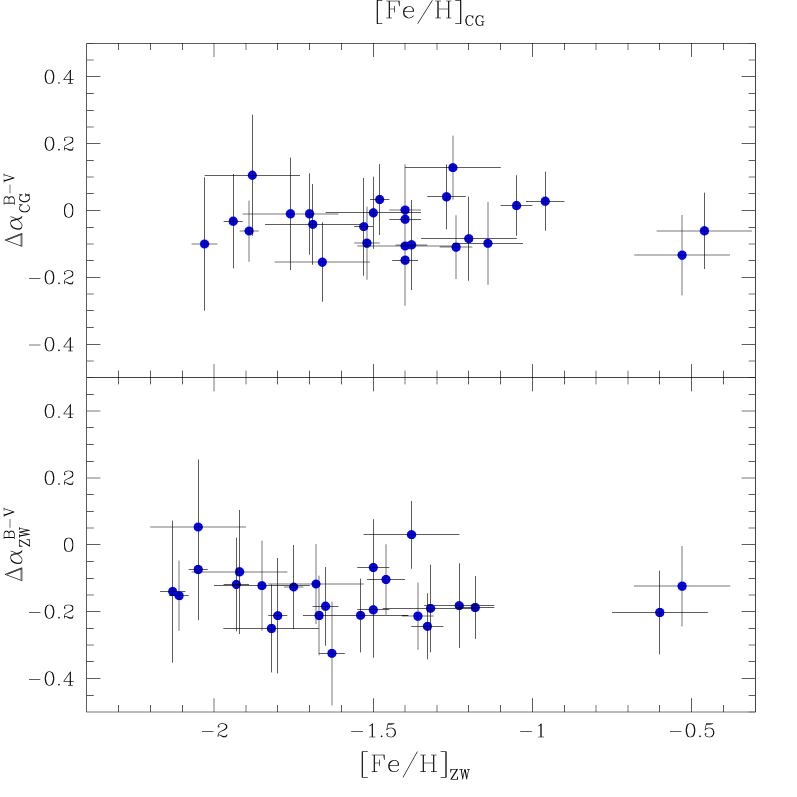
Figure 16: The estimated $\Delta\alpha$ differences for each object observed in $B-V$, and the reference G00 isochrone of age 14 Gyr, as a function of metallicity in the ZW (bottom panel) and CG97 scales (upper panel). Notice the absence of any significant trend with metallicity.

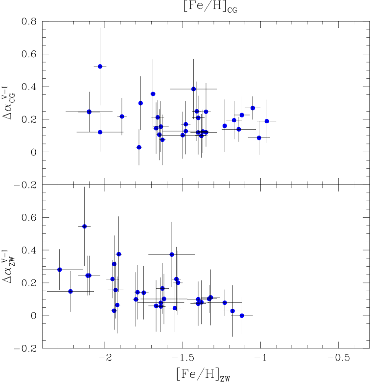
Figure 17: The same as in Fig. 16, but for the clusters observed in $V-I$.

We have then modeled the data in Figs. 16 and 17 by least-squares fitting of either (i) a constant value, or (ii) a straight line. The results are presented in Table 3.

Table 3: Fitting parameters for the data in Figs. 16 and 17.

(i) A constant value: $\Delta\alpha=a$
Case	$a$	$\sigma_{a}$			$\chi^{2}$
CG scale, $BV$ data	$-$0.036	0.022			10.28
ZW scale, $BV$ data	$-$0.157	0.025			9.82
CG scale, $VI$ data	0.178	0.022			13.11
ZW scale, $VI$ data	0.133	0.024			15.59
(i) A straight line: $\Delta\alpha=a+b\,({\rm[Fe/H]}+1.5)$
Case	$a$	$\sigma_{a}$	$b$	$\sigma_{b}$	$\chi^{2}$
CG scale, $BV$ data	$-$0.036	0.023	$-$0.009	0.059	10.26
ZW scale, $BV$ data	$-$0.157	0.025	$-$0.027	0.064	9.64
CG scale, $VI$ data	0.174	0.024	$-$0.028	0.066	12.92
ZW scale, $VI$ data	0.108	0.026	$-$0.173	0.071	9.71

In the case of $BV$ data, the fitted lines turned out to have a negligible slope, and there is virtually no improvement in the fittings as we pass from a constant to a straight line. The same applies for the $VI$ data in the CG97 scale. The case of $VI$ data on the ZW scale, with its mild slope ($-0.17\pm 0.07$), constitutes the only exception.

Perhaps more importantly is the fact that, assuming that $\alpha$ is constant (first part of Table 3), we get extremely small values for its dispersion, i.e. $\sigma_{\alpha}\simeq 0.023$. This has to be compared to typical values of $\alpha$ assumed in evolutionary calculations, i.e. $\alpha\sim 1.7$. Overall, these numbers indicate that, indeed, the empirical data can be very well approximated by a constant value of $\alpha$.

6 A new metallicity index?

We have shown that there is a relation between $W_{\rm HB}$ and the metal content of the cluster. Since $W_{\rm HB}$ has only a second order dependence on the reddening (which can be corrected as described in Appendix), it is a potentially interesting metallicity index. We have verified whether it is possible to use this parameter as a new metallicity index. In Fig. 18 we fitted a parabola to the observed $W_{\rm HB}^{(B-V)}$ vs [Fe/H] relation for the hst sample, obtaining a $0.1$ dex rms residual.

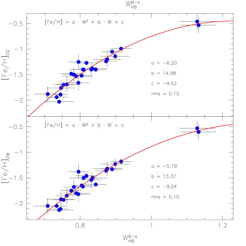
Figure 18: Calibration of $W_{\rm HB}^{B-V}$ as a metallicity index. The observed data points have been interpolated with a second order polynomial.

The sensitivity of the parameter, although lower than that of other traditional indices, can be used to obtain a first estimate of the metallicity. A typical $0.04$ magnitude error on $W^{B-V}_{\rm HB}$ would translate into a $\sim 0.2$ dex uncertainty on [Fe/H]. On the other hand, the lack of metal-rich clusters, and the much shallower dependence on metallicity of this parameter, prevents a reliable calibration of $W^{V-I}_{\rm HB}$.

There could be some concern about the inclusion of the two metal-rich clusters (NGC 6388 and NGC 6441) in the $B-V$ calibration, since it is still not known what drives the peculiar morphology of the HB of these two objects. Therefore, we have also calibrated the $W^{B-V}_{\rm HB}$ index in the $-2.1<$[Fe/H]$<-1.0$ metallicity interval. In this case we used the weighted linear least squares fit, which is shown in Figs. 19 and 20. The result of the fits shows that the relation for $W^{B-V}_{\rm HB}$ has still a formally low dispersion ($0.1$ dex rms), whereas a large $0.3$ dex dispersion is shown by the residuals for the $W^{V-I}_{\rm HB}$ parameter. Again, this confirms the higher sensitivity of $W^{B-V}_{\rm HB}$ to metallicity changes.

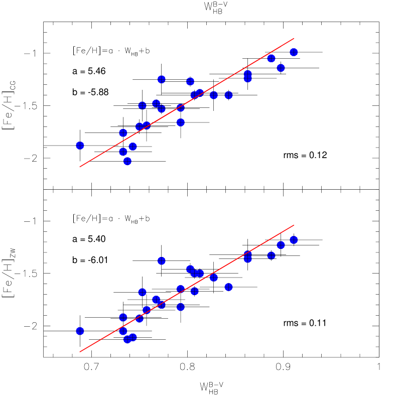
Figure 19: Calibration of $W^{B-V}_{\rm HB}$ for the hst clusters, obtained with the exclusion of NGC 6388 and NGC 6441. The parameters of the weighted least square interpolation are reported in the figures, both for the CG97 (upper panel) and ZW84 (lower panel) metallicity scales.

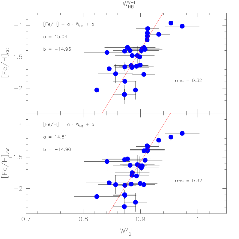
Figure 20: Same as Fig. 19, for the ground-based data.

In Fig. 21, which shows the trend of the second order reddening corrections that must be applied to $W_{\rm HB}$, the right vertical axis shows how a difference in $W_{\rm HB}$ translates into a difference in metallicity, using the above relations. It clearly shows that, especially for the highly reddened clusters, neglecting the differential reddening corrections would lead to significant systematic errors in the estimated metallicity. For instance, the error on [Fe/H] for NGC 6287 would be of the order of $0.2$ dex. Naturally, these errors are larger for metallicities obtained using the $V-I$ calibration.

In any case, we must note that: (i) The rms error are just formal fitting errors, while the real uncertainty on the metallicity is higher, as it must take into account the error on the metal content of the calibrating clusters and the photometric calibration errors; (ii) The relations obtained in this paragraph can be used only in a limited metal interval and for a limited sample of clusters, which must have a blue HB.

7 Summary and discussion

In this paper, we took advantage of the homogeneous photometric databases of Galactic globular clusters, presented in Rosenberg et al (2000a , 2000b ) and Piotto et al. (piottoEtal02 (2002)), to complete another step in the characterization of the morphological properties of the CMD of GGCs, and in the fine-tuning of the theoretical models. To this aim, the $W_{\rm HB}$ parameter, originally defined in B98, has been measured for all suitable clusters, and appropriate corrections to account for differential reddening effects have been applied. The quality of the new data sets has allowed to settle the original question posed in B98. The trend of $W_{\rm HB}$ with metallicity showed a dispersion that was larger than formal measurement errors, a fact that can now be attributed to the inhomogeneous data sources employed.

The dispersion of $W_{\rm HB}$ around the mean trend with metallicity, is now compatible with the error bar on the data points. This means that (a) one can reverse the argument and use $W_{\rm HB}$ to have a first-order guess on a cluster metallicity (Sect. 6), and (b) that whatever other variables influence the parameter, they must have a well-defined dependence on [Fe/H] (including zero dependence).

The second point was investigated in some detail by comparing the data to two independent sets of theoretical calculations. First, it was noted that the observed trend of $W_{\rm HB}$ with metallicity (which is stronger for the $B-V$ color) is well reproduced by both isochrone sets, although a zero-point problem in the $(V-I)$ color-temperature transformations seems to be present.

In order to test the dependence on all other variables influencing $W_{\rm HB}$, their values were varied within reasonable limits. For any variable $x$, we checked the $W_{\rm HB}$ vs. $x$ trend at several fixed metallicities, and noticed that these trends can be well approximated with linear relations. This means that we could use the slope $\Delta W_{\rm HB}/\Delta x$ to rank the relative dependencies. We concluded that the influence of the helium content is negligible, and that that of the mixing-length parameter $\alpha$ is much stronger than that of the age (see Table 2). This fact was then exploited to investigate a long-standing theoretical problem of stellar evolution, whether $\alpha$ should be varied with metallicity or not. From our comparisons, we find no trend of $\alpha$ with the metal content of a cluster.

With respect to the color-$T_{\rm eff}$ transformations, a test was made by adopting either the Alonso et al. (alonsoEtal99 (1999)) or the Kurucz (kurukz92 (1992)) relations. This showed that, potentially, the $B-V$ transformations could make a much larger difference than the $V-I$ transformations. However, since actually the theoretical $V-I$ colors show the greater problems, the agreement between the two transformations implies that a deep revision for them is needed.

Finally, we examined the question of whether models with enhanced $\alpha$-elements better reproduce the CMD morphology of GGCs. The conclusion is that, unfortunately, the existence of two discrepant metallicity scales leaves this question open. The best results are obtained in the $\alpha$-enhancement scenario, and adopting the ZW84 metallicity scale. However, one could well adopt the CG97 scale and claim that the $B-V$ color-transformations are wrong, since we have seen how much they change from author to author. Thus, we must conclude that there is an urgent need for an independent metallicity scale (which also involves the question of galactic chemical evolution models, see Saviane & Rosenberg sr99 (1999)).

Appendix A Differential reddening corrections

A.1 Corrections according to Olson

Olson (Olso75 (1975)) obtained the following relation:

$$R=3.25+0.25\times(B-V)_{0}+0.05\times E_{B-V}$$

¿From the definition of $R=\left({\frac{A_{V}}{E_{B-V}}}\right)$ and of the color excess, we can write:

$$W^{0}_{\rm HB}=(B-V)^{0}_{\rm RGB}-(B-V)_{\rm TD}^{0} =$$

$$=(B-V)_{\rm RGB}-E^{\rm RGB}_{B-V}-(B-V)_{\rm TD}+E^{\rm TD}_{B-V} =$$

$$=W_{\rm obs}+(E^{\rm TD}_{B-V}-E^{\rm RGB}_{B-V}) =$$

$$=W_{\rm obs}+\left(\left.\frac{A_{V}}{R}\right|_{\rm TD}-\left.\frac{A_{V}}{R}\right|_{\rm RGB}\right)$$

Since $A_{V}$ is little dependent on the color, we substitute an average value in the equation, $\left<{A_{V}}\right>$, obtaining:

$$W_{\rm HB}^{0}=W_{\rm obs}+\left<{A_{V}}\right>\left({\frac{R^{RGB}-R^{TD}}{R^{TD}\cdot{R^{RGB}}}}\right).$$

Now we substitute the product of $R^{\rm TD}$ times $R^{\rm RGB}$ by $R^{2}$, and using Olson expression, we find:

$$W^{0}_{\rm HB}=$$

$$=W_{\rm obs}+<A_{V}>\left\{\frac{0.25\,[(B-V)^{\rm RGB}_{0}-(B-V)^{\rm TD}_{0}]}{R^{2}}\right\}=$$

$$=W_{\rm obs}+\frac{0.25\,E_{B-V}\,\Delta(B-V)_{0}}{R}$$

Here ${\textrm{E}_{B-V}}\left(=\frac{\left<A_{V}\right>}{R}\right)$ is the average color excess of the single cluster, taken from Harris (harris96 (1996)), and we assumed $R=3.1$. As a typical value of ${\Delta(\textrm{B}-\textrm{V})_{0}}$ we used $0.8$ magnitudes, which is the $W^{B-V}_{\rm HB}$ value of NGC 1904, taken from B98 who applied the same differential reddening correction. In conclusion, the observed values of $W^{B-V}_{\rm HB}$ must be corrected with the expression:

$$W^{0}_{\rm HB}=W_{\rm obs}+0.064\times E_{B-V}$$ (1)

A.2 Corrections according to Grebel and Roberts

Grebel and Roberts (greb95 (1995); GR95) provide tables that give color excesses, absorptions, and the $R$ ratio for different photospheric temperatures, gravities and metallicities (${[\textrm{Fe}/\textrm{H}]}=0.0,\,-1.0,\,-2.0$). Since we are applying a second-order correction, we used the tables relative to the intermediate metallicity.

We start again from the relation

$$W^{0}_{\rm HB}=W_{\rm obs}=(E^{\rm TD}_{B-V}-E^{\rm RGB}_{B-V})$$ (2)

And we find the color excesses using the relation

$$R=\frac{A^{\rm tab}_{V}}{E^{\rm tab}_{B-V}}=\frac{<A_{V}>}{E^{\rm col}_{B-V}}$$ (3)

where $A_{V}^{\rm tab}$ and ${\textrm{E}_{B-V}^{\rm tab}}$ are the tabular values from GR95, ${\textrm{E}_{B-V}^{\rm col}}$ is the color excess for a given cluster and given color (to be determined), and $\left<{A_{V}}\right>$ is an average value of the total absorption, which can be calculated with the expression:

$$<A_{V}>=3.1\times E^{\rm cat}_{B-V}$$

where ${\textrm{E}_{B-V}^{cat}}$ is the mean reddening taken from Harris (harris96 (1996)).

Equation (3) is justified by the fact that the ratio of total to selective absorption is constant. Thus, it can be used to find ${\textrm{E}_{B-V}}$ for any TD and RGB color, since:

$$E^{\rm col}_{B-V}=3.1\frac{E^{\rm cat}_{B-V}}{R}$$ (4)

We now insert Eq. (4) into Eq. (2), and taking $R$ from GR95 tables, we obtain

$$W^{0}_{\rm HB}=W_{\rm obs}+3.1\times\left(\frac{1}{R_{\rm TD}}-\frac{1}{R_{\rm RGB}}\right)\times E^{\rm cat}_{B-V} =$$

$$=W_{\rm obs}+c\times E^{\rm cat}_{B-V}$$ (5)

This last equation (5) is formally similar to Eq. (1), but in this case $c$ is a variable that depends on the color of the two CMD points. The variations of $c$ are, as expected, of the order of a thousandth of a magnitude.

A.3 Corrections to the ${(\textrm{V}-\textrm{I})}$ measurements

The analogous of Eq. (2) is the following

$$W^{0}_{\rm HB}=W_{\rm obs}+(E^{\rm TD}_{V-I}-E^{\rm RGB}_{V-I})$$ (6)

The ${\textrm{E}_{V-I}}$ values can be computed from ${\textrm{E}_{B-V}}$

$$E^{\rm col}_{V-I}=\left(\frac{E_{V-I}}{E_{B-V}}\right)^{\rm tab}\times E^{\rm col}_{B-V}$$ (7)

where, like before, “tab” quantities depend on the temperature and are taken from GR95 tables, while “col” quantities are referred to different zones of each cluster’s CMD. Thus ${\textrm{E}_{B-V}^{\rm col}}$ is the value of the blue color excess (Eq. 4), while ${\textrm{E}_{V-I}^{\rm col}}$ is the value of the color excess that must be computed.

Substituting Eq. (7) into Eq. (6), and using Eq. (4), one obtains:

$$W^{0}_{\rm HB}=$$

$$=W_{\rm obs}+\left[\left(\frac{E_{V-I}}{E_{B-V}}\right)^{\rm tab}_{\rm TD}E^{\rm TD}_{B-V}-\left(\frac{E_{V-I}}{E_{B-V}}\right)^{\rm tab}_{\rm RGB}E^{\rm RGB}_{B-V}\right]=$$

$$=W_{\rm obs}+3.1\left[\left(\frac{1}{R}\frac{E_{V-I}}{E_{B-V}}\right)^{\rm tab}_{\rm TD}-\left(\frac{1}{R}\frac{E_{V-I}}{E_{B-V}}\right)^{\rm tab}_{\rm RGB}\right]E^{\rm cat}_{B-V}=$$

$$=W_{\rm obs}+c^{\prime}\cdot E^{\rm cat}_{B-V}$$

The corrections to the two $W_{\rm HB}$ are plotted in Fig. 21 as a function of $E_{B-V}$. It is then clear that $(V-I)$ colors are $\sim 2$ times less sensitive to this effect.

Figure 21: The corrections that must be applied to $W_{\rm HB}$ are plotted versus the selective absorption $E_{B-V}$. Values relative to $(B-V)$ color differences are displayed in the lower panel, while the upper panel displays the corrections to $(V-I)$ color differences. The right vertical axis shows the impact on [Fe/H] values if inferred from $W_{\rm HB}$ (see Sect. 6).

References

- (1) Alexander, D. R., & Ferguson, J.W. 1994, ApJ, 437, 879
- (2) Alonso, A., Arribas, S., & Martínez-Roger, C., 1999, A&AS 140, 261
- (3) Alonso, A., Salaris, M., Arribas, S., Martínez-Roger, C., & Asensio Ramos, A. 2000, A&A, 355, 1060
- (4) Bedin, L. R., et al. 2000, A&A, 363, 159
- (5) Bertelli, G., Bressan, A., Chiosi, C., Fagotto, F., & Nasi, E. 1994, A&AS, 106, 275
- (6) Böhm-Vitense, E. 1958, Z. Astroph., 46, 108
- (7) Bono, G., Cassisi, S., Zoccali, M., & Piotto, G., 2001, ApJ 546, L109
- (8) Brocato, E., et al. 1998, A&A, 335, 929 (B98)
- (9) Canuto, V. M., & Mazzitelli, I. 1991, ApJ, 370, 295
- (10) Carretta, E., & Gratton, R. 1997, A&AS, 121, 95 (CG97)
- (11) Cassisi, S., Castellani, V., Degl’Innocenti, S., Salaris, M., & Weiss, A. 1999, A&AS, 134, 103
- (12) Castellani, V., Degl’Innocenti, S., & Marconi, M. 1999, MNRAS, 303, 265
- (13) Castellani, V., et al. 2000, A&A, 354, 150
- (14) Castelli, F., Gratton, R. G., & Kurucz, R. L. 1997, A&A, 318, 841
- (15) Girardi, L., Bressan, A., Bertelli, G., & Chiosi, C. 2000, A&AS, 141, 371 (G00)
- (16) Gratton, R. G., Carretta, E., & Castelli, F. 1996, A&A, 314, 191
- (17) Grebel, E., & Roberts, W. 1995, A&AS, 109, 293 (GR95)
- (18) Harris, W. E. 1996, AJ, 112, 1487
- (19) Iglesias, C. A., & Rogers, F. J. 1993, ApJ, 412, 752
- (20) Kurucz, R., 1992. In The Stellar Populations of Galaxies, IAU Symp. 149, ed. Beatriz Barbuy and Alvio Renzini. Kluwer: Dordrecht, p. 225
- (21) Ludwig, H.-G., Freytag, B., & Steffen, M. 1999, A&A, 346, 111
- (22) Olson, B. 1975, PASP, 87, 349
- (23) Piotto, G., Rosenberg, A., Saviane, I., Aparicio, A., & Zoccali, M. 2000, in The Galactic Halo: From Globular Cluster to Field Stars, Proceedings of the 35th Liege International Astrophysics Colloquium. Eds. A. Noels et al., Liege, Belgium: Institut d’Astrophysique et de Geophysique, p.471
- (24) Piotto, G., et al., 2002, A&A accepted
- (25) Renzini, A., & Fusi Pecci, F. 1988, ARA&A, 26, 199
- (26) Rogers, F. J., & Iglesias, C. A. 1992, ApJS, 79, 507
- (27) Rosenberg, A., Saviane, I., Piotto, G., & Aparicio, A. 1999, AJ, 118, 2306
- (28) Rosenberg, A., Piotto, G., Saviane, I., & Aparicio, A. 2000a, A&AS, 144, 5
- (29) Rosenberg, A., Aparicio, A., Saviane, I., & Piotto, G. 2000b, A&AS, 145, 451
- (30) Rutledge, A. G., Hesser, J. E., & Stetson, P. B. 1997, PASP, 109, 907 (RHS97)
- (31) Salaris, M., Chieffi, A., & Straniero, O., 1996, ApJ 414, 580
- (32) Salaris, & Weiss A., 1998, A&A 335, 943
- (33) Salasnich, B., 2001, PhD thesis, Università di Padova, Italy
- (34) Salasnich, B., Girardi, L., Weiss, A., & Chiosi, C., 2000, A&A 361, 1023
- (35) Saviane, I., & Rosenberg, A. 1999, The Analytic Way to the Red Giant Branch, in Liège Int. Astroph. Coll. July 5-8, 1999
- (36) Spruit, H. C. 1997, Mem. Soc. Astron. It., 68, 397
- (37) Weiss, A., & Salaris, M. 1999, A&A, 346, 897
- (38) Weiss, A., & Schlattl, H. 1998, A&A, 332, 215
- (39) VandenBerg, D. A., Swenson, F. J., Rogers, F. J., Iglesias, C. A., & Alexander, D. R. 2000, ApJ, 532, 430 (V00)
- (40) Zinn, R., & West, M. J. 1984, ApJS, 55, 45 (ZW84)
- (41) Zoccali, M., et al. 2000, ApJ 538, 289