Non–linear magnetic field decay in neutron stars –
Theory and observations

There exists both theoretical and observational evidence that the magnetic field decay in neutron stars may proceed in a pronounced non–linear way during a certain episode of the neutron star’s life. In the presence of a strong magnetic field the Hall–drift dominates the field evolution in the crust and/or the superfluid core of neutron stars. Analysing observations of $P$ and $\dot{P}$ for sufficiently old isolated pulsars we gain strong hints for a significantly non–linear magnetic field decay. Under certain conditions with respect to the geometry and strength of a large–scale magnetic background field an instability is shown to occur which rapidly raises small–scale magnetic field modes. Their growth rates increase with the background field strength and may reach $\sim 10^{4}$ times the ohmic decay rate. Consequences for the rotational and thermal evolution as well as for the cracking of the crust of neutron stars are discussed.

1 Introduction

There is still an ongoing scientific debate whether the magnetic fields of pulsars decay at all (see, e.g., Regimbau & de Freitas Pacheco 2001, and references therein). Thus, the question whether this questionable decay proceeds in a non–linear way seems to be somewhat academic. However, the neutron star magnetic fields are the strongest known in the universe and already this very fact suggests the idea that, if there is a field evolution at all, it should be a non–linear one. As we will show, there exist both theoretical and observational evidences that the field decay proceeds essentially in a non–linear way, at least in certain regions of the star and surely only during certain episodes of its life.

In order to be able to deal with well defined physical conditions we confine ourselves here to considering the evolution of sufficiently old isolated neutron stars (SOINSs). We characterize them by the following properties:

• the supernova fall–back accretion phase is finished and a stable density stratification $\rho(r)$ has been established;

• the rediffusion of the magnetic field has been completed;

• the rotation is slow enough so that the irradiation of gravitational waves does not contribute to the spin down;

• the appearance of glitches is less probable;

• the crust is almost completely crystallized;

• the temperature profile has become flat enough, to avert convection in the outermost thin liquid layer and in the core region as well as the occurrence of a thermoelectric instability in the crust;

• the electron relaxation time is already so large that the magnetization parameter may reach values large enough to make the electron transport processes non–linear;

• the absence of accretion, as a consequence of isolation, ensures that there are neither external sources of angular momentum nor of heating;

• therefore, there is a stable compactness ratio $M/R$ and no screening of the magnetic field can happen.

All these constraints are met by the majority of neutron stars the age of which is $\gtrsim 10^{5}$ years. Therefore, if any thermal and/or rotational evolution of SOINSs is observed beyond that predicted when assuming a constant magnetic field, it is with a high probability caused by an evolving one.

Here, we intend to consider as the non–linearity of the field evolution the Hall–effect or Hall–drift, as it occurs in the crust (see, e.g., Shalybkov & Urpin 1997), i.e., both ambipolar diffusion and any convective motion of the neutron star matter is excluded.
The effect of the Hall–drift on the magnetic field evolution of isolated neutron stars has been considered by a number of authors (see, e.g., Haensel et al. 1990; Goldreich & Reisenegger 1992; Muslimov 1994; Naito & Kojima 1994; Shalybkov & Urpin 1995, 1997; Urpin & Shalybkov 1995, 1999; Vainshtein et al. 2000). They discussed the redistribution of magnetic energy from an initially large–scale (e.g., dipolar) field into small–scale components via the Hall–term. Though the Hall–drift itself is a non–dissipative process, these changes in the field geometry may in principle accelerate the field decay. However, the results presented in Naito & Kojima (1994), Muslimov (1994), Shalybkov & Urpin (1997), and Urpin & Shalybkov (1999) suggest the conclusion that the field decay is not modified drastically.

Goldreich & Reisenegger Goldreich & Reisenegger (1992) developed the idea of the Hall–cascade, i.e., when starting with a large–scale magnetic field small–scale field components are generated down to a scalelength $l_{\text{crit}}$, where the ohmic dissipation begins to dominate the Hall–drift.

In some of the above–mentioned investigations numerical instabilities are mentioned if either the field structure becomes too complex (Urpin & Shalybkov 1995) or the initial field is too strong (Naito & Kojima 1994; Urpin & Shalybkov 1999). Also, when considering the thermomagnetic field generation in the crust of young neutron stars (Wiebicke & Geppert 1996), where small–scale modes are the first ones to be excited, numerical instabilities occurred exclusively caused by the Hall–drift.

Recently we have shown (Rheinhardt & Geppert 2002) that all the observed instabilities are in their essence very likely not of numerical origin but have physical reasons: A sufficiently strong and inhomogeneous large–scale background field is unstable with respect to small–scale perturbations, which rise very rapidly in comparison with the relevant ohmic decay time of the background field. This rapid transfer of energy from the background into small–scale field components proceeds not via a cascade but jump–like across wide spectral distances. The unstable perturbations show small radial structures close to the neutron star’s surface whereas their lateral structures are of medium size. Of course, this Hall–instability can act only during an episode of the field decay, which unavoidably leads to a zero field. This episode, however, may have observable consequences.

In the following we will present the theoretical and observational hints for the non–linear field decay in isolated neutron stars. After a description of the Hall–drift induced field instability we discuss its effects on observable quantities of the above introduced SOINSs.

2 Theoretical motivation

Under which conditions becomes the evolution of the magnetic field non–linear? The field evolution is determined by Maxwell’s equations in quasi–stationary approximation

$$\dot{\@vec{B}}=-c\,\operatorname{curl}\@vec{E}\;,\quad\operatorname{div}\@vec{B}=0\;,\quad\@vec{j}=\frac{c}{4\pi}\operatorname{curl}{\@vec{B}}$$ (1)

together with Ohm’s law, which has in the absence of convective motions the form

$$\@vec{E}=\hat{\sigma}^{-1}\@vec{j}=\hat{R}\@vec{j}\leavevmode\nobreak\ \leavevmode\nobreak\ .$$ (2)

In the presence of a magnetic field the electric conductivity, $\hat{\sigma}$, and the resistivity, $\hat{R}$, respectively, become tensors whose components parallel and perpendicular to the magnetic field along with their Hall–component are represented by

$$\hat{\sigma}=\left(\begin{array}[]{lll}\phantom{-}\sigma_{\perp}&\sigma_{\text{H}}&0\\ -\sigma_{\text{H}}&\sigma_{\perp}&0\\ \phantom{-}0&0&\sigma_{\parallel}\end{array}\right)=\hat{R}^{-1}=\left(\begin{array}[]{lll}\phantom{-}R_{\perp}&R_{\text{H}}&0\\ -R_{\text{H}}&R_{\perp}&0\\ \phantom{-}0&0&R_{\parallel}\end{array}\right)^{-1}\!\!\!\!\!\!,$$ (3)

if $\@vec{B}$ goes along the $\@vec{z}$–axis.

Let us consider the evolution of a magnetic field completely confined in the crust of the neutron star. There, the field could have been generated either by convection in the outermost layers of the proto–neutron star or by a thermoelectric instability during the early period of the neutron star’s life, when the temperature gradient in the liquid crust is extremely large (see, e.g., Urpin et al. 1986; Wiebicke & Geppert 1996). A peculiarity of the transport processes in the crust is that the components of the resistivity tensor parallel and perpendicular to the magnetic field coincide (see Yakovlev & Shalybkov 1991), because the electrons move as a degenerate gas through the crystal lattice of the crust. In relaxation time approximation they found

$$\sigma_{\parallel}=\sigma_{0}\,,\quad\sigma_{\perp}=\frac{\sigma_{0}}{1+(\omega_{B}\tau)^{2}}\,,\quad\sigma_{\text{H}}=\omega_{B}\tau\,\sigma_{\perp},$$ (4)

where $\omega_{B}=eB/m_{e}^{\ast}c$ is the Larmor frequency of the electrons, $m_{e}^{\ast}$ their effective mass, and $\tau$ their relaxation time between two collisions with the phonons or impurities of the crustal lattice. As a consequence of Eq. (4) the parallel and perpendicular components of the resistivity tensor just coincide

$$R_{\parallel}=R_{\perp}=\frac{\sigma_{\perp}}{\sigma_{\perp}^{2}+\sigma_{\text{H}}^{2}}=\sigma_{0}^{-1}\,,\quad R_{\text{H}}=\frac{\sigma_{\text{H}}}{\sigma_{\perp}^{2}+\sigma_{\text{H}}^{2}}.$$ (5)

The scalar electric conductivity $\sigma_{0}$ as well as the relaxation time $\tau$ are complicated functions of the density $\rho(r)$, the temperature $T(r,t)$, the impurity concentration $Q$ and of the chemical composition (i.e., charge number $Z(r)$ and mass number $A(r)$; see, e.g., Urpin & Yakovlev 1980).

Ohm’s law (2) together with Eq. (3) allows of representing the electric field by use of the unit vector of the magnetic field $\@vec{e}_{B}=\@vec{B}/|\@vec{B}|$ as

$$\@vec{E}=R_{\parallel}(\@vec{e}_{B}\cdot\@vec{j})\@vec{e}_{B}+R_{\perp}(\@vec{e}_{B}\times\@vec{j})\times\@vec{e}_{B}+R_{\text{H}}(\@vec{j}\times\@vec{e}_{B}),$$ (6)

which because of $R_{\perp}=R_{\parallel}$ yields

$$\@vec{E}=R_{\parallel}\@vec{j}+R_{\text{H}}(\@vec{j}\times\@vec{e}_{B})=\sigma_{0}^{-1}\big{(}\@vec{j}+\omega_{B}\tau(\@vec{j}\times\@vec{e}_{B})\big{)}.$$ (7)

Taking now the $\operatorname{curl}$ of $\@vec{E}$ and using Ampere’s law we arrive at the Hall–induction equation for the crystallized neutron star crust:

$$\dot{\@vec{B}}=-\frac{c^{2}}{4\pi}\operatorname{curl}\bigg{(}\frac{1}{\sigma_{0}}\big{(}\operatorname{curl}\@vec{B}+\omega_{B}\tau\,(\,\operatorname{curl}\@vec{B}\;\leavevmode\nobreak\ \leavevmode\nobreak\ \times\@vec{e}_{B}\,)\big{)}\!\bigg{)}$$ (8)

which makes immediately clear that the field decay will proceed in a significantly non–linear manner as soon as (and where)

$$\frac{eB(r,t)}{m_{e}^{\ast}(r)c}\tau\big{(}\rho(r),T(r,t),Q,A(r),Z(r)\big{)}>1\;,$$ (9)

i.e., the significance of the non–linearity depends not only on the field but on all the complex physical conditions in the crust.

In order to get an impression how the magnetization parameter $\omega_{B}\tau$ in the crust of an isolated neutron star evolves we present here results obtained by Page et al. (2000) for a neutron star whose state of matter in the core is described by a medium equation of state. The initial polar surface field strength is assumed to be $10^{13}$ G, the density up to which the field is initially penetrating is $\rho_{0}=10^{14}$g cm^-3; for the impurity concentration $Q=0.01$ is supposed and the chemical composition of the crust should be that of cold catalyzed matter.

Figure 1: The magnetization parameter $\omega_{B}\tau$ as a function of the density at different moments of neutron star’s life.

Since the field decay as presented by Page et al. (2000) has been calculated just by neglecting the non–linear effects, i.e., considering only the linear ohmic decay, Fig. 1 does not present the “real” evolution of $\omega_{B}\tau$ because $\@vec{B}(r,t)$ certainly evolves differently under the influence of a strong Hall–drift. Nevertheless, these results may serve as a strong hint that the latter may play an important role for the magnetic field decay in neutron stars. When, e.g., $\omega_{B}\tau$ becomes as large as $1000$ as a consequence of the star’s cooling down due to which the electron relaxation time rises by orders of magnitude, a linear description of the field decay is surely no longer justified.

3 Observational motivation

The best known observational quantities of SOINSs are obtained when they appear as radiopulsars: their pulsation period $P=2\pi/\Omega$ ($\Omega$ being the related rotational velocity), its time derivative $\dot{P}$ and, unfortunately only in a few cases, its second time derivative $\ddot{P}$. The spin–down behaviour is to a high accuracy determined by the requirement, that the loss of rotational energy ${E}_{\text{rot}}=I\Omega^{2}/2$ ($I$ is the moment of inertia of the neutron star) is equal to the power of the magneto–multipole radiation $\dot{E}_{\text{mmr}}$, emitted by the rotating magnetized neutron star appearing as a radio pulsar:

$$\dot{E}_{\text{rot}}=I\Omega\dot{\Omega}\approx-\dot{E}_{\text{mmr}}.$$ (10)

As already discussed above, for pulsars older than $\approx 10^{5}$ years, the spin–down as a consequence of the emission of gravitational waves can surely be neglected, too. The loss of angular momentum due to a relativistic wind of charged particles (caused by the pulsar mechanism) shows the same functional dependences on the neutron star radius $R$, the magnetic field and the rotational velocity as the magneto–multipole radiation (Shapiro & Teukolsky 1983). Clearly, Eq. (10) is not valid during glitches.

According to Krolik (1991) the power of the magneto–multipole radiation is given by

$$\dot{E}_{\text{mmr}}=\frac{c}{8\pi}\sum_{l,m}S_{lm}^{-2}\left[\frac{2^{l}l!}{(2l)!}\right]^{2}\!\!\left(\frac{mR\Omega}{c}\right)^{2(l+1)}\!\!R^{2}\langle|\@vec{B}_{lm}|\rangle^{2},$$ (11)

where $\langle|\@vec{B}_{lm}|\rangle$ is the average of the multipole component of the magnetic field, defined by its multipolarity $l$ and projection $m$, across the spherical surface. $S_{lm}$ is a constant reflecting the geometry of $\@vec{B}_{lm}$ (see Krolik, Krolik 1991). Since $R$ and $I$ are fixed for SOINSs, we have with Eqs. 10 and (11) an unambiguous relation between the observational quantities $P$ and $\dot{P}$ and the magnetic field. In other words, if we were able to calculate all the multipole components of the magnetic field as functions of time and if these together with the measured quantities $P(t)$ and $\dot{P}(t)$ satisfied Eq. (10), we had understood the field decay. However, as a consequence of the sum occurring in Eq. (11) it is impossible to infer from $P(t)$ and $\dot{P}(t)$ all the $\langle|\@vec{B}_{lm}|\rangle$ in an unambiguous way. Therefore, we consider here only one term of the sum to be responsible for the spin–down and denote the corresponding $\langle|\@vec{B}_{lm}|\rangle$ simply by $B$. (Usually, the dipolar term, $l=m=1$, is chosen.) Then, by equating Eq. (10) with Eq. (11), the change of the neutron star’s rotation can be written as

$$\dot{\Omega}=-K\Omega^{n}$$ (12)

where the constant $K$ comprises the geometrical constant $S_{lm}$ as well as radius and moment of inertia and the magnetic field. The exponent $n=2l+1$ is called the “braking index”, where $n=3$ for a pure rotating dipole. The standard way to calculate the braking index is to take the time derivative of Eq. (12) resulting in

$$n=\frac{\ddot{\Omega}\Omega}{\dot{\Omega}^{2}}=2-\frac{\ddot{P}P}{\dot{P}^{2}}\;.$$ (13)

However, $\ddot{\Omega}$ (or $\ddot{P}$) can be obtained with sufficient accuracy for a few young pulsars only.

Johnston & Galloway (1999) suggested an alternative way to calculate $n$ without employing $\ddot{P}$. By direct integration of Eq. (12) over a time interval $T\gg P$

$$\int_{\Omega_{1}}^{\Omega_{2}}\frac{\text{d}\Omega}{\Omega^{n}}=-KT$$ (14)

they calculate the braking index by

$$n=1+\frac{\Omega_{1}\dot{\Omega}_{2}-\Omega_{2}\dot{\Omega}_{1}}{\dot{\Omega}_{1}\dot{\Omega}_{2}T}\,,$$ (15)

i.e., knowing the rotational period and its time derivative of two observations, separated by $T$, one is able to obtain the braking index without needing $\ddot{P}$. For the Crab pulsar and B 1509–58 they found a good coincidence of the values of $n$ obtained with both methods. Thus, there exists a certain warranty that the application to other radio pulsars will yield reliable results, too. In their Table 1 Johnston & Galloway (1999) present the braking index $n$, calculated according to Eq. (15) along with $P$ and $\dot{P}$ for 20 pulsars. Six of them have negative braking indices which possibly could be understood as due to the occurrence of glitches or the continuation of a post–glitch recovery during the observational periods. As will become clear later, a decay of the NS magnetic field can never be responsible for these negative values (whereas a field growth can). The eight pulsars with the smallest error bars for $n$ (B0540+23, B0611+22, B0656+14, B0740–28, B1915+13, B2002+31, B2148+52 and B2334+61) have all positive braking indices, five of them with $n>20$. Because of their similar braking indices B0919+06, B1221-63 and B1907+10 may belong to that group too, but their error bars are much larger. Two further pulsars, B0154+61 and B1356-60, with $n>3$ have unacceptably large error bars. By use of a recently available pulsar catalogue (Manchester et al. 2001) we found two more SOINSs (B0727-18, B1822-09) for which also earlier observations exist (Taylor et al. 1993). Their derived values of $n$ are the largest found by the above method, although the error of $n$ for B1822-09 is rather high (about 60%). All pulsars mentioned have an active age $\tau_{a}=P/2\dot{P}$ between $4.13\cdot 10^{4}$(B2334+61) and $1.7\cdot 10^{6}$ (B1907+10) years, i.e., are just at the range of ages, the SOINSs should be. For a collection of the selected SOINSs’ data see Table 1.

A basic supposition for both methods to calculate the braking index is that the coefficient $K$ in Eq. (12), by virtue of Eq. (11) proportional to $B^{2}$, is really a constant. Now let us relax that assumption in so far as we will allow for a varying field while the other quantities entering $K$ remain constant, in agreement with our concept of SOINSs. Then we can rewrite Eq. (12) into

$$\dot{P}={\cal{K}}B^{2}(t)P^{-n+2}\,,$$ (16)

where for a standard neutron star ($R=10^{6}$cm, $I=10^{45}$gcm²) the constant ${\cal{K}}\approx 10^{-39}$ cm s³g^-1 if $n=3$. We will nevertheless assume in the following that the rotational evolution is during a period $T$ still quite well described by a power–law similar to Eq. (12), where, of course, the quantities $K$ and $n$ have to be replaced by modified ones:

$$\dot{\Omega}=-{\hat{K}}\Omega^{\hat{n}}\,.$$ (17)

The description of the rotational behaviour by a power law should be sufficiently precise as long as the time $T$ (see Eq. (15)) is small in comparison with the characteristic time of the magnetic field evolution. Of course, a final justification for that assumption can only be obtained for each individual pulsar by considering its actual time series of $P$ and $\dot{P}$. Re–evaluating now Eq. (13) with $n$ replaced by $\hat{n}$ we find with $\ddot{P}={\cal{K}}BP^{-n+1}\left(2\dot{B}P\,\,-\,\,(n-2)B\dot{P}\right)$ the correction of $n$ to the “observed” ${\hat{n}}$ to be proportional to the time derivative of the magnetic field:

$${\hat{n}}=n-2\frac{\dot{B}P}{B\dot{P}}=n-2\,\operatorname{sign}(\dot{B}\dot{P})\frac{\tau_{P}}{\tau_{B}}\,.$$ (18)

Here we introduced $\tau_{P}$ and $\tau_{B}$ as characteristic times of the rotational period and the magnetic field, respectively, but we discuss this relation for a spin–down situation only, that is, $\dot{P}>0$ How should this equation be interpreted? In case there is no magnetic field change, that is $\dot{B}=0$, pulsars with $n<3$ are not understandable in the framework of the magneto–multipole radiation model, because the neutron star will certainly not be a rotating monopole (with small higher multipole contributions). In case we assume that the spin–down is completely due to magneto–dipole radiation, an assumption perhaps not completely wrong for SOINSs, we have $n=3$ and ${\hat{n}}<3$ indicates an increasing field while ${\hat{n}}>3$ is the signature of a decaying one. The interpretation of ${\hat{n}}<3$ as caused by an increasing field is supported by the fact, that such braking indices are observed especially for very young pulsars (Lyne et al. 1996), in which both rediffusion of a field submerged during the supernova fallback (Geppert et al. 1999) and/or thermoelectric field generation may still proceed. Alternatively, deviations of ${\hat{n}}$ from its classical value $3$, even values of either sign up to $10^{6}$, can be understood as due to internal frictional instabilities occurring between the crust and the superfluid, almost independently on the evolution of the NS magnetic field (Shibazaki & Hirano 1995; Shibazaki & Mochizuki 1995; Kundt 2001). However, this explanation applies, except for strong vortex pinning, only for older (age $>$ 1.8 $10^{7}$ yrs) NSs. Thus the assumption of a rapid field decay could just explain large observed values of $\hat{n}$ for younger objects, as the SOINSs listed in Table 1 are.

Also processes in the magnetosphere may cause values of ${\hat{n}}$ different from $3$, but these effects are considered to cause $\hat{n}<3$ in young pulsars (see, e.g., Melatos 1997; Casini & Montemayor 1998).

In this context it should be mentioned that the conclusion of Regimbau & de Freitas Pacheco (2001) a decaying magnetic field causing a braking index greater than three was “in disagreement with observations” is obviously wrong. Along with those for which Johnston & Galloway (1999) calculated the braking index it has been determined for only five very young pulsars employing $\ddot{P}$. In all there exists only a single case (J1119-6127) with almost exactly $n=3$. Thus, the assumption of a varying (either increasing or decreasing) magnetic field is in general the more appropriate one.

Table 1: SOINSs supposed to be in the phase of non–linear magnetic field decay. Rotational period $P$ and its time derivative $\dot{P}$ are mainly taken from Table 1 of Johnston & Galloway (1999), $\hat{n}$ is the rounded mean value of $n$ given there. The data for B0727-18 and B1822-09 come from the pulsar catalogues Taylor et al. (1993) and Manchester et al. (2001). The active age, polar dipole field strength and field decay rate are calculated as described in Sect. 3

$\text{PSR}(B)$	$P$	$\dot{P}$	$\hat{n}$	$\tau_{\text{a}}$	$B_{\text{d}}$	$\dot{B}_{\text{d}}$
	[s]	$[10^{-14}]$		[$10^{5}$ yrs]	[$10^{12}$G]	[$10^{8}$G/yr]
$0540\!+\!23$	0.246	1.531	12	2.55	3.93	0.35
$0611\!+\!22$	0.334	5.921	20	0.89	9.00	4.28
$0656\!+\!14$	0.385	5.507	15	1.11	9.32	2.52
$0727\!-\!18$	0.510	19.01	319	4.26	6.30	11.66
$0740\!-\!28$	0.167	1.687	26	1.57	3.40	1.25
$0919\!+\!06$	0.431	1.375	29	4.97	4.93	0.65
$1221\!-\!63$	0.216	0.493	19	6.94	2.09	0.12
$1822\!-\!09$	0.769	52.43	142	2.33	12.8	19.20
$1907\!+\!10$	0.284	0.265	24	17.6	1.75	0.05
$1915\!+\!13$	0.195	0.724	36	4.28	2.40	0.46
$2002\!+\!31$	2.128	7.562	23	4.46	25.7	2.88
$2148\!+\!52$	0.332	1.005	50	5.24	3.70	0.83
$2334\!+\!61$	0.495	19.02	9	0.41	19.6	7.13

Here we intend to investigate, whether the observed relatively large values of ${\hat{n}}$ may indicate a non–linear field decay. For that purpose let us consider as a typical example B0740-28, found in Table 1 of Johnston & Galloway (1999), with ${\hat{n}}\approx 26$. From its observed $P=0.167$s, $\dot{P}=1.68\cdot 10^{-14}$ we can infer a dipolar surface magnetic field strength $B_{\text{d}}=6.4\cdot 10^{19}\sqrt{P{\dot{P}}}\approx 3.4\cdot 10^{12}$ G which is in the range of values typical for such “middle aged” radio pulsars. Using the standard formula for the active age $\tau_{a}=P/2\dot{P}$ we find $\tau_{a}\approx 1.6\cdot 10^{5}$ years, but this relies on the assumption that the rotational evolution follows all the time the power law (17) with $\hat{n}=3$. Of course, this value of $\tau_{a}$ is at best an upper limit for the star’s age, since we just argue in favour of an $\hat{n}>3$ during some (unknown) period of the rotational evolution still lasting. On the other hand a much shorter active age is unlike because none but one of the mentioned pulsars is reported to be associated with a supernova remnant. The only exception, B2334+61, with $\tau_{a}=4.1\cdot 10^{4}$ yrs, is associated with the fairly old SNR G114.3+0.3 Becker et al. (1996); thus the active age seems to be a sound estimate of the real age.

If we exclude the possibility of magnetic field decay we have for our example (B0740-28) $\,\hat{n}\!=\!n\!\approx\!26$, i.e., the neutron star’s magnetic field structure must be that of a $2^{12}$–pole because of $l\approx 12$. As a consequence of Eq. (11) this implies, that the surface magnetic field strength of such a field must be many orders of magnitudes stronger than that of a dipolar field in order to explain the observed spin–down. Therefore, the assumption of a constant magnetic field seems not to be very likely. If we instead assume that the spin–down is caused by magneto–dipole radiation, i.e. $n=3$, we can easily estimate the rate of the magnetic field decay. Rearranging Eq. (18) and inserting the observed or inferred values for $P,\dot{P}$ and $B_{\text{d}}$ we find

$$\dot{B}_{\text{d}}=(n-\hat{n})\frac{B_{\text{d}}\dot{P}}{2P}\approx 4\text{G/s}\approx 1.25\cdot 10^{8}\text{G/yr}\,.$$ (19)

This rate of the dipolar–field decay should now be compared with the typical ohmic decay rate of a crustal magnetic field. The ohmic decay time of a crust of thickness $L=10^{5}\text{cm}$ and an averaged electric conductivity $\sigma_{0}=5\cdot 10^{26}\text{s}^{-1}$ is

$$\tau_{\text{ohm}}=\frac{4\pi\sigma_{0}L^{2}}{c^{2}}\approx 2.2\cdot 10^{9}\text{yrs},$$ (20)

providing an upper bound for the real field decay times. By use of the above estimated ${B}_{\text{d}}=3.4\cdot 10^{12}$ G we find

$$\dot{B}_{\text{d}}=1.25\cdot 10^{8}\text{G/yr}\gg\frac{{B}_{\text{d}}}{\tau_{\text{ohm}}}\approx 1.5\cdot 10^{3}\text{G/yr}.$$ (21)

This comparison is robust, i.e., even if we somewhat overestimated $L$ or $\sigma_{0}$ (which, because of the unknown impurity concentration, could indeed also be underestimated), the magnetic field decay proceeds obviously much faster than would be predicted for a (linear) ohmic decay (see, e.g., Tauris & Konar 2001). What has been demonstrated here for a single example proves to be valid for the complete selection of SOINSs specified above, see Table 1.

As demonstrated in Sect. 2 the only possible modification of the ohmic decay in the context of our model is due to the Hall–drift. That is, any significant acceleration of the magnetic field decay is explainable then and only then, if the Hall–drift can be shown to cause time scales of the field evolution significantly smaller then the ohmic one.

Figure 2: Characteristic time of the magnetic field, $\tau_{B}$, versus the magnetic field $B$ itself (upper panel) and versus the active age $\tau_{a}$ (lower panel) for the SOINSs given in Table 1.

In order to visualize the clear signs of non–linear field decay for the selected SOINSs we present in the upper panel of Fig. 2 the correlation of the characteristic time of the magnetic field $\tau_{B}=|B_{\text{d}}/\dot{B_{\text{d}}}|$ with the magnetic field $B_{\text{d}}$ itself. Bearing in mind, that thirteen objects form only a very small statistical ensemble, there nevertheless seems to exist a pronounced trend indicating non–linearity of the field decay: Evidently, $\tau_{B}$ falls significantly with increasing $B_{\text{d}}$ which is compatible with the idea that the stronger the field the faster proceeds the redistribution of energy into smaller modes by the Hall–drift and, consequently, the faster the energy is drained from the dipolar field mode. Note, that even the two pulsars (B0727-18, B1822-09) with apparently extraordinary high values of $\dot{B_{\text{d}}}$ fit well into this trend.

In addition, we show in the lower panel of Fig. 2 the correlation of $\tau_{B}$ with the active age $\tau_{a}$ suggesting the conclusion that the acceleration of the field decay by the Hall–drift acts only temporarily. This makes sense because that effect of course destroys its own basis, namely the dominance of the Hall–drift over the ohmic decay. Certainly it is to premature to take the link between the field decay and the observations as a proven fact. However, the apparent trend gives enough reason to pursue this idea.

In the following chapter we will present an instability which proceeds on time–scales much smaller than the ohmic scale.

4 A Hall–drift induced magnetic field instability

4.1 Hints for the occurrence of an instability

Now, let us return to Eq. (8) which together with $\operatorname{div}\@vec{B}=0$ and appropriate boundary conditions determines the magnetic field evolution in the crust of isolated neutron stars. It is generally accepted that the non–linear Hall–term causes a re–distribution of magnetic energy, when it is at a certain “initial” state stored in the mode characterized by the largest spatial scale, say a dipolar field mode. Goldreich & Reisenegger (1992) coined the term Hall–cascade for that process by stressing an analogy to the vorticity equation for an incompressible fluid. As they noted, this analogy is incomplete at least as far as one $\operatorname{curl}$ operator has to be replaced by its inverse, which makes the conclusions about the Kolmogoroff spectrum questionable.

Attempts performed by the present authors to solve the non–linear Eq. (8) in a full sphere assuming a constant density profile reproduced the results of Shalybkov & Urpin (1997) for moderate values of the magnetization parameter $\omega_{B}\tau$. Starting with a dipolar field modes of smaller scales were excited and helicoidal waves were observed. But, as soon as $\omega_{B}\tau$ exceeded a certain value, typically about $100$, the spectral resolution, attainable by the numerical code was no longer sufficient to ensure convergence because the amplitudes of small–scale modes at the tail of the resolvable spectrum started to grow very quickly. This motivated us to search for possible physical reasons for that apparent numerical instability.

For simplicity we assume the conductive properties of the matter to be constant in space and time, that is, we assume constant $\sigma_{0}$ and $\tau_{e}/m_{e}^{*}$. Thus, Eq. (8) can be rewritten in dimensionless variables such that it no longer contains any parameter and the evolution of the magnetic field is solely determined by its initial configuration $\@vec{B}(\@vec{x},0)$. For that purpose we normalize the spatial coordinates by a characteristic length $L$ of the model (e.g., the neutron star’s radius or the thickness of its crust), the time by the ohmic decay time $4\pi\sigma_{0}L^{2}/c^{2}$ and the magnetic field by $B_{N}=m_{e}^{*}c/e\tau_{e}$. The governing equations in these dimensionless variables read

$$\dot{\@vec{B}}=\Delta\@vec{B}-\operatorname{curl}(\,\operatorname{curl}\@vec{B}\times\@vec{B}\,)\,\;,\;\;\operatorname{div}\@vec{B}=0\;,$$ (22)

where the differential operations have to be performed with respect to the now dimensionless spatial and time coordinates $x,y,z$ and $\tau$, respectively.

Let us first have a look onto energetics. Using standard arguments one can immediately state that in the absence of currents at infinity the total energy of any solution of Eq. (22) is bound to decrease monotonically to zero since the Hall–term $\operatorname{curl}\@vec{B}\times\@vec{B}$ is unable to deliver energy (nor to consume it). That is, all these solutions are asymptotically stable in a strict mathematical sense following Lyapunov’s definition of stability. However, this applies also to a lot of slowly time varying processes (background) for which nevertheless the transient occurrence of instabilities is a generally accepted idea (e.g., the temporary convection in a cooling liquid). Therefore, it seems reasonable to adopt as a criterion of instability the following: Define a steady reference (equilibrium) state in the spirit of the usual stability analysis to be a snapshot of the background process. If the analysis detects growing, that is, unstable perturbations with a time increment large enough in comparison with the time decrement of the background process under consideration the latter may be accounted unstable in a short enough period of time around the instant of the snapshot.

Of course, when adopting this concept a necessary condition for the occurrence of an instability is as well the existence of terms in the linearized equation which are potentially able to deliver energy to the perturbations. Linearization of Eq. (22) about the background field $\@vec{B}_{0}$ yields

$$\dot{\@vec{b}}=\Delta\@vec{b}-\operatorname{curl}(\,\operatorname{curl}\@vec{B}_{0}\times\@vec{b}\ +\operatorname{curl}\@vec{b}\times\@vec{B}_{0}\,)$$ (23)

$$\operatorname{div}\@vec{b}=0$$

describing the behavior of small perturbations $\@vec{b}$ of the reference state $\@vec{B}_{0}$. Indeed, here along with the energy–conserving term $\operatorname{curl}\@vec{b}\times\@vec{B}_{0}$ now as a second Hall–term $\operatorname{curl}\@vec{B}_{0}\times\@vec{b}$ occurs which may well deliver or consume energy (from/to $\@vec{b}$) since in general the integral $\int_{V}(\operatorname{curl}\@vec{B}_{0}\times\@vec{b})\cdot\operatorname{curl}\@vec{b}\,dV$ will not vanish. Of course, this is due to the fact that the linearized equation describes the behavior of only a part of the total magnetic field. Actually, perturbations may grow only on expense of the energy stored in the background field.

Considering Eq. (23), we can determine a scale below which the ohmic dissipation dominates the Hall–drift. Estimating $|\operatorname{curl}\@vec{B}_{0}|$ and $|\operatorname{curl}\@vec{b}\,|$ by $\bar{B}_{0}$ and $\bar{b}/l$, respectively, we find the critical scale of $\@vec{b}$ to be $l_{\text{crit}}\lesssim 1/\bar{B}_{0}$, which is de–normalized $l_{\text{crit}}\lesssim L/(\omega_{{\bar{B}}_{0}}\tau_{e})$, identical with the expression derived by Goldreich & Reisenegger (1992) considering the Hall–cascade in analogy with the turbulent flow of an incompressible fluid.

4.2 Analogy with the ${\boldsymbol{\Omega}}-({\@vec{\omega}}\times\@vec{j})$–dynamo

A strong support for the idea of a Hall–drift induced magnetic field instability is provided by the analogy of the linearized Hall–induction equation (23) to the mean–field induction equation including the so–called $({\@vec{\omega}}\times\@vec{j})$–effect found by Rädler (1969):

$$\dot{\bar{\@vec{B}}}=\operatorname{\Delta}\bar{\@vec{B}}-\operatorname{curl}\,(\,-\@vec{u}_{\Omega}\times\bar{\@vec{B}}+\operatorname{curl}\bar{\@vec{B}}\times{\@vec{\omega}}\,)\,.$$ (24)

Here, $\bar{\@vec{B}}$ is the averaged magnetic field, $\@vec{u}_{\Omega}$ describes a (large–scale) differential rotation and ${\@vec{\omega}}$ is a turbulence–related coefficient, which reflects the offset of the isotropy of the turbulence by Coriolis forces. Eq. (24) has been proved to allow for magnetic instabilities (i.e., dynamos; see Rädler 1969).

Comparing Eq. (23) with Eq. (24) when letting correspond $\@vec{b}$ to $\bar{\@vec{B}}$ it becomes clear, that $\operatorname{curl}\@vec{B}_{0}$ (then corresponding to $-\@vec{u}_{\Omega}$) must not be a constant, since $-\@vec{u}_{\Omega}$ is a shear velocity. This implies that not all second derivatives of $\@vec{B}_{0}$ with respect to the spatial co–ordinates may vanish. It should be noted that the analogy lacks completeness only insofar that the dynamo acts even with a constant $\@vec{\omega}$. Note that $\@vec{\omega}$ enters the term which is energy conserving.

4.3 Mathematical treatment

Let us now specify the geometry of our model and the background field. We consider a slab which is infinitely extended both into the $x$– and $y$–directions but has a finite thickness $2L$ in $z$–direction.

Figure 3: Sketch of the model and background field geometry. In $z<-1$ a perfect conductor, in $z>1$ vacuum is assumed.

The background field $\@vec{B}_{0}$ is assumed to be everywhere parallel to the surface of the slab pointing, say, in $x$–direction and to depend on the $z$–coordinate only, i.e., $\@vec{B}_{0}=f(z)\@vec{e}_{x}$ ($\@vec{e}_{x}$ being the unit vector in $x$–direction). Note, that by this choice $\operatorname{curl}\@vec{B}_{0}\times\@vec{B}_{0}$ represents a gradient. Thus, the unperturbed evolution of the background field is not at all affected by the Hall–drift; in the absence of an e.m.f. it would decay purely ohmically.

Further on we decompose a perturbation $\@vec{b}$ into its poloidal and a toroidal components, $\@vec{b}=\@vec{b}_{\text{P}}+\@vec{b}_{\text{T}}$, which can be represented by scalar functions $S$ and $T$, respectively, by virtue of the definitions

$$\@vec{b}_{\text{P}}=-\operatorname{curl}\,(\,\@vec{e}_{z}\times\nabla S)\leavevmode\nobreak\ \leavevmode\nobreak\ ,\;\@vec{b}_{\text{T}}=-\@vec{e}_{z}\times\nabla T\;,$$ (25)

ensuring $\operatorname{div}\@vec{b}=0$ for arbitrary $S,T$.

For the sake of simplicity we will confine ourselves to the study of plane wave solutions with respect to the $x$– and $y$–directions, thus making the ansatz

$$\left\{\begin{aligned} &S\\ &T\end{aligned}\,\right\}(\@vec{x},\tau)=\left\{\begin{aligned} &s\\ &t\end{aligned}\,\right\}(z)\exp{({\text{i}}\tilde{\@vec{k}}\tilde{\@vec{x}}+p\tau)}\leavevmode\nobreak\ \leavevmode\nobreak\ ,$$ (26)

where $\tilde{\@vec{k}}=(k_{x},k_{y})\neq\@vec{0}$, $\tilde{\@vec{x}}=(x,y)$ and $p$ is a complex time increment. This ansatz guarantees as well the uniqueness of the poloidal–toroidal decomposition since from $\mbox{$\underset{\displaystyle\widetilde{}}{\operatorname{\Delta}}$}\,(S,T)=0$ it follows $(S,T\,)=0$ with $\underset{\displaystyle\widetilde{}}{\operatorname{\Delta}}$ being the two–dimensional lateral Laplacian (see Bräuer & Rädler 1988). With Eq. (26) we obtain from Eq. (23) two coupled ordinary differential equations

$$pt-t^{\prime\prime} +\tilde{k}^{2}t = {\text{i}}k_{x}f(s^{\prime\prime}-\tilde{k}^{2}s)-{\text{i}}k_{x}f^{\prime\prime}s$$ (27)

$$ps-s^{\prime\prime} +\tilde{k}^{2}s-{\text{i}}k_{y}f^{\prime}s =- {\text{i}}k_{x}ft\;,$$

where dashes denote derivatives with respect to $z$. Together with appropriate boundary conditions Eqs. (27) define an eigenvalue problem with respect to $p$.

Having in mind that the neutron star’s crust is neighboured upon the superconducting core on the one and a region with very low conductivity on the other side we choose the following simplified boundary conditions: Outside the star we assume vacuum, that is, $\operatorname{curl}\@vec{B}=\@vec{0}$ above the slab. Because of the finite conductivity inside the slab we require continuity of all components of $\@vec{B}$ across this boundary. Considering the crust–core boundary an electric field must be prevented from penetrating into the perfectly conducting region below the slab, $z<-1$, that is, the normal magnetic and tangential electric field components must vanish. In terms of the scalars $s$ and $t$ this means $[s]=\left[s^{\prime}\right]=t=0$ for the vacuum boundary and $s=t^{\prime}=0$ for the perfect conductor boundary where $[.]$ denotes the jump across a boundary. Note, that for $t^{\prime}=0$ to be valid the vanishing of $\@vec{B}_{0}$ at the perfect conductor boundary is required. Making use of the vacuum solution for the upper halfspace, $z\geq 1$, vanishing at infinity, the vacuum boundary condition for $s$ can be expressed as $s^{\prime}=-\tilde{k}s$ at $z=1$, with $\tilde{k}=|\tilde{\@vec{k}}|$.

Finally we specify the background field profile: Guided by the conditions under which the above discussed ${\boldsymbol{\Omega}}-({\@vec{\omega}}\times\@vec{j})$–dynamo may work we conclude that $f(z)$ has to be at least quadratic in $z$. Taking into account the boundary conditions we choose $f(z)=B_{0}(1+z)(1-z^{2})$. From now, the coefficient $B_{0}$ is the only free parameter of the eigenvalue problem.

4.4 Numerical results

For certain ranges of the wave numbers ${k_{x},k_{y}}$ and values of $B_{0}\gtrsim 3$ we found eigenvalues $p$ with a positive real part, i.e., exponentially growing perturbations. The dependence of the growth rate $\Re(p)$ on the wave numbers for $B_{0}=1000$ is shown in Fig. 4.

Figure 4: Growth rate as a function of $k_{x}$ and $k_{y}$ for $B_{0}=1000$. Negative values were set to zero.

Figure 5 shows the dependence of growth rate and wave number $k_{x}^{\text{max}}$ of the fastest growing mode on $B_{0}$. An interesting feature is, that the maximum growth rates occur for all $B_{0}$ considered at $k_{y}=0$. Of course this asymmetry is due to the choice of the background field: once it was chosen parallel to the $y$–direction the maximum growth rates would occur at $k_{x}=0$. Note that the most unstable eigenmodes are always non–oscillatory, though oscillating unstable ones exist.

Evidently, for each $B_{0}$ above a certain threshold (say, $B_{0}=50$) there exists a range of wave numbers within which the obtained growth rates are in agreement with the constraint, formulated above: In comparison with the background field decay the growth of the most unstable perturbations is a fast process; thus we may consider it as “episodically unstable”.

With respect to the asymptotic behavior $\sigma_{0}\!\rightarrow\!\infty$ for a fixed (unnormalized) background field one has to note that the time increment $p$ is normalized on the ohmic decay rate ($\propto\sigma_{0}^{-1}$). From Fig. 5 it can be inferred $\Re(p)\propto B_{0}^{q}\,,\;q<1$ for $B_{0}\geq 100$, which means that in the limit of negligible dissipation the growth rate in physical units tends to zero.

Figure 5: Growth rate and wave number $k_{x}^{\text{max}}$ of the fastest growing mode as functions of $B_{0}$. Thick and thin lines correspond to growth rates and $k_{x}^{\text{max}}$, respectively.

Figure 6 shows the eigensolutions $(s,t\,)(z)$ of the fastest growing mode for three different values of $B_{0}$. One can observe that with increasing $B_{0}$ the toroidal field becomes more and more small–scale and concentrated towards the vacuum boundary. In contrast, the corresponding poloidal field remains large–scale. The magnetic field structure of the fastest growing mode for $B_{0}=2000$ is shown in Fig. 7. Assuming a ratio of crust thickness and neutron star radius $R$ equal to 0.1 the shown lateral period of that mode fits $\approx 20$ times into the circumference of the star.

Figure 6: Moduli of $(s,t\,)(z)$ of the fastest growing mode. Solid, dash–dotted and dashed lines refer to $B_{0}=2000$, $B_{0}=100$ and $B_{0}=10$, respectively.

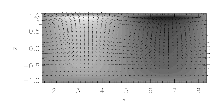
Figure 7: Field structure of the fastest growing mode for $B_{0}=2000$. Arrows: $b_{x,z}$, grey shading: value of $b_{y}$, dark – into, light – out of the plane.

5 Discussion and Conclusions

Clearly, any assignment of the results gained by help of a very simplified model to real neutron stars has to be done with great care. Even when accepting the plane layer as a reasonable approximation of the crust one has to concede that the very specific profile of $\@vec{B}_{0}$ assumed above may only exemplify the crustal field’s structure.

An acceptable approximation of the radial profile of a dipolar crustal field as given, e.g., in Page et al. (2000) will in general have to allow for non–zero values at the boundaries which cause a more complicated perfect conductor boundary condition. Moreover, the strong dependence of the conductive properties on the radial co–ordinate should anyway be taken into account.

Recently, Hollerbach & Rüdiger (2002) solved the non–linear Eq. (22) for the first time in a spherical shell geometry, again with the transport coefficients constant in space and time, and applying the vacuum and the perfect conductor boundary conditions at the surface and at the crust bottom, respectively. This is the best model for the non–linear magnetic field evolution in the crust of neutron stars available so far. They made different assumptions about the large–scale initial field (which corresponds in some sense to our background field) and report, as all the formerly mentioned authors too, about insurmountable numerical problems when the initial magnetization parameter, very roughly to be identified with $B_{0}$, exceeds $\approx 200$. Although their investigations can not reveal the existence and the character of the instability presented above (too short integration period in comparison with the growth time of the unstable modes for the maximum initial field considered), they found at least two features which support our results: For the largest feasible initial field their Legendre spectra are no longer convergent and indicate a local minimum at $l\approx 60$, a hint that small–scale field structures are fed in a non–cascade–like, possibly unstable way. Moreover, their findings confirm the importance of the background field’s profile curvature: For an initial (poloidal) field nearly linear in $r$ the excitation of small–scale structures and the acceleration of the decay were insignificant, in contrast to an initial (toroidal) field with a nearly quadratic $r$–profile.

To get an impression of possible consequences for the evolution of neutron stars we now simply assume, that the real $\@vec{B}$–profile is sufficiently “curved” (i.e., its second spatial derivative is big enough) and associate the parameter $B_{0}$ with a typical value of the field.

Assuming further electric conductivity and chemical composition to be constant, $\sigma_{0}=5\times 10^{26}$s^-1 and the relative atomic weight $A/Z=25$, respectively, we find the normalization field at a density $\rho=10^{14}$g cm^-3 to be $7\times 10^{10}$G (see, e.g., Page et al. 2000). That is, for typical (inner) crustal magnetic fields ranging from $7\times 10^{12}$G to $1.4\times 10^{14}$G we find a $B_{0}$ between $100$ and $2000$ and the e–folding time of the most rapidly growing unstable mode to be $0.0035$ and $0.0003$ times the ohmic decay time, respectively. Note, when comparing with the values of Fig. 5 that the dimensionless thickness 2 of the slab causes a factor 4 in the growth times. These values agree roughly with the ratios $\tau_{B}/\tau_{\text{ohm}}$ derived in Sect. 3 from observational data. An initial perturbation will quickly evolve to a level at which the linear analysis is no longer feasible, that is, at which it starts to drain a remarkable amount of energy out of the background field. Note, that the assumption about $B_{0}$ may well be in agreement with the surface field data given in Table 1.

We want to emphasize again that a sufficient curvature of the background field profile is a necessary condition for the occurrence of an unstable behavior. Therefore neither the derivation of the well–known helicoidal waves (whistlers) nor its modification presented in Vainshtein et al. (2000) could reveal it because a homogeneous background field was used there.

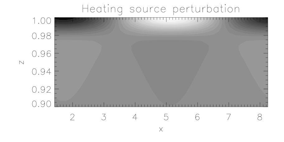
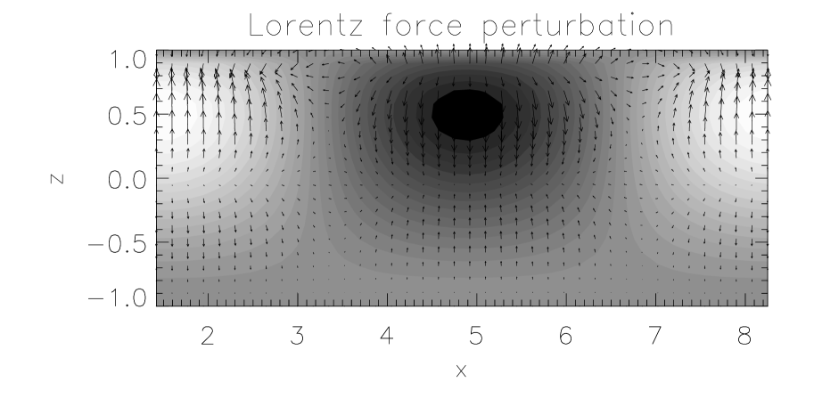
Figure 8: Heat source density perturbation $2\operatorname{curl}\@vec{B}_{0}\cdot\operatorname{curl}\@vec{b}$ (upper panel) and Lorentz force density perturbation $\operatorname{curl}\@vec{B}_{0}\times\@vec{b}+\operatorname{curl}\@vec{b}\times\@vec{B}_{0}$ (lower panel) of the fastest growing mode for $B_{0}=2000$ in arbitrary units. Upper panel: dark and light shading denotes cooling and heating by the perturbation, respectively; note the stretched $z$–scale. Lower panel: arrows denote $x$– and $z$–force components, grey shading the value of the $y$–component (dark – into, light – out of the plane).

With great reserve we may speculate about possible observational consequences. For SOINSs, the small–scale field modes initially generated or existing in the crust have already been decayed and the magnetic field is concentrated almost completely in the large–scale, say, dipolar mode. Simultaneously, in the process of cooling the coefficient $m_{e}^{*}c/e\tau_{e}$, i.e., the normalization field $B_{N}$, becomes smaller and smaller until the Hall–term in Eq. (22) dominates the linear ohmic term. Of course, as a counteracting tendency, the magnetic field decay will continue, increasingly modified by the Hall–cascade and the gradual onset of the Hall–instability. Therefore, we are confronted with a competition of one process increasing $B_{0}$ (via $\tau_{e}$) and another diminishing it (via the non–normalized magnetic field). The final decision whether $B_{0}$ indeed reaches values $O(1000)$ or even higher has to be left to non–linear coupled magneto–thermal calculations. Once the Hall–term dominates the instability may raise small–scale perturbations down to scale lengths $\gtrsim l_{\text{crit}}$ on expense of the dipolar mode, resulting in a spin–down behaviour of SOINSs as discussed in Sect. 3.

Another possible observational consequence follows from the dissipative effects of the rapidly excited small–scale field modes, that is, enhanced Joule heating. As can be seen in the upper panel of Fig. 8, the growing perturbations cause heat sources located close to the surface of the crust which, in turn, may produce a patchy neutron star surface. Note, that the plot shows only the part linear in $\@vec{b}$ of the heat source distribution, since the quadratic term $(\operatorname{curl}\@vec{b})^{2}$ has to be dropped in the linear analysis. These heat sources are concentrated in a very thin layer comprising only less than 5 % of the crustal thickness. Clearly, conclusions about the observability of that hot spots are impossible to be drawn from our simple model, since to infer the temperature distribution from the heat sources demands the knowledge of the absolute perturbation amplitudes. Anyway, we expect the neutron star’s surface to be warmer during the episode of the Hall–instability than standard cooling calculations predict.

Third, strong small–scale field components cause small–scale Lorentz forces. The lower panel of Fig. 8 shows that the maximum of the Lorentz force density perturbation is concentrated in deeper regions of the crust (at about 25 % of the thickness). From its pattern one may infer shear, both in $y$– and $z$– directions, to be the prevailing type of deformation. Thompson & Duncan (1995) discussed a scenario in which the helicoidal waves, being a consequence of the Hall–drift, ignite high energetic bursts by cracking the crust. From our results we can hope that the unstable modes of the Hall–instability act even more efficiently than the at best undamped, but never growing helicoidal waves can.

However, all the questions connected with the actual influences of the presented instability on spin–down, cooling and crust–cracking can be decided only by performing non–linear calculations in a realistic spherical–shell geometry taking into account a realistic density profile and chemical composition of the crust. On the other hand, the question at which field strength the action of the Hall–instability finally ceases, that is, the field decay is again overtaken by ohmic dissipation and, as a consequence, to which extent the distribution of observable pulsars in a $B$–$P$, better, in a $B$–$P$–$\tau_{\text{a}}$ diagram is possibly influenced, can again only be answered on the basis of realistic non–linear magneto–thermal simulations. Whether the scenario of an accelerated field decay is in agreement with the observed properties of the pulsar population can only be decided by help of a population synthesis as presented by Regimbau & de Freitas Pacheco (2001) applying a decay pattern with an initially slow decay followed by an episode of rapid decay and leading finally to a nearly constant field.