The Connection Between Spectral Evolution and GRB Lag

Abstract

The observed delay in the arrival times between high and low energy photons in gamma-ray bursts (GRBs) has been shown by Norris et al. to be correlated to the absolute luminosity of a GRB. Despite the apparent importance of this spectral lag, there has yet to be a full explanation of its origin. We put forth that the lag is directly due to the evolution of the GRB spectra. In particular, as the energy at which the GRB’s $\nu F_{\nu}$ spectra is a maximum ($E_{pk}$) decays through the four BATSE channels, the photon flux peak in each individual channel will inevitably be offset producing what we measure as lag. We test this hypothesis by measuring the rate of $E_{pk}$ decay ($\Phi_{o}$) for a sample of clean single peaked bursts with measured lag. We find a direct correlation between the decay timescale and the spectral lag, demonstrating the relationship between time delay of the low energy photons and the decay of $E_{pk}$. This implies that the luminosity of a GRB is directly related to the burst’s rate of spectral evolution, which we believe begins to reveal the underlying physics behind the lag-luminosity correlation. We discuss several possible mechanisms that could cause the observed evolution and its connection to the luminosity of the burst.

Introduction

Gamma-ray burst spectra have a well known property of evolving as the burst proceeds. This evolution is characterized by two distinct features: an overall softening of the GRB spectra with time and a delay in the arrival of low energy photons. Although GRBs show remarkable variety in most of their properties, such as duration and light curve structure, the evolution of the GRB spectra appears to be a universal trend that is observed in a large number of bursts.

Cheng et. al. (1995) first quantified the delay, or lag, of the low energy photons by using the cross-correlation technique to measure the difference in arrival times between high and low energy photon peaks. The authors used data collected by the BATSE instrument onboard the Compton Gamma-Ray Observatory, which for triggering purposes was typically subdivided into four broad energy channels from 25 keV to above 300 keV, each channel producing a different light curve for a particular GRB event. For example, the four energy dependant light curves for GRB 930612 are shown in Figure 1. When applied to timing analysis the cross-correlation function can be used to look for variable components between similar signals, which, for example, can yield correlation coefficients for the temporal offset between two photon light curves. Using this method Cheng et. al. found that almost all of the bursts they examined showed a delay in the 25-50 keV photon arrival times, which they attributed to scattering near the environment surrounding the GRB. Norris et. al. (2000) later used a similar approach of using a cross-correlation function (CCF) method to measure the lag between the BATSE channel 3 (100-300 keV) and channel 1 (25-50 keV) light curves for all GRBs with independently measured redshift. What they found was an anticorrelation between the delay in the low energy photon arrival times and the absolute luminosity of the GRB, yielding one of the first distance indicators that could be obtained from the gamma-ray data alone.

Figure 1: The light curve profile of GRB 930612 (BATSE trigger 2387) in four energy bands. There is a significant time delay of the soft energy photons.

They found that bursts with high luminosity exhibited little or no lag, whereas fainter bursts exhibited the largest time delay.

There have been ideas proposed to explain the lag-luminosity relationship based on viewing angles and kinematics (Solmonson 2001, Ioka 2000), but most of these do not try to address how the lag is produced but rather why the lag is connected to the peak luminosity. Thus the origin of GRB lag has largely been unexplained.

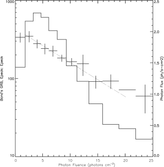
Figure 2: $E_{pk}$ vs. photon fluence for GRB 990712 (7648) plotted over the burst’s photon lightcurve. The decay constant is much more well defined for FRED bursts.

We put forth an explanation that was first proposed quantitatively by Brad Schaefer (in preparation astro-ph/0101462), namely that the observed spectral lag is directly related to the evolution of the GRB spectra to lower energies. Therefore, as the peak in the $\nu F_{\nu}$ spectra evolves through the various BATSE channels, the time to peak in the individual light curves will correlate to the hardness of $E_{pk}$. This softening of the GRB spectra has been known for some time (Golenetski et. al. 1983, Norris et. al. 1986) as a general hard to soft trend, but it was first quantified by Liang and Kargatis (1996) as an exponential decay of $E_{pk}$ as a function of photon fluence,

$$E_{pk}=E_{o}e^{-\Phi/\Phi_{o}}$$ (1)

where $E_{pk}$ is the max of the $\nu F_{\nu}$ spectra, and hence where most of the radiation energy is emitted, $\Phi(t)$ is the photon fluence integrated from the start of the burst, and $\Phi_{o}$ is the decay constant. In other words, the average energy of the arriving photons becomes softer as the burst progresses.

This simple interpretation of GRB lag predicts that the timescale of GRB spectral decay should correlate to the burst’s lag. There are several ways that this can be tested, but the most obvious would be to look for a correlation between the decay constant $\Phi_{o}$ of the $E_{pk}$ evolution and $\Delta t_{arrival}$ of the low and high energy photons. The decay constant represents the e-folding rate of the break energy and therefore can be used to parameterize the rate of evolution. It would be expected that the bursts that have the longest decays, and hence the smallest $\Phi_{o}$, would have the largest lag.

Figure 3: A 3 dimensional spectral plot of GRB 911016 (907) showing the hard to soft evolution of the peak energy. The solid line traces the decay of $E_{pk}$.

Data Analysis

In order to test the possible correlation between $E_{pk}$ decay rates and spectral lag we obtained the BATSE High Energy Resolution (HER) data for a sample of 19 GRBs. We then performed time-resolved spectral fits via $\chi^{2}$-minimization to the empirical Band model (Band et. al. 1993), allowing the high and low power law indices that characterize the Band spectral model to vary as free parameters. These 19 bursts were chosen because they are characterized by bright clean separable FRED (fast rise exponential decay) pulses which tend to give reliable $\Phi_{o}$ measurements. Bursts exhibiting multiple pulse structure on short timescales tend to have overlapping $E_{pk}$ decay periods, which complicates the measurement of the decay constant. For this reason, structured bursts were excluded from this analysis. An example of the time-resolved spectral fits that were performed is shown in Figure 2, where the log of $E_{pk}$ vs. photon fluence is plotted over the burst’s light curve which is shown in photons $cm^{-2}$ $s^{-1}$. The peak energy in 990712 can be seen to decay monotonically on the semi-log plot, and a linear fit to this trend directly yields $\Phi_{o}$.

The lag measurements where performed by using a simple cross-correlation (CCF) analysis between background subtracted BATSE low (25-50 keV) and high (100-300 keV) energy light curves, yielding the temporal offset of the two signals. The luminosities of these bursts were then calculated using the Norris et. al. lag-luminosity relation, which can be expressed as (Schaefer et. al. 2001):

$$L=2.51x10^{51}({\Delta t_{lag}/0.1})^{-1.14}$$ (2)

This relation gives the GRB peak luminosity as a function of intrinsic spectral lag at the source. Therefore, in order to obtain meaningful luminosities we need to correct the observed lag seen at the detector by a factor of $1+z$ for cosmological time dilation. Since we don’t have an a priori knowledge of the redshifts for our sample, we’ve employed an iteration routine that guesses an initial value for z and then converges upon the proper lag. This is done in the following manner: first an initial guess for $z$ is used to obtain $\Delta t^{\prime}=\Delta t_{obs}/(1+z)$, which in turn gives us an initial value for the luminosity. This is then used with the burst’s energy flux to obtain a value for the luminosity distance $D_{L}$ to the burst. This distance is then compared to the $D_{L}$ that can be calculated directly from $z$ assuming standard cosmological parameters ($H_{o}=65$ km s^-1, $\Omega=0.3$, $\Lambda=0.7$). The value for $z$ is then varied until the luminosity distances obtained from the two separate methods converge to within 1 part in 10³.

Figure 4: A plot of $\Phi_{o}$ vs. the GRB spectral lag for our entire sample. Note that the bursts with the fastest decay (lower $\Phi_{o}$) have the shortest lags.

It must be noted that of the seven bursts that Norris et. al. used to find Eq. 2, only one was a FRED event. This of course introduces an obvious caveat in our analysis, namely that we make the explicit assumption that the lag-luminosity relation holds for all bursts, including single peaked FREDs.

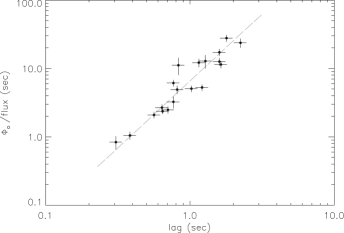
Figure 5: A plot of $\Phi_{o}/$flux vs. lag for 19 GRBs

Results

Figures 3 shows a 3 dimensional time resolved spectral plot for GRB 911016 (trigger 907), with time on the x-axis, BATSE LAD spectroscopic channel number on the y-axis and counts on the z-axis. Each slice in the yz-plane represents the GRB’s time resolved spectra, which in this case refers to a Band model fit to the BATSE high energy resolution data, whereas a cross section taken in the xz-plane reproduces the GRB light curve. In Figure 3, the evolution of the peak energy, which is represented by the solid line, can clearly be seen to begin at high energies and decay down to the BATSE detector threshold. The individual light curves that are used to measure the lag, typically those of channels 1 and 3, can be thought of as being cross sections along the xz-plane at the center of that channel’s energy range. For example, the channel 3 light curve, which corresponds to 100-300 keV, would be located in the middle of the y-axis. A cross section along the xz-plane taken at this point would give a light curve would be seen to peak very early in the burst. On the other hand, a slice taken at the 25-50 keV energy range which corresponds to the first few bins of the y-axis, would yield a light curve peak very late in the burst. We believe that this hard to soft evolution is the fundamental factor that contributes to the production of what we see as lag. If the decay in the above case was very short, then the time delay between the channel 3 and 1 light curves would be relatively small, but if the decay of $E_{pk}$ took several tens of seconds, then it’s expected that the low energy light curve would peak at a much later time. Note that it is not necessary for $E_{pk}$ to decay through all four channels, even if the peak energy were below 100 keV at the start of the burst, the peak in the channel 3 light curve would still occur very near the onset of the burst due to the geometry of the spectra.

Figure 4 shows a plot with the resulting $\Phi_{o}$ measurement vs. the spectral lag for our entire sample of bursts. A general trend can be seen that bursts with large $\Phi_{o}$ values result in longer lags, supporting the notion that longer $E_{pk}$ decay timescales lead to larger lags. A power law fit to the $\Phi_{o}$ vs. lag data reveals a nearly linear correlation of the two parameters with an index of 1.178 $\pm$ 0.058. In Figure 5, we’ve also plotted $\Phi_{o}$ normalized by the peak flux of the burst vs. lag, which has the units of seconds, thus giving a decay timescale in the detector frame. This seems to give a tighter correlation than simply $\Phi_{o}$ vs. lag, and a power law fit gives an index of 1.75. The motivations for this flux correction comes directly from the time derivative of the Liang-Kargatis relationship $dE_{pk}/dt=Flux/\Phi_{o}$.

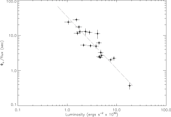
Figure 6: A plot of $\Phi_{o}/$ flux vs. Luminosity as found from the Norris et. al. lag-luminosity relation.

Because of the lag-luminosity relation, any correlation between $\Phi_{o}$ or $\Phi_{o}/$flux vs. lag inescapably leads to a discussion about a connection between spectral evolution and absolute luminosity. If the rate of spectral evolution is linearly correlated to lag, then it should be inversely correlated to the luminosity of the burst, assuming the validity of the lag-luminosity relation. To test this, we’ve calculated the luminosities, and hence the distances, for all 19 bursts in our sample using the method outlined in the previous section. The resulting luminosities have been plotted vs. $\Phi_{o}/$flux in Figure 6. Both the $\Phi_{o}$ and $\Phi_{o}/$flux relationships satisfy the expected anticorrelation, but the $\Phi_{o}/$flux vs. luminosity correlation provides a much tighter fit, ultimately yielding a higher statistical significance. These results directly imply that more luminous bursts tend to have faster rates of spectral evolution. It would also mean that a lower flux burst would have a wider pulse (larger lag) compared to a high flux burst with a similar rate of spectral decay. This leads to two noteworthy relationships, namely;

$$L=a_{0}\bigl{(}\frac{flux}{\Phi_{o}}\bigr{)}^{a_{1}}$$ (3)

which implies:

$$D_{L}=\bigl{[}\frac{a_{0}}{\Omega}\bigl{(}\frac{flux^{a_{1}-1}}{\Phi_{o}^{a_{1}}}\bigr{)}\bigr{]}^{-\frac{1}{2}}$$ (4)

where $\Omega$ is the beaming solid angle. A best fit to the $\Phi_{o}/$flux data gives an estimate of the $a_{0}$ coefficients to 9.8x10⁷² ergs cm^-2 $\pm$ 0.39 and a power law index of $a_{1}$ = 1.41 $\pm$ 0.06. Note that when $a_{1}$ = 1, we recover a simple relationship between the luminosity distance and the spectral decay constant:

$$D_{L}=(\frac{a_{0}}{\Omega\Phi_{o}})^{-\frac{1}{2}}$$ (5)

Where again, the beaming angle is left as an undetermined parameter, as a result, the data shown in Figures 6 and 7 are plotted per steradian. This leaves open the possibility that any perceived luminosity-$\Phi_{o}$ correlation may have been distorted by the lack of beaming angle information. The fact that we see any correlation however, and not simply a scatter plot, leads us to believe that the beaming angle distribution may actually be narrow for our sample, contributing to the overall spread in our results, but that it does not conceal the underlying correlations.

Discussion

The results shown in Figure 3 reveal that the spectral lag measured in GRB is directly connected to the hard to soft evolution of the burst spectra. This inescapably opens up a number of questions about the nature of the lag-luminosity correlation. If lag is directly proportional to the $E_{pk}$ decay constant $\Phi_{o}$, then the primary question is not why the GRB’s absolute luminosity is related to its lag, but rather why is it related to the burst’s rate of spectral evolution. We believe that this question is more fundamental, and ultimately needs to be addressed. To do so, we must first understand the mechanism that produces breaks in the GRB spectra and what causes its evolution. This, as it turns out, is a much harder question, because of the uncertainties involved with the microphysics of GRBs. The interpretation of $E_{pk}$ (and hence its evolution) depends on the radiation mechanism that is used to explain the GRB spectra. Here we attempt to review several mechanisms that could produce the GRB specra and discuss how the hard to soft evolution would be connected to the bursts luminosity for each model.

Liang and Kargatis originally proposed that the decay of $E_{pk}$ is governed by a confined plasma with a fixed number of particles $N$ cooling via $\gamma$-radiation. This type of exponential decay of the break energy with photon fluence that is seen in the Liang-Kargatis relation is expected if the average energy of the emitted photons is directly proportional to the average emitting particle energy such as in thermal bremsstrahlung or multiple Compton scattering. In this interpretation, the connection between luminosity and spectral evolution arises from simple energy conservation. If the energy budget of a GRB pulse is derived from a standard reservoir (Frail et. al. 2001), then more luminous bursts are radiating their energy away faster, resulting in a faster ”cooling” of their characteristic energy, hence a shorter lag. In this interpretation, the quantity $\Phi_{o}D_{L}^{2}$ would then represent the total number of radiating particles.

This cooling interpretation does not work as well when applied to the popular optically thin synchrotron model because the radiation cooling timescales alone are typically much too short. For example, if we interpret the average break energy of a GRB ($\sim E_{pk}$) as the characteristic energy of synchrotron self absorption, then the resulting magnetic field must be extremely high, about $\sim$ $1x10^{7}$ to $1x10^{8}$ Gauss. Separately, if we simply assume equipartition conditions then the magnetic field can be constrained as a function of lepton density, which, in most models, results in a field estimate of about $10^{5}$ to $10^{6}$ G. In either case, such high $B$ fields would create a synchrotron cooling timescale on the order of $10^{-5}$ seconds in the comoving frame (Wu and Fenimore 2000). This says that radiative cooling cannot be the sole process behind the production of the observed evolution.

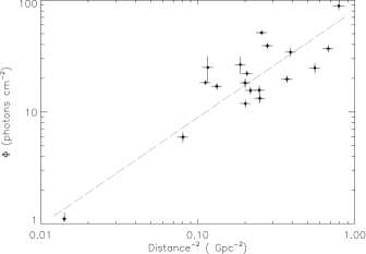
Figure 7: A plot of $\Phi_{o}$ vs. distance^-2

When considering the optically thin synchrotron model, the time variation of the burst’s internal parameters must be included namely the shell thickness $H$, $B$, the bulk Lorentz factor $\Gamma$, and the mean number of radiating particles $N$. It is not unlikely that these parameters will vary during the course of the burst. In the internal shock scenario faster moving shells in a relativistic outflow from the burst progenitor collide with slower moving shells and emit via optically thin synchrotron radiation. This tells us two things, that the peak emission can be expressed as $E_{pk}\propto\gamma^{2}B$ and that $d\Gamma/dr<0$. Therefore, as the shells expand outward, the bulk Lorentz factor $\Gamma$ will decrease resulting in a lower observed frequency of peak emission. This effect becomes important when considering successive episodes of emission within the same bursts, but the variation of $\Gamma$ is likely to be small on the timescale of an individual pulse and hence can be considered a constant during single periods of emission.

This leaves the size of the emitting region and the magnetic field. It is expected that the size of the emitting plasma will expand in thickness once the forward and reverse shocks propagate through the plasma. If an initial magnetic flux is frozen into the plasma, either from the progenitor or after turbulent field growth at the shock front, then the field strength should be inversely proportional to the shell thickness, ($B\propto H^{-1}$), assuming that the shells are thin. Therefore an increase in the size of the radiating plasma will lower the magnetic field and hence shift the synchrotron spectra to lower energies (e.g., Tavani 1996). Since both the forward and reverse shocks travel close to the speed of light (i.e. $B\propto 1/ct$), this mechanism can easily alter the spectra on the observed timescale. Furthermore, since $E_{pk}\propto\gamma^{2}B$ and $F_{E}\propto\gamma^{2}B^{2}$, we can recover the Liang-Kargatis relationship (Eq. 1) in a self consistent manner, as long as the shells can be considered thin compared to their overall size. In this interpretation the connection between luminosity and spectral evolution comes directly from initial magnetic field strength and its decay with time. Bursts that are intrinsically more luminous start with large magnetic fields, causing their decay timescales to be short. This is not unlike the previous interpretation given for the inverse Compton case, except that now the initial variations in the magnetic field strength give rise to the distribution in burst luminosity.

This interpretation again relies on the cooling of the radiating leptons as a critical timescale, which is problematic since if the magnetic field is indeed as large as that estimated earlier, then the radiating particles would have lost all of their energy well before the expansion of the shell takes place. This is representative of a larger problem with the high $B$ field synchrotron model, namely that the cooling timescale is much shorter then the observed variations (i.e. spikes) of emission in GRB pulses. Synchrotron self Compton and Synchrotron self absorption are two models that could produce the GRB spectra with much smaller magnetic fields and hence avoid this cooling problem while producing evolution on the observed timescale. Furthermore, curvature effects of a relativistically expanding shell can also produce spectral break evolution without having to be constrained by the burst’s cooling timescale, allowing for high magnetic fields. A more detailed analysis of the causes behind spectral evolution for a wider range of emission models, including the contribution of curvature effects, will be reserved for a future paper.

Finally, we’d like to return to the idea of a standard energy reseviour in GRBs reported by Frail et. al 2000. It can be shown (Kocevski $\&$ Liang 2002) that if the energy release rate is a constant during the prompt emission, then by means of the energy conservation we know that if the burst is losing energy via radiation then:

$$\frac{-dE(t)}{dt}\propto L$$ (6)

and if we apply the empirical Liang-Kargatis relation, then

$$\frac{-dE_{pk}}{dt}=\frac{F_{E}}{\Phi_{o}}=\frac{L}{\Omega\Phi_{o}d^{2}}$$ (7)

If the total energy release is constant for GRB events, then this would imply that the quantity $\Phi_{o}$d² would be a constant for different bursts. Kocevski $\&$ Liang (2002) have recently reported evidence that supports this for a sample of FRED bursts. The constancy of $\Phi_{o}$d² can be also expressed as:

$$L\propto\frac{1}{\Omega}\frac{Flux}{\Phi_{o}}$$ (8)

Which is simply the $\Phi_{o}$-luminosity anticorrelation obtained empirically in equation 3 with $a_{1}$=1. To test the relationship given in Equation 6, we’ve plotted $\Phi_{o}$ vs. $D_{L}^{-2}$ for our current sample of bursts in Figure 7. From this we can see that the data is consistent with a linear correlation, with a best fit giving a power law index of 0.884. Therefore, having the energy release per steradian in a GRB come from a standard energy budget that is common among GRB events is consistent with our results.

REFERENCES

Band, D., et al. 1993. ApJ, 428, 21
Cheng, L. X., et. al., 1995, A$\&$A, 300, 746
Crider et. al. 1997, ApJ, 479, L39
Golensetski, S. V. et al. 1983, Nature, 306, 451
Frail, D. A., et. al. 2001, ApJ, 562, L55
Ioka et. al. 2001 ApJ 554L, 163I
Liang, E., $\&$ Kargatis, V. 1996. Nature, 381, 49
Kocevski, D., $\&$ Liang, E., 2002, submitted, AIP Conf. Proc, Woods Hole GRB conference
Norris, J. P., et. al. 1986, Apj, 301, 213
Norris, J. P., et al. 2000, ApJ, 534, 248
Salmonson, J. 2000. ApJ, 544L, 115S
Schaefer, B. et. al. in preparation astro-ph/0101462
Tavani, M., 1996, ApJ, 466, 768
Wu $\&$ Fenimore, 2000, Apj, 535, 29