Separating the Early Universe from the Late Universe:
cosmological parameter estimation beyond the black box

Abstract

We present a method for measuring the cosmic matter budget without assumptions about speculative Early Universe physics, and for measuring the primordial power spectrum $P_{*}(k)$ non-parametrically, either by combining CMB and LSS information or by using CMB polarization. Our method complements currently fashionable “black box” cosmological parameter analysis, constraining cosmological models in a more physically intuitive fashion by mapping measurements of CMB, weak lensing and cluster abundance into $k$-space, where they can be directly compared with each other and with galaxy and Ly$\alpha$ forest clustering. Including the new CBI results, we find that CMB measurements of $P(k)$ overlap with those from 2dF galaxy clustering by over an order of magnitude in scale, and even overlap with weak lensing measurements. We describe how our approach can be used to raise the ambition level beyond cosmological parameter fitting as data improves, testing rather than assuming the underlying physics.

]

I Introduction

What next? An avalanche of measurements have now lent support to a cosmological “concordance model” whose free parameters have been approximately measured, tentatively answering many of the key questions posed in past papers. Yet the data avalanche is showing no sign of abating, with spectacular new measurements of the cosmic microwave background (CMB), galaxy clustering, Lyman $\alpha$ forest (Ly$\alpha$F) clustering and weak lensing expected in coming years. It is evident that many scientists, despite putting on a brave face, wonder why they should care about all this new data if they already know the basic answer. The awesome statistical power of this new data can be used in two ways:

1. To measure the cosmological parameters of the concordance model (or a replacement model if it fails) to additional decimal places

2. To test rather than assume the underlying physics

This paper is focused on the second approach, which has received less attention than the first in recent years. As we all know, cosmology is littered with “precision” measurements that came and went. David Schramm used to hail Bishop Ussher’s calculation that the Universe was created 4003 b.c.e. as a fine example — small statistical errors but potentially large systematic errors. A striking conclusion from comparing recent parameter estimation papers (say [1, 2, 3, 4] by the authors for methodologically uniform sample) is that the quoted error bars have not really become smaller, merely more believable. For instance, a confidence interval for the dark energy density that would be quoted three years ago by assuming that four disparate data sets were all correct [1] can now be derived from CMB + LSS power spectra alone [4, 5, 6, 7] and independently from CMB + SN 1a as a cross-check.

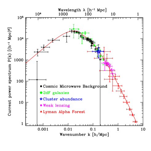
FIG. 1.: Measurements of the linear matter power spectrum $P(k)$ computed as described in the text, using the concordance model of [5] (solid curve) to compute window functions. The locations of the CMB points depend on the matter budget and scales with the reionization optical depth as $e^{2\tau}$ for $k\mathrel{\hbox to0.0pt{\lower 3.0pt\hbox{$\mathchar 536\relax$}\hss}\raise 2.0pt\hbox{$\mathchar 318\relax$}}0.002$. Correcting for bias shifts the 2dF galaxy points [8] vertically ($b=1.3$ assumed here) and should perhaps blue-tilt them slightly. The cluster point scales vertically as $(\Omega_{m}/0.3)^{-1.2}$, and its error bars reflects the spread in the literature. The lensing points are based on [9]. The Ly$\alpha$F points are from a reanalysis [10] of [11] and have an overall calibration uncertainty around 17%.

This paper aims to extend this trend, showing how measurements can be combined to raise the ambition level beyond simple parameter fitting, testing rather than assuming the underlying physics. Many of the dozen or so currently fashionable cosmological parameters merely parametrize two cosmological functions [12, 13]: the cosmic expansion history $a(t)$ and the cosmic clustering history $P(k,z)$, the observables corresponding to 0th and 1st order cosmic perturbation theory, respectively. This means that non-parametric measurements of these cosmological functions allows testing whether the assumptions associated with the cosmological parameters are in fact valid. Moreover, if there are discrepancies, comparing measurements of these functions from different data sets reveals whether the blame lies with theory, data or both.

We will limit our treatment to the 1st order function, $P(k,z)$, since the 0th order function has been extensively discussed previously [12, 13, 14]. One of the key ideas of this paper is summarized in Figure 1, showing how CMB, LSS, clusters, weak lensing and Ly$\alpha$F all constrain $P(k,z)$ at $z=0$. The first plots that we are aware of showing CMB in k-space go back a decade [15], when CMB merely probed scales much larger than accessible to large-scale structure measurements. Since then, CMB has gradually pushed to smaller scales with improved angular resolution while LSS has pushed to larger scales with deeper galaxy surveys. What is particularly exciting now, and makes this paper timely, is that the two have met and overlapped, especially with the CBI experiment [16] and the 2dF [17] and SDSS [18] redshift surveys. Figure 1 shows that CMB now overlaps also with the scales probed by cluster abundance and even, partly, with weak lensing.

$P(k,z)$ can be factored as the product of a primordial power spectrum $P_{*}(k)$ and a transfer function, corresponding to the physics of the Early Universe and the Late Universe, respectively. The two involve completely separate physical processes and assumptions that need to be tested, and the purpose of our method is to measure these two factors separately using observational data. Given a handful of cosmological parameters specifying the cosmic matter budget and the reionization epoch, the transfer function can be computed from first principles using well-tested physics (linearized gravity and plasma physics at temperatures similar to those at the solar surface). The primordial power spectrum is on shakier ground, generally believed to have been created in the Early Universe at an energy scale never observed and involving speculative new physical entities. Most work has parametrized this function as a power law $P_{*}(k)\propto k^{n}$ or a logarithmic parabola $P_{*}(k)\propto k^{n+\alpha\ln k}$, inspired by the slow-roll approximation in inflationary models [19], usually with $\alpha=0$. More general parametrizations have included broken power laws [20, 21, 22, 23] a piecewise constant function [24] and other forms [25, 26]. It has also been shown [24] that the MAP CMB data [27] in combination with SDSS power spectrum measurements should be able to constrain the shape of $P_{*}(k)$ in considerable detail. The key challenge is breaking the degeneracy between the two factors, $P_{*}(k)$ and the transfer function. Although a future brute-force likelihood analysis parametrizing $P_{*}(k)$ with, say, 20 parameters would be interesting and perfectly valid, it would obscure the simplicity of the underlying physics. Such a “black box” approach would entail computing many different curves for each point in parameter space (such as $C_{\l}$ for CMB, $P(k)$ for galaxies, the aperture mass function $M_{\rm app}(\theta)$ for lensing and the cluster mass function), and mapping out the 20-dimensional likelihood function numerically by marginalizing over other cosmological parameters like those of the matter budget. This would be overkill, since (modulo nonlinearity complications treated below) all measurements shown in Figure 1 can be recast directly as weighted averages of $P_{*}(k)$.

The rest of this paper is organized as follows. In Section II, we describe the construction of Figure 1, explaining how CMB, weak lensing and cluster abundance measurements can be mapped into (linear) $k$-space. In Section III, we turn to the degeneracy between $P_{*}(k)$ and cosmological parameters such as the various matter densities, and present our method for breaking it. We show how this allows measuring the cosmic matter budget without assuming anything about $P_{*}(k)$ and obtaining a non-parametric measurement of $P_{*}(k)$.

II Measuring $P(k)$ when the transfer functions are known

In this section, we discuss how measurements of CMB, weak lensing, cluster abundance, Ly$\alpha$F and galaxy clustering probe $P(k)$ and $P_{*}(k)$ when the relevant transfer functions are known. We will see that in all five cases, each measured data point $d_{i}$ (a CMB band power $\delta T_{\l}^{2}$, a lensing aperture mass variance $\langle M_{\rm app}(\theta)^{2}\rangle$, etc.) can be written as an integral

$$d_{i}=\int_{-\infty}^{\infty}{\cal P}_{i}(k)d\ln k$$ (1)

over (linear) wavenumber $k$ for some non-negative integrand ${\cal P}_{i}(k)$. Renormalizing ${\cal P}_{i}(k)$ to be a probability distribution, our convention $(\star)$ in Figure 1 is the following:

• Plot the data point at the $k$-value corresponding to the median of this distribution with a horizontal bar ranging from the 20th to the 80th percentile.

These percentiles correspond to the full-width-half-maximum for the special case of a Gaussian distribution. In other words, the horizontal bars indicate the range of scales $k$ contributing to the data point. All transfer functions in this section are computed assuming the flat $\Lambda$CDM concordance model of [5] — we return the more general case in the next section. This is a flat, scalar, scale-invariant model with cold dark matter density $h^{2}\Omega_{m}=0.12$, baryon density $h^{2}\Omega_{b}=0.021$ and cosmological constant $\Omega_{\Lambda}=0.71$. This corresponds to a Hubble parameter $h=0.70$. We chose a reionization optical depth $\tau=0.05$, which corresponds to reionization at redshift $z=8$ with these parameters. We normalize the model to have $\sigma_{8}=0.815$, which provides a good fit to the CMB data.

A CMB data

Figure 2 shows all 119 CMB detections currently available, extending the compilation in [4] by adding the new measurements from the Very Small Array (VSA) [28] and the Cosmic Background Imager (CBI) mosaic [16]. Recent data reviews include [29, 30].

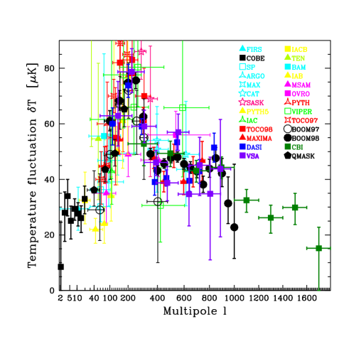
FIG. 2.: CMB data used in our analysis. Error bars in the plot do not include calibration or beam errors which allow substantial vertical shifting and tilting for some experiments (these effects were included in our analysis).

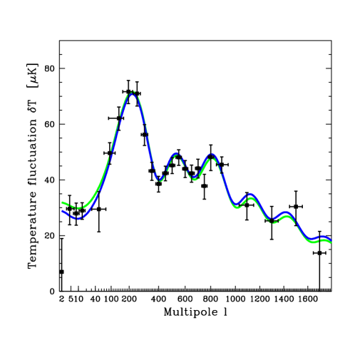
FIG. 3.: Combination of data from Figure 2. These error bars include the effects of beam and calibration uncertainties, which cause long-range correlations of order 5%-10% over the peaks. In addition, points tend to be anti-correlated with their nearest neighbors, typically at the level of a few percent. The horizontal bars give the characteristic widths of the window functions (see text). The curves show the flat $\Lambda$CDM concordance models from [4] (green/light gray) and [5] (blue/dark gray).

We combine these measurements into a single set of 25 band powers shown in Figure 3 and Table 1 using the method of [4], including calibration and beam uncertainties, which effectively calibrates the experiments against each other. The coefficients $y_{i}$ in equations (A2), (A4) and (A5) of [4] should strictly speaking be the window-convolved true power spectrum, so rather than approximating them by the observed data points as in [4], we approximate them by the the smooth fit to the data given by the green/light gray curve in Figure 3 convolved with the experimental window functions. We have excluded the PythV data since it disagrees with numerous other experiments on large angular scales and the non-release of the underlying map precludes clarifying this situation. Since our compressed band powers $d_{\l}$ are simply linear combinations of the original measurements, they can be analyzed ignoring the details of how they were constructed, being completely characterized by a window matrix ${\bf W}$:

$$\langle d_{i}\rangle=\sum_{\l}{\bf W}_{i\l}{\cal C}_{\l},$$ (2)

where ${\cal C}_{\l}\equiv\delta T_{\l}^{2}\equiv\l(\l+1)C_{\l}/2\pi$ and $C_{\l}$ is the angular power spectrum. This matrix is available at $www.hep.upenn.edu/{\sim}max/cmb/experiments.html$ together with the 25 band powers $d_{\l}$ and their $25\times 25$ covariance matrix. Following the convention used in Figure 1, the data $\l$-values and effective $\l$-ranges in Figure 3 and Table 1 correspond to the median, 20th and 80th percentile of the window functions ${\bf W}$. (We use absolute values of the window function to be pedantic, since some windows go slightly negative in places as a result of the inversion, although this makes a negligible difference for the plot.) Comparing Table 1 with the older results from [4], we find that the degree-scale normalization is marginally higher. In bin 8, for instance, corresponding to the 1st peak, the normalization has risen by 3% due to the inclusion of the VSA and CBI results and a further 6% due to the above-mentioned improved modeling of calibration and beam errors. With the old modeling, a measurement scattering low by chance would be assigned a smaller error and therefore get more statistical weight, pulling the overall calibration down somewhat. A detailed discussion of calibration issues can be found in [31].

Table 1 – Band powers combining the information from CMB data from Figure 2. The 1st column gives the $\l$-bins used when combining the data, and can be ignored when interpreting the results. The 2nd column gives the medians and characteristic widths of the window functions as detailed in the text. The error bars in the 3rd column include the effects of calibration and beam uncertainty. The full $25\times 25$ correlation matrix and $25\times 2000$ window matrix are available at $www.hep.upenn.edu/\sim max/cmb/experiments.html$.

$\l$-Band	$\l$-window	$\delta T^{2}\>[\mu$K${}^{2}]$
$2-2$	$2_{-0}^{+0}$	$49\pm 310$
$3-5$	$4_{-1}^{+2}$	$878\pm 308$
$6-10$	$8_{-2}^{+3}$	$782\pm 219$
$11-30$	$14_{-3}^{+4}$	$840\pm 171$
$31-75$	$51_{-20}^{+26}$	$869\pm 412$
$76-125$	$93_{-24}^{+26}$	$2457\pm 383$
$126-175$	$140_{-52}^{+26}$	$3854\pm 520$
$176-225$	$195_{-34}^{+26}$	$5130\pm 595$
$226-275$	$250_{-24}^{+23}$	$5036\pm 613$
$276-325$	$300_{-22}^{+23}$	$3163\pm 423$
$326-375$	$352_{-20}^{+21}$	$1869\pm 278$
$376-425$	$399_{-20}^{+20}$	$1486\pm 216$
$426-475$	$451_{-20}^{+21}$	$1795\pm 221$
$476-525$	$500_{-20}^{+21}$	$2043\pm 260$
$526-575$	$550_{-21}^{+21}$	$2312\pm 271$
$576-625$	$601_{-20}^{+21}$	$1936\pm 269$
$626-675$	$650_{-21}^{+21}$	$1792\pm 261$
$676-725$	$700_{-20}^{+20}$	$1950\pm 295$
$726-775$	$750_{-21}^{+22}$	$1429\pm 336$
$776-825$	$802_{-21}^{+23}$	$2322\pm 440$
$826-1000$	$890_{-44}^{+51}$	$2065\pm 261$
$1001-1200$	$1094_{-63}^{+56}$	$955\pm 300$
$1201-1400$	$1299_{-54}^{+54}$	$639\pm 291$
$1401-1600$	$1501_{-54}^{+53}$	$925\pm 368$
$1601-\infty$	$1700_{-53}^{+51}$	$190\pm 273$

The angular power spectrum of the CMB is determined by the primordial power spectrum $P_{*}(k)$ through a linear relation

$${\cal C}_{\l}=\int_{-\infty}^{\infty}W_{\l}(k)P_{*}(k)d\ln k,$$ (3)

where the transfer functions $W_{\l}(k)$ depend on the cosmic matter budget and the reionization optical depth. Since

$$P(k)=T(k)^{2}P_{*}(k)$$ (4)

where $T(k)$ is the matter transfer function, equation (3) can be reexpressed directly in terms of the current power spectrum:

$${\cal C}_{\l}=\int_{-\infty}^{\infty}{W_{\l}(k)\over T(k)^{2}}P(k)d\ln k.$$ (5)

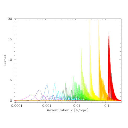
FIG. 4.: The curves $kW_{\l}(k)$ whose integral give ${\cal C}_{\l}$ for a scale-invariant spectrum, all rescaled to have unit area. From left to right, the curves are for multipoles $\l=2$, 4, 8, 16, 32, 64, 128, 256, 512, 1024.

Equation (3) implies that for the CMB with data points $d_{\l}\equiv{\cal C}_{\l}$, the integrand of equation (1) is simply ${\cal P}_{\l}(k)=W_{\l}(k)P_{*}(k)$. We compute the integral kernels $W_{\l}(k)$ with CMBfast [32]. Figure 4 shows ${\cal P}_{\l}(k)$ for a sample of $\l$-values, normalized to integrate to unity, for a scale-invariant primordial power spectrum $P_{*}(k)\propto k$. In other words, the figure simply shows $kW_{\l}(k)$ rescaled, the integral of which gives ${\cal C}_{\l}$. For each such curve, we compute the 20th, 50th and 80th percentile as per the above-mentioned convention $(\star)$ and plot the results in Figure 5 as an indication of what $k$-range is probed by each multipole $\l$. The situation is completely analogous for the polarization case. The relations between $\l$ and $k$ are seen to be roughly linear as expected, and to tighten with increasing $\l$.

The slight wiggles roughly line up with the derivatives of the three CMB power spectra. This is because when the power spectrum is steeply rising, the contribution will be larger from the peak on the right than from the trough on the left, pushing the median up towards higher $k$, and vice versa. These wiggles are seen to be more pronounced for E-polarization than for the unpolarized case. This is because the wiggles are sharper and have greater relative amplitude for the polarized case, increasing the magnitude of the derivative. The T-spectrum has milder wiggles since the peculiar velocity contribution fills in the troughs between the peaks from the dominant density/gravitational contribution — the E-power spectrum has only a velocity contribution and thus drops near zero between peaks, staying positive only because of geometric projection effects in the mapping from $k$-space to $\l$-space.

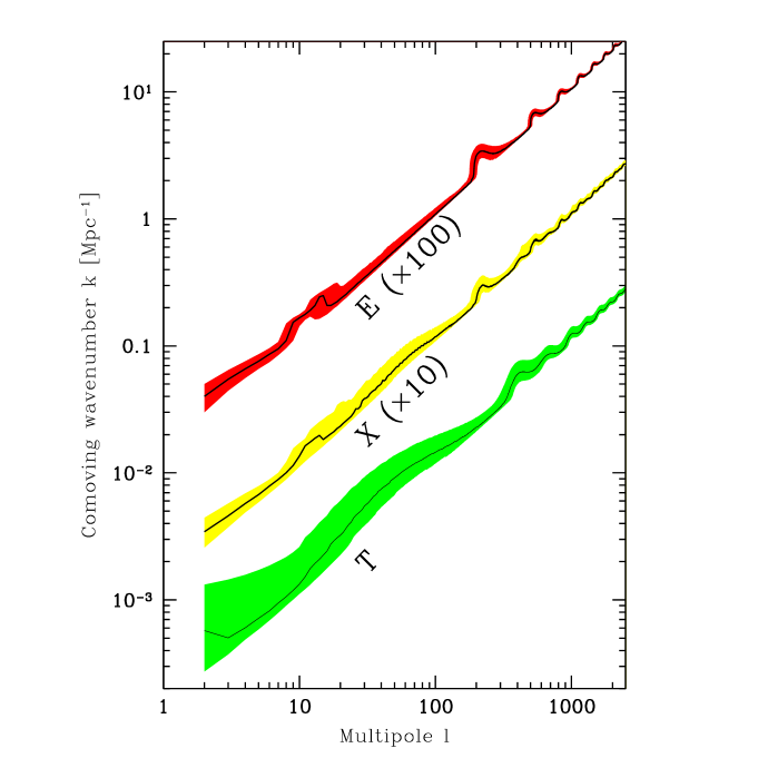
FIG. 5.: The correspondence between $\l$-space and $k$-space for CMB. For each $\l$, the shaded bands indicates the $k$-range from the 20th to 80th percentile of the distribution $kW_{\l}(k)$ (Figure 4), and the black curve shows the median. From top to bottom, the three bands are for the E-polarization, cross-polarization (X) and unpolarized (T) cases, respectively. To avoid clutter, the E and X bands have been multiplied by 10 and 100, respectively.

Because of incomplete sky coverage, real-world CMB measurement can never measure individual multipoles $\l$, merely weighted averages of many. Substituting equation (3) into equation (2) gives

$$\langle d_{i}\rangle=\int_{-\infty}^{\infty}W_{i}(k)P_{*}(k)d\ln k,$$ (6)

where

$$W_{i}(k)\equiv\sum_{\l}{\bf W}_{i\l}W_{\l}(k).$$ (7)

In other words, each of our 25 binned CMB measurements probes a known linear combination of the primordial power spectrum. A sample of these new window functions are plotted in Figure 6, and are again seen to be quite narrow for large $\l$. Indeed, although the $\l$-smearing makes these windows slightly broader than those in Figure 4, it is also seen to make them more well-behaved, eliminating the high-frequency oscillations at large $\l$.

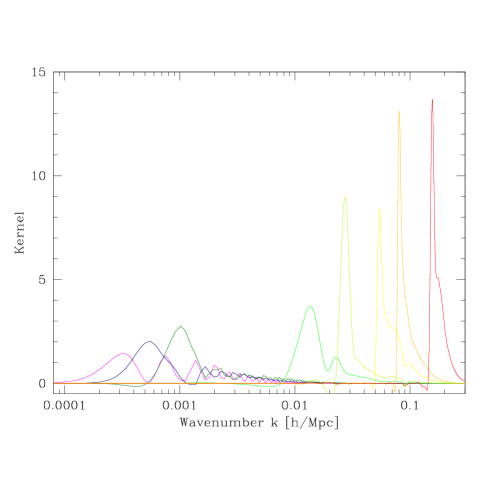
FIG. 6.: Sample curves $kW_{i}(k)$ whose integral give our binned CMB band powers from Figure 3 for a scale-invariant spectrum, all rescaled to have unit area. From left to right, the curves correspond to band powers $i=1$, 2, 3, 6, 9, 14, 19, 24.

We are now ready to map our CMB measurements from Figure 3 into $k$-space. We need a prescription for where to position the points both horizontally and vertically. Horizontally, we simply follow the above-mentioned convention $(\star)$ and plot it at the median of the distribution ${\cal P}_{i}(k)=kW_{i}(k)$ from Figure 6, with horizontal bars extending from the 20th to the 80 percentile. Vertically, we plot it at the value $\widehat{P_{*}}_{i}$ defined by

$$k^{-1}\widehat{P_{*}}_{i}\equiv{d_{i}\over\int_{-\infty}^{\infty}kW_{i}(k)d\ln k}.$$ (8)

Taking the expectation value of this and using equation (6) tells us that we can interpret $\widehat{P_{*}}_{i}$ as measuring simply a weighted average of $k^{-1}P_{*}(k)$ (which we expect to be a nearly constant function), with the window function $kW_{i}(k)$ giving the weights. The resulting 25 measurements of $P_{*}(k)$ are shown in Figure 7, and Figure 8 shows a simulation for measurements by the MAP satellite[27]. To plot these points as measurements of $P(k)$, we proceed analogously. We use exactly the same convention ($\star$) for the horizontal placement of the points, and given equation (4) plot them at a vertical position given by

$$\widehat{P}\equiv T(k_{\rm eff})^{2}\widehat{P_{*}},$$ (9)

where $k_{\rm eff}$ is the horizontal location of the point (the median of the window function). This allows us to interpret $\widehat{P}_{i}/P_{\rm fid}$ as measuring simply a weighted average of the relative power $P(k)/P_{\rm fid}(k)$, where $P_{\rm fid}(k)\equiv kT(k)^{2}$ is our fiducial power spectrum. This procedure produces the CMB points plotted in Figure 1 and Figure 9.

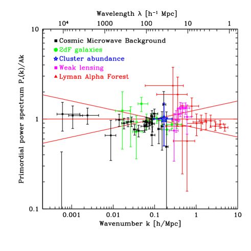
FIG. 7.: Measurements of the primordial power spectrum $P_{*}(k)$ computed as described in the text, divided by our fiducial primordial power spectrum $Ak$ with $A\approx(43.2{\rm Mpc}/h)^{4}$. This normalization corresponds to an rms fluctuation in the gravitational potential $\psi$ given by $[k^{3}P_{\psi}(k)/2\pi^{2}]^{1/2}=2.9\times 10^{-5}$. The data are the same as in Figure 1, divided by $AkT(k)^{2}$.

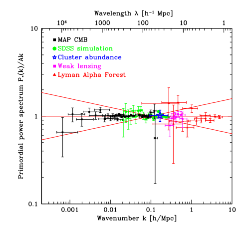
FIG. 8.: Same as Figure 7, but for simulated future data. CMB and galaxy points assume the advertized specifications for the complete MAP and SDSS datasets, respectively. The CMB simulation assumes the MID foreground model of [33]. Still better galaxy measurements are likely to result adding the SDSS luminous red galaxy survey [34] and photometric redshift information. The cluster point assumes a relative error of 7.5% on $\sigma(R)$, i.e., that systematic uncertainties can be reduced to the level of current statistical errors. The lensing and Ly$\alpha$F points assume that the current errors have been cut in half.

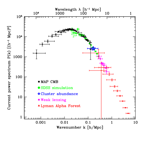
FIG. 9.: Same as Figure 8, but for the current linear power spectrum $P(k)$. In other words, this is Figure 1 for simulated future data.

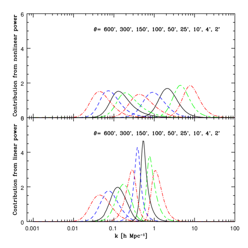
FIG. 10.: Curves show ${\cal P}^{\rm nl}(k)$ (top) and ${\cal P}^{\rm l}$ (bottom), normalized to have unit area. These curves show how much different nonlinear (top) and linear (bottom) scales contribute to the observed weak lensing aperture mass variance $\langle M_{\rm app}(\theta)^{2}\rangle$ for the source redshift distribution of [9] .

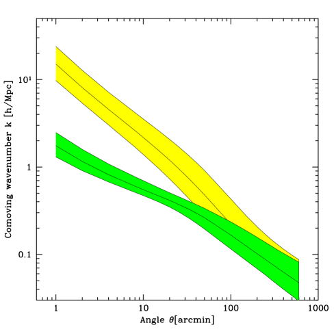
FIG. 11.: Ranges of $k$ that contribute to $M_{app}(\theta)^{2}$ as a function of $\theta$. The line indicates the median $k$ and the boundaries correspond to the 20th and 80th percentile. The upper (lower) band shows the range for nonlinear (linear) scales.

B Weak lensing data

Weak gravitational lensing uses photons from distant galaxies as test particles to measure the metric fluctuations caused by intervening matter, as manifested by distorted images. The first detections of this cosmic shear signal [35, 36] were reported in 2000 [37, 38, 39, 40, 41, 42], and dramatic improvements are likely to lie ahead just as for CMB observations. For this paper, we will use the results from the Red-Sequence Cluster Survey (RSCS) reported in [9], which includes data from a record-breaking 53 square degree sky area. We use the seven data points employed for the cosmological analysis in [9], i.e.,

$$d_{i}\equiv\langle M_{\rm app}(\theta_{i})^{2}\rangle$$ (10)

where $\theta=$10’, 15’, 20’, 25’, 35, 33, 42’, 50’. This measured quantity, denoted the aperture mass variance, is on average given by

$$\langle d_{i}\rangle=2\pi\int_{0}^{\infty}\left[{12J_{4}(\l\theta_{i})\over\pi(\l\theta_{i})^{2}}\right]^{2}\l P_{\kappa}(\l)d\l,$$ (11)

where $J_{4}$ is a Bessel function and $P_{\kappa}(\l)$ is the cosmic shear power spectrum. The shear power spectrum in turn is given by a linear combination of the nonlinear matter power spectrum $P_{\rm nl}(k_{\rm nl})$ over a range of wavenumbers $k_{\rm nl}$ and redshifts [35, 36],

$$P_{\kappa}(\l)={9\Omega_{m}^{2}H_{0}^{4}\over 4c^{4}}\int_{0}^{\omega_{H}}\left({\bar{W}(\omega)\over a(\omega)}\right)^{2}P_{\rm nl}\left({l\over f_{K}(\omega)};\omega\right)d\omega.$$ (12)

where we have introduced the comoving radial coordinate $\omega$ and $\omega_{H}$ corresponds to the horizon. Here $f_{K}(\omega)$ is the angular diameter distance and $\bar{W}(\omega)$ is a source-averaged ratio of angular diameter distances. For a given redshift distribution of the sources $p_{b}(\omega)$,

$$\bar{W}(\omega)=\int_{\omega}^{\omega_{H}}p_{b}(\omega^{\prime}){f_{K}(\omega^{\prime}-\omega)\over f_{K}(\omega^{\prime})}d\omega^{\prime}.$$ (13)

We use the best fit redshift distribution for the RSCS sample from [9],

$$p_{b}(z)={\beta(z/z_{s})^{\alpha}\over z_{s}\Gamma[(1+\alpha)/\beta}e^{-(z/z_{s})^{\beta}}$$ (14)

with $(\alpha,\beta,z_{s})=(4.7,1.7,0.302)$. With a change of variables to $k_{\rm nl}=\l/f_{K}(\omega)$ we can rewrite equation (11) in the form of

$$d_{i} = \int_{-\infty}^{\infty}{\cal P}^{\rm nl}_{i}(k_{\rm nl})d\ln k_{\rm nl}$$ (15)

$${\cal P}^{\rm nl}_{i}(k_{\rm nl}) = {9\Omega_{m}^{2}H_{0}^{4}\over 2\pi c^{4}}\int_{0}^{\omega_{H}}\left({\bar{W}(\omega)f_{K}(\omega)\over a(\omega)}\right)^{2}k_{\rm nl}^{2}P_{\rm nl}\left(k_{\rm nl};\omega\right)$$ (17)

$$\times\left[{12J_{4}(k_{\rm nl}f_{K}(\omega)\theta_{i})\over(k_{\rm nl}f_{K}(\omega)\theta_{i})^{2}}\right]^{2}d\omega.$$

The integrand ${\cal P}^{\rm nl}_{i}(k_{\rm nl})$ is an integral over cosmic time that depends linearly on the nonlinear matter power spectrum $P_{\rm nl}(k_{\rm nl})$ at various redshifts. The upper panel in Figure 10 shows this integrand for a sample of angular scales $\theta$. Just as for the CMB, we follow our convention $(\star)$ and compute the 20th, 50th and 80th percentiles of these distributions. The results, plotted in Figure 11, show that we approximately have $k\propto 1/\theta$ as expected but that the relation is not particularly tight, with a given $\theta$ probing a broad range of $k$-values.

To use this relation between $k$ and $\theta$ to map the lensing data into (linear) $k$-space would be quite misleading, since the nonlinear power $P_{\rm nl}(k_{\rm nl})$ is the result of gravitational collapse and therefore carries information about the linear power on larger spatial scales [43, 44, 45]. We will use the Ansatz of Peacock & Dodds [45] to quantify this effect. Defining

$$\Delta(k)={4\pi k^{3}\over(2\pi)^{3}}P(k),\quad\Delta_{\rm nl}(k_{\rm nl})={4\pi k_{\rm nl}^{3}\over(2\pi)^{3}}P_{\rm nl}(k_{\rm nl}),$$ (18)

the linear power $\Delta$ on scale $k$ is approximately related to the nonlinear power $\Delta_{\rm nl}$ on a smaller nonlinear scale $k_{\rm nl}$,

$$\Delta_{\rm nl}(k_{\rm nl}) = f_{NL}(\Delta(k)),$$ (19)

$$k_{\rm nl} = (1+\Delta_{\rm nl})^{1/3}k,$$ (20)

where $f_{NL}(x)$ is a fitting function that depends on both the cosmology and the slope of the linear power spectrum. A few caveats about the Peacock & Dodds approximation are in order. It was developed to fit simulations of power law spectra, so it can disagree significantly with N-body results when considering power spectra that are not pure power laws (as is the case here) or have wiggles [46, 47, 48]. The straight mapping between the non-linear power spectrum at one scale and the linear power spectrum at a larger scales is only approximate, so care should be taken when interpreting our translation from aperture mass to $P(k)$.

In the Peacock & Dodds Ansatz, $k$ determines $\Delta$ which determines $\Delta_{\rm nl}$, which via equation (20) determines $k_{\rm nl}$. This means that we can think of both $k_{\rm nl}$ and ${\cal P}_{i}$ in equation (15) as functions of the linear wavenumber $k$ and change variables in the integral:

$$d_{i}=\int_{-\infty}^{\infty}{\cal P}^{\rm l}_{i}(k)d\ln k.$$ (21)

The relation between $k_{\rm nl}$ and $k$ is time dependent, so the Jacobian of the transformation cannot be taken out of the time integral. The functions ${\cal P}^{\rm l}_{i}(k)$ tell us which linear scales $k$ contribute to the observed lensing signal. They are plotted in the bottom panel of Figure 10 for the seven data points, and their $k$-range is shown in as a function of $\theta$ in Figure 11.

We see that the curves ${\cal P}^{\rm nl}$ and ${\cal P}^{\rm l}$ differ dramatically on small scales. Not only do the lensing measurements probe the linear power spectrum on much larger scales scales $k^{-1}$ than those on which it probes $P_{\rm nl}$, but the $k$-range probed is substantially narrower as well. The relation between $\theta$ and (median) $k$ can be approximated by a simple power law with half the slope over the range of scales shown in Figure 11, $k\approx(\theta/3^{\prime})^{-1/2}h/{\rm Mpc}$, with the two bands converging only for $\theta\mathrel{\hbox to0.0pt{\lower 3.0pt\hbox{$\mathchar 536\relax$}\hss}\raise 2.0pt\hbox{$\mathchar 318\relax$}}3^{\circ}$ where the density fluctuations are nearly linear. The implications of this are twofold: weak lensing probes $P(k)$ on substantially larger scales than a naive back-of-the-envelope calculation would suggest, and the $k$-space window functions on $P(k)$ are quite nice and narrow, facilitating cosmological interpretation of the measurements, although the caveats about the Peacock & Dodds Ansatz should be born in mind. The last remaining subtlety involved in mapping our lensing measurements into $(k,P)$-space concerns the vertical placement of the points and their error bars. Since ${\cal P}^{\rm l}_{i}(k)$ depends on $P(k)$ in a nonlinear way, we cannot simply proceed as in the CMB case, interpreting $d_{i}$ as measuring a weighted average of $P(k)$. We therefore need to construct a relation between $P(k)$ and $d(\theta)$ around the fiducial model $P_{\rm fid}(k)$ (which fits the measured data from [9] well). To do so, we compute the aperture mass for models with a varying overall normalization of $P(k)$. As seen in Figure 12, the relation between the aperture mass and this overall normalization is well approximated by a straight line in log-log space whose slope depends only on $\theta$, so we make the approximation

$$\ln\left({P(k_{\rm eff})\over P_{\rm fid}(k_{\rm eff})}\right)\approx\gamma(\theta)\ln\left({d(\theta)\over d_{\rm fid}(\theta)}\right).$$ (22)

To translate the error bars, we simply multiply the relative error in the aperture mass variance measurement by $\gamma(\theta)$ to obtain the relative error in $P(k)$.

Finally, although by construction we are always mapping the constraints of the different measurements onto the linear power spectrum at the present epoch, the lensing aperture mass measurements are actually sensitive to a weighted average of the power spectrum over redshift, with a weight that peaks somewhere midway between redshift zero and the redshift of the background galaxies. Just as before we can write,

$$d_{i}=\int_{0}^{\infty}{\cal P}^{\rm z}_{i}(k)dz,$$ (23)

where $z$ is redshift. For completeness we show these integrands in figure 13. These functions are seen to be very broad and to depend only weakly on the angular scale $\theta$.

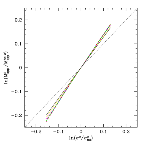
FIG. 12.: Relation between the aperture mass variance and the overall normalization of the matter power spectrum ($\sigma^{2}$). Both values are normalized to the values for the fiducial model. Clockwise, the curves correspond to $\theta=$10, 15, 20, 25, 33, 42 and 50 respectively. Our approximation that these curves are straight lines is seen to be quite accurate. Their slope approaches unity (dotted line) in the linear regime (for very large $\theta$).

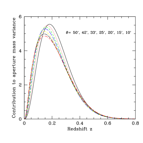
FIG. 13.: Curves show ${\cal P}^{\rm z}(z)$ normalized to have unit area. These curves show where the contribution to the aperture mass originates in redshift for each of the seven values of $\theta$ from [9].

C Cluster data

The abundance of galaxy clusters at various redshifts is emerging as an increasingly powerful probe of cosmological parameters, as new surveys are enlarging cluster samples and x-ray, SZ, optical and lensing observations of cluster properties are improving our understanding of the underlying physics.

In principle, a suite of hydrodynamical simulations including all the relevant physics could be used to map out the region in cosmological parameter space that matched the observed cluster abundance. In practice, this is still not numerically feasible, so published constraints involve a series of approximations. At a minimum, this tends to involve the Press-Schechter approximation or variations thereof [49, 50, 51] to predict the mass function of dark halos and some way of inferring the mass of the dark halo from the observed properties of the cluster. For example, in studies using X-rays, a mass-temperature relation that connects the halo mass with an observed cluster x-ray temperature is needed. The consensus result is that cluster data constrains mainly a combination of the normalization of the power spectrum on the cluster scale and the cosmic density parameter $\Omega_{\rm m}$. The normalization is usually quoted as the rms density fluctuation $\sigma(R)$ in a sphere of radius $R=8h^{-1}$Mpc, given by

$$\sigma_{R}^{2}\equiv{4\pi\over(2\pi)^{3}}\int_{-\infty}^{\infty}\left[{3j_{1}(kR)\over(kR)}\right]^{2}k^{3}P(k)d\ln k,$$ (24)

where the 1st spherical Bessel function is $j_{1}(x)=(\sin x-x\cos x)/x^{2}$.

For instance, a recent SDSS analysis reports $\sigma_{8}=(0.35\pm 0.03)\Omega_{\rm m}^{-0.60}$ [52], basing cluster mass estimates on richness rather than x-ray. However, it has been argued [53] that quoting results using $R=8h^{-1}$Mpc is confusing, since the cluster abundance is mainly sensitive to slightly larger scales centered around $R\sim 15h^{-1}$Mpc. The $\Omega_{\rm m}$-dependence above comes mainly from the fact that the mean density $\Omega_{m}$ enters in the Press-Schechter formula and collapse overdensity approximation, but also from a small $\Omega_{\rm m}$-dependent correction for evolution between $z=0$ and the redshifts observed (say $z=0.1-0.2$). Including the additional $\Omega_{\rm m}$-dependence coming from the fact that $\Omega_{\rm m}$ affects the shape of the power spectrum and hence the ratio ratio $\sigma_{15}/\sigma_{8}$, a result like $\sigma_{8}\propto\Omega_{\rm m}^{-0.6}$ changes significantly, to something like $\sigma_{8}\propto\Omega_{\rm m}^{-0.2}$ [53].

Since we wish to plot constraints on the power spectrum $P(k)$ of the form of equation (1), we follow [53] and use the normalization $\sigma_{R}$ at $R=9\Omega_{m}^{-0.41}\approx 15h^{-1}$Mpc. This scale corresponds to a 6.5keV cluster forming now, and has the property of giving constraints that to first approximation depend on $P(k)$ only via its normalization ($\sigma_{R}$), not via its shape [53]. Using our convention $(\star)$ to plot the $k$-range probed by clusters, the 20th, 50th and 80th percentiles of the integrand in equation (24) fall at $k\approx$0.06, 0.10 and 0.15$h/$Mpc, respectively.

Table 2 gives a recent sample of cluster measurements of the power spectrum normalization, all quoted for $\Omega_{\rm m}=0.3$ for comparison. We see that although the quoted error bars are as small as 0.05-0.08, the spread in $\sigma_{8}$ between papers is many times larger, as great as $0.41$ even during the past year. Since this suggests that systematic uncertainties are still larger than statistical uncertainties, we simply use the constraint $\sigma_{8}=0.8\pm 0.2$ to be conservative, mapped to $R=15h^{-1}{\rm Mpc}$ as in [53] to reduce power spectrum shape dependence.

Table 2 – Recent measurements of the $P(k)$ normalization using cluster abundances.

Analysis		$\sigma_{8}$
Pierpaoli et al. (2001)	[53]	$1.02^{+0.07}_{-0.08}$
Borgani et al. (2001)	[54]	$0.76^{+0.08}_{-0.05}$
Reiprich & Böhringer (2001)	[55]	$0.68^{+0.08}_{-0.06}$
Seljak et al. (2001)	[56]	$0.75\pm 0.06$
Viana et al. (2001)	[57]	$0.61\pm 0.05$
Bahcall et al. (2002)	[52]	$0.72\pm 0.06$

D Ly$\alpha$ Forest data

The Lyman $\alpha$ forest (Ly$\alpha$F) is the plethora of absorption lines in the spectra of distant quasars caused by neutral hydrogen in overdense intergalactic gas along the line of sight. By tracing the cosmic gas distribution out to great distances, it offers a new and exciting probe of matter clustering on even smaller scales than currently accessible to CMB and weak lensing, when the universe was merely 10-20% of its present age. Since the gas probed by the Ly$\alpha$F is only overdense by a modest factor relative to the cosmic mean, the hope is that all the relevant physics can be simulated, thereby connecting the observations to the underlying matter power spectrum [58, 59, 60, 61, 62].

The most ambitious such analysis to date [11] claimed to do just this, measuring $P(k)$ on 13 separate scales $k$ using 53 quasar spectra. An extensive reanalysis by an independent group [10] has suggested that the technique basically works. One should keep in mind that there are many caveats to the Lyman $\alpha$ forest analysis. One wonders to what extent all the relevant physics is included in the hydro-simulations and the dark-matter-only prescriptions that have been developed and how the uncertainties in the reionization history, the ionizing background and its fluctuations propagate into the reconstruction of $P(k)$. Moreover, even for the evolution of the dark matter alone, which is the basis of the simple Ansatz used to determine $P(k)$ from the Ly$\alpha$F data, non-linear corrections significantly affect the evolution of clustering on the scales relevant for the Ly$\alpha$F because the slope of the $P(k)$ around the non-linear scale is much closer to $n_{eff}=-3$ than it is today [63]. We should view the reconstructed points as an inversion done assuming that all the relevant physics was correctly modeled and that the departures from the fiducial model (which in this case also involve other details such as the reionization history) are sufficiently small.

Figure 1 shows the reanalyzed data [10] with the quoted statistical and “systematic” errors added in quadrature. The plotted errors do not include an overall multiplicative error of $17\%$ stemming from temperature and optical depth uncertainties, and the mapping from the observation redshift $z\sim 2.72$ to today may introduces additional horizontal and vertical shifts that depend on $\Omega_{\rm m}$ and $\Omega_{\Lambda}$ as described in Section III. We use the approximation of [10] that the window functions are Gaussian with width $\Delta k\approx 25\ {\rm km/s}\ (k\times{\rm km/s})^{-1/2}$. The 13th point is a mere upper limit, omitted to avoid clutter.

E Galaxy clustering data

Two- and three-dimensional maps of the Universe provided by galaxy redshift surveys constitute the $P(k)$ probe with the longest tradition. Indeed, the desire to measure $P(k)$ was one of the prime motivations behind ever more ambitious observational efforts such as the the CfA/UZC [64, 65], LCRS [66] and PSCz [67] surveys, each well in excess of $10^{4}$ galaxies. The most accurate power spectrum measurement to date is from the 2 Degree Field Galaxy Redshift Survey (2dFGRS) [17], soon to be overtaken by the Sloan Digital Sky Survey (SDSS) [18] which aims for 1 million galaxies.

Band powers measured from galaxy surveys are related to the underlying matter power spectrum by

$$d_{i}=\int_{-\infty}^{\infty}W_{i}(k)b(k)^{2}P(k)d\ln k,$$ (25)

where the window functions $W_{i}$ depend only on the geometry of the survey and the method used to analyze it. Here $b(k)$ is the bias, reflecting the fact that galaxies need not cluster the same way as the underlying matter distribution, and defined simply as the square root of the ratio of galaxy power to matter power. Figure 1 shows the 2dFGRS power spectrum as measured with the PKL eigenmode technique [8], which has the advantage of producing uncorrelated error bars and narrow, exactly computable window functions $W_{i}$ (see also [68]).

With galaxy clustering measurements, bias is the key caveat. On small-scales, bias is known to be complicated, with the galaxy power spectrum saying more about the galaxy distribution within individual dark matter halos than about the underlying matter distribution. We have therefore plotted 2dFGRS measurements only for $k<0.3h/{\rm Mpc}$. Fortunately, a broad class of bias models predict that $b(k)$ should be simple and independent of $k$ on large scales [69, 70, 71, 72, 73]. Even if this is true, however, the measured large-scale 2dFGRS power spectrum is likely to have slightly scale-dependent bias, masquerading as evidence for a redder power spectrum, i.e., one with a smaller spectral index $n$. This is because the power spectrum is measured from a heterogeneous magnitude-limited sample mixing galaxies of very different kinds. Most of the information about $P(k)$ on large scales comes from distant parts of the survey, where bright ellipticals are over-represented since dimmer galaxies get excluded by the faint magnitude limit. Since more luminous galaxies are known to be more highly biased [74, 75], this should cause the bias to rise as $k\to 0$. With a massive data set like the SDSS, it will be possible to accurately measure how bias depends on luminosity and correct for this effect.

III Breaking the degeneracy between primordial power and transfer functions

Above we have shown how to map CMB, lensing, cluster and Ly$\alpha$F measurements into $k$-space when the transfer functions are known. These transfer functions depend on various Late Universe cosmological parameters (the reionization optical depth $\tau$ and the matter budget). To measure the Late Universe properties (these parameters) and the Early Universe properties (the primordial power spectrum $P_{*}(k)$) independently, we must therefore break the degeneracy between the two. This may at first sight appear hopeless, since the measurements involve products of primordial power and transfer functions, and there is no unique way of factoring a product into two terms. As will be described below, the problem can nonetheless be solved thanks to two separate facts in combination:

1. $\tau$ and the matter budget parameters affect different types of measurements in different ways.

2. There is substantial overlap in $k$-space between different types of measurements.

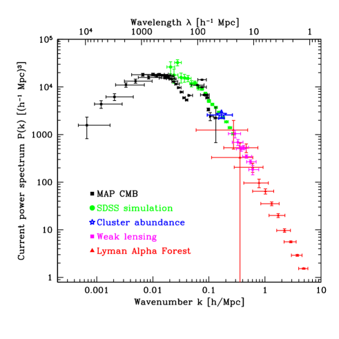
FIG. 14.: Same as Figure 9, but assuming a baryon density $h^{2}\Omega_{b}=0.07$ when analyzing the data. Since this figure makes no assumptions about the primordial power spectrum $P_{*}(k)$, the glaring discrepancy seen between the power spectrum inferred from CMB and galaxy clustering means that this high baryon fraction can be ruled out without assumptions about Early Universe physics.

A picture can say more than a thousand words, and both of these facts are illustrated by the example in Figure 14. It shows simulated data assuming that the concordance model of [5] is true, with the CMB mapped into $k$-space assuming a higher baryon density, $h^{2}\Omega_{b}=0.07$. This alters the CMB and matter transfer functions in quite different ways (details below), producing a strikingly wiggly $P(k)$ inferred from the CMB. Since MAP and SDSS overlap by over a decade in $k$ where this wiggliness is seen, it is obvious that the two are inconsistent and that such a high baryon density is ruled out. This conclusion can be drawn without assumptions about the primordial power spectrum $P_{*}(k)$, since this figure was generated without involving $P_{*}(k)$, merely using measurements and transfer function parameters.

In the next subsection, we will briefly discuss how the various types of measurements are affected by the Late Universe parameters and the relevance of this for measuring these parameters independently of $P_{*}(k)$. We then describe how how a “chi-by-eye” comparison as in Figure 14 can be replaced by a rigorous statistical method useful for cosmological parameter estimation.

A How Late Universe parameters affect the $P(k)$ recovered from different data sets

Although reconstruction of $P(k)$ as in Figure 14 has the advantage of minimizing the amount of processing applied to large-scale-structure (galaxy, lensing, cluster, Ly$\alpha$F) data the reconstructed primordial power $P_{*}(k)$ provides better intuition for the present discussion, since each data set has, loosely speaking, been divided by its own transfer function. In contrast, the CMB data in Figure 14 was (apart from smoothing effects) both divided by the CMB transfer function $W_{\l}(k)$ and multiplied by the matter transfer function $T(k)^{2}$. We will therefore center our discussion around $P_{*}(k)$ rather than $P(k)$ in the remainder of the paper.

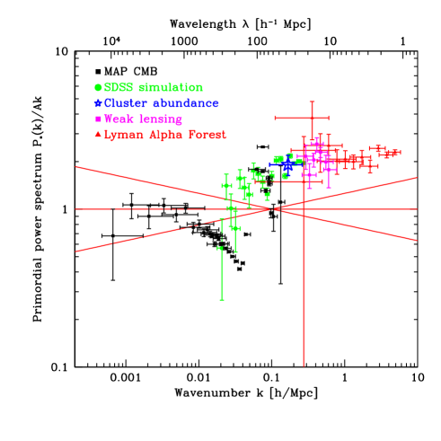
FIG. 15.: Same as Figure 8, but assuming a baryon density $h^{2}\Omega_{b}=0.07$ — a ruled out model.

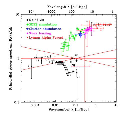
FIG. 16.: Same as Figure 8, but assuming a dark matter density $h^{2}\Omega_{c}=0.5$ — a ruled out model.

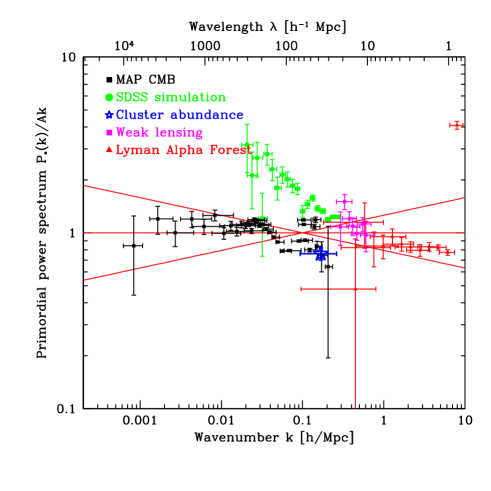
FIG. 17.: Same as Figure 8, but assuming a cosmological constant $\Omega_{\Lambda}=0.2$ — a ruled out model.

Imagine generating large numbers of plots like Figure 7, each one assuming different values for the Late Universe parameters to analyze the same measured data. Figure 15 shows the result for the above-mentioned case of a high baryon fraction, and is simply the $P_{*}$-version of Figure 14. Figures 16 and 17 show corresponding examples with incorrect assumptions for the cold dark matter density $h^{2}\Omega_{\rm cdm}$ and the cosmological constant $\Omega_{\Lambda}$. Before delving into details, a few basic facts should be noted. The LSS (cluster, lensing, Ly$\alpha$F and galaxy) points tend to shift together, since they are all sensitive to the matter transfer function $T(k)^{2}$. These LSS points split apart when certain parameters are altered, however, notably $\Omega_{\rm m}$ and the cosmic expansion history $a(t)$, which affect the four differently. In contrast, the CMB points separate from the other four data types whenever any Late Universe parameter is changed, indeed often by shifting in a rather opposite direction from the others.

The recent literature on cosmological model constraints includes a bewilderingly large list of cosmological parameters:

$${\bf p}\equiv(\tau,\Omega_{\rm k},\Omega_{\Lambda},\Omega_{x},w,\omega_{\rm dm},\omega_{\rm b},f_{\nu},A_{s},n_{s},\alpha,A_{t},n_{t}).$$ (26)

These are the reionization optical depth $\tau$, the primordial amplitudes $A_{s}$, $A_{t}$ and tilts $n_{s}$, $n_{t}$ of scalar and tensor fluctuations, the running of the scalar tilt $\alpha$, and seven parameters specifying the cosmic matter budget. The various contributions $\Omega_{i}$ to critical density are for curvature $\Omega_{\rm k}$, vacuum energy $\Omega_{\Lambda}$, other dark energy $\Omega_{x}$ (with an equation of state $w$), cold dark matter $\Omega_{\rm cdm}$, hot dark matter (neutrinos) $\Omega_{\nu}$ and baryons $\Omega_{\rm b}$. The quantities $\omega_{\rm b}\equiv h^{2}\Omega_{\rm b}$ and $\omega_{\rm cdm}\equiv h^{2}\Omega_{\rm dm}$ correspond to the physical densities of baryons and total (cold + hot) dark matter ($\Omega_{\rm dm}\equiv\Omega_{\rm cdm}+\Omega_{\nu}$), and $f_{\nu}\equiv\Omega_{\nu}/\Omega_{\rm dm}$ is the fraction of the dark matter that is hot. Additional parameters that are often mentioned are not independent, for instance the total matter density $\Omega_{\rm m}\equiv\Omega_{\rm b}+\Omega_{\rm dm}$ and the dimensionless Hubble parameter $h\equiv\sqrt{(\omega_{\rm cdm}+\omega_{\rm b})/(1-\Omega_{\Lambda}\Omega_{\rm k})}$.

Fortunately, the underlying physics is simpler than this parameter profusion suggests. $A_{s}$, $n_{s}$ and $\alpha$ are merely a particular parametrization of the primordial power spectrum, corresponding to the Ansatz $P_{*}(k)=A_{s}k^{n_{s}+\alpha\ln k}$. $A_{t}$ and $n_{t}$ similarly parametrize the primordial tensor (gravity wave) power spectrum as a power law. In other words, only the first eight parameters in equation (26) are Late Universe parameters affecting the transfer functions — we refer to all of these except $\tau$ as the matter budget parameters. The tensor parameters $A_{t}$ and $n_{t}$ are of only marginal relevance to this paper, since they affect only the CMB and do so essentially only on scales larger than those that overlap with large-scale-structure observations. This means that if we assume $A_{t}>0$ in our reconstruction, the CMB measurements of $P_{*}(k)$ would shift downwards in Figure 15, but only to the left where they cannot be compared with other data. Since our method for measuring Late Universe parameters involves comparing CMB with LSS data, it is therefore essentially unaffected by tensor fluctuations.

A similar simplification applies to $\tau$, which also affects only the CMB. On the small scales where the CMB overlaps with other measurements, the effect of reionization in merely to suppress the CMB power spectrum by a constant factor $e^{2\tau}$.

A further simplification is that $\Omega_{\Lambda}$, $\Omega_{x}$ and $w$ never enter in any other way than as a particular parametrization of the cosmic expansion history $a(t)$ or, equivalently, of the function

$${H(z)\over H_{0}}=\left[(1+z)^{3}\Omega_{\rm m}+(1+z)^{2}\Omega_{\rm k}+(1+z)^{3(1+w)}+\Omega_{\Lambda}\right],$$ (27)

where the Hubble parameter $H\equiv d\ln a/dt$. Various integrals involving this function determine the growth of linear clustering, the brightness and angular size of distant objects, and volume-related effects. This function causes merely a sideways shift in the CMB on the scales that LSS can probe, since the late ISW effect is important only on larger scales. Beyond the parameters in this function, the only remaining matter budget parameters are thus $\omega_{\rm m}$, $\omega_{\rm b}$, $f_{\nu}$, specifying the physical densities of cold dark matter, baryons and neutrinos, respectively.

Detailed discussions how the CMB and matter transfer functions depend on cosmological parameters can be found in, e.g., [76, 77, 78]. For the reader interested in more empirical intuition, the movies at $www.hep.upenn.edu/{\sim}max/cmb/movies.html$ are recommended. The key point about to take away from all this is that the CMB and matter transfer functions depend quite differently on the matter budget parameters, often in rather opposite ways. For instance, increasing the cold dark matter density $\omega_{\rm cdm}$ shifts the galaxy power spectrum up to the right and the CMB peaks down to the left. Adding more baryons boosts the odd-numbered CMB peaks but suppresses the galaxy power spectrum rightward of its peak and also makes it wigglier. Increasing the dark matter percentage that is hot (neutrinos) suppresses small-scale galaxy power while leaving the CMB almost unchanged. (The recovered points in our $P_{*}(k)$ figures always respond in the sense opposite to that in these movies when assumed parameters are varied.) This means that combining CMB with LSS data allows unambiguous determination of the matter budget.

Since the heights of the CMB peaks are controlled by the densities of ordinary ($\omega_{\rm b}$) and dark ($\omega_{\rm dm}$) matter, assuming the wrong values for these parameters is seen to results in a wiggly $P_{*}(k)$ from CMB in Figures 15 and 16. Increasing $\omega_{\rm b}$ boosts predominantly the odd-numbered CMB peaks whereas increasing $\omega_{\rm cdm}$ suppresses the CMB peaks with less of an even/odd asymmetry as well as shifting the peaks to the left, so the CMB points in these figures are seen to depart from unity in the opposite sense. Increasing the baryon fraction $\omega_{\rm b}/\omega_{\rm dm}$ produces larger wiggles in the matter power spectrum as well, together with an overall power suppression leftward of the peak. Increasing the dark matter density $\omega_{\rm dm}$ pushes the turnover in $P(k)$, corresponding to the horizon size at the matter-radiation equality epoch, to the right and thereby boosts small-scale power. There is also a sideways shift in both CMB and matter clustering, since the $h$ on the horizontal axis changes with the matter budget parameters. $H(z)$ gives shifts the transfer functions vertically via the linear growth factor and horizontally (angle-diameter distance changes, and well as the $h$ in the horizontal axis definition). Here is a brief summary of how the curves $P_{*}(k)$ recovered from CMB and LSS measurements get affected when the assumed parameters are changed:

• $\omega_{\rm b}$, $\omega_{\rm cdm}$: cause wiggles

• $f_{\nu}$: boosts LSS points on small scales

• $\Omega_{\rm k}$, dark energy: cause wiggles via incorrect CMB peak locations, vertical offset

• $\tau$: boosts CMB points by $e^{2\tau}$ where they overlap with LSS

Some parameters also affect the conversion of observed LSS data to measurements of $P(k)$ as illustrated in Figure 17. The cluster point scales roughly as $\Omega_{\rm m}^{-1.2}$ in power ($\Omega_{\rm m}^{-0.6}$ in amplitude), mainly because $\Omega_{\rm m}$ enters in the Press-Schechter prescription for halo abundance and in the approximation for collapse overdensity. For weak lensing, a factor of $\Omega_{\rm m}^{2}$ enters in the definition of the cosmic shear power spectrum, although the final scaling with $\Omega_{\rm m}$ is complicated by nonlinearities. All four LSS observables at $z>0$ must be mapped to $z=0$, which involves a vertical shift due to clustering growth and a horizontal shift from the computation of comoving length scales, and these shifts are both given by the cosmic expansion history $H(z)$ of equation (27). Since these shifts increase with $z$, they are most important for the Ly$\alpha$F. Finally, the $P(k)$ reconstruction from galaxies, clusters and the Ly$\alpha$F depend at least weakly on the baryon fraction $\Omega_{\rm b}/\Omega_{\rm m}$, as is evident from considering what entities like galaxy bias, the cluster temperature function would be like in the limit of zero baryons.

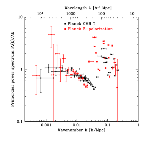
FIG. 18.: Simulation of the primordial power spectrum recovered from the upcoming Planck CMB satelle using unpolarized and polarized data, assuming a baryon density $h^{2}\Omega_{b}=0.07$ — a ruled out model. Note that the bias goes in opposite directions, since polarized and unpolarized peaks are out of phase. The simulation was performed using all Planck channels and the MID foreground model from [33].

CMB polarization provides another powerful and independent tool for breaking the degeneracy between Early and Late Universe parameters. The key reason for this is that the polarized acoustic peaks are out of phase with the unpolarized ones, with the peaks in the E power spectrum lining up with troughs in the unpolarized (T) power spectrum. This means that an incorrect assumed value for a parameter affecting peak heights (notably $\omega_{\rm b}$ and $\omega_{\rm cdm}$) causes the primordial power spectrum $P_{*}(k)$ recovered from T and E will to be biased in opposite directions. This useful fact is illustrated in Figure 18, which shows simulated measurements from the Planck satellite mapped into $k$-space. Note in particular the wiggle at $k\sim 0.04h/{\rm Mpc}$, where the T-points go low whereas the E-points go high, revealing that the high baryon fraction assumed is ruled out at high significance from CMB data alone, without any assumptions about the shape of the primordial power spectrum.

B Measuring Late Universe parameters independently of $P_{*}(k)$

Above we described the physics that makes it possible to break the degeneracy between Early Universe parameters ($P_{*}(k)$) and Late Universe parameters ($\tau$ and the matter budget). We now turn to the issue of how to do this in practice in a statistically rigorous way.

C The basic problem

Our basic problem is to measure a vector ${\bf p}$ of Late Universe parameters, say

$${\bf p}\equiv(\tau,\omega_{\rm dm},\omega_{\rm b},f_{\nu},\Omega_{\rm k},\Omega_{\Lambda}),$$ (28)

independently of $P_{*}(k)$. Our basic approach is to map all measurements into (linear) $k$-space and test if they are consistent with one another. Repeating this for a fine grid of models ${\bf p}$, we can map out the region of parameter space that is allowed, i.e., where the data are consistent.

To be specific, let us consider the case of comparing two types of data, for instance the MAP CMB power spectrum with the SDSS galaxy power spectrum. The challenge is that although they exhibit substantial overlap in scale, as seen in Figure 8, they generally have different window functions. This means that we cannot simply subtract the two independent measurements of $P_{*}(k)$ from each other and require the result to vanish — it would not vanish even in the absence of measurement errors, since the two experiments are probing different linear combinations of the underlying function $P_{*}(k)$.

Fortunately, a mathematically equivalent problem has already been extensively investigated in the literature, and we can employ the solution to test our data sets for consistency. The question of whether there is any power spectrum that is consistent with given band power measurements was studied in [79] for the case of two band powers and generalized to multiple ones in [80]. For $n$ band-powers, the best fit power spectrum was found to be a linear combination of up to $n-1$ delta-functions [80]. However, finding their locations is numerically time-consuming for large $n$, which motivated revisiting the problem. A fast general method was presented in [81] but was somewhat complicated, involving a series of eigenvalues computations. Finally, an information-theoretically optimal method was derived in [82] for different purposes (comparing CMB maps), which solves our present problem as well. This method has also been used to test CMB experiments for consistency [82, 4]. Since it is not only better (in terms of statistical rejection power) but also simpler than the above-mentioned alternatives, we will summarize it briefly below. It consists of two parts: “deconvolving” the effect of the window functions and testing the resulting two measurements for consistency. In summary, our method thus consists of the following three steps:

1. Map the measurements into $k$-space for fixed a ${\bf p}$

2. Deconvolve the effect of window functions

3. Test the deconvolved measurements for consistency

These three steps are repeated for a fine grid of ${\bf p}$-vectors to map out the allowed region in ${\bf p}$-space. The implementation of Step 1 was described in Section II and we now turn to Step 2 and Step 3.

1 Deconvolving the effect of window functions

Let us model the primordial power spectrum $P_{*}(k)$ as piecewise constant in a large number of narrow $k$-bins, with $x_{i}$ denoting the value of $P_{*}$ in the $i^{th}$ bin, and arrange the numbers $x_{i}$ into a vector ${\bf x}$. Grouping our two sets of band-power measurements into vectors ${\bf y}_{1}$ and ${\bf y}_{2}$, this means that they are related to ${\bf x}$ by

$${\bf y}_{1}={\bf W}_{1}{\bf x}+{\bf n}_{1},\quad{\bf y}_{2}={\bf W}_{2}{\bf x}+{\bf n}_{2},$$ (29)

for some known window matrices ${\bf W}$ that are simply discretized versions of the window functions computed in Section II and some noise vectors with known statistical properties. We assume that the measurements are unbiased so that $\langle{\bf n}_{i}\rangle={\bf 0}$ and define the noise covariance matrices

$${\bf N}_{1}\equiv\langle{\bf n}_{1}{\bf n}_{1}^{t}\rangle,\quad{\bf N}_{2}\equiv\langle{\bf n}_{2}{\bf n}_{2}^{t}\rangle,$$ (30)

In this subsection, we describe how the annoying ${\bf W}$-matrices can be eliminated by computing two deconvolved data sets ${\bf x}_{i}$, $i=1,2$, with the properties

$${\bf x}_{i}={\bf x}+{\bf n}^{\prime}_{i},\quad\langle{\bf n}^{\prime}_{i}\rangle={\bf 0},$$ (31)

and known covariance matrices ${\bf\Sigma}_{i}\equiv\langle{{\bf n}^{\prime}_{i}}{{\bf n}^{\prime}_{i}}^{t}\rangle$.

In the generic case, such deconvolution is strictly speaking impossible: we cannot compute ${\bf W}_{i}^{-1}{\bf y}_{i}$ since ${\bf W}_{i}$ is not invertible. Certain pieces of information about ${\bf x}$ are simply not present in ${\bf y}_{i}$, for instance about sharp features on scales much smaller than the widths of the window functions or about $k$-scales outside the region probed by the observations. The basic idea in Appendix D of [83] is to accept that certain modes in ${\bf x}$ cannot be recovered, and to record this information in the noise covariance matrix ${\bf\Sigma}_{i}$ for ${\bf x}_{i}$ by assigning a huge variance to these modes. Any subsequent analysis (in our case consistency testing) will then automatically assign essentially zero weight to these modes. This is useful in practice since all complications related to window functions are transferred from ${\bf W}_{i}$ to ${\bf\Sigma}_{i}$ where, as we will see in the next subsection, they are straightforward to deal with.

The method can be interpreted as combining the real data ${\bf y}_{i}$ with data from a virtual experiment that is so noisy that it contains essentially no information, yet has enough information to remove all numerical singularities by providing independent measurements of each $x_{i}$ with some huge standard deviation $\sigma$. The final result is [83]

$${\bf x}_{i} = {\bf\Sigma}_{i}{\bf W}_{i}^{t}{\bf N}_{i}^{-1}{\bf y}_{i},$$ (32)

$${\bf\Sigma}_{i} = \left[{\bf W}_{i}^{t}{\bf N}_{i}^{-1}{\bf W}_{i}+\sigma^{-2}{\bf I}\right]^{-1}.$$ (33)

One finds [83] that this prescription has all desired properties as long as $\sigma$ is chosen to be a few orders of magnitude larger than the error bars in the real data, and it also has the property of minimizing the noise variance in the deconvolved data. If we were to choose $\sigma$ to be too small, then the virtual experiment would contribute a non-negligible amount of information and bias the results. If we were to choose $\sigma$ to be too large, however, the matrix ${\bf\Sigma}_{i}$ would contain some enormous eigenvalues (since ${\bf W}_{i}^{t}{\bf\Sigma}_{i}^{-1}{\bf W}_{i}$ is typically not invertible) and be poorly conditioned, causing numerical problems.

2 Testing the deconvolved measurements for consistency

To make explicit that our mapping of measurements into $k$-space depends on the assumed Late Universe parameters ${\bf p}$, we will denote the deconvolved measurements and their noise covariance matrices ${\bf x}_{i}({\bf p})$ and ${\bf\Sigma}_{i}({\bf p})$ from now on $(i=1,2)$. Given these two deconvolved measurements ${\bf x}_{1}({\bf p})$ and ${\bf x}_{2}({\bf p})$ of the primordial power spectrum vector ${\bf x}$ (from MAP and SDSS, say), we wish to test if they are consistent. If they are not, this rules out the Late Universe parameters ${\bf p}$ that were assumed to construct them.

Letting ${\bf z}$ denote the difference of the two power spectrum measurements,

$${\bf z}({\bf p})\equiv{\bf x}_{1}({\bf p})-{\bf x}_{2}({\bf p}),$$ (34)

we consider two hypotheses:

• The null hypothesis that the assumed Late Universe parameters ${\bf p}$ are correct. Then $\langle{\bf x}_{i}({\bf p})\rangle={\bf x}$, so that the difference spectrum ${\bf z}({\bf p})$ consists of pure noise with zero mean and covariance matrix ${\bf\Sigma}({\bf p})\equiv\langle{\bf z}({\bf p}){\bf z}({\bf p})^{t}\rangle={\bf\Sigma}_{1}({\bf p})+{\bf\Sigma}_{2}({\bf p})$.

• The alternative hypothesis that the assumed Late Universe parameter vector ${\bf p}$ is incorrect. In this case, ${\bf z}({\bf p})$ is expected to on average depart more from zero than under the hypothesis $H_{0}$, since both ${\bf x}_{1}({\bf p})$ and ${\bf x}_{2}$(p) become biased power spectrum measurements and typically get biased in quite different ways (Figures 15-17).

We will model $H_{1}$ as a change in the mean, $\langle{\bf z}\rangle={\bf m}\neq{\bf 0}$. It can be shown [81, 4] that the “null-buster” statistic

$$\nu({\bf p})\equiv\frac{{\bf z}({\bf p})^{t}{\bf\Sigma}({\bf p})^{-1}{\bf Q}{\bf\Sigma}({\bf p})^{-1}{\bf z}({\bf p})-\hbox{tr}\,\{{\bf\Sigma}({\bf p})^{-1}{\bf Q}\}}{\left[2\>\hbox{tr}\,\{{\bf\Sigma}({\bf p})^{-1}{\bf Q}{\bf\Sigma}({\bf p})^{-1}{\bf Q}\}\right]^{1/2}}$$ (35)

rules out the null hypothesis $H_{0}$ with the largest average significance $\langle\nu\rangle$ if $H_{1}$ is true provided one chooses ${\bf Q}={\bf m}{\bf m}^{t}$. The statistic can be interpreted as the number of “sigmas” at which $H_{0}$ is ruled out [81]. Note that for the special case ${\bf Q}\propto{\bf\Sigma}({\bf p})$, it simply reduces to $\nu=(\chi^{2}-n)/\sqrt{2n}$, where $\chi^{2}\equiv{\bf z}^{t}{\bf\Sigma}({\bf p})^{-1}{\bf z}$ is the standard chi-squared statistic. The null-buster test can therefore be viewed as a generalized $\chi^{2}$-test which places more weight on those particular modes where the expected signal-to-noise is high. It has proven successful comparing both CMB maps [83, 84, 82], galaxy distributions [85, 86] and CMB power spectra [4]. Tips for rapid implementation in practice are given in [83].

Any choice of ${\bf Q}$ results in a statistically valid test: for instance, the region in the Late Universe parameter space for which $\nu({\bf p})>2$ is ruled out at the $2-\sigma$ level. This corresponds to 97.5% significance with the usual frequentist interpretation as a one-sided test if there are many similarly large eigenvalues of ${\bf\Sigma}^{-1/2}{\bf Q}{\bf\Sigma}^{-1/2}$, since it makes the generalized $\chi^{2}$ distribution of $\nu$ approximately Gaussian by the central limit theorem.

What is the best choice of ${\bf Q}$? The above-mentioned choice ${\bf Q}={\bf m}{\bf m}^{t}$ placed all weight on a single mode ${\bf m}$. More generally, the test pays the greatest attention to those eigenvectors of ${\bf Q}$ whose eigenvalues are large. The standard $\chi^{2}$-test (the choice ${\bf Q}={\bf\Sigma}$) has the attractive feature of giving an assumption-free consistency test: since ${\bf Q}$ has no vanishing eigenvalues, it is sensitive to any type of discrepancies between the two power spectrum measurements ${\bf x}_{1}({\bf p})$ and ${\bf x}_{2}({\bf p})$.

If the goal is to place sharp constraints on cosmological parameters, however, the statistical rejection power of the test can be boosted by placing the statistical weight on precisely those types of departures which correspond to incorrect parameter assumptions. If the rms uncertainties on the parameters $p_{i}$ can be estimated using the Fisher matrix [87] ${\bf F}_{ij}={\partial{\bf m}^{t}/\partial p_{i}}{\bf\Sigma}^{-1}{\partial{\bf m}/\partial p_{j}}$ (with $i$ and $j$ running over the parameters), the choice

$${\bf Q}\equiv\sum_{ij}({\bf F}^{-1})_{ij}{\partial{\bf m}\over\partial p_{i}}{\partial{\bf m}^{t}\over\partial p_{j}}$$ (36)

will have this attractive property as long as the ${\bf p}$-vectors considered are fairly close to the true value — a desirable situation that the cosmology community will hopefully keep approaching as data keeps improving.

Indeed, in this high signal-to-noise limit, the nullbuster test with the weighting given by equation (36) can be thought of as the frequentist analog of a Bayesian likelihood analysis. To understand this we can calculate the expectation value of $\nu$ assuming $H_{1}$ is true to lowest order in the parameter differences $\Delta p_{i}$. To do so we take the expectation value of equation (35), use $\langle{\bf z}{\bf z}^{t}\rangle={\bf\Sigma}+{\bf m}{\bf m}^{t}$ and ${\bf m}\approx({\partial{\bf m}^{t}/\partial p_{i}})\Delta p_{i}$ and get,

$$\langle\nu\rangle\approx{\Delta{\bf p}^{t}{\bf F}{\Delta\bf p}\over\sqrt{2N_{p}}},$$ (37)

where $N_{p}$ is the number of parameters. We can compare this result to what would be obtained using a likelihood analysis. In the Gaussian approximation, the likelihood of the null hypothesis is given by

$$\L\propto|{\bf\Sigma}|^{-1/2}e^{-{1\over 2}{\bf z}^{t}{\bf\Sigma}^{-1}{\bf z}}.$$ (38)

Thus if we calculate the expected value of the logarithm of this likelihood assuming again that $H_{1}$ is true (again to lowest order in $\Delta{\bf p}$) we get

$$\langle\ln\L\rangle\approx-{1\over 2}{\Delta\bf p}^{t}{\bf F}{\Delta\bf p}$$ (39)

up to an irrelevant additive constant, the usual result that the Fisher matrix gives the curvature of the log-likelihood around the maximum. This shows that on average and to lowest order in $\Delta{\bf p}$, the (frequentist) nullbuster statistic coincides with the log-likelihood that one would calculate in a Baysian framework, and so on average one would rule out the same region of parameter space with both methods.

Note that although it is tempting to perform a standard Bayesian likelihood analysis using a “likelihood” similar to equation (38), it is not obvious that this can be given the standard interpretation in terms of Bayes’ theorem, since it is not only $\langle{\bf z}\rangle$ and ${\bf\Sigma}$ that depend on ${\bf p}$ (as usual), but also the data itself: ${\bf z}={\bf z}({\bf p})$. Since there are no such interpretational issues with the frequentist null-buster test, it is therefore reassuring that the two approaches approximately agree.

D Further applications

Above we described how requiring consistency between two sets of measurements (say MAP and SDSS) could constrain the Late Universe parameters without assumptions about the primordial power spectrum $P_{*}(k)$. Given three or more types of data, an obvious extension is to first test two for consistency (say lensing and Ly$\alpha$F), then for the parameter subspace where they are consistent, combine them as in [81] and test the result against a third type of data. Since the LSS data share many parameter dependencies as discussed in Section III A, it is natural to first let galaxy clustering, lensing, cluster and Ly$\alpha$F measurements slug it out amongst themselves and then compare the resulting spectrum combining all LSS data with CMB.

Once ${\bf p}$ has been constrained as described above, it becomes possible to measure $P_{*}(k)$ without assumptions about ${\bf p}$ for the very first time. One way to do this is to measure $P_{*}(k)$ as in Figure 8 using the best fit ${\bf p}$-vector, and then quantify the error bars and their correlations by recomputing $P_{*}(k)$ for a grid of models ${\bf p}$ in the allowed region of the Late Universe parameter space, effectively marginalizing over ${\bf p}$ using the observed constraints as a prior.

IV Discussion

We have presented a method which complements the traditional “black box” likelihood approach to cosmological parameter estimation in two ways: by testing underlying physical assumptions and by improving physical intuition for where the constraints come from. We described how CMB, galaxy, lensing, cluster and Ly$\alpha$F could be compared directly in (linear) $k$-space in Section II, then showed how a graphical chi-by-eye test could be transformed into a statistically rigorous method in Section III, providing independent measurements of Early Universe parameters (the primordial power spectrum $P_{*}(k)$) and Late Universe parameters ($\tau$ and the matter budget). We found that requiring consistency between unpolarized CMB measurements and either polarized CMB or large-scale structure data is quite promising in this regard.

Separating Early and Late Universe physics is particularly timely given the excess in the small-scale CMB power spectrum recently reported by the CBI team [88]. We have seen that the angular scales where this excess is seen correspond to spatial scales around $k\sim 0.2h/{\rm Mpc}$ where the power spectrum is already constrained by galaxy, lensing and cluster observations. This makes it difficult to blame the excess on the Early Universe, say by tilting or adding a feature in $P_{*}(k)$. The alternative explanation in terms of contamination from discrete SZ-sources has been shown to be extremely sensitive to the power spectrum normalization on the cluster scale, tentatively requiring $\sigma_{8}\approx 1$ [89]. With our convention $(\star)$, $\sigma_{8}^{2}$ probes the range $k\approx 0.17^{+0.09}_{-0.08}$, which according to Figure 5 corresponds approximately to the multipole range $\l=2000\pm 800$ if the concordance model [5] is not too far from the truth. The cluster normalization $\sigma_{R}^{2}$ with $R\approx 15h^{-1}{\rm Mpc}$ corresponds to $\l\approx 1100^{+600}_{-500}$, scales already probed by the shallower (mosaic) CBI observations [16]. The concordance model [5] normalized to the CMB data gives $\sigma_{8}=0.81$ assuming $\tau=0.05$, and it appears likely that quite accurate and robust $\sigma_{8}$-measurements based on the CMB normalization will be available down the road.

This paper is not intended to the final word on testing physical assumptions in cosmology, merely a small step to be followed by many more. In this spirit, let us close by summarizing some of the most important things that we have not done and some promising directions for future work.

An obvious first step is implementing our method to independently measure the Early and Late Universe parameters. Next year will be an appropriate time to do this, taking advantage of the revolutionary precision that will be offered by MAP. Since this will involve working with a large grid of CMB transfer functions, the approximations described in [90] will be useful for this.

We have made one important assumption throughout this paper that it would desirable to test: that the primordial fluctuations are adiabatic. The adiabatic assumption means that the process generating the fluctuations in the Early Universe created density fluctuations without altering the density ratios of different matter components (photons, baryons, neutrinos, dark matter, etc.). By tinkering with these relative densities, it is possible to generate a variety of so-called isocurvature fluctuations. In addition to the familiar baryonic and CDM isocurvature modes, there are obscure ones, for instance a neutrino isocurvature mode where the ratio of neutrinos to photons varies spatially but the net density perturbation vanishes, and it can be shown that the most general case corresponds to a function $P_{*}(k)$ that is not a scalar but a $5\times 5$ symmetric matrix [91]. Although it has been shown that CMB polarization will help constrain isocurvature modes, real progress in this endeavor is likely to be some way off, requiring the sensitivity of the Planck satellite [93, 92, 94]. On the bright side, these complications matter only when studying CMB data, so it is valid to compare and combine the power spectra measured with galaxies, Ly$\alpha$F, lensing and clusters at low ($z\mathrel{\hbox to0.0pt{\lower 3.0pt\hbox{$\mathchar 536\relax$}\hss}\raise 2.0pt\hbox{$\mathchar 316\relax$}}10$, say) redshift as described above assuming purely adiabatic fluctuations.

Staying on the topic of still more general tests, there exist an elegant “generalized dark matter” formalism for describing the gravitational effects of the most general matter budget [95], and this is likely to place robust constraints on dark matter and dark energy as power spectrum measurements continue to accumulate over a range of redshifts.

Needless to say, CMB and LSS data will keep improving dramatically in coming years, providing greater sensitivity, $z$-range, $k$-range and $k$-resolution. In addition to the obvious advantages of sensitivity and range, galaxy window functions will become narrower as the SDSS sky coverage improves, improving the ability to detect sharp features in $P_{*}(k)$. For lensing, the shear power spectrum contribution from a given $z$ has delta function windows on $P(k)$ in the small-angle approximation, so the smearing in $k$-space comes from projection effects and can probably be substantially reduced using photometric redshift and topography techniques. For the Ly$\alpha$F, the $\sim 10^{5}$ SDSS quasar redshifts should greatly improve the measurement errors on larger spatial scales, where one may hope that uncertainties associated with nonlinear physics are smaller. In addition to the CMB and LSS probes we have utilized in this paper, many more appear promising. For instance, the recently claimed detection of galaxy halo substructure [96] falls right on our concordance curve in Figure 1 but two orders of magnitude further right than the other data points, at $k\sim 100{\rm Mpc}/h$. Searches for phase space clumpiness in the Milky Way halo with tidal streamers and future space-based astrometry may provide further constraints on dark matter clustering on such small scales, and additional clever observational ideas are undoubtedly waiting to be thought of. The SZ power spectrum is emerging as another promising cosmological observable, sensitive the $k$-range near the cluster scale [97].

This avalanche of precision data offers an exciting challenge to theorists in the community: to raise the ambition level to making precision cosmology mean more than merely more apocryphal decimal places, placing our understanding of the Universe on a solid foundation where the underlying physics has been tested rather than assumed.

The authors wish to thank Angélica de Oliveira-Costa, Arthur Kosowsky, Uros Seljak and David Spergel for helpful comments. This work was supported by NSF grants AST-0071213, AST-0134999, AST-0098606 and PHY-0116590, NASA grants NAG5-9194 & NAG5-11099, and two Fellowships from the David and Lucile Packard Foundation. MT is a Cottrell Scholar of Research Corporation.

REFERENCES

- [1] M. Tegmark, ApJL 514, L69 (1999).
- [2] M. Tegmark and M. Zaldarriaga, ApJ 544, 30 (2000).
- [3] M. Tegmark, M. Zaldarriaga, and A. J. S. Hamilton, PRD 63, 43007 (2001).
- [4] X. Wang, M. Tegmark, and M. Zaldarriaga, PRD 65, 123001 (2002).
- [5] G. Efstathiou et al., MNRAS 330L, 29 (2002).
- [6] A. Melchiorri and J. Silk, PRD 66, 041301R (2002).
- [7] A. Lewis and S. Bridle, astro-ph/0205436 (2002).
- [8] M. Tegmark, A. J. S. Hamilton, and Y. Xu, astro-ph/0111575 (2002).
- [9] H. Hoekstra, H. Yee, and M. Gladders, astro-ph/0204295 (2002).
- [10] N. Y. Gnedin and A. Hamilton J S, astro-ph/0111194 (2002).
- [11] R. A. C. Croft et al., astro-ph/0012324 (2000).
- [12] M. Tegmark, astro-ph/0101354 (2001).
- [13] M. Tegmark, Science 296, 1427 (2002).
- [14] Y. Wang and P. M. Garnavich, ApJ 552, 445 (2001).
- [15] D. Scott, J. Silk, and M. White, Science 268, 829 (1995).
- [16] T. J. Pearson et al., astro-ph/0205388 (2002).
- [17] M. Colless et al., MNRAS 328, 1039 (2001).
- [18] D. York et al., AJ 120, 1579 (2000).
- [19] A. R. Liddle and D. H. Lyth, Cosmological Inflation and Large-Scale Structure (Cambridge, Cambridge Univ. Press, 2000).
- [20] L. Amendola, S. Gottlöeber, J. P. Muecket, and V. Mueller, ApJ 451, 444 (1995).
- [21] R. Kates, V. Müller, S. Gottlöber, J. P. Mucket, and J. Retzlaff, MNRAS 277, 1254 (1995).
- [22] F. Atrio-Barandela, J. Einasto, S. Gottlöber, V. Müller, and A. A. Starobinsky, JETPL 66, 397 (1997).
- [23] J. Einasto, M. Einasto, E. Tago, A. A. Starobinsky, F. Atrio-Barandela, V. Müller, A. Knebe, and R. Cen, ApJ 519, 469 (1999).
- [24] Y. Wang, D. N. Spergel, and M. A. Strauss, ApJ 510, 20 (1999).
- [25] W. H. Kinney, PRD 63, 043001 (2001).
- [26] M. Matsumiya, M. Sasaki, and J. Yokoyama, PRD 65, 083007 (2002).
- [27] http://map.gsfc.nasa.gov
- [28] P. F. Scott et al., astro-ph/0205380 (2002).
- [29] E. Gawiser and J. Silk, Phys. Rept. 333-334, 245 (2000).
- [30] http://bubba.ucdavis.edu/knox/radpack.html
- [31] S. L. Bridle, Crittenden R, A. Melchiorri, M. P. Hobson, Kneissl R, and A. N. Lasenby, astro-ph/0112114 (2001).
- [32] U. Seljak and M. Zaldarriaga, ApJ 469, 437 (1996).
- [33] M. Tegmark, D. J. Eisenstein, W. Hu, and A. de Oliveira-Costa, ApJ 530, 133 (2000).
- [34] D. J. Eisenstein, astro-ph/0108153 (2001).
- [35] M. Bartelmann and P. Schneider, Phys. Rep. 340, 291 (2001).
- [36] H. Hoekstra, H. Yee, and Gladders M, astro-ph/0205205 (2002).
- [37] D. M. Wittman et al., Nature 405, 143 (2000).
- [38] L. Van Waerbeke et al., A&A 358, 30 (2000).
- [39] D. J. Bacon, A. R. Refregier, and R. S. Ellis, MNRAS 318, 625 (2000).
- [40] N. Kaiser, G. Wilson, and G. A. Luppino, astro-ph/0003338 (2000).
- [41] J. Rhodes, Refregier A, and E. J. Groth, astro-ph/0101213 (2001).
- [42] L. Van Waerbeke et al., astro-ph/0101511 (2001).
- [43] A. J. S. Hamilton, P. Kumar, E. Lu, and A. Matthews, ApJ 374, L1 (1991).
- [44] B. Jain, H. J. Mo, and S. D. M. White, MNRAS 276, L25 (1995).
- [45] J. A. Peacock and S. J. Dodds, MNRAS 280, 19 (1996).
- [46] A. Jenkins et al., Ap 499, 20 (1998).
- [47] A. Meiksin, M. White, and J. A. Peacock, MNRAS 304, 851 (1999).
- [48] B. Jain, U. Seljak, and S. White, ApJ 530, 547 (2000).
- [49] W. H. Press and P. Schechter, ApJ 187, 425 (1974).
- [50] R. K. Sheth, H. J. Mo, and G. Tormen, MNRAS 323, 1 (2001).
- [51] A. Jenkins et al., MNRAS 321, 372 (2001).
- [52] N. A. Bahcall, astro-ph/0205490 (2002).
- [53] E. Pierpaoli, D. Scott, and M. White, MNRAS 325, 77 (2001).
- [54] S. Borgani etal, ApJ 561, 13 (2001).
- [55] T. H. Reiprich and H. Boehringer, astro-ph/0111285 (2001).
- [56] U. Seljak, astro-ph/0111362 (2001).
- [57] P. T. P. Viana, R. C. Nichol, and A. R. Liddle, astro-ph/0111394 (2001).
- [58] V. K. Narayanan, D. N. Spergel, R. Davé, and C. P. Ma, ApJL 543, L103 (2000).
- [59] R. A. C. Croft, D. H. Weinberg, M. Pettini, L. Hernquist, and N. Katz, ApJ 520, 1 (1999).
- [60] M. White and R. A. C. Croft, ApJ 539, 497 (2000).
- [61] P. McDonald, J. Miralda-Escudé, M. Rauch, W. L. W. Sargent, T. A. Barlow, R. Cen, and J. P. Ostriker, ApJ 543, 1 (2000).
- [62] M. Zaldarriaga, L. Hui, and M. Tegmark, ApJ 557, 519 (2001).
- [63] M. Zaldarriaga, M. Scoccimarro, and L. Hui, astro-ph/0111230 (2001).
- [64] J. P. Huchra, M. J. Geller, V. de Lapparent, and II. G. Jr. Corwin, ApJS 72, 433 (1990).
- [65] E. E. Falco et al., PASP 111, 438 (1999).
- [66] S. A. Schectman et al., ApJ 470, 172 (1996).
- [67] W. Saunders et al., MNRAS 317, 55 (2000).
- [68] W. J. Percival et al., MNRAS 327, 1297 (2001).
- [69] P. Coles, MNRAS 262, 1065 (1993).
- [70] J. N. Fry and E. Gaztañaga, ApJ 413, 447 (1993).
- [71] R. J. Scherrer and D. H. Weinberg, ApJ 504, 607 (1998).
- [72] P. Coles, A. Melott, and D. Munshi, ApJ 521, 5 (1999).
- [73] A.. F. Heavens, S. Matarrese, and L. Verde, MNRAS 301, 797 (1999).
- [74] I. Zehavi et al., ApJ 571, 172 (2002).
- [75] P. Norberg et al., MNRAS 328, 64 (2001).
- [76] W. Hu, N. Sugiyama, and J. Silk, Nature 386, 37 (1997).
- [77] D. J. Eisenstein and W. Hu, ApJ 511, 5 (1999).
- [78] A. Kosowsky, M. Milosavljevic, and R. Jimenez, astro-ph/0206014 (2002).
- [79] R. Juszkiewicz, K. Górski, and J. Silk, ApJL 323, L1 (1987).
- [80] M. Tegmark, E. F. Bunn, and Hu W, ApJ 434, 1 (1994).
- [81] M. Tegmark, ApJ 519, 513 (1999).
- [82] Y. Xu, M. Tegmark, and A. de Oliveira-Costa, PRD 65, 083002 (2002).
- [83] Y. Xu, M. Tegmark, A. de Oliveira-Costa, M. Devlin, T. Herbig, A. D. Miller, C. B. Netterfield, and L. A. Page, PRD 63, 103002 (2001).
- [84] A. de Oliveira-Costa, M. Devlin, T. Herbig, A. D. Miller, C. B. Netterfield, L. A. Page, and M. Tegmark, ApJL 509, L77 (1998).
- [85] M. Tegmark and B. C. Bromley, ApJL 518, L69 (1999).
- [86] M. Seaborne et al., MNRAS 309, 89 (1999).
- [87] M. Tegmark, A. N. Taylor, and A. F. Heavens, ApJ 480, 22 (1997).
- [88] B. S. Mason, astro-ph/0205384 (2002).
- [89] J. R. Bond et al., astro-ph/0205386 (2002).
- [90] M. Kaplinghat, L. Knox, and C. Skordis, astro-ph/0203413 (2002).
- [91] M. Bucher, K. Moodley, and N. Turok, PRD 62, 083508 (2000).
- [92] M. Bucher, K. Moodley, and N. Turok, PRL 87, 191301 (2001).
- [93] K. Enqvist and H. Kurki-Suonio, PRD 61, 043002 (2000).
- [94] L. Amendola, C. Gordon, D. Wands, and M. Sasaki, PRL 88, 211302 (2002).
- [95] W. Hu, ApJ 506, 485 (1998).
- [96] N. Dalal and C. S. Kochanek, astro-ph/0202290 (2002).
- [97] U. Seljak, astro-ph/0205468 (2002).