Halo models of large scale structure

Abstract

We review the formalism and applications of the halo-based description of nonlinear gravitational clustering. In this approach, all mass is associated with virialized dark matter halos; models of the number and spatial distribution of the halos, and the distribution of dark matter within each halo, are used to provide estimates of how the statistical properties of large scale density and velocity fields evolve as a result of nonlinear gravitational clustering. We first describe the model, and demonstrate its accuracy by comparing its predictions with exact results from numerical simulations of nonlinear gravitational clustering. We then present several astrophysical applications of the halo model: these include models of the spatial distribution of galaxies, the nonlinear velocity, momentum and pressure fields, descriptions of weak gravitational lensing, and estimates of secondary contributions to temperature fluctuations in the cosmic microwave background.

1 Introduction

This review presents astrophysical applications of an approach which has its origins in papers by Jerzy Neyman & Elizabeth Scott and their collaborators nearly fifty years ago. Neyman & Scott [199] were interested in describing the spatial distribution of galaxies. They argued that it was useful to think of the galaxy distribution as being made up of distinct clusters with a range of sizes. Since galaxies are discrete objects, they described how to study statistical properties of a distribution of discrete points; the description required knowledge of the distribution of cluster sizes, the distribution of points around the cluster center, and a description of the clustering of the clusters [199]. At that time, none of these ingredients were known, and so in subsequent work [200, 201], they focussed on inferring these parameters from data which was just becoming useful for statistical studies.

Figure 1: The complex distribution of dark matter (a) found in numerical simulations can be easily replaced with a distribution of dark matter halos (b) with the mass function following that found in simulations and with a profile for dark matter within halos.

Since that time, it has become clear that much of the mass in the Universe is dark, and that this mass was initially rather smoothly distributed. Therefore, the luminous galaxies we see today may be biased tracers of the dark matter distribution. That is to say, the relation between the number of galaxies in a randomly placed cell and the amount of dark matter the same cell contains, may be rather complicated. In addition, there is evidence that the initial fluctuation field was very close to a Gaussian random field. Linear and higher order perturbation theory descriptions of gravitational clustering from Gaussian initial fluctuations have been developed (see Bernardeau et al. [15] for a comprehensive review); these describe the evolution and mildly non-linear clustering of the dark matter, but they break down when the clustering is highly non-linear (typically, this happens on scales smaller than a few Megaparsecs). Also, perturbation theory provides no rigorous framework for describing how the clustering of galaxies differs from that of the dark matter.

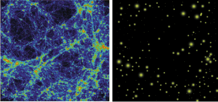
The non-linear evolution of the dark matter distribution has also been studied extensively using numerical simulations of the large scale structure clustering process. These simulations show that an initially smooth matter distribution evolves into a complex network of sheets, filaments and knots (e.g., figure 1). The dense knots are often called dark matter halos. High resolution, but relatively small volume, simulations have been used to provide detailed information about the distribution of mass in and around such halos (i.e., the halo density profile of [198, 195]), whereas larger volume, but lower resolution simulations (e.g., the Hubble Volume simulations [80] of the Virgo consortium[278]), have provided information about the abundance and spatial distribution of halos [135, 41]. Simulations such as these show that the halo abundance, spatial distribution, and internal density profiles are closely related to the properties of the initial fluctuation field. When these halos are treated as the analogs of Neyman & Scott’s clusters, their formalism provides a way to describe the spatial statistics of the dark matter density field from the linear to highly non-linear regimes.

Figure 2: Distribution of galaxies (in color) superposed on the dark matter distribution (grey scale) in simulations run by the GIF collaboration [157]. Galaxy colors blue, yellow, green and red represent successively smaller star formation rates. Different panels show how the spatial distributions of dark matter and galaxies evolve; the relation between the two distributions changes with time, as do the typical star formation rates.

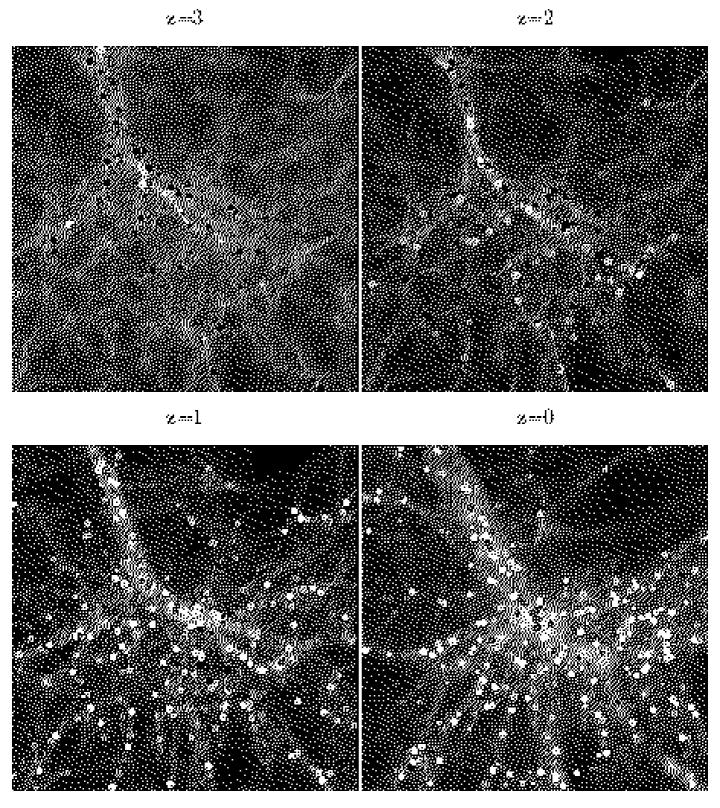
Such a halo based description of the dark matter distribution of large scale structure is extremely useful because, following White & Rees [292], the idea that galaxies form within such dark matter halos has gained increasing credence. In this picture, the physical properties of galaxies are determined by the halos in which they form. Therefore, the statistical properties of a given galaxy population are determined by the properties of the parent halo population. There are now a number of detailed semianalytic models which implement this approach [157, 264, 42, 10]; they combine simple physically motivated galaxy formation recipes with the halo population output from a numerical simulation of the clustering of the dark matter distribution to make predictions about how the galaxy and dark matter distributions differ (see, e.g., Figure 2).

In the White & Rees based models, different galaxy types populate different halos. Therefore, the halo based approach provides a simple and natural way of modelling the dependence of galaxy clustering on galaxy type in these models. It is also the natural way of modelling the difference between the clustering of galaxies relative to dark matter.

Just as the number of galaxies in a randomly placed cell may be a biased tracer of the amount of dark matter in it, other physical properties such as the pressure, the velocity or the momentum, of a cell are also biased tracers of the amount of dark matter a cell contains. The assumption that dark matter halos are in virial equilibrium allows one to estimate these physical properties for any given halo. If the distribution of halos in a randomly chosen cell is known, then the halo–based approach allows one to estimate statistical properties of, say, the pressure and the momentum, analogously to how it transforms the statistics of the dark matter field into that for galaxies.

Data from large area imaging and redshift surveys of galaxies (e.g., the 2dFGRS and the Sloan Digital Sky Survey) are now becoming available; these will provide constraints on the dark matter distribution on large scales, and on galaxy formation models on smaller scales. Weak gravitational lensing [146] provides a more direct probe of the dark matter density field. The first generation of wide-field weak lensing surveys, which cover a few square degrees are now complete (see recent reviews by Bartlemann & Schneider [7] and Mellier [186]), and the next generation of lensing surveys will cover several hundreds of square degrees. The Sunyaev-Zel’dovich (SZ) effect [274], due to the inverse-Compton scattering of cosmic microwave background (CMB) photons off hot electrons in clusters, is a probe of the distribution of the pressure on large scales. Several wide-field surveys of the SZ are currently planned (see review by Birkinshaw [17]). In addition, the next generation CMB experiments will measure temperature fluctuations on small angular scales. On these small scales the density, velocity, momentum and pressure fields of the dark and/or baryonic matter leave their imprints on the CMB in a wide variety of ways. For example, in addition to the thermal and kinematic SZ effects, the small scale temperature fluctuations are expected to be weakly lensed. The halo model provides a single self-consistent framework for modelling and interpretting all these observations.

The purpose of this review is twofold. The first is to outline the principles which underly the halo approach. The second is to compare the predictions of this approach with results from simulations and observations. Section 1 introduces background materials which are relevant for this review. Sections 2 to 5 present the halo approach to clustering. What we know about dark matter halos is summarized in §3, how this information is incorporated into the halo model is discussed in §4, and the first result, the halo model description of the dark matter density field is presented in §5. The galaxy distribution is discussed in §6, the velocity and momentum fields are studied in §7, weak gravitational lensing in §8, and secondary effects on the cosmic microwave background, including the thermal and kinetic Sunyaev-Zel’dovich effects [274, 206], and the non-linear integrated Sachs-Wolfe effect [229, 222], are the subject of §9.

We have chosen to discuss those aspects of the halo model which are relevant for the statistical studies of clustering, such as the two-point correlation functions and higher order statistics. We do not discuss what cosmological and astrophysical information can be deduced from the redshift distribution and evolution of halo number counts. The abundance of halos at high redshift is an important ingredient in models of reionization and the early universe. We do not discuss any of these models here, since they are described in the recent review by Barkana & Loeb [8]. Finally, our description of the clustering of halos relies on some results from perturbation theory which we do not derive in detail here. For these, we refer the reader to the recent comprehensive review on the pertubation theory description of gravitational clustering by Bernardeau et al. [15].

2 Background Materials

This section describes the properties of adiabatic cold dark matter (CDM) models which are relevant to the present review.

The expansion rate for adiabatic CDM cosmological models with a cosmological constant is

$$H^{2}(z)=H_{0}^{2}\left[\Omega_{m}(1+z)^{3}+\Omega_{K}(1+z)^{2}+\Omega_{\Lambda}\right]\,,$$ (1)

where $H_{0}$ can be written as the inverse Hubble distance today $cH_{0}^{-1}=2997.9h^{-1}$Mpc. The critical density is $\rho_{crit}=3H^{2}/8\pi G$. The total density is a sum over different components $i$, where $i=c$ for the cold dark matter, $\Lambda$ for the cosmological constant, and $b$ for baryons. Our convention will be to denote the contribution to the total density from component $i$, as $\Omega_{i}=\rho_{i}/\rho_{crit}$. The contribution of spatial curvature to the expansion rate is $\Omega_{K}=1-\sum_{i}\Omega_{i}$, and the matter density is $\Omega_{m}=\Omega_{c}+\Omega_{b}$.

Convenient measures of distance and time include the conformal distance (or lookback time) from the observer at redshift $z=0$

$$r(z)=\int_{0}^{z}{dz^{\prime}\over H(z^{\prime})}\,,$$ (2)

(we have set $c=1$) and the angular diameter distance

$$d_{A}=H_{0}^{-1}\Omega_{K}^{-1/2}\sinh(H_{0}\Omega_{K}^{1/2}r)\,.$$ (3)

Note that as $\Omega_{K}\rightarrow 0$, $d_{A}\rightarrow r$ and we define $r(z=\infty)=r_{0}$.

2.1 Statistical description of random fields

The dark matter density field in the adiabatic CDM model possesses $n-$point correlation functions, defined in the usual way. That is, in real coordinate space, the $n-$point correlation function $\xi_{n}$ of density fluctuations $\delta({\bf x})$ is defined by

$$\langle\delta({\bf x}_{1})\cdots\delta({\bf x}_{n})\rangle_{c}\equiv\xi_{n}({\bf x}_{1},\cdots,{\bf x}_{n}).$$ (4)

Here, we have expressed the density perturbations in the universe as fluctuations relative to the background mean density, $\bar{\rho}$:

$$\delta({\bf r})=\frac{\rho({\bf r})}{\bar{\rho}}-1\,.$$ (5)

If all the ${\bf x}_{i}$ are the same, then

$$\langle\delta\rangle_{c} = \langle\delta\rangle$$ (6)

$$\langle\delta^{2}\rangle_{c} = \langle\delta^{2}\rangle-\langle\delta\rangle_{c}^{2}\equiv\sigma^{2}$$ (7)

$$\langle\delta^{3}\rangle_{c} = \langle\delta^{3}\rangle-3\,\langle\delta^{2}\rangle_{c}\,\langle\delta\rangle_{c}-\langle\delta\rangle_{c}^{3}$$ (8)

$$\langle\delta^{4}\rangle_{c} = \langle\delta^{4}\rangle-4\,\langle\delta^{3}\rangle_{c}\,\langle\delta\rangle_{c}-3\,\langle\delta^{2}\rangle_{c}^{2}-6\langle\delta^{2}\rangle_{c}\,\langle\delta\rangle_{c}^{2}-\langle\delta\rangle_{c}^{4}.$$ (9)

We will almost always consider the case in which $\langle\delta\rangle=0$.

Many of the calculations to follow simplify considerably in Fourier space. Throughout, we will use the following Fourier space conventions:

$$A({{\mathbf{x}}}) = \int\frac{d^{3}{\bf k}}{(2\pi)^{3}}\,A({{\bf k}})\,\exp({\rm i}{\bf k}\cdot{\bf x})\qquad{\rm and}$$

$$\delta_{\rm D}({\bf k}_{1\ldots i}) = \int\frac{d^{3}{\bf x}}{(2\pi)^{3}}\,\exp[-{\rm i}{\bf x}\cdot({\bf k}_{1}+\cdots+{\bf k}_{i})]\,$$ (10)

for the Dirac delta function, which is not to be confused with the density perturbation which does not have the subscript $D$.

Thus, the real space fluctuations in the density field is a sum over Fourier modes:

$$\delta({\bf x})=\int{d^{3}{\bf k}\over(2\pi)^{3}}\,\delta({\bf k})\,\exp({\rm i}{\bf k}\cdot{\bf x})$$ (11)

and the two, three and four-point Fourier-space correlations are

$$\langle\delta({\bf k}_{1})\,\delta({\bf k}_{2})\rangle = (2\pi)^{3}\,\delta_{\rm D}({\bf k}_{12})\,P(k_{1})\,,$$ (12)

$$\langle\delta({\bf k}_{1})\,\delta({\bf k}_{2})\,\delta({\bf k}_{3})\rangle = (2\pi)^{3}\,\delta_{\rm D}({\bf k}_{123})\,B({\bf k}_{1},{\bf k}_{2},{\bf k}_{3})\,,$$ (13)

$$\langle\delta({\bf k}_{1})\ldots\delta({\bf k}_{4})\rangle_{c} = (2\pi)^{3}\,\delta_{\rm D}({\bf k}_{1234})\,T({\bf k}_{1},{\bf k}_{2},{\bf k}_{3},{\bf k}_{4})\,,$$ (14)

where ${\bf k}_{i\ldots j}={\bf k}_{i}+\ldots+{\bf k}_{j}$. The quantities $P$, $B$ and $T$ are known as the power spectrum, bispectrum and trispectrum, respectively. Notice that

$$\xi_{2}(r)=\int\frac{d^{3}{\bf k}}{(2\pi)^{3}}\,P(k)\,\exp({\rm i}{\bf k}\cdot{\bf r});$$ (15)

the two-point correlation function and the power spectrum are Fourier transform pairs. Similarly, we can relate higher order correlations and their Fourier space analogies.

Rather than working with $P(k)$ itself, it is often more convenient to use the dimensionless quantity

$$\Delta(k)\equiv{k^{3}\,P(k)\over 2\pi^{2}}\,,$$ (16)

which is the power per logarithmic interval in wavenumber. Similarly, we can define a scaled dimensionless quantity for the Nth Fourier space correlation such that it scales roughly as the logarithmic power spectrum defined above:

$$\Delta_{N}({\bf k}_{1},...,{\bf k}_{N})=\frac{k^{3}}{2\pi^{2}}\left[P_{N}({\bf k}_{1},...,{\bf k}_{N})\right]^{\frac{1}{N}}\,.$$ (17)

We will also often use the quantity

$$\sigma^{2}(R)=\int{dk\over k}\,{k^{3}\,P(k)\over 2\pi^{2}}\,|W(kR)|^{2};$$ (18)

this is the variance in the smoothed density field when the smoothing window has scale $R$. If the window is a tophat in real space, then $W(kR)=[3/(kR)^{3}](\sin kR-(kR)\cos kR)$; it is $\exp(-k^{2}R^{2}/2)$ if the real space smoothing window is a Gaussian: $\exp[-(r/R)^{2}/2]/\sqrt{2\pi R^{2}}$.

The initial perturbations due to inflation are expected to be Gaussian [268, 109, 98, 5, 160], so they can be characterized by a power spectrum or a two point correlation function (Wick’s theorem states that, for a Gaussian field, correlations involving an odd number of density fluctuations are exactly zero). Thus, the bispectrum and trispectrum are defined so that, for a Gaussian field, they are identically zero; in the jargon, this means that only the connected piece is used to define them, hence the subscript $c$ in the expression equation (14). All these quantities evolve. Here and throughout, we do not explicitly write the redshift dependence when we believe no confusion will arise.

2.2 Results from perturbation theory

The large scale structure we see today is thought to be due to the gravitational evolution of initially Gaussian fluctuations [217, 18, 64]. In an expanding universe filled with CDM particles, the action of gravity results in the generation of higher order correlations: the initially Gaussian distribution becomes non-Gaussian. The perturbation theory description of the gravitational evolution of density perturbations is well developed [15]. Here we briefly summarize some of the results which are most relevant for what is to follow.

The evolution of large scale structure density perturbations are governed by the continuity equation,

$$\frac{\partial\delta}{\partial t}+\frac{1}{a}\nabla\cdot(1+\delta){\bf u}=0\,,$$ (19)

and the Euler equation,

$$\frac{\partial\delta}{\partial t}+H{\bf u}+\frac{1}{a}\left[({\bf u}\cdot\nabla){\bf u}+\nabla\phi\right]=0\,,$$ (20)

where the potential fluctuations due to density perturbations are related by the Poisson equation:

$$\nabla^{2}\phi=4\pi G\bar{\rho}a^{2}\delta,$$ (21)

while the peculiar velocity is related to the Hubble flow via

$${\bf u}={\bf v}-H{\bf x}\,.$$ (22)

The linear regime is the one in which $\delta\ll 1$. In the linear regime, the continuity and Euler equations may be combined to yield [216]

$$\frac{\partial^{2}\delta}{\partial t^{2}}+2H\frac{\partial\delta}{\partial t}-4\pi G\bar{\rho}\delta=0\,.$$ (23)

This is a second-order differential equation with two independent solutions; these correspond to modes which grow and decay with time. For our purposes, only the growing mode solution of equation (23) is relevant. This has the form [216]

$$\delta(k,r)=G(r)\,\delta(k,0),$$ (24)

where

$$G(r) \propto {H(r)\over H_{0}}\int_{z(r)}^{\infty}dz^{\prime}(1+z^{\prime})\left[{H_{0}\over H(z^{\prime})}\right]^{3}$$ (25)

$$\approx {5\over 2}{\Omega_{m}(z)/(1+z)\over\Omega_{m}(z)^{4/7}-\Omega_{\Lambda}(z)+(1-\Omega_{m}(z)/2)(1+\Omega_{\Lambda}(z)/70)}.$$

This shows that the linear theory density field may be scaled in time, or redshift, with the use of the growth solution $G(z)$. Note that $G\propto a=(1+z)^{-1}$ as $\Omega_{m}\to 1$. The approximation in the second line of equation (25) is good to a few percent [164, 167, 34].

In linear perturbation theory, the power spectrum of the initial density fluctuation field is

$$\frac{k^{3}P^{\rm lin}(k)}{2\pi^{2}}=\delta_{H}^{2}\,\left({k\over H_{0}}\right)^{n+3}T^{2}(k)\,.$$ (26)

Here, $n$ is said to be the slope of the initial spectrum. A scale free form for $P(k)\sim k^{n}$ is rather generic; models of inflation generally produce $n\sim 1$ (the so-called Harrison-Zel’dovich spectrum [108, 299, 214]). The quantity $T(k)$, defined such that $T(0)=1$, describes departures from the initially scale free form. Departures are expected because the energy density of the Universe is dominated by radiation at early times but by matter at late times, and the growth rate of perturbations in the radiation dominated era differs from that in the matter dominated era. The transition from one to the other produces a turnover in the shape of the power spectrum [20, 18]. Baryons and other species, such as massive neutrinos, leave other important features in the transfer function which can potentially be extracted from observational data. Accurate fitting functions for $T(k)$ which include these effects have been available for some time [6, 117, 73]. When illustrating calculations presented in this review, we use fits to the transfer functions given by [74].

When written in comoving coordinates, the continuity equation (19) shows that the Fourier transforms of the linear theory (i.e., when $\delta\ll 1$) density and velocity fields are related [216]:

$${\bf u}({\bf k})=-i\,\dot{G}\,\delta(k)\,\frac{{\bf k}}{k^{2}}\,,$$ (27)

where the derivative is with respect to the radial distance $r(z)$ defined in equation (2). This shows that the power spectrum of linear theory velocities is

$$P^{\rm lin}_{\rm vel}(k)=\frac{\dot{G}^{2}}{k^{2}}P^{\rm lin}(k)\,.$$ (28)

The fluctuations in the linear density field are also simply related to to those in the potential [4]. In particular, the Fourier transform of the Poisson equation (21) shows that

$$\Phi(k)=\frac{3}{2}\Omega_{m}\left(\frac{H_{0}}{k}\right)^{2}\left[1+3\left(\frac{H_{0}}{k}\right)^{2}\Omega_{K}\right]^{-2}\left(\frac{G}{a}\right)\,\delta(k)\,.$$ (29)

Since gravity induces higher order correlations in the density field, perturbation theory can be used to calculate them also. The bispectrum, i.e., the Fourier transform of the three point correlation function of density perturbations, can be calculated using second order perturbation theory [93, 178, 132]:

$$B^{\rm lin}({\bf k}_{p},{\bf k}_{q},{\bf k}_{r}) = 2F_{2}^{\rm s}({\bf k}_{p},{\bf k}_{q})P(k_{p})P(k_{q})+2\;{\rm Perm.},$$

where

$$F_{2}^{\rm s}({\bf q}_{1},{\bf q}_{2})=\frac{1}{2}\left[(1+\mu)+\frac{{\bf q}_{1}\cdot{\bf q}_{2}}{q_{1}q_{2}}\left(\frac{q_{1}}{q_{2}}+\frac{q_{2}}{q_{1}}\right)+(1-\mu)\frac{({\bf q}_{1}\cdot{\bf q}_{2})^{2}}{q_{1}^{2}q_{2}^{2}}\right]\,.$$ (31)

The bispectrum depends only weakly on $\Omega_{m}$, the only dependence coming from the fact that $\mu\approx(3/7)\Omega_{m}^{-2/63}$ for $0.05<\Omega_{m}<3$ [153].

The expressions above show that, in perturbation theory, the bispectrum generally scales as the square of the power spectrum. Therefore, it is conventional to define a reduced bispectrum:

$$Q_{123}\equiv\frac{B_{123}}{P_{1}P_{2}+P_{2}P_{3}+P_{3}P_{1}}.$$ (32)

To lowest order in perturbation theory, $Q$ is independent of time and scale [85, 86]. When the $k$ vectors make an equililateral triangle configuration, then

$$Q_{\rm eq}(k)\equiv{1\over 3}\left[{\Delta_{\rm eq}^{2}(k)\over\Delta^{2}(k)}\right]^{2},\quad{\rm where}\quad\Delta_{\rm eq}^{2}(k)\equiv\frac{k^{3}}{2\pi^{2}}\sqrt{B(k,k,k)}$$ (33)

represents the bispectrum for equilateral triangle configurations. In second order perturbation theory,

$$Q_{\rm eq}^{\rm PT}=1-\frac{3}{7}\Omega_{m}^{-2/63};$$ (34)

this should be a good approximation on large scales.

Similarly, the perturbation theory trispectrum is

$$T^{\rm lin}=4\left[F_{2}^{\rm s}({\bf k}_{12},-{\bf k}_{1})F_{2}^{\rm s}({\bf k}_{12},{\bf k}_{3})\,P(k_{1})P(k_{12})P(k_{3})+{\rm Perm.}\right]$$

$$\qquad\qquad+6\left[F_{3}^{\rm s}({\bf k}_{1},{\bf k}_{2},{\bf k}_{3})P(k_{1})P(k_{2})P(k_{3})+{\rm Perm.}\right]\,;$$ (35)

there are 12 permutations in the first set and 4 in the second [86]. The function $F_{3}^{\rm s}$ can be derived through a recursion relation [93, 132, 178]

$$F_{n}^{\rm s}({\bf q}_{1},...,{\bf q}_{n}) = \sum_{m=1}^{n-1}\frac{G_{m}^{\rm s}({\bf q}_{1},...,{\bf q}_{m})}{(n-1)(2n+3)}\Big{[}(2n+1)\frac{{\bf q}_{1,n}\cdot{\bf q}_{1,m}}{{\bf q}_{1,m}\cdot{\bf q}_{1,m}}F_{n-m}^{\rm s}({\bf q}_{m+1},...,{\bf q}_{n})$$ (36)

$$\ +\ \frac{({\bf q}_{1,n}\cdot{\bf q}_{1,n})({\bf q}_{1,m}\cdot{\bf q}_{m+1,n})}{({\bf q}_{1,m}\cdot{\bf q}_{1,m})({\bf q}_{m+1,n}\cdot{\bf q}_{m+1,n})}G_{n-m}^{\rm s}({\bf q}_{m+1},...,{\bf q}_{n})\Big{]}$$

with ${\bf q}_{a,b}={\bf q}_{a}+...+{\bf q}_{b}$, $F_{1}^{\rm s}=G_{1}^{\rm s}=1$ and

$$G_{2}^{\rm s}({\bf q}_{1},{\bf q}_{2})=\mu+\frac{1}{2}\frac{{\bf q}_{1}\cdot{\bf q}_{2}}{q_{1}q_{2}}\left(\frac{q_{1}}{q_{2}}+\frac{q_{2}}{q_{1}}\right)+(1-\mu)\frac{({\bf q}_{1}\cdot{\bf q}_{2})^{2}}{q_{1}^{2}q_{2}^{2}}\,,$$ (37)

where $\mu$ has the dependence on $\Omega_{m}$ as in $F_{2}^{\rm s}$ (equation 31). The factor of 2 in equation (LABEL:eqn:bpt) and the factors of 4 and 6 in equation (35) are due to the use of symmetric forms of the $F_{n}^{\rm s}$. Once again, it is useful to define

$$Q_{1234}\equiv\frac{T_{1234}}{[P_{1}P_{2}P_{13}+{\rm cyc.}]+[P_{1}P_{2}P_{3}+{\rm cyc.}]},$$ (38)

where the permutations include 8 and 4 terms respectively in the ordering of $(k_{1},k_{2},k_{3},k_{4})$. For a square configuration,

$$Q_{\rm sq}(k)\equiv\frac{T({\bf k},-{\bf k},{\bf k}_{\perp},-{\bf k}_{\perp})}{[8P^{2}(k)P(\sqrt{2}k)][4P^{3}(k)]}\,.$$ (39)

In perturbation theory, $Q_{\rm sq}\approx 0.085$.

The perturbation theory description of clustering also makes predictions for correlations in real space. For clustering from Gaussian initial conditions, the higher order moments of the dark matter distribution in real space satisfy

$$\langle\delta^{n}\rangle=S_{n}\,\langle\delta^{2}\rangle^{n-1},\qquad{\rm if}\qquad\langle\delta^{2}\rangle\ll 1,$$ (40)

where the $S_{n}$ are numerical coefficients which are approximately independent of scale over a range of large scales on which $\langle\delta^{2}\rangle\ll 1$. These coefficients are [12]

$$S_{3}^{\rm lin} = \frac{34}{7}+\gamma_{1},\qquad S_{4}^{\rm lin}=\frac{60712}{1323}+\frac{62}{3}\gamma_{1}+\frac{7}{3}\gamma_{1}^{2}+\frac{2}{3}\gamma_{2},\quad{\rm and}$$

$$S_{5}^{\rm lin} = \frac{200575880}{305613}+\frac{1847200}{3969}\gamma_{1}+\frac{1490}{63}\gamma_{2}+\frac{50}{9}\gamma_{1}\gamma_{2}+\frac{10}{27}\gamma_{3}\,,$$ (41)

where

$$\gamma_{j}\equiv\frac{d^{j}\ln\sigma^{2}(R)}{d(\ln R)^{j}}\,$$ (42)

and $\sigma(R)$ is defined by inserting the linear theory value of $P^{\rm lin}(k)$ in equation (18). Note that $\gamma_{1}=-(n+3)$ and $\gamma_{i}=0$ for $i>1$ if the initial spectrum is a power-law with slope $n$. For the CDM family of spectra, one can neglect derivatives of $\sigma^{2}(R)$ with respect to scale for $R\leq 20$ $h^{-1}$ Mpc. Also note that the $S_{n}^{\rm lin}$ depend only slightly on cosmology: e.g., the skewness is $S_{3}^{\rm lin}=4+\frac{6}{7}\Omega_{m}^{-2/63}+\gamma_{1}$ [29, 114, 84].

Although all derivations to follow will be general, we will often illustrate our results with the currently favored $\Lambda$CDM cosmological model. Following the definition of the expansion rate (equation 1) and the power spectrum of linear density field (equation 26), the relevant parameters for this model are $\Omega_{c}=0.30$, $\Omega_{b}=0.05$, $\Omega_{\Lambda}=0.65$, $h=0.65$, and $n=1$.

The associated power spectrum of linear fluctuations is normalized to match the observed anisotropy in the cosmic microwave background at the largest scales, i.e., those measured by the COBE mission. This means [32] that we set $\delta_{H}=4.2\times 10^{-5}$. A constraint on the shape of the spectrum also follows from specifying the amplitude of the power spectrum on a smaller scale. This additional constraint is usually phrased as requiring that $\sigma_{8}$, the rms value of the linear density fluctuation field when it is smoothed with a tophat filter of scale $R=8h^{-1}$ Mpc (i.e., $\sigma_{8}$ is calculated using equation 18 with $R=8h^{-1}$ Mpc), has a specified value. This value is set by requiring that the resulting fluctuations are able to produce the observed abundance of galaxy clusters. Uncertainties in the conversion of X-ray flux, or temperature, to cluster mass, yield values for $\sigma_{8}$ which are in the range (0.5 – 0.6)$\Omega_{m}^{-(0.5-0.6)}$ [77, 284]. Another constraint on the value of $\sigma_{8}$ is that when properly evolved to past, the same density power spectrum should also match associated fluctuations in the CMB; the two constraints are generally in better agreement in a cosmology with a cosmological constant than in an open universe. The use of a realistic value for $\sigma_{8}$ is important because higher order correlations typically depend non-linearly on the amplitude of the initial linear density field.

2.3 Beyond perturbation theory

The following ansatz, due to [102], provides a good description of the two-point correlations in real space, $\xi_{2}(r)$, and in Fourier space, $P(k)$, even in the regime where perturbation theory becomes inaccurate. The argument is that non-linear gravitational evolution rescales all lengths, so pairs initially separated by scale $r_{\rm L}$ will later be separated by a different scale, say $r_{\rm NL}$. The initial and final scales are related by

$$r_{\rm NL}={r_{\rm L}\over[1+\bar{\xi}_{\rm NL}(r_{\rm NL})]^{1/3}}\qquad{\rm where}\qquad\bar{\xi}_{\rm NL}(x)={3\over x^{3}}\int_{0}^{x}dr\ r^{2}\,\xi_{2}(r).$$ (43)

The ansatz is that there exists some universal function

$$\bar{\xi}_{\rm NL}(r_{\rm NL})=X_{\rm NL}\Bigl{[}\bar{\xi}_{\rm L}(r_{\rm L})\Bigr{]}.$$ (44)

This is motivated by noting that $\bar{\xi}_{\rm NL}(r_{\rm NL})\propto\bar{\xi}_{\rm L}(r_{\rm L})$ in the linear regime where $\bar{\xi}_{\rm NL}\ll 1$, and $\bar{\xi}_{\rm NL}(r_{\rm NL})\propto[\bar{\xi}_{\rm L}(r_{\rm L})]^{3/2}$ in the highly non-linear regime where $\bar{\xi}\gg 1$. The 3/2 scaling comes if $\bar{\xi}_{\rm NL}\propto a^{3}$ in the highly non-linear regime (this is expected if, on the smallest scales, the expansion of the background is irrelevant), whereas $\bar{\xi}_{\rm L}\propto a^{2}$. In the intermediate regime, it has been argued that $\bar{\xi}_{\rm NL}(r_{\rm NL})\propto[\bar{\xi}_{\rm L}(r_{\rm L})]^{3}$ [202]. The exact transitions between the different regimes, however, must be calibrated using numerical simulations.

For similar reasons, one expects a scaling for the non-linear power spectrum

$$k_{\rm L}={k_{\rm NL}\over[1+\Delta_{\rm NL}(k_{\rm NL})]^{1/3}}\qquad{\rm with}\qquad\Delta_{\rm NL}(k_{\rm NL})=f_{\rm NL}\Bigl{[}\Delta_{\rm L}(k_{\rm L})\Bigr{]}.$$ (45)

Fitting formulae for $X_{\rm NL}$ and $f_{\rm NL}$, obtained by calibrating to numerical simulations, are given in [209, 131]; in what follows we will use the fits given by [210] for the power spectrum with

$$f_{\rm NL}(x)=x\left[\frac{1+B\beta x+\left(Ax\right)^{\alpha\beta}}{1+\left(\left[Ax\right]^{\alpha}g^{3}/\left[Vx^{1/2}\right]\right)^{\beta}}\right]^{1/\beta}\,,$$ (46)

where,

$$A = 0.482\left(1+\frac{n}{3}\right)^{-0.947}\;\;\;B=0.226\left(1+\frac{n}{3}\right)^{-1.778}$$

$$\alpha = 3.310\left(1+\frac{n}{3}\right)^{-0.244}\;\;\;\beta=0.862\left(1+\frac{n}{3}\right)^{-0.287}$$

$$V = 11.55\left(1+\frac{n}{3}\right)^{-0.423}\,,$$ (47)

and

$$n(k_{L})=\frac{d\,{\rm ln}\,P}{d\,{\rm ln}\,k}\Big{|}_{k=k_{L}/2}\,.$$ (48)

Note that in equation (46), the redshift dependence comes only from the factor of $g^{3}$, where $g$ is the growth suppression factor relative to an $\Omega_{m}=1$ universe: $g=(1+z)\,G(z)$, with $G(z)$ the linear growth factor given in equation (25). The parameters of the above fit come from a handful of simulations and are valid for a limited number of cosmological models. Fits to the non-linear power spectrum in some cosmological models containing dark energy are provided by [171].

Although this ansatz, and the associated fitting function represents a significant step beyond perturbation theory, there have been no successful extensions of it to higher order clustering statistics. In addition, it is not obvious how to extend it to describe fields other than the density of dark matter.

Hyper-extended perturbation theory (HEPT; [238]) represents a reasonably successful attempt to extract what is known from perturbation theory and apply it in the highly nonlinear regime. This model makes specific predictions about higher order clustering. For example,

$$Q_{\rm eq}^{\rm HEPT}(k)=\frac{4-2^{n}}{1+2^{n+1}}\quad{\rm and}\quad Q_{\rm sq}^{\rm sat}=\frac{1}{2}\left[\frac{54-27\cdot 2^{n}+2\cdot 3^{n}+6^{n}}{1+6\cdot 2^{n}+3\cdot 3^{n}+6\cdot 6^{n}}\right],$$ (49)

where $n(k)$ is the linear power spectral index at $k$. Fitting functions for $Q_{\rm eq}(k)$ for $0.1\mathchar 13358\relax k\mathchar 13358\relax 3h$ Mpc^-1, calibrated from numerical simulations, can be found in [239].

3 Dark Matter Halo Properties

In this section, and the next, we will describe an approach which allows one to describe all $n-$point correlations of large scale structure. This description can be used to study clustering of a variety of physical quantities, including the dark matter density field, the galaxy distribution, the pressure, the momentum, and others.

The approach assumes that all the mass in the Universe is partitioned up into distinct units, which we will often call halos. If distinct halos can be identified, then it is likely that they are small compared to the typical distances between them. This then suggests that the statistics of the mass density field on small scales are determined by the spatial distribution within the halos; the precise way in which the halos themselves may be organized into large scale structures is not important. On the other hand, the details of the internal structure of the halos cannot be important on scales larger than a typical halo; on large scales, the important ingredient is the spatial distribution of the halos. This realization, that the distribution of the mass can be studied in two steps: the distribution of mass within each halo, and the spatial distribution of the halos themselves, is the key to what has come to be called the halo model.

The halo model assumes that, in addition to thinking of the spatial statistics in two steps, it is useful and accurate to think of the physics in two steps also. In particular, the model assumes that the regime in which the physics is not described by perturbation theory is confined to regions within halos, and that halos can be adequately approximated by assuming that they are in virial equilibrium.

Clearly, then, the first and the most important step is to find a suitable definition of the underlying units, i.e. the halos. This section describes what we know about the abundance, spatial distribution, and internal density profiles of halos. All these quantities depend primarily on halo mass. In the next section, we combine these ingredients together to build the halo model of large scale structure.

3.1 The spherical collapse model

The assumption that non-linear objects formed from a spherical collapse is a simple and useful approximation. The spherical collapse of an initially tophat density perturbation was first studied in 1972 by Gunn & Gott [96]; see [82, 16] for a discussion of spherical collapse from other initial density profiles.

In the tophat model, one starts with a region of initial, comoving Lagrangian size $R_{0}$. Let $\delta_{i}$ denote the initial density within this region. We will suppose that the initial fluctuations were Gaussian with an rms value on scale $R_{0}$ which was much less than unity. Therefore, $|\delta_{i}|\ll 1$ almost surely. This means that the mass $M_{0}$ within $R_{0}$ is $M_{0}=(4\pi R_{0}^{3}/3)\bar{\rho}(1+\delta_{i})\approx(4\pi R_{0}^{3}/3)\bar{\rho}$ where $\bar{\rho}$ denotes the comoving background density.

As the Universe evolves, the size of this region changes. Let $R$ denote the comoving size of the region at some later time. The density within the region is $(R_{0}/R)^{3}\equiv(1+\delta)$. In the spherical collapse model there is a deterministic relation between the initial comoving Lagrangian size $R_{0}$ and density of an object, and its Eulerian size $R$ at any subsequent time. For an Einstein–de Sitter universe, one can obtain a parametric solution to $R(z)$ in terms of $\theta$:

$${R(z)\over R_{0}}={(1+z)\over(5/3)\,|\delta_{0}|}\,{(1-\cos\theta)\over 2}\quad{\rm and}\quad{1\over 1+z}=\left({3\over 4}\right)^{2/3}{(\theta-\sin\theta)^{2/3}\over(5/3)\,|\delta_{0}|},$$ (50)

where $\delta_{0}$ denotes the initial density $\delta_{i}$ extrapolated using linear theory to the present time (e.g. [216]). If $\delta_{i}<0$, then $(1-\cos\theta)$ should be replaced with $(\cosh\theta-1)$ and $(\theta-\sin\theta)$ with $(\sinh\theta-\theta)$.

In the spherical collapse model, initially overdense regions collapse: with $\theta=0$ at start, they ‘turnaround’ at $\theta=\pi$, and have collapsed completely when $\theta=2\pi$. Equation (50) shows that the size of an overdense region evolves as

$${R_{0}\over R(z)}={6^{2/3}\over 2}{(\theta-\sin\theta)^{2/3}\over(1-\cos\theta)}.$$ (51)

At turnaround, $\theta=\pi$, so $[R_{0}/R(z_{\rm ta})]^{3}=(3\pi/4)^{2}$; when an overdense region turns around, the average density within it is about 5.55 times that of the background universe.

At collapse, the average density within the region is even higher: formally, $R(z_{\rm col})=0$, so the density at collapse is infinite. In practice the region does not collapse to vanishingly small size: it virializes at some non-zero size. The average density within the virialized object is usually estimated as follows. Assume that after turning around the object virializes at half the value of the turnaround radius in physical, rather than comoving units. In the time between turnaround and collapse, the background universe expands by a factor of $(1+z_{\rm ta})/(1+z_{\rm col})=2^{2/3}$ (from equation 50), so the virialized object is eight times denser than it was at turnaround (because $R_{\rm vir}=R_{\rm ta}/2$). The background density at turnaround is $(2^{2/3})^{3}=4$ times the background density at $z_{\rm vir}$. Therefore, the virialized object is

$$\Delta_{\rm vir}\equiv(9\pi^{2}/16)\times 8\times 4=18\pi^{2}\,,$$ (52)

times the density of the background at virialization.

What was the initial overdensity of such an object? The first of equations (50) shows that if the region is to collapse at $z$, the average density within it must have had a critical value, $\delta_{\rm sc}$, given by

$${\delta_{\rm sc}(z)\over 1+z}={3\over 5}\,\left({3\pi\over 2}\right)^{2/3}.$$ (53)

Thus, a collapsed object is one in which the initial overdensity, extrapolated using linear theory to the time of collapse, was $\delta_{\rm sc}(z)$. At this time, the actual overdensity is significantly larger than the linear theory prediction. Although the formal overdensity is infinite, a more practical estimate (equation 52) says that the object is about 178 times denser than the background.

There is an important feature of the spherical collapse model which is extremely useful. Since $(1+\delta)=(R/R_{0})^{3}$, the equations above provide a relation between the actual overdensity $\delta$, and that predicted by linear theory, $\delta_{0}$, and this relation is the same for all $R_{0}$. That is to say, it is the ratio $R/R_{o}$ which is determined by $\delta_{i}$, rather than the value of $R$ itself. Because the mass of the object is proportional to $R_{0}^{3}$, this means that the critical density for collapse $\delta_{\rm sc}$ is the same for all objects, whatever their mass. In addition, the evolution of the average density within a region which is collapsing is also independent of the mass within it (of course, it does depend on the initial overdensity).

To see what this relation is, note that the parametric solution of equation (50) can be written as a formal series expansion, the first few terms of which are [13]

$${\delta_{0}\over 1+z}=\sum_{k=0}^{\infty}a_{k}\,\delta^{k}=\delta-{17\over 21}\,\delta^{2}+{341\over 567}\,\delta^{3}-{55805\over 130977}\,\delta^{4}+\ldots$$ (54)

To lowest order this is just the linear theory relation: $\delta$ is the initial $\delta_{0}$ times the growth factor. A good approximation to the spherical collapse relation $\delta_{0}(\delta)$, valid even when $\delta\gg 1$, is [190]

$${\delta_{0}\over 1+z}={3\,(12\pi)^{2/3}\over 20}-{1.35\over(1+\delta)^{2/3}}-{1.12431\over(1+\delta)^{1/2}}+{0.78785\over(1+\delta)^{0.58661}}.$$ (55)

While these are all convenient estimates of the parameters of collapsed objects, it is important to bear in mind that the collapse is seldom spherical, and that the estimate for the virial density is rather adhoc. Descriptions of ellipsoidal collapse have been considered [129, 21, 194, 257], as have alternative descriptions of the $\delta_{0}(\delta)$ relation [79]. In most of what follows, we will ignore these subtleties.

Though we have used an Einstein-de Sitter model to outline several properties related to spherical collapse, our discussion remain qualitatively similar in cosmologies for which $\Omega_{m}\leq 1$ and/or $\Omega_{\Lambda}\geq 0$. The actual values of $\delta_{\rm sc}$ and $\Delta_{\rm vir}$ depend on cosmology: fitting functions for these are available in the literature [77, 198, 197, 24, 112].

3.2 The average number density of halos

Let $n(m,z)$ denote the comoving number density of bound objects, halos, of mass $m$ at redshift $z$. (Some authors use $dn/dm$ to denote this same quantity, and we will use the two notations interchangeably.) Since halos formed from regions in the initial density field which were sufficiently dense that they later collapsed, to estimate $n(m,z)$, we must first estimate the number density of regions in the initial fluctuation field which were dense enough to collapse. A simple model for this was provided by Press & Schechter in Ref. [219]:

$${m^{2}n(m,z)\over\bar{\rho}}\,{{\rm d}m\over m}=\nu f(\nu)\,{{\rm d}\nu\over\nu},$$ (56)

where $\bar{\rho}$ is the comoving density of the background with

$$\nu f(\nu)=\sqrt{\nu\over 2\pi}\ \exp(-\nu/2),\qquad{\rm and}\qquad\nu\equiv{\delta^{2}_{\rm sc}(z)\over\sigma^{2}(m)}.$$ (57)

Here $\delta_{\rm sc}(z)$ is the critical density required for spherical collapse at $z$, extrapolated to the present time using linear theory. In an Einstein-de Sitter cosmology, $\delta_{\rm sc}(z=0)=1.686$ while in other cosmologies, $\delta_{\rm sc}$ depends weakly on $\Omega_{m}$ and $\Omega_{\Lambda}$ [77]. In equation (57), $\sigma^{2}(m)$ is the variance in the initial density fluctuation field when smoothed with a tophat filter of scale $R=(3m/4\pi\bar{\rho})^{1/3}$, extrapolated to the present time using linear theory:

$$\sigma^{2}_{\rm lin}(m)\equiv\int\frac{{\rm d}k}{k}\,{k^{3}P^{\rm lin}(k)\over 2\pi^{2}}\,|W(kR)|^{2},$$ (58)

where $W(x)=(3/x^{3})\,[\sin(x)-x\cos(x)]$.

A better fit to the number density of halos in simulations of gravitational clustering in the CDM family of models is given by Sheth & Tormen [254]:

$$\nu f(\nu)=A(p)\left(1+(q\nu)^{-p}\right)\,\left({q\nu\over 2\pi}\right)^{1/2}\,\exp(-q\nu/2),$$ (59)

where $p\approx 0.3$, $A(p)=[1+2^{-p}\Gamma(1/2-p)/\sqrt{\pi}]^{-1}\approx 0.3222$, and $q\approx 0.75$. If $p=1/2$ and $q=1$, then this expression is the same as that in equation (57). At small $\nu\ll 1$, the mass function scales as $\nu f(\nu)\propto\nu^{0.5-p}$. Whereas the small mass behavior depends on the value of $p$, the exponential cutoff at $\nu\gg 1$ does not. The value $\nu=1$ defines a characteristic mass scale, which is usually denoted $m_{*}$: $\sigma(m_{*})\equiv\delta_{\rm sc}(z)$ and is $\sim 2\times 10^{13}$ M${}_{\hbox{$\odot$}}$ at $z=0$; note that halos more massive than $m_{*}$ are rare.

Elegant derivations of equation (57) in [71, 211, 19] show that it can be related to a model in which halos form from spherical collapse. When extended to the ellipsoidal collapse model described by [21], the same arguments give equation (59) [257, 256]. Alternative models for the the shape of $n(m,z)$ are available in the literature [1, 180, 166, 106]; we will not consider them further, however, as equation (59) has been found to provide a good description of the mass function in numerical simulations.

Figure 3: The halo mass function in numerical simulations of the Virgo collaboration. The measured mass distribution is show in color; dashed line shows the Press-Schechter mass function; dotted line is a fitting formula which is similar to the Sheth-Tormen mass function. The figure is from [135].

This is shown in Figure 3, which is taken from numerical simulations run by the Virgo collaboration [135]. The jagged lines show the mass function at various output times in the simulation rescaled from mass $m$ to $\sigma(m)$. The figure shows that, when rescaled in this way,

$$f(\sigma,z)\equiv\frac{m}{\bar{\rho}}\frac{dn(m,z)}{d\ln\sigma^{-1}}\,,$$ (60)

is a universal curve (results from all output times in the simulations trace out approximately the same curve). The dashed line shows that this distribution of halo masses is not so well described by equation (57). The dotted line shows

$$f(\sigma)=0.315\exp\left(-|\ln\sigma^{-1}+0.61|^{3.8}\right)\,;$$ (61)

this fitting formula is accurate to 20% in the range $-1.2\leq\ln\sigma^{-1}\leq 1.05$ [135]. It is very well described by equation (59), which is physically motivated, and so it is equation (59) which we will use in what follows.

3.3 The number density of halos in dense regions

Suppose we divide space up into cells of comoving volume $V$. The different cells may contain different amounts of mass $M$, which means they have different densities: $M/V\equiv\bar{\rho}(1+\delta)$. Let $N(m,z_{1}|M,V,z_{0})$ denote the average number of $m$ halos which collapsed at $z_{1}$, and are in cells of size $V$ which contain mass $M$ at $z_{0}$. The overdensity of halos in such cells is

$$\delta_{\rm h}(m,z_{1}|M,V,z_{0})={N(m,z_{1}|M,V,z_{0})\over n(m,z_{1})V}-1.$$ (62)

Since we already have a model for the denominator, to proceed, we need a good estimate of $N(m,z_{1}|M,V,z_{0})$.

A halo is a region which was sufficiently overdense that it collapsed. So the number of halos within $V$ equals the initial size of $V$ times the number density of regions within it which were sufficiently dense that they collapsed to form halos. If $V$ is overdense today, it’s comoving size is smaller than it was initially; the initial comoving size was $M/\bar{\rho}=V(1+\delta)$. If we write $N(m,z_{1}|M,V,z_{0})=n(m,z_{1}|M,V,z_{0})V(1+\delta)$, then we need an estimate of the number density $n(m,z_{1}|M,V,z_{0})$.

The average number density of halos $n(m,z_{1})$ is a function of the critical density required for collapse at that time: $\delta_{\rm sc}(z_{1})$. In the present context, $n(m,z)$ should be thought of as describing the number density of halos in extremely large cells which are exactly as dense as the background (i.e., cells which have $M\to\infty$ and $\delta=0$). Denser cells may be thought of as regions in which the critical density for collapse is easier to reach, so a good approximation to $n(m,z_{1}|M,V,z_{0})$ is obtained by replacing $\delta_{\rm sc}(z)$ in the expression for $n(m,z)$ with $\delta_{\rm sc}(z_{1})-\delta_{0}(\delta,z_{0})$ [190]. Note that we cannot use $\delta$ itself, because $\delta_{\rm sc}(z_{1})$ has been extrapolated from the initial conditions using linear theory, whereas $\delta$, being the actual value of the density, has been transformed from its value in the initial conditions using non-linear theory. Equations (54) and (55) show the spherical collapse model for this non-linear $\delta_{0}(\delta,z)$ relation. Here, $\delta_{0}(\delta,z_{0})$ denotes the initial density, extrapolated using linear theory, which a region must have had so as to have density $\delta$ at $z_{0}$.

Thus, a reasonable estimate of the density of $m$-halos which virialized at $z_{1}$ and are in cells of size $V$ with mass $M$ at $z_{0}$ is

$${m^{2}n(m,z_{1}|M,V,z_{0})\over\bar{\rho}}{{\rm d}m\over m}=\nu_{10}\,f(\nu_{10})\,{{\rm d}\nu_{10}\over\nu_{10}}\ {\rm where}\ \nu_{10}={[\delta_{\rm sc}(z_{1})-\delta_{0}(\delta,z_{0})]^{2}\over\sigma^{2}(m)-\sigma^{2}(M)},\\$$

and $f(\nu)$ is the same functional form which described the unconditional mass function (equation 57 or 59).

Two limits of this expression are interesting. As $V\to\infty$, $\delta\to\infty$ and $\delta_{0}\to\delta_{\rm sc}(z_{0})$ independent of the value of $M$. A region of small size which contains mass $M$, however, is what we call a halo, with mass $M$. Thus, if we are given a halo of mass $M$ at $z_{0}$, then $N(m,z_{1}|M,V=0,z_{0})$ is the average number of subclumps of mass $m$ it contained at the earlier time when $z_{1}\geq z_{0}$. This limit of equation (3.3) gives what is often called the conditional or progenitor mass function [23, 19, 163, 255]. The opposite limit is also very interesting. As $V\to\infty$, $M\to\infty$ as well: in this limit, $\sigma^{2}(M)\to 0$ and $|\delta|\to 0$, and so equation (3.3) reduces to $n(m,z_{1})$, as expected.

Suppose that we are in the large cell limit. By large, we mean that the rms density fluctuation in these cells is much smaller than unity. Thus, $|\delta|\ll 1$ in most cells and we can use equation (54) for $\delta_{0}(\delta)$. Large cells contain large masses, so $M$ in these cells is much larger than the mass $m_{*}$ of a typical halo. In this limit, $\sigma(M)\ll\sigma(m)$ for most values of $m$ allowing one to set $\sigma(M)\to 0$. This leads to

$$n(m,z_{1}|M,V,z_{0})\approx n(m,z_{1})-\delta_{0}(\delta,z_{0})\left({\partial n(m,z_{1})\over\partial\delta_{\rm sc}}\right)_{\delta_{\rm sc}(z_{1})}+\ldots\,,$$ (63)

such that

$$\delta_{\rm h}(m,z_{1}|M,V,z_{0})\approx\delta-(1+\delta)\,\delta_{0}(\delta,z_{0})\ \left({\partial\ {\rm ln}\,n(m,z_{1})\over\partial\delta_{\rm sc}}\right)_{\rm\delta_{\rm sc}(z_{1})}.$$ (64)

Inserting equation (59) for $n(m,z)$ and keeping terms to lowest order in $\delta$ give (e.g., [45, 190, 252, 254])

$$\delta_{\rm h}(m,z_{1}|M,V,z_{0})\approx\delta\,\left(1+{q\nu-1\over\delta_{\rm sc}(z_{1})}+{2p/\delta_{\rm sc}(z_{1})\over 1+(q\nu)^{p}}\right)=b_{1}(m,z_{1})\,\delta,$$ (65)

where $\nu\equiv\delta_{\rm sc}^{2}(z_{1})/\sigma^{2}(m)$. This expression states that the overdensity of halos in very large cells to be linearly proportional to the overdensity of the mass; the constant of proportionality, $b_{1}(m,z_{1})$, depends on the masses of the halos, and the redshifts they virialized, but is independent of the size of the cells.

If $q=1$ and $p=0$, then massive halos (those which have $\nu>1$ or masses greater than the characteristic mass scale of $m_{*}$) have $b_{1}(m,z_{1})>1$ and are said to be biased relative to the dark matter, while less massive halos ($\nu<1$) are anti-biased. Notice that $b_{1}$ can be very large for the most massive halos, but it is never smaller than $1-1/\delta_{\rm sc}(z_{1})$. Equation (53) shows that halos which virialized at the present time (i.e., $z_{1}=0$), have bias factors which are never less than $\approx 0.41$. Since $\delta_{\rm sc}(z_{1})\gg 1$, in equation (53), halos that virialized at early times have bias factors close to unity (See [204, 87, 276] for a derivation of this limiting case which uses the continuity equation.)

Since $M/V\equiv\bar{\rho}(1+\delta)$, the results above show that, in large cells, $n(m|\delta)\approx[1+b_{1}(m)\delta]\,n(m)$. Since $b_{1}(m)\gg 1$ for the most massive halos, they occupy the densest cells. It is well known that the densest regions of a Gaussian random field are more strongly clustered than cells of average density [227, 143, 6]. Therefore, the most massive halos must also be more strongly clustered than low mass halos. This is an important point to which we will return shortly.

3.4 The distribution of halos on large scales: Deterministic biasing

The linear bias formula is only accurate on large scales. If we write

$$\delta_{\rm h}(m,z_{1}|M,V,z_{0})=\sum_{k>0}b_{k}(m,z_{1})\,\delta^{k}$$ (66)

then inserting equation (3.3) in equation (62), setting $\sigma(M)\to 0$, and expanding gives [236, 189]

$$b_{1}(m,z_{1}) = 1+\epsilon_{1}+E_{1},$$

$$b_{2}(m,z_{1}) = 2(1+a_{2})(\epsilon_{1}+E_{1})+\epsilon_{2}+E_{2},$$

$$b_{3}(m,z_{1}) = 6(a_{2}+a_{3})(\epsilon_{1}+E_{1})+3(1+2a_{2})(\epsilon_{2}+E_{2})+\epsilon_{3}+E_{3},$$

$$b_{4}(m,z_{1}) = 24(a_{3}+a_{4})(\epsilon_{1}+E_{1})+12[a_{2}^{2}+2(a_{2}+a_{3})](\epsilon_{2}+E_{2})$$ (67)

$$\qquad\qquad\qquad\qquad\qquad+4(1+3a_{2})(\epsilon_{3}+E_{3})+\epsilon_{4}+E_{4}$$

for the first few coefficients. Here

$$\epsilon_{1} = {q\nu-1\over\delta_{\rm sc}(z_{1})},\qquad\epsilon_{2}={q\nu\over\delta_{\rm sc}(z_{1})}\,\left({q\nu-3\over\delta_{\rm sc}(z_{1})}\right),\qquad\epsilon_{3}={q\nu\over\delta_{\rm sc}(z_{1})}\,\left({q\nu-3\over\delta_{\rm sc}(z_{1})}\right)^{2},$$

$$\epsilon_{4} = \left({q\nu\over\delta_{\rm sc}(z_{1})}\right)^{2}\left({q^{2}\nu^{2}-10q\nu+15\over\delta_{\rm sc}(z_{1})}\right),$$ (68)

and

$$E_{1} = {2p/\delta_{\rm sc}(z_{1})\over 1+(q\nu)^{p}},\qquad{E_{2}\over E_{1}}={1+2p\over\delta_{\rm sc}(z_{1})}+2\epsilon_{1},\qquad{E_{3}\over E_{1}}={4(p^{2}-1)+6pq\nu\over\delta^{2}_{\rm sc}(z_{1})}+3\epsilon_{1}^{2},$$

$${E_{4}\over E_{1}} = {2q\nu\over\delta_{\rm sc}^{2}(z_{1})}\left({2q^{2}\nu^{2}\over\delta_{\rm sc}(z_{1})}-15\epsilon_{1}\right)$$ (69)

$$\qquad\qquad+2{(1+p)\over\delta^{2}_{\rm sc}(z_{1})}\left({4(p^{2}-1)+8(p-1)q\nu+3\over\delta_{\rm sc}(z_{1})}+6q\nu\epsilon_{1}\right).$$

If $p=0$, all the $E_{k}$s are also zero, and these expressions reduce to well known results from [189]. By construction, note that the bias parameters obey consistency relations:

$$\int dm\,{m\,n(m,z)\over\bar{\rho}}\,b_{k}(m,z)=\left\{\begin{array}[]{ll}1&{\rm if}\ k=1\\ 0&{\rm if}\ k>1\end{array}\right..$$ (70)

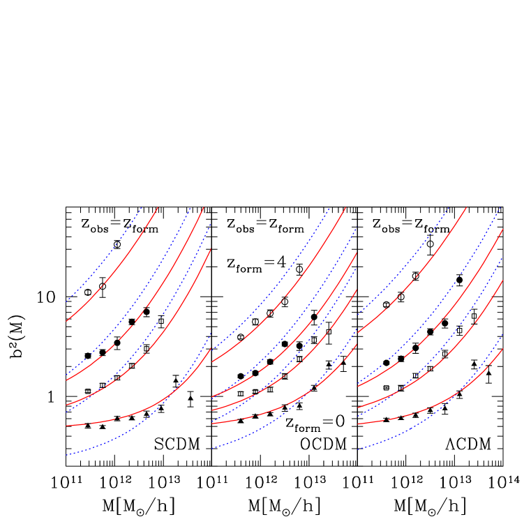
Figure 4 compares these predictions for the halo bias factors with measurements in simulations (from [254]). Note that more massive halos tend to be more biased, and that halos of the same mass were more strongly biased at high redshift than they are today. The solid and dotted lines show the predictions from equation (67) with equations (57) and (59) for the halo mass function, respectively. Figure 3 shows that equation (57) predicts too few massive halos; as a result, it predicts a larger bias factor for these massive halos than is seen in the simulations. Equation (59) provides an excellent fit to the halo mass function; the associated bias factors are also significantly more accurate.

Figure 4: Large scale bias relation between halos and mass (from [254]). Symbols show the bias factors at $z_{\rm obs}$ for objects which were identified as virialized halos at $z_{\rm form}=4$,2,1 and 0 (top to bottom in each panel). Dotted and solid lines show predictions based on the Press-Schechter and Sheth-Tormen mass functions.

The expressions above for the bias coefficients are obtained from our expression for the mean number of halos in cells $V$ which contain mass $M$. If the relation between $\delta_{\rm h}$ and $\delta$ is deterministic, that is, if the scatter around the mean number of halos at fixed $M$ and $V$ is small, then the distribution of halo overdensities is related to that of the dark matter overdensities by a non-linear transformation; the coefficients $b_{k}$ describe this relation. Thus, if the dark matter distribution at late times is obtained by a transformation of the initial distribution, then the halos are also related to the initial distribution through a non-linear transformation.

While a deterministic relation between $\delta_{\rm h}$ and $\delta$ is a reasonable approximation on large scales, on smaller scales the scatter is significant [190]. On small scales, the bias is both non-linear and stochastic. Accurate analytic models for this stochasticity are presented in [252, 35], but we will not need them for what follows. Also, ignored in what follows are: i) the deterministic bias coefficients $b_{k}(m,z_{1})$ which follow from the assumption that halos are associated with peaks in the initial density field [189]; ii) the deterministic bias coefficients which are motivated by perturbation theory rather than the spherical collapse model [36]. (Also, see [91] for a discussion of the relation between perturbation theory and the coefficients $a_{k}$ in the expressions above).

On large scales where deterministic biasing is a good approximation, the variance of halo counts in cells is

$$\Bigl{\langle}\delta_{\rm h}(m,z_{1}|M,V,z_{0})^{2}\Bigr{\rangle}=\Bigl{\langle}\left(\sum_{k>0}b_{k}(m,z_{1})\,\delta^{k}\right)^{2}\Bigr{\rangle}\approx b^{2}_{1}(m,z_{1})\,\Bigl{\langle}\delta^{2}\Bigr{\rangle}_{V}\,.$$ (71)

Thus, to describe the variance of the halos counts we must know the variance in the dark matter on the same scale: $\langle\delta^{2}\rangle_{V}$. On very large scales, it should be a good approximation to replace $\langle\delta^{2}\rangle$ by the linear theory estimate. On slightly smaller scales, it is better to use the perturbation theory estimates of [236]. Given these, the variance of halo counts in cells on large scales is straightforward to compute.

The higher order moments can also be estimated if the biasing is deterministic. This is because equation (66) allows one to write the higher order moments of the halo distribution, $\langle\delta_{\rm h}^{n}\rangle$, in terms of those of the dark matter, $\langle\delta^{n}\rangle$. Quasi-linear perturbation theory shows that $\langle\delta^{n}\rangle=S_{n}\,\langle\delta^{2}\rangle^{n-1}$ if $\langle\delta^{2}\rangle\ll 1$ (see equation 40). The $S_{n}$ are numerical coefficients which are approximately independent of scale over a range of scales on which $\langle\delta^{2}\rangle\ll 1$; for clustering from Gaussian initial conditions, the $S_{n}$ are given by equation (41). By keeping terms to consistent order, one can show that [88]

$$\Bigl{\langle}\delta_{\rm h}^{n}(m,z_{1}|M,V,z_{0})\Bigr{\rangle}=H_{n}\Bigl{\langle}\delta_{\rm h}^{2}(m,z_{1}|M,V,z_{0})\Bigr{\rangle}^{n-1},$$ (72)

where

$$H_{3} = b_{1}^{-1}(S_{3}+3c_{2}),\qquad H_{4}=b_{1}^{-2}(S_{4}+12c_{2}S_{3}+4c_{3}+12c_{2}^{2}),$$

$$H_{5} = b_{1}^{-3}\Bigl{[}S_{5}+20c_{2}S_{4}+15c_{2}S_{3}^{2}+(30c_{3}+120c_{2}^{2})S_{3}+5c_{4}+60c_{3}c_{2}+60c_{2}^{3}\Bigr{]},$$

$c_{k}=b_{k}/b_{1}$ and we have not bothered to write explicitly that $H_{n}$ depends on halo mass and on the cell size $V$.

Figure 5: Higher order moments of the halo distribution if the initial fluctuation spectrum is scale free and has slope $n=-1.5$. Dotted and solid curves show the result of assuming the halo mass function has the Press–Schechter and Sheth–Tormen forms.

The expressions above show that the distribution of halos depends explicitly on the distribution of mass. On large scales where the relation between halos and mass is deterministic, one might have thought that the linear theory description of the mass distribution can be used. For clustering from Gaussian initial conditions, however, linear theory itself predicts that $S_{n}=0$ for all $n>2$. Therefore, to describe the halo distribution, it is essential to go beyond linear theory to the quasi-linear perturbation theory.

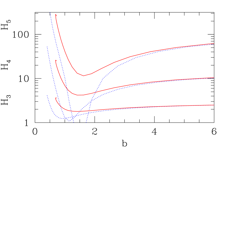
Figure 5 shows an example of how the first few $H_{n}$ depend on halo mass, parameterized by $b(m)$. Note that, in general, the less massive halos (those for which $b<1$) have larger values of $H_{n}$. This is a generic feature of halo models. At high masses ($b\gg 1$) both sets of curves asymptote to $H_{n}=n^{n-2}$.

Before moving on to the next subsection, consider some asymptotic properties of the $b_{k}$ in equation (67), and of the high order moments $H_{n}$ derived from them. For small halos ($\nu\ll 1$) identified at early times ($z_{1}\gg 1$), $b_{1}\approx 1$ and $b_{k}\approx 0$ for $k>1$. Therefore $H_{n}=S_{n}$ and such halos are not biased relative to mass. In contrast, when $\nu\gg 1$ and $z_{1}$ is not large, i.e. for massive halos identified at low redshift, $b_{k}=b_{1}^{k}$ for $k>1$. In this limit, the $H_{n}$ are independent of both $S_{n}$ and $a_{k}$. Therefore, the spatial distribution of these halos is determined completely by the statistical properties of the initial density field and are not modified by the dynamics of gravitational clustering. In the limit of $\nu\gg 1$, for an initially Gaussian random field, $H_{n}=n^{n-2}$; these are the coefficients of a Lognormal distribution which has small variance. This shows that the most massive halos, or the highest peaks in a Gaussian field, are not Gaussian distributed.

For small halos identified at low redshift ($\nu\ll 1$ and $z_{1}\ll 1$), $b_{1}\approx 1-1/\delta_{\rm sc}(z_{1})$ and $b_{k}\approx-k!(a_{k-1}+a_{k})/\delta_{\rm sc}(z_{1})$ for $k\geq 2$. In this case $H_{n}$ may depend significantly on the dynamical evolution of the underlying mass density field. The skewness of such halos, $H_{3}$, can be larger than $S_{3}$. On the other hand, for halos with $\nu=1$, the skewness is $H_{3}=S_{3}-6/\delta_{\rm sc}^{2}(z_{1})$, which is substantially smaller than $S_{3}$ unless $z_{1}$ is high.

The most important result of this subsection is that, in the limit in which biasing is deterministic, the bias parameters which relate the halo distribution to that of the mass are completely specified if the halo abundance, i.e., the halo mass function, is known. If perturbation theory is used to describe the distribution of the mass, then these bias parameters allow one to describe the distribution of the halos. The perturbation theory predictions and the halo mass function both depend on the shape of the initial power spectrum. Thus, in this model, the initial fluctuation spectrum is used to provide a complete description of halo biasing.

3.5 Halo density profiles

Secondary infall models of spherical collapse [82, 16] suggest that the density profile around the center of a collapsed halo depends on the initial density distribution of the region which collapsed. If halos are identified as peaks in the initial density field [143, 116], then massive halos correspond to higher peaks in the initial fluctuation field. The density run around a high peak is shallower than the run around a smaller peak [6]: high peaks are less centrally concentrated. Therefore one might reasonably expect massive virialized halos to also be less centrally concentrated than low mass halos. Such a trend is indeed found [198].

Figure 6: Distribution of dark matter around halo centers (from [198]). The density is in units of $10^{10}$ M${}_{\hbox{$\odot$}}$/kpc³ and radii are in kpc. Different panels show the density profile around the least and most massive halos in simulations of a wide variety of cosmological models and initial power spectra (labelled by the density parameter and spectral index). Arrows show the softening length; measurements on scales smaller than this are not reliable. Solid lines show the NFW fit to the density distribution is extremely accurate.

Figure 7: Mean concentration at fixed mass, $c_{\Delta}=r_{vir}/r_{s}$, for dark matter halos as a function of halo mass (from results presented in [78]). Different panels show the same cosmological models and power spectra as Figure 6.

Functions of the form

$$\rho(r|m)={\rho_{s}\over(r/r_{s})^{\alpha}(1+r/r_{s})^{\beta}}\quad{\rm or}\quad\rho(r|m)={\rho_{s}\over(r/r_{s})^{\alpha}[1+(r/r_{s})^{\beta}]}\,,$$ (73)

have been extensively studied as models of elliptical galaxies [111, 300]. Setting $(\alpha,\beta)=(1,3)$ and $(1,2)$ in the expression on the left gives the Hernquist [111] and NFW [198] profiles, whereas $(\alpha,\beta)=(3/2,3/2)$ in the expression on the right is the M99 profile [195].

Figure 8: Distribution of concentrations at fixed mass for dark matter halos fit to NFW profiles. Different symbols show results for halos in different mass bins. When normalized by the mean concentration in the bin, the distribution is well described by a log-normal function (equation 76). The pile up of halos at small values of the concentration is due to numerical resolution of the GIF simulations.

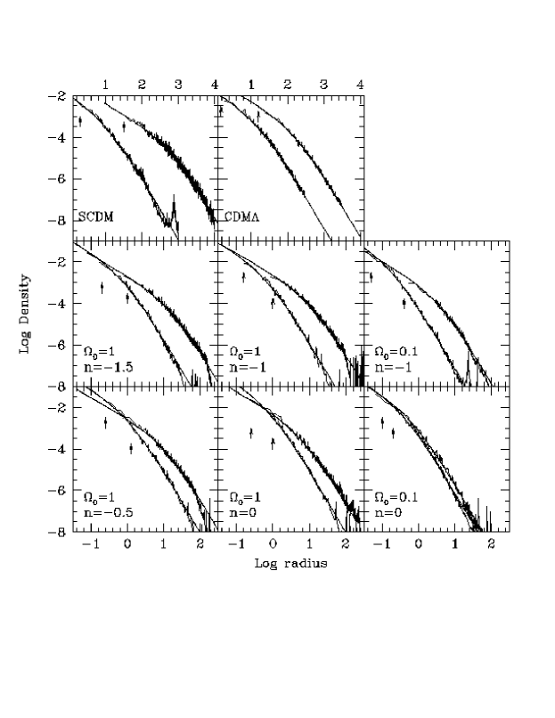
The NFW and M99 profiles provide very good descriptions of the density run around virialized halos in numerical simulations (figure 6). The two profiles differ on small scales, $r\ll r_{s}$, and whether one provides a better description of the simulations than the other is still being hotly debated. Both profiles are parameterized by $r_{s}$ and $\rho_{s}$, which define a scale radius and the density at that radius, respectively. Although they appear to provide a two-parameter fit, in practice, one finds an object of given mass $m$ and radius $r_{vir}$ in the simulations, and then finds that $r_{s}$ which provides the best fit to the density run. This is because the edge of the object is its virial radius $r_{vir}$, while the combination of $r_{s}$ and the mass determines the characteristic density, $\rho_{s}$, following

$$m\equiv\int_{0}^{r_{vir}}dr\,4\pi r^{2}\rho(r|m).$$ (74)

For the NFW and M99 profiles,

$$m=4\pi\rho_{s}r_{s}^{3}\,\left[\ln(1+c)-\frac{c}{1+c}\right]\quad{\rm and}\quad m=4\pi\rho_{s}r_{s}^{3}\,{2\ln(1+c^{3/2})\over 3},$$ (75)

where $c\equiv r_{vir}/r_{s}$ is known as the concentration parameter. Note that we have explicitly assumed that the halo profile is truncated at $r_{vir}$, even though formally, the NFW and M99 profiles extend to infinity. Because these profiles fall as $r^{-3}$ at large radii, the mass within them diverges logarithmically. Our decision to truncate the profile at the virial radius insures that the mass within the profile is the same as that which is described by the halo mass function discussed previously.

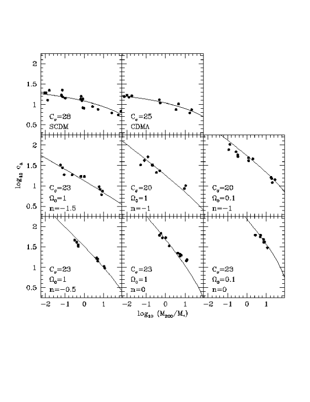
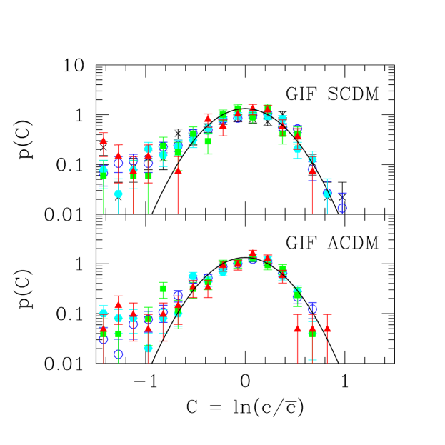
Since most of the mass is at radii much smaller than $r_{vir}$, the fitted value of $r_{s}$ is not very sensitive to the exact choice of the boundary $r_{vir}$. The simulations show that for halos of the same mass, there is a distribution of concentrations $c=r_{vir}/r_{s}$ which is well-fit by a log-normal distribution [138, 31]:

$$p(c|m,z)\,dc=\frac{d\ln c}{\sqrt{2\pi\sigma_{c}^{2}}}\,\exp\left[-\frac{\ln^{2}[c/\bar{c}(m,z)]}{2\,\sigma_{\ln c}^{2}}\right].$$ (76)

Although the mean concentration $\bar{c}(m,z)$ depends on halo mass, the width of the distribution does not. This is shown in Figure 8, which is taken from [256]. The Figure shows that the distribution of $c/\bar{c}$ is indeed well approximated by a log-normal function.

For the NFW profile,

$$\bar{c}(m,z)={9\over 1+z}\left[\frac{m}{m_{*}(z)}\right]^{-0.13}\qquad{\rm and}\qquad\sigma_{\ln c}\approx 0.25\,,$$ (77)

where $m_{*}(z)$ is characteristic mass scale at which $\nu(m,z)=1$. A useful approximation, due to [212], is that $\bar{c}[{\rm M99}]\approx(\bar{c}[{\rm NFW}]/1.7)^{0.9}$. Equation (77) quantifies the tendency for low mass halos to be more centrally concentrated, on average, than massive halos.

In what follows, it will be useful to have expressions for the normalized Fourier transform of the dark matter distribution within a halo of mass $m$:

$$u({\bf k}|m)={\int d^{3}{\bf x}\,\rho({\bf x}|m)\,e^{-i{\bf k}\cdot{\bf x}}\over\int d^{3}{\bf x}\,\rho({\bf x}|m)}.$$ (78)

For spherically symmetric profiles truncated at the virial radius, this becomes

$$u(k|m)=\int_{0}^{r_{vir}}dr\ 4\pi r^{2}\,{\sin kr\over kr}\ {\rho(r|m)\over m}.$$ (79)

Table 1 contains some $\rho(r|m)$ and $u(k|m)$ pairs which will be useful in what follows.

For the NFW profile,

$$u(k|m) = \frac{4\pi\rho_{s}r_{s}^{3}}{m}\,\Biggl{\{}\sin(kr_{s})\,\Bigl{[}{\rm Si}([1+c]kr_{s})-{\rm Si}(kr_{s})\Bigr{]}-\frac{\sin(ckr_{s})}{(1+c)kr_{s}}$$ (80)

$$\qquad\qquad\qquad+\cos(kr_{s})\,\Bigl{[}{\rm Ci}([1+c]kr_{s})-{\rm Ci}(kr_{s})\Bigr{]}\Biggr{\}}\,,$$

where the sine and cosine integrals are

$${\rm Ci}(x)=-\int_{x}^{\infty}\frac{\cos t}{t}\,dt\quad{\rm and}\quad{\rm Si}(x)=\int_{0}^{x}\frac{\sin t}{t}\,dt\,.$$ (81)

Figure 9 shows $u(k|m)$ as a function of $m$ for NFW halos. In general, the shape of the Fourier transform depends both on the halo concentration parameter, $c$, and the mass $m$. The figure shows a trend which is to all the profiles in Table 1: the small scale power is dominated by low mass halos.

Figure 9: Fourier transforms of normalized NFW profiles $u(k|m)$, for a variety of choices of halo mass, at the present time (redshift $z=0$). Equation (77) for the halo mass–concentration relation has been used. The curves show that the most massive halos contribute to the total power only at the largest scales, whereas smaller halos contribute power even at small scales.

There are no complete explanations for why the NFW or M99 profiles fit the dark matter density distribution of dark matter in numerical simulations, although there are reasonably successful models of why the concentrations depend on mass [198, 205, 288]. In the present context, the reason why they fit is of secondary importance; what is important is that these fits provide simple descriptions of the density run around a halo. In particular, what is important is that the density run around a dark matter halo depends mainly on its mass; though the density profile also depends on the concentration, the distribution of concentrations is determined by the mass.

Table 1: Density profiles and associated normalized Fourier transforms. Distances are in units of the scale radius: $x=r/r_{s}$, $c=r_{vir}/r_{s}$ and $\kappa=kr_{s}$, and, when truncated, the boundary of the halo is $r_{vir}$. The sine and cosine integrals are defined in the main text.

$\rho(x)$	range	$u(\kappa)$
$(2\pi)^{-3/2}\exp(-x^{2}/2)$		$\exp(-\kappa^{2}/2)$
$\exp(-x)/8\pi$		$(1+\kappa^{2})^{-2}$
$\exp(-x)/(4\pi x^{2})$		${\rm atan}(\kappa)/\kappa$
$x^{-2}(1+x^{2})^{-1}/(2\pi^{2})$		$[1-\exp(-\kappa)]/\kappa$
$3/(4\pi c^{3})$	$x\leq c$	$3\,[\sin(c\kappa)-c\kappa\,\cos(c\kappa)]/(c\kappa)^{3}$
$(4\pi c\,x^{2})^{-1}$	$x\leq c$	${\rm Si}(c\kappa)/c\kappa$
$x^{-1}(1+x)^{-2}$	$x\leq c$	Equation (80)

4 Halos and large scale structure

At this point, we have formulae for the abundance and spatial distribution of halos, as well as for the typical density run around a halo. This means that we are now in a position to construct the halo model. The treatment below will be completely general. To make the model quantitative, one simply inserts their favorite formulae for the halo profile, abundance and clustering (such as those presented in the previous section) into the expressions below.

The formalism written down by Neyman & Scott [199], which we are now in a position to consider in detail, had three drawbacks. First, it was phrased entirely in terms of discrete statistics; some work is required to translate it into the language of continuous density fields. Second, it was phrased entirely in terms of real coordinate space quantities. As we will see shortly, many of the formulae in the model involve convolutions which are considerably easier to perform in Fourier space. And, finally, the particular model they assumed for the clustering of halos was not very realistic.

Scherrer & Bertschinger [232] appear to have been the first to write the model for a continuous density field, using Fourier space quantities, in a formulation which allows one to incorporate more general and realistic halo–halo correlations into the model. It is this formulation which we describe below.

4.1 The two-point correlation function

In the model, all mass is bound up into halos which have a range of masses and density profiles. Therefore, the density at position ${{\mathbf{x}}}$ is given by summing up the contribution from each halo:

$$\rho({{\mathbf{x}}}) = \sum_{i}f_{i}({{\mathbf{x}}}-{{\mathbf{x}}}_{i})=\sum_{i}\rho({{\mathbf{x}}}-{{\mathbf{x}}}_{i}|m_{i})\equiv\sum_{i}m_{i}\ u({{\mathbf{x}}}-{{\mathbf{x}}}_{i}|m_{i})$$ (82)

$$= \sum_{i}\int dm\,d^{3}x^{\prime}\,\delta(m-m_{i})\,\delta^{3}({{\mathbf{x}}}^{\prime}-{{\mathbf{x}}}_{i})\ m\,u({{\mathbf{x}}}-{{\mathbf{x}}}^{\prime}|m),$$

where $f_{i}$ denotes the density profile of the $i$th halo which is assumed to be centered at ${{\mathbf{x}}}_{i}$. The second equality follows from assuming that the density run around a halo depends only on its mass; this profile shape is parameterized by $\rho$, which depends on the distance from the halo center and the mass of the halo. The third equality defines the normalized profile $u$, which is $\rho$ divided by the total mass contained in the profile: $\int d^{3}{{\mathbf{x}}}^{\prime}\,u({{\mathbf{x}}}-{{\mathbf{x}}}^{\prime}|m)=1$.

The number density of halos of mass $m$ is

$$\Bigl{\langle}\sum_{i}\delta(m-m_{i})\,\delta^{3}({{\mathbf{x}}}^{\prime}-{{\mathbf{x}}}_{i})\Bigr{\rangle}\equiv n(m),$$ (83)

where $\langle...\rangle$ denotes an ensemble average. The mean density is

$$\bar{\rho} = \Bigl{\langle}\rho({{\mathbf{x}}})\Bigr{\rangle}=\Bigl{\langle}\sum_{i}m_{i}\ u({{\mathbf{x}}}-{{\mathbf{x}}}_{i}|m_{i})\Bigr{\rangle}=\int dm\,n(m)m\int d^{3}{{\mathbf{x}}}^{\prime}\,u({{\mathbf{x}}}-{{\mathbf{x}}}^{\prime}|m)$$ (84)

$$= \int dm\,n(m)m,$$

where the ensemble average has been replaced by an average over the halo mass function $n(m)$ and an average over space.

The two-point correlation function is

$$\xi({{\mathbf{x}}}-{{\mathbf{x}}}^{\prime})=\xi^{1h}({{\mathbf{x}}}-{{\mathbf{x}}}^{\prime})+\xi^{2h}({{\mathbf{x}}}-{{\mathbf{x}}}^{\prime})$$ (85)

where

$$\xi^{1h}({{\mathbf{x}}}-{{\mathbf{x}}}^{\prime}) = \int dm\,{m^{2}\,n(m)\over\bar{\rho}^{2}}\int d^{3}{\bf y}\,u({\bf y}|m)\,u({\bf y}+{{\mathbf{x}}}-{{\mathbf{x}}}^{\prime}|m)$$

$$\xi^{2h}({{\mathbf{x}}}-{{\mathbf{x}}}^{\prime}) = \int dm_{1}\,{m_{1}\,n(m_{1})\over\bar{\rho}}\int dm_{2}\,{m_{2}\,n(m_{2})\over\bar{\rho}}\int d^{3}{{\mathbf{x}}}_{1}\,u({{\mathbf{x}}}-{{\mathbf{x}}}_{1}|m_{1})$$

$$\qquad\qquad\times\ \int d^{3}{{\mathbf{x}}}_{2}\,u({{\mathbf{x}}}^{\prime}-{{\mathbf{x}}}_{2}|m_{2})\ \xi_{hh}({{\mathbf{x}}}_{1}-{{\mathbf{x}}}_{2}|m_{1},m_{2})\,;$$

the first term describes the case in which the two contributions to the density are from the same halo, and the second term represents the case in which the two contributions are from different halos. Both terms require knowledge of how the halo abundance and density profile depend on mass. The second term also requires knowledge of $\xi_{hh}({{\mathbf{x}}}-{{\mathbf{x}}}^{\prime}|m_{1},m_{2})$, the two-point correlation function of halos of mass $m_{1}$ and $m_{2}$.

The first term is relatively straightforward to compute: it is just the convolution of two similar profiles of shape $u(r|m)$, weighted by the total number density of pairs contributed by halos of mass $m$. This term was studied in the 1970’s, before numerical simulations had provided accurate models of the halo abundances and density profiles [215, 184]. The more realistic values of these inputs were first used to model this term some twenty years later [250].

The second term is more complicated. If $u_{1}$ and $u_{2}$ were extremely sharply peaked, then we could replace them with delta functions; the integrals over ${{\bf x}_{1}}$ and ${{\bf x}_{2}}$ would yield $\xi_{hh}({{\mathbf{x}}}-{{\mathbf{x}}}^{\prime}|m_{1},m_{2})$. Writing ${{\mathbf{x}}}_{1}-{{\mathbf{x}}}_{2}=({{\mathbf{x}}}-{{\mathbf{x}}}^{\prime})+({{\mathbf{x}}}^{\prime}-{{\mathbf{x}}}_{2})-({{\mathbf{x}}}-{{\mathbf{x}}}_{1})$, shows that this should also be a reasonable approximation if $\xi_{hh}(r|m_{1},m_{2})$ varies slowly on scales which are larger than the typical extent of a halo. Following the discussion in the previous section with respect to halo bias, on large scales where biasing is deterministic,

$$\xi_{hh}(r|m_{1},m_{2})\approx b(m_{1})\,b(m_{2})\ \xi(r)$$ (86)

Now $\xi(r)$ can be taken outside of the integrals over $m_{1}$ and $m_{2}$, making the two integrals separable. The consistency relations (equation 70) show that each integral equals unity. Thus, on scales which are much larger than the typical halo $\xi^{2h}(r)\approx\xi(r)$. However, on large scales, $\xi(r)\approx\xi^{\rm lin}(r)$, and so the two-halo term is really very simple: $\xi^{2h}(r)\approx\xi^{\rm lin}(r)$.

Setting $\xi_{hh}(r|m_{1},m_{2})\approx b(m_{1})\,b(m_{2})\,\xi(r)$ will overestimate the correct value on intermediate scales. Furthermore, on small scales the halo-halo correlation function must eventually turn over (halos are spatially exclusive—so each halo is like a small hard sphere); assuming that it scales like $\xi(r)$ is a gross overestimate. Using $\xi_{hh}(r|m_{1},m_{2})\approx b(m_{1})\,b(m_{2})\ \xi^{\rm lin}(r)$, i.e., using the linear, rather than the non-linear correlation function, even on the smallest scales, is a crude but convenient way of accounting for this overestimate. Although the results of [252] allow one to account for this more precisely, it turns out that great accuracy is not really needed since, on small scales, the correlation function is determined almost entirely by the one-halo term anyway. Although almost all work to date uses this approximation, it is important to bear in mind that it’s form is motivated primarily by convenience. For example, if volume exclusion effects are only important on very small scales, then setting $\xi(r)\approx\xi^{\rm 1-loop}(r)$ rather than $\xi^{\rm lin}(r)$, i.e., using the one–loop perturbation theory approximation rather than the simpler linear theory estimate, may provide a better approximation.

Because the model correlation function involves convolutions, it is much easier to work in Fourier space: the convolutions of the real-space density profiles become simple multiplications of the Fourier transforms of the halo profiles. Thus, we can write the dark matter power spectrum as

$$P(k) = P^{1h}(k)+P^{2h}(k),\qquad{\rm where}$$

$$P^{1h}(k) = \int dm\,n(m)\left(\frac{m}{\bar{\rho}}\right)^{2}\,|u(k|m)|^{2}$$

$$P^{2h}(k) = \int dm_{1}\,n(m_{1})\left(\frac{m_{1}}{\bar{\rho}}\right)\,u(k|m_{1})$$

$$\quad\quad\int dm_{2}\,n(m_{2})\left(\frac{m_{2}}{\bar{\rho}}\right)\,u(k|m_{2})\,P_{hh}(k|m_{1},m_{2})\,.$$

Here, $u(k|m)$ is the Fourier transform of the dark matter distribution within a halo of mass $m$ (equation 79) and $P_{hh}(k|m_{1},m_{2})$ represents the power spectrum of halos of mass $m_{1}$ and $m_{2}$. Following the discussion of the halo–halo correlation function (equation 86), we approximate this by

$$P_{hh}(k|m_{1},m_{2})\approx\prod_{i=1}^{2}b_{i}(m_{i})P^{\rm lin}(k)\\$$

bearing in mind that the one-loop perturbation theory estimate may be more accurate than $P^{\rm lin}(k)$.

4.2 Higher-order correlations

Expressions for the higher order correlations may be derived similarly. However, they involve multiple convolutions of halo profiles. This is why it is much easier to work in Fourier space: the convolutions of the real-space density profiles become simple multiplications of the Fourier transforms of the halo profiles. Similarly, the three-point and four-point correlations include terms which describe the three and four point halo power spectra. The bi- and tri- spectra of the halos are

$$B_{hhh}({\bf k}_{1},{\bf k}_{2},{\bf k}_{3};m_{1},m_{2},m_{3}) = \prod_{i=1}^{3}b_{i}(m_{i})\Biggl{[}B^{\rm lin}({\bf k}_{1},{\bf k}_{2},{\bf k}_{3})$$

$$\qquad+\frac{b_{2}(m_{3})}{b_{1}(m_{3})}P^{\rm lin}(k_{1})P^{\rm lin}(k_{2})\Biggr{]}\,,$$

$$T_{hhhh}({\bf k}_{1},{\bf k}_{2},{\bf k}_{3},{\bf k}_{4};m_{1},m_{2},m_{3},m_{4}) = \prod_{i=1}^{4}b_{i}(m_{i})\Biggl{[}T^{\rm lin}({\bf k}_{1},{\bf k}_{2},{\bf k}_{3},{\bf k}_{4})$$

$$\quad+\frac{b_{2}(m_{4})}{b_{1}(m_{4})}P^{\rm lin}(k_{1})P^{\rm lin}(k_{2})P^{\rm lin}(k_{3})\Biggr{]}\,.$$

Notice that these require the power, bi- and trispectra of the mass, as well as mass-dependent $i$th-order bias coefficients $b_{i}(m)$. Whereas $P$, $B$ and $T$ come from perturbation theory (§ 2.2), the bias coefficients are from the non-linear spherical or ellipsoidal collapse models and are given in § 3.3.

Using this information, we can write the dark matter bispectrum as

$$B_{123}=B^{1h}+B^{2h}+B^{3h}\,,$$ (89)

where,

$$B^{1h}=\int dm\,n(m)\left(\frac{m}{\bar{\rho}}\right)^{3}\ \prod_{i=1}^{3}u({\vec{k}}_{i}|m)$$

$$B^{2h}=\Big{[}\int dm_{1}\,n(m_{1})\left(\frac{m_{1}}{\bar{\rho}}\right)\,u(k_{1}|m_{1})\int dm_{2}\,n(m_{2})\left(\frac{m_{2}}{\bar{\rho}}\right)^{2}\,u(k_{2}|m_{2})u(k_{3}|m_{2})$$

$$\quad\quad\times P_{hh}(k_{1}|m_{1},m_{2})+{\rm cyc.}\Big{]}$$

$$B^{3h}=\left[\prod_{i=1}^{3}\int dm_{i}\,u(k_{i}|m_{i})n(m_{i})\left(\frac{m_{i}}{\bar{\rho}}\right)\right]B_{hhh}^{123}(m_{1},m_{2},m_{3})\,,$$

(90)

where $B_{hhh}^{123}(m_{1},m_{2},m_{3})\equiv B_{hhh}(k_{1},k_{2},k_{3}|m_{1},m_{2},m_{3})$ and denotes the bispectrum of halos of mass $m_{1},m_{2}$ and $m_{3}$.

Finally, the connected part of the trispectrum can be written as the sum of four terms

$$T_{1234}=T^{1h}+T^{2h}+T^{3h}+T^{4h}\,,$$ (91)

where

$$T^{1h}=\int dm\,n(m)\left(\frac{m}{\bar{\rho}}\right)^{4}\ \prod_{i=1}^{4}u({\vec{k}}_{i}|m)$$ (92)

$$T^{2h}=\Big{[}\int dm_{1}\,n(m_{1})\left(\frac{m_{1}}{\bar{\rho}}\right)\,u(k_{1}|m_{1})\int dm_{2}\,n(m_{2})\left(\frac{m_{2}}{\bar{\rho}}\right)^{3}\,$$

$$\quad\quad\times u(k_{2}|m_{2})u(k_{3}|m_{2})u(k_{4}|m_{2})P_{hh}(k_{1}|m_{1},m_{2})+{\rm cyc.}\Big{]}$$

$$+ \Big{[}\int dm_{1}\,n(m_{1})\left(\frac{m_{1}}{\bar{\rho}}\right)^{2}\,u(k_{1}|m_{1})u(k_{2}|m_{2})\int dm_{2}\,n(m_{2})\left(\frac{m_{2}}{\bar{\rho}}\right)^{2}\,u(k_{3}|m_{2})u(k_{4}|m_{2})$$

$$\quad\quad\times P_{hh}(|{\bf k}_{1}+{\bf k}_{2}||m_{1},m_{2})+{\rm cyc.}\Big{]}$$

$$T^{3h}=\int dm_{1}\,n(m_{1})\left(\frac{m_{1}}{\bar{\rho}}\right)\,u(k_{1}|m_{1})\int dm_{2}\,n(m_{2})\left(\frac{m_{2}}{\bar{\rho}}\right)\,u(k_{2}|m_{2})$$

$$\quad\quad\times\int dm_{3}\,n(m_{3})\left(\frac{m_{3}}{\bar{\rho}}\right)^{2}\,u(k_{3}|m_{3})u(k_{4}|m_{3})B_{hhh}({\bf k}_{1},{\bf k}_{2},{\bf k}_{3}+{\bf k}_{4}|m_{1},m_{2},m_{3})$$

$$T^{4h}=\left[\prod_{i=1}^{4}\int dm_{i}\,u(k_{i}|m_{i})n(m_{i})\left(\frac{m_{i}}{\bar{\rho}}\right)\right]T_{hhhh}^{1234}(m_{1},m_{2},m_{3},m_{4}).$$

For simplicity, we reduce the notation related to integrals over the Fourier transform of halo profiles and write the power spectrum,

$$P(k)=P^{1h}(k)+P^{2h}(k)$$

$$P^{1h}(k)=M_{02}(k,k)$$

$$P^{2h}=P^{\rm lin}(k)\left[M_{11}(k)\right]^{2}\,,$$ (93)

bispectrum,

$$B_{123}=B^{1h}+B^{2h}+B^{3h}$$

$$B^{1h}=M_{03}(k_{1},k_{2},k_{3})$$

$$B^{2h}=M_{11}(k_{1})M_{12}(k_{2},k_{3})P^{\rm lin}(k_{1})+{\rm cyc.}$$

$$B^{3h}=\left[\prod_{i=1}^{3}M_{11}(k_{i})\right]B^{\rm lin}_{123}+M_{11}(k_{1})M_{11}(k_{2})M_{21}(k_{3})P^{\rm lin}(k_{1})P^{\rm lin}(k_{2})+{\rm cyc.}\,,$$

(94)

and trispectrum,

$$T_{1234}=T^{1h}+T^{2h}+T^{3h}+T^{4h}$$

$$T^{1h}=M_{04}(k_{1},k_{2},k_{3},k_{4})$$

$$T^{2h}=\Big{[}M_{11}(k_{1})M_{13}(k_{2},k_{3},k_{4})P^{\rm lin}(k_{1})+{\rm cyc.}\Big{]}$$

$$\quad\quad+\Big{[}M_{12}(k_{1},k_{2})M_{12}(k_{3},k_{4})P^{\rm lin}(|{\bf k}_{1}+{\bf k}_{2}|)+{\rm cyc.}\Big{]}$$

$$T^{3h}=M_{11}(k_{1})M_{11}(k_{2})M_{12}(k_{3},k_{4})B^{\rm lin}({\bf k}_{1},{\bf k}_{2},{\bf k}_{3}+{\bf k}_{4})$$

$$\quad\quad+\Big{[}M_{11}(k_{1})M_{11}(k_{2})M_{22}(k_{3},k_{4})P^{\rm lin}(k_{1})P^{\rm lin}(k_{2})+{\rm cyc.}\Big{]}$$

$$T^{4h}=\left[\prod_{i=1}^{4}M_{11}(k_{i})\right]T^{\rm lin}_{1234}$$

$$\quad+M_{11}(k_{1})M_{11}(k_{2})M_{11}(k_{3})M_{21}(k_{4})P^{\rm lin}(k_{1})P^{\rm lin}(k_{2})P^{\rm lin}(k_{3})+{\rm cyc.}\,.$$ (95)

Here, $b_{0}\equiv 1$ and

$$M_{ij}(k_{1},\ldots,k_{j})\equiv\int dmn(m)\left(\frac{m}{\bar{\rho}}\right)^{j}b_{i}(m)[u(k_{1}|m)\ldots u(k_{j}|m)]\,,\\$$

with the three-dimensional Fourier transform of the halo density distribution, $u(k|m)$, following equation (79).

The one-point moments, smoothed on scale $R$, can also be obtained by an integral with the appropriate window function $W(kR)$. In the case of variance,

$$\sigma^{2}(R) = \int\frac{k^{2}dk}{2\pi^{2}}P(k)|W(kR)|^{2}$$ (96)

$$= \int\frac{k^{2}dk}{2\pi^{2}}P^{\rm lin}(k)\left[M_{11}(k)\right]^{2}|W(kR)|^{2}+\int\frac{k^{2}dk}{2\pi^{2}}M_{02}(k,k)|W(kR)|^{2}$$

$$\approx \sigma^{2}_{\rm lin}(R)+\int dmn(m)\left(\frac{m}{\bar{\rho}}\right)^{2}\overline{u^{2}}(R|m)\,$$

where

$$\overline{u^{n}}(R|m)=\int\frac{k^{2}dk}{2\pi^{2}}u^{n}(k|m)|W(kR)|^{2}\,.$$ (97)

In simplifying, we have written the fully non-linear power spectrum of the density field in terms of the halo model (equation 93) and taken the large-scale limit $M_{11}\approx 1$. This is a reasonable approximation because of the consistency conditions (equation 70). Here, $\sigma^{2}_{\rm lin}(R)$ follows from equation (58). With similar approximations, we can derive higher-order connect moments (see [236] for details).

With the same general integral defined in [236],

$$A_{ij}(R)\equiv\int dmn(m)\left(\frac{m}{\bar{\rho}}\right)^{2}b_{i}(m)\overline{u^{2}}(R|m)\overline{u^{j}}(R|m)\,,$$ (98)

we can write the one point moments as

$$\langle\delta^{2}\rangle\equiv\sigma^{2}=\sigma_{\rm lin}^{2}+A_{00}$$

$$\langle\delta^{3}\rangle=S_{3}^{\rm lin}\sigma_{\rm lin}^{4}+3\sigma_{\rm lin}^{2}A_{10}+A_{01}$$

$$\langle\delta^{4}\rangle_{c}=S_{4}^{\rm lin}\sigma_{\rm lin}^{6}+6\frac{S_{3}^{\rm lin}}{3}\sigma_{\rm lin}^{4}A_{10}+7\frac{4\sigma_{\rm lin}^{2}}{7}A_{11}+A_{02}$$

$$\langle\delta^{5}\rangle_{c}=S_{5}^{\rm lin}\sigma_{\rm lin}^{8}+10\frac{S_{4}^{\rm lin}}{16}\sigma_{\rm lin}^{6}A_{10}+25\frac{3S_{3}^{\rm lin}}{5}\sigma_{\rm lin}^{4}A_{11}+15\frac{\sigma_{\rm lin}^{2}}{3}A_{12}+A_{03}\,,$$

(99)

where the terms in $\langle\delta^{n}\rangle_{c}$ are ordered from $n$-halo to 1-halo contributions. The coefficient of an $m$-halo contribution to $\langle\delta^{n}\rangle_{c}$ is given by $s(n,m)$ (e.g. $6$ and $7$ in the second and third terms of equation 99), the Stirling number of second kind, which is the number of ways of putting $n$ distinguishable objects ($\delta$) into $m$ cells (halos), with no cells empty [232].

In general, we can write the $n$th moment as

$$\langle\delta^{n}\rangle_{c}=S_{n}^{\rm PT}\sigma^{2(n-1)}_{L}+\sum_{m=2}^{n-1}s(n,m)\ \alpha_{nm}S_{m}^{\rm PT}\ \sigma^{2(m-1)}_{L}A_{1n-m-1}+A_{0n-2},$$ (100)

where the first term in equation (100) represents the $n-$halo term, the second term is the contribution from $m$-halo terms, and the last term is the 1-halo term. The coefficients $\alpha_{nm}$ measure how many of the terms contribute as $A_{1n-m-1}$, with the other contributions being subdominant. For example, in equation (99), the 2-halo term has a total contribution of 7 terms, 4 of them contain 3 particles in one halo and 1 in the other, and 3 of them contain 2 particles in each. The factor $4/7$ is included to take into account that the $3-1$ amplitude dominates over the $2-2$ amplitude. Note that in these results, we neglected all contributions from the non-linear biasing parameters in view of the consistency conditions given in equation (70). The $S_{n}^{\rm PT}$ were defined in equation (41).

4.3 An illustrative analytic example

To introduce the general behavior of the halo based predictions, we first consider a simple illustrative example. We assume that the initial spectrum of the density fluctuation field is $P_{0}(k)=A/k^{3/2}$. This is not a bad approximation to the shape of the power spectrum on cluster-like scales in CDM models. If we set $\Delta^{2}_{0}(k)\equiv k^{3}\,P_{0}(k)/(2\pi^{2})$ then the variance on scale $R$ is

$$\sigma^{2}(R)=\int{{\rm d}k\over k}\Delta^{2}_{0}(k)\,W^{2}_{\rm TH}(kR)={16\sqrt{\pi}\over 15}{A\over 2\pi^{2}}\,{R^{-3/2}}.$$ (101)

Setting $\sigma(R_{*})\equiv\delta_{\rm sc}$ means

$$\Delta^{2}_{0}(k)={15\,\delta_{\rm sc}^{2}\over 16\sqrt{\pi}}\,(kR_{*})^{3/2}.$$ (102)

We will approximate the fraction of mass in virialized halos of mass $m$ using equation (57):

$$f(m)\,{\rm d}m={mn(m)\,{\rm d}m\over\bar{\rho}}={{\rm d}\nu\over\nu}\,\sqrt{\nu\over 2\pi}\,\exp\left(-{\nu\over 2}\right),$$

where $\nu\equiv\delta^{2}_{\rm sc}/\sigma^{2}(m)=(m/m_{*})^{1/2}$ and $m_{*}=4\pi R_{*}^{3}\bar{\rho}/3$. We will assume that the density run around the center of a virialized halo scales as

$${\rho(r|m)\over\bar{\rho}}={2\Delta_{\rm nl}\over 3\pi}\,c^{3}(m)\,{y^{-2}\over 1+y^{2}},$$ (103)

when $\bar{\rho}$ is the background density, $y=r/r_{s}$, $c=r_{vir}/r_{s}$, $\Delta_{\rm nl}=(R/r_{vir})^{3}$, and $m/\bar{\rho}=4\pi R^{3}/3$. Here $R$ is the initial size of the halo, $r_{vir}$ is the virial size, and $r_{s}$ is the core radius. Since the profile falls more steeply than $r^{-3}$ at large $r$, the total mass is finite: $4\pi\int{\rm d}r\ r^{2}\rho(r|m)=m$. We will assume that the core radius depends on halo mass: $c(m)=c_{*}\,(m_{*}/m)^{\gamma}$.

The normalized Fourier transform of this profile is

$$u(k|m) = {\int{\rm d}r\ r^{2}\rho(r|m)\,\sin(kr)/(kr)\over\int{\rm d}r\ r^{2}\rho(r|m)}={1-{\rm e}^{-kr_{s}}\over kr_{s}},$$

$${\rm where} kr_{s}={kR_{*}\over\Delta^{1/3}_{\rm nl}c_{*}}\left({m\over m_{*}}\right)^{\gamma+1/3}\equiv\kappa\,\left({m\over m_{*}}\right)^{\gamma+1/3}.$$ (104)

Note that at large $k$, $u(k|m)$ decreases as $1/k$.

If we set $\gamma=1/6$ (so more massive halos are less concentrated), then $kr_{s}=\kappa\nu$, and the integrals over the mass function which define the power spectrum can be done analytically. For example, the contribution to the power from particles which are in the same halo is

$$\Delta^{2}_{1h}(k)=\int{\rm d}m\,{m^{2}n(m)\over\bar{\rho}^{2}}\,|u(k|m)^{2}|={2\,\Delta_{\rm nl}\over 3\pi}\,c_{*}^{3}\,\kappa\left(1+{1\over\sqrt{1+4\kappa}}-{2\over\sqrt{1+2\kappa}}\right),$$

and the contribution from pairs in separate halos is

$$\Delta^{2}_{2h}(k)=B^{2}(k)\,\Delta^{2}_{0}(k)=B^{2}(k)\,{15\,\delta_{\rm sc}^{2}\over 16\sqrt{\pi}}\,(\Delta_{\rm nl}^{1/3}c_{*})^{3/2}\,\kappa^{3/2},$$

where

$$B(k)={1\over\kappa}\Biggl{[}{2\over\delta_{\rm sc}}-1+\sqrt{1+2\kappa}\left(1-{1\over\delta_{\rm sc}}\right)-{1/\delta_{\rm sc}\over\sqrt{1+2\kappa}}\Biggr{]}.$$

Here $B(k)\equiv\int{\rm d}m\,[mn(m)/\bar{\rho}]\,b(m)\,u(k|m)$ and we have used the fact that, if the mass function is given by equation (57), then $b(m)=1+(\nu-1)/\delta_{\rm sc}$ from equation (65).

At small $\kappa$, the one-halo term is $2\Delta_{\rm nl}\,c^{3}_{*}/\pi$ times $\kappa^{3}$, whereas the two-halo term is $\Delta^{2}_{0}(k)$ times $B^{2}(k)\to 1-(2/\delta_{\rm sc}+1)\kappa$; the effect is to multiply the linear spectrum by a $k$ dependent factor which is less than unity. Thus, at small $k$ most of the power comes from the two-halo term. At large $k$, the two-halo term is $2(1-1/\delta_{\rm sc})^{2}/\kappa$ times the linear spectrum, so it grows as $\kappa^{1/2}$. On the other hand, the one-halo term is $2\Delta_{\rm nl}c^{3}_{*}/3\pi$ times $\kappa$. Thus, the power on small scales is dominated by the one-halo term.

If, on the other hand, $\gamma=-1/3$ (so more massive halos are more concentrated, unlike numerically simulated halos), then $\kappa=kr_{s}=kR_{*}/(c_{*}\Delta_{\rm nl}^{1/3})$ is independent of $m$, and so $u(k|m)$ is also independent of $m$. Since $\int{\rm d}m\ (m/\bar{\rho})^{2}\,n(m)=3\,(m_{*}/\bar{\rho})$, the two power spectrum terms are

$$\Delta^{2}_{1h}(k)={2\Delta_{\rm nl}\over\pi}\,c_{*}^{3}\,\kappa^{3}\left({1-{\rm e}^{-\kappa}\over\kappa}\right)^{2}\ {\rm and}\ \ \Delta^{2}_{2h}(k)=\left({1-{\rm e}^{-\kappa}\over\kappa}\right)^{2}\Delta^{2}_{0}(k).$$

This shows how the variation of the central concentration with halo mass changes the contribution to the total power from the two terms. In addition, changing the halo mass function would obviously change the final answer. And, for $\gamma=-1/3$, changing the initial power spectrum only changes the prefactor in front of $\Delta^{2}_{1h}(k)$. The prefactor in front of $\Delta^{2}_{2h}(k)$ is unaffected, though, of course, $\Delta^{2}_{0}(k)$ has been changed.

4.4 Compensated profiles

This section considers density profiles which are ‘compensated’; these are combinations of over- and under-dense perturbations, normalized so that the mass in each of the two components is the same. The reason for considering such profiles is to illustrate a curious feature of the halo model: when only positive perturbations are present, then, as $k\to 0$, the single halo contribution to the power tends to a constant:

$$P^{1h}(k\to 0)\to\int dm\,n(m)\,\left({m^{2}\over\bar{\rho}^{2}}\right)$$ (105)

In CDM–like spectra, the linear power-spectrum is $\propto k$ at small $k$, so that the single halo term eventually dominates the power. This problem is also present in the higher order statistics such as the bi- and trispectra. For the power spectrum, this constant is like a mean square halo mass, so that this excess large scale power resembles a shot-noise like contribution. This suggests that it must be subtracted–off by hand. However, subtracting the same constant at all $k$ is not a completely satisfactory solution, because the power at sufficiently large $k$ can be very small, in which case subtracting off $P^{1h}(k=0)$ might lead to negative power at large $k$. The compensated profile model is designed so that the one-halo term is well behaved at small $k$. On the other hand, as we show, compensated models suffer from another problem: they have no power on large scales!

Consider the correlation function which arises from a random, Poisson, distribution of density perturbations, in which all perturbations are assumed to be identical. We will consider what happens when we allow perturbations to have a range of sizes later, and correlations between perturbations will be included last. The density at a distance $r$ from a compensated perturbation can be written as the sum of two terms:

$$\rho(r)=\rho_{+}(r)+\rho_{-}(r).$$ (106)

So that we have a concrete model to work with, we will assume that

$${\rho_{+}(x)\over\bar{\rho}}=a\,\exp\left({-x^{2}\over 2\sigma_{+}^{2}}\right)\qquad{\rm and}\qquad{\rho_{-}(x)\over\bar{\rho}}=1-\exp\left({-x^{2}\over 2\sigma_{-}^{2}}\right),$$ (107)

where $\bar{\rho}$ denotes the mean density of the background in which these perturbations are embedded. (The Gaussian is a convenient choice because it is a monotonic function for which the necessary integrals are simple.) We will require $a>1$, so that the positive perturbation is denser than the background. We will discuss the scales $\sigma_{+}$ and $\sigma_{-}$ of the two perturbations shortly. For now, note that the negative perturbation is bounded between zero and one: $\rho_{-}(x)$ is always less than the mean density. The reason for this is that we are imagining that the perturbation can be thought of as an initially uniform density region of size $\sigma_{-}$ from which mass has been scooped out according to $\rho_{-}(x)$, and replaced by mass which is distributed as $\rho_{+}(x)$. The total density fluctuation is

$$\delta(x)\equiv{\rho(x)\over\bar{\rho}}-1=a\,\exp\left(-x^{2}\over 2\sigma_{+}^{2}\right)-\exp\left(-x^{2}\over 2\sigma_{-}^{2}\right).$$ (108)

The integral of $\delta$ over all space is

$$g\equiv 4\pi\int_{0}^{\infty}{\rm d}x\ x^{2}\,\delta(x)=(2\pi)^{3/2}\,\Bigl{(}a\,\sigma_{+}^{3}-\sigma_{-}^{3}\Bigr{)}\,,$$ (109)

and depends on the amplitudes and scales of the positive and negative perturbations.

If we set

$$\sigma_{-}=a^{1/3}\,\sigma_{+}$$ (110)

then $g=0$. This corresponds to the statement that the positive perturbation contributes exactly the same amount of mass which the negative perturbation removed. The only difference is that the mass has been redistributed into the form $\rho_{+}(x)$. It is in this sense that the profiles are compensated.

We can build a toy model of evolution from this by defining $\sigma_{+}(t)/\sigma_{-}\equiv R(t)$. We will imagine that, at some initial time, $R(t)\approx 1$, and that it decreases thereafter. This is supposed to represent the fact that gravity is an attractive force, so the mass which was initially contained with $\sigma_{-}$ is later contained within the smaller region $\sigma_{+}$. If mass is conserved as $\sigma_{+}$ shrinks (equation 110), then it must be that $a(t)=R(t)^{-1}$. Thus, the amplitude $a$ is related to the ratio of the initial and final sizes of $\sigma_{+}$. The fact that $R(t)\approx 1$ initially reflects the assumption that the initial density field was uniform. Today, the mass is in dense clumps—the positive perturbations. Each positive perturbation assembled its mass from a larger region in the initial conditions. Our particular choice of setting $g$ to zero comes from requiring that all the mass in the positive perturbation came from the negative one.

Note that we haven’t yet specified the exact form for the evolution of the profile, $R(t)$. Independent of this evolution, we can use the formalism in [183] to compute the correlation functions as a function of given $t$. The correlation function is the number density of profiles, $\eta$, times the convolution of such a profile with itself, $\lambda(r)$. Since all the mass is in the positive perturbations, and each positive perturbation contains mass $m=(2\pi)^{3/2}\,\bar{\rho}\,\sigma_{-}^{3}$, we can set $\eta=\bar{\rho}/m$. In our compensated halo model, $\lambda$ is the sum of three terms:

$$\lambda(r)=\lambda_{++}(r)+\lambda_{--}(r)-2\lambda_{+-}(r),$$ (111)

where $\lambda_{++}$,$\lambda_{--}$, and $\lambda_{+-}$, denote the various types of convolutions. For the Gaussian profiles we are considering here,

$$\lambda_{++}(r) = a^{2}\,\pi^{3/2}\,\sigma_{+}^{3}\,\exp\left({-r^{2}\over 4\sigma_{+}^{2}}\right),\qquad\lambda_{--}(r)=\pi^{3/2}\,\sigma_{-}^{3}\,\exp\left({-r^{2}\over 4\sigma_{-}^{2}}\right),$$

$$\lambda_{+-}(r) = a\,\pi^{3/2}\,\left(2\,\sigma_{+}^{2}\,\sigma_{-}^{2}\over\sigma_{+}^{2}+\sigma_{-}^{2}\right)^{3/2}\,\exp\left({-r^{2}/2\over\sigma_{+}^{2}+\sigma_{-}^{2}}\right).$$ (112)

Inserting equation (110) makes the factors in front of the exponentials resemble each other more closely.

It is a simple matter to verify that these compensated profiles satisfy the integral constraint:

$$\eta\,4\pi\int_{0}^{\infty}{\rm d}r\ r^{2}\,\lambda(r)=0.$$ (113)

If the correlation function were always positive, this integral constraint would not be satisfied. Because of the minus sign in equation (111) above, the correlation function in compensated halo models can be negative on large scales.

The power spectrum is obtained by Fourier-transforming the correlation function. Since the Fourier transform of a Gaussian is a Gaussian, equation (112) shows that, in these compensated models, the power spectrum is the sum of three Gaussians:

$$P(k) = {1\over 2\pi^{2}}\int{\rm d}r\ r^{2}\,\eta\lambda(r)\,{\sin kr\over kr}$$ (114)

$$= \eta\,(a\,\sigma_{+}^{3})^{2}\,\left({\rm e}^{-k^{2}\sigma_{+}^{2}}+{\rm e}^{-k^{2}\sigma_{-}^{2}}-2\,{\rm e}^{-k^{2}\sigma_{+}^{2}/2}{\rm e}^{-k^{2}\sigma_{-}^{2}/2}\right).$$

The form of this expression is easily understood, since convolutions in real space are multiplications in Fourier space such that the power spectrum is simply a sum of products of Gaussians. Indeed, if we let $U(k)$ and $W(k)$ denote the Fourier transforms of the positive and negative perturbations, then

$$P(k)=\Bigl{[}U(k)-W(k)\Bigr{]}^{2}.$$ (115)

It is interesting to compare this expression with the case of a positive perturbation only. In this case, $\lambda=\lambda_{++}$, and $P(k)=U(k)^{2}$. Since $\lambda_{++}\geq 0$ always, such a model does not satisfy the integral constraint. Analogously, uncompensated profiles have $P(k)\to$ constant at small $k$. If one thinks of the compensated profile as providing a correction factor to the power spectrum of positive perturbations, then the expression above shows that this correction is $k$ dependent: simply subtracting-off a constant term from $U(k)$ is incorrect. In the compensated Gaussian model above, $W(k)\to 0$ at large $k$, so $P(k)\to U(k)$ on small scales. However, $P(k)\to 0$ at small $k$—there is no power on large scales.

Figure 10: Density profiles and correlation functions associated with uncompensated (dashed) and compensated (solid) Gaussian perturbations. The correlation function $\lambda$ is negative for $r/\sigma_{+}$ in the range $3-15$ or so, so we have plotted $|\lambda|$ instead.

Fig. 10 shows all this explicitly. The panels show density profiles, correlation functions and power spectra for uncompensated (dashed curves) and compensated (solid curves) Gaussian perturbations which have $a=200$ and $\sigma_{+}=1$. Notice how, for compensated profiles, the correlation function oscillates about zero. Notice also how $P(k)$ for the two cases tends to very different limits at small $k$.

So far we have assumed that all profiles had the same shape, parameterized by $\sigma_{-}$. Because $m\propto\sigma_{-}^{3}$, allowing for a range of masses is the same as allowing for a range of profile shapes. Thus,

$$P(k)=\int{\rm d}m\ n(m)\,P(k|m),$$ (116)

where $n(m)$ is the number density of perturbations which have mass $m$, and $P(k|m)$ is the power spectrum for perturbations which contain this mass. Since each of the $P(k|m)$s tends to zero at small $k$, this will also happen for $P(k)$. The shape of $n(m)$ depends on the initial spectrum of fluctuations. If we insert the shape of $n(m)$ associated with an initial $P(k)\propto 1/k$ spectrum, and use the Gaussian profiles above, then the integral over $m$ can be done analytically. Using, $\delta^{2}_{\rm sc}/\sigma^{2}(m)=(m/m_{*})^{2/3}=\mu$, and $\sigma_{*}$ to denote $\sigma_{-}$ for an $m_{*}$ halo, $m_{*}=(2\pi)^{3/2}\bar{\rho}\sigma^{3}_{*}$, we get

$$k^{3}P(k) = k^{3}\int{\rm d}m\ n(m)\,\left(m\over\bar{\rho}\right)^{2}\left({\rm e}^{-k^{2}\sigma_{+}^{2}}+{\rm e}^{-k^{2}\sigma_{-}^{2}}-2\,{\rm e}^{-k^{2}\sigma_{+}^{2}/2}{\rm e}^{-k^{2}\sigma_{-}^{2}/2}\right)$$ (117)

$$= \left(k^{3}m_{*}\over\bar{\rho}\right)\int{{\rm d}\mu\over\mu}\mu^{3/2+1/2}{\exp(-\mu/2)\over\sqrt{2\pi}}$$

$$\qquad\times\left({\rm e}^{-(k\sigma_{*}/a^{1/3})^{2}\mu}+{\rm e}^{-k^{2}\sigma_{*}^{2}\mu}-2\,{\rm e}^{-(k\sigma_{*}/a^{1/3})^{2}\mu/2}\,{\rm e}^{-k^{2}\sigma_{*}^{2}\mu/2}\right)$$

$$= 8\pi\kappa^{3}\left({1\over[1+2\kappa^{2}/a^{2/3}]^{2}}+{1\over[1+2\kappa^{2}]^{2}}-{2\over[1+\kappa^{2}+\kappa^{2}/a^{2/3}]^{2}}\right)$$

where we have set $\kappa\equiv k\sigma_{*}$.

This spectrum is different from the one in which all halos had the same mass (equation 114). The power associated with any given halo mass falls exponentially at large $k$; the result of adding up the contributions from all halos means that $P(k)$ only decreases as $k^{-4}$ at large $k$. This is a consequence of the fact that the less massive halos are smaller and much more numerous than the massive halos.

We can also work out these relations for tophat perturbations. Here,

$$\delta(r) = A-1\qquad{\rm if}\ \ 0\leq r\leq R_{+}$$ (118)

$$= -1\qquad{\rm if}\ \ R_{+}<r\leq R_{-},$$

and it equals zero for all $r>R_{-}$. If we require the mass in the positive perturbation cancel the mass in the negative one, then $A=(R_{-}/R_{+})^{3}$. The various convolution integrals that should be substituted in equation (111) are

$$\lambda_{++}(r) = A^{2}\,{4\pi R_{+}^{3}\over 3}\left[1-{3\over 4}{r\over R_{+}}+{1\over 16}\left({r\over R_{+}}\right)^{3}\right]\qquad{\rm if}\ \ 0\leq r\leq 2R_{+}$$

$$\lambda_{--}(r) = {4\pi R_{-}^{3}\over 3}\left[1-{3\over 4}{r\over R_{-}}+{1\over 16}\left({r\over R_{-}}\right)^{3}\right]\qquad{\rm if}\ \ 0\leq r\leq 2R_{-}$$

$$\lambda_{+-}(r) = A\,{4\pi R_{+}^{3}\over 3}\qquad{\rm if}\ \ 0\leq r\leq(R_{-}-R_{+})$$ (119)

$$= {A\pi\over 12r}(R_{-}+R_{+}-r)^{2}\Bigl{(}r^{2}+2r(R_{-}+R_{+})-3(R_{-}-R_{+})^{2}\Bigr{)}$$

when $(R_{-}-R_{+})\leq r\leq(R_{+}+R_{-})$. It is now straightforward to verify that the resulting expression for $\lambda(r)$ satisfies the integral constraint given in equation (113).

Allowing for a range of profile shapes means that $\xi(r)=\int{\rm d}m\ p(m)\,\eta\lambda(r|m)$, where $m$ parameterizes the profile shape, and $p(m)$ is the probability that a perturbation had shape $m$. Note that in most models of current interest, the profile shape is a function of the mass contained in the halo. Since each of the $\lambda(r|m)$s satisfies the integral constraint, $\xi(r)$ will also. Similarly, the contribution to $P(k)$ at small $k$ will be zero.

Thus, in contrast to positive perturbations, compensated profiles satisfy the integral constraint on the correlation function, and have vanishing power at small $k$. Both these are physically desirable improvements on the positive perturbation alone model.

The model with only positive perturbations is the only one which has been studied in the literature to date. One consequence of this is that, in these models, $P^{\rm 1h}(k)\to\int dm\,{m^{2}n(m)/\bar{\rho}^{2}}\neq 0$ as $k\to 0$. Since $P^{\rm 2h}(k)$ tends to the linear perturbation theory value in this limit, the sum of the two terms is actually inconsistent with linear theory on the largest scales. The discrepancy is small in models of the dark matter distribution, but, for rare objects, the shot-noise-like contribution from the $P^{\rm 1h}(k)$ term can be large [244]. How to treat this discrepancy is an open question [236]. One might have thought that compensating the profiles provides a natural way to correct for this. Unfortunately, compensated profiles are constructed so that $u(k|m)\to 0$ at small $k$. Since $P^{\rm 2h}(k)$ also depends on $u(k|m)$, in compensated models it too tends to zero at small $k$. Therefore, whereas uncompensated profiles lead to a little too much power on large scales, compensating the profiles leads to no large scale power at all! (The physical reason for this is clear: because they are compensated, the total mass in the profiles integrates to zero. Therefore, the profiles represent only local rearrangements of the mass; on scales larger than the typical perturbation, this rearrangement can be ignored—hence, the models have no large scale power.) This drawback of the model which should be borne in mind when making predictions about the power on large scales.

5 Dark Matter Power Spectrum, Bispectrum and Trispectrum

We will now discuss results related to the dark matter distribution. We show how the power spectrum is constructed under the halo model, discuss some aspects of higher order clustering, and include a calculation of correlations in estimates of the power spectrum. We conclude this section with a discussion of the extent to which the halo model can be used as a astrophysical and cosmological tool, and suggest some ways in which the model can be extended.

5.1 Power Spectrum

Figure 11: Power spectrum of the dark matter density field at the present time. Curve labeled ‘PD’ shows the fitting formula of [210]. Dot dashed curve labeled ‘lin’ shows the linear $P^{\rm lin}(k)$. Dotted and short dashed curves show the two terms which sum to give the total power (solid line) in the halo model.

Figure 11 shows the power spectrum of the dark matter density field at the present time ($z=0$). Dotted and short dashed lines show the contributions to the power from the single and two halo terms. Their sum (solid) should be compared to the power spectrum measured in numerical simulations, represented here by the dashed curve labeled ‘PD’ which shows the fitting function of equation (46). (At the largest $k$ shown, this fitting function represents an extrapolation well beyond what has actually been measured in simulations to date, so it may not be reliable.) In computing the halo model curves we have included the effect of the scatter in the halo concentrations (equation 77). Although ignoring the scatter is actually a rather good approximation, for precise calculations, the scatter is important, especially for statistics which are dominated by massive halos.

In general, the linear portion of the dark matter power spectrum, $k\leq 0.1h$ Mpc^-1, results from the correlations between dark matter halos and reflects the halo–mass dependent bias prescription. The spherical or ellipsoidal collapse based models described previously describe this regime reasonably well at all redshifts. At $k\sim 0.1-1h$ Mpc^-1, the one- and two–halo terms are comparable; on these scales, the power comes primarily from halos more massive than $M_{\star}$. At higher $k$’s, the power comes mainly from individual halos with masses below $M_{\star}$.

The small scale behavior of the power spectrum is sensitive to assumptions we make with regarding the halo profile. If we change the shape of the density profile, e.g., from NFW to M99, then $P(k)$ will change. However, if we also modify the mean mass–concentration relation, then the difference between the two $P(k)$s can be reduced substantially. We discuss the effect of allowing a distribution $p(c|m)$ of concentrations at fixed mass (i.e., allowing some scatter around the mean mass–concentration relation) at the end of this section.

5.2 Bispectrum and trispectrum

Figure 12: The (a) equilateral bispectrum and (b) square trispectrum of the dark matter in the halo model. Solid lines show the total bispectrum and trispectrum, and the different line styles show the different contributions to the total.

Figures 12(a) and (b) show the bispectrum and trispectrum of the density fluctuation field at $z=0$. Since the bispectrum and trispectrum depend on the shape of the triangle and quadrilateral, respectively, the figure is for configurations which are equilateral triangles and squares. Since the power spectra and equilateral bispectra share similar features, it is more instructive to study $Q_{\rm eq}(k)$, defined by equation (32). Figure 13(a) compares the halo model estimate of $Q_{\rm eq}$ with the second order perturbation theory (PT) and HEPT predictions (equations 34 and 49). In the halo prescription, $Q_{\rm eq}$ at $k\mathchar 13350\relax 10k_{\rm nonlin}\sim 10h$ Mpc^-1 arises mainly from the single halo term. Figure 13(a) also shows the fitting function for $Q_{\rm eq}(k)$ from [239], which is based on simulations in the range $0.1h\mathchar 13358\relax k\mathchar 13358\relax 3h$ Mpc^-1. This function is designed to converge to the HEPT value at small scales and the PT value at large scales. Notice that the HEPT prediction is considerably smaller than the halo model prediction on small scales.

Figure 13: (a) $Q_{\rm eq}(k)$ and (b) $Q_{\rm sq}$ at $z=0$. Different lines styles show the different contributions to the total (bold dashed) in the halo model description. Thin solid lines show the second order perturbation theory (PT) and HEPT values. In (a), the thick solid line shows the fitting formula for $Q_{\rm eq}$ from [239]. Notice that on linear scales, the halo model prediction is about twenty percent larger than the PT value in (a), and about a factor of two larger than the PT value in (b).

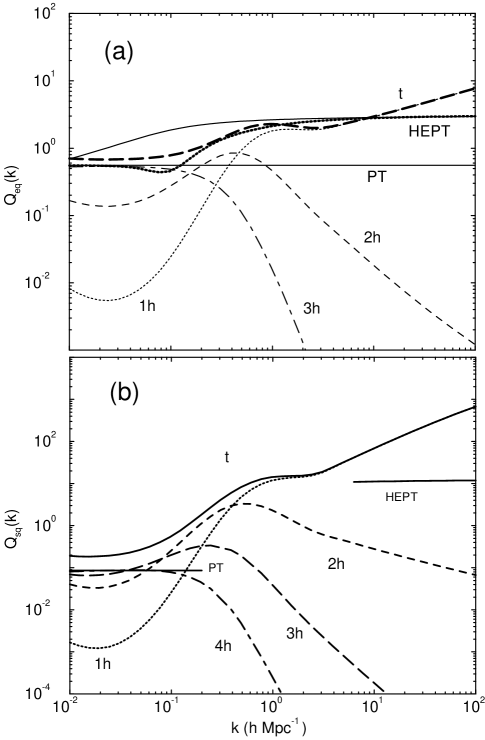
Figure 14 (from [236]) compares the predicted $Q_{\rm eq}$s with measurements in numerical simulations. To the resolution of the simulations, the data are consistent with perturbation theory at the largest scales, and with HEPT in the non-linear regime. The halo model predictions based on the two mass function choices (Press-Schechter and Sheth-Tormen) generally bracket the numerical simulation results, assuming the same halo profile and concentration–mass relations are the same in both cases. The most massive halos are responsible for a significant fraction of the total non-Gaussianity in the non-linear density field. This is shown in the bottom panel of Figure 14; when halos more massive than 10${}^{14}\,M_{\odot}/h$ are absent, $Q_{\rm eq}$ is reduced substantially (compare dashed and solid curves).

Figure 14: $Q_{\rm eq}(k)$ as a function of scale, (a) measured in numerical simulations and (b) compared to halo model predictions. In (a), the triangles are measurements in a box of size 100$h^{-1}$ Mpc while squares denote measurements in box sizes of 300$h^{-1}$ Mpc. The linear perturbation theory (PT) and hyperextended perturbation theory (HEPT) values are show as solid lines. In (b), the halo model predictions associated with Press-Schechter and Sheth-Tormen mass functions generally bracket the measurements. The dashed lines show the result of only including contributions from halos less massive than $10^{14}\,h^{-1}M_{\odot}$. They lie significantly below the solid curves, illustrating that massive halos provide the dominant contributions to these statistics. The figure is taken from [236].

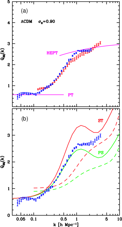
The halo based calculation suggests $Q_{\rm eq}$ increases, whereas HEPT suggests that $Q_{\rm eq}$ should remain approximately constant, on the smallest scales. These small scales are just beyond the reach of numerical simulations to date. As we discuss later, the scales where the two predictions differ significantly are not easily probed with observations either, at least at the present time.

For the trispectrum, and especially the contribution of trispectrum to the power spectrum covariance as we will soon discuss, we are mainly interested in terms of the form $T({\bf k}_{1},-{\bf k}_{1},{\bf k}_{2},-{\bf k}_{2})$, i.e. parallelograms which are defined by either the length $k_{12}$ or by the angle between ${\bf k}_{1}$ and ${\bf k}_{2}$. To illustrate, our results, we will take $k_{1}=k_{2}$ and the angle to be $90^{\circ}$ (${\bf k}_{2}={\bf k}_{\perp}$) so that the parallelogram is a square. It is then convenient to define

$$\Delta^{2}_{\rm sq}(k)\equiv\frac{k^{3}}{2\pi^{2}}T^{1/3}({\bf k},-{\bf k},{\bf k}_{\perp},-{\bf k}_{\perp})\,.$$ (120)

This quantity scales roughly as $\Delta^{2}(k)$. This spectrum is shown in figure 12(b) with the individual contributions from the 1h, 2h, 3h, 4h terms shown explicitly. At $k\mathchar 13350\relax 10k_{\rm nonlin}\sim 10h$Mpc^-1, $Q_{\rm sq}$ is due mainly from the single halo term.

As for $Q_{\rm eq}$, the halo model predicts that $Q_{\rm sq}$ will increase at high $k$. Numerical simulations do not quite have enough resolution to test this [236].

Figures 13(a) and (b) show that as one considers higher order statistics, the halo model predicts a substantial excess in power at linear scales compared to the perturbation theory value. This is another manifestation of the problem, noted in § 4.4, that, in positive perturbation models, the single-halo contribution to the power does not vanish as $k\to 0$. While this discrepancy appears large in the $Q_{\rm sq}$ statistic, it does not affect the calculations related to the covariance of large scale structure power spectrum measurements since, on linear scales, the Gaussian contribution usually dominates the non-Gaussian contribution. However, we caution that dividing the halo model calculation on linear scales by the linear power spectrum to obtain, say halo bias or galaxy bias, may lead to errors.

5.3 Power Spectrum Covariance

Table 2:

Dark Matter Power Spectrum Correlations
$k$ 0.031 0.058 0.093 0.110 0.138 0.169 0.206 0.254 0.313 0.385 0.031 1.000 0.041 0.086 0.113 0.149 0.172 0.186 0.186 0.172 0.155 0.058 (0.023) 1.000 0.118 0.183 0.255 0.302 0.334 0.341 0.328 0.305 0.093 (0.042) (0.027) 1.000 0.160 0.295 0.404 0.466 0.485 0.475 0.453 0.110 (0.154) (0.086) (0.028) 1.000 0.277 0.433 0.541 0.576 0.570 0.549 0.138 (0.176) (0.149) (0.085) (0.205) 1.000 0.434 0.580 0.693 0.698 0.680 0.169 (0.188) (0.138) (0.177) (0.251) (0.281) 1.000 0.592 0.737 0.778 0.766 0.206 (0.224) (0.177) (0.193) (0.314) (0.396) (0.484) 1.000 0.748 0.839 0.848 0.254 (0.264) (0.206) (0.261) (0.355) (0.488) (0.606) (0.654) 1.000 0.858 0.896 0.313 (0.265) (0.202) (0.259) (0.397) (0.506) (0.618) (0.720) (0.816) 1.000 0.914 0.385 (0.270) (0.205) (0.262) (0.374) (0.508) (0.633) (0.733) (0.835) (0.902) 1.000 $\sqrt{\frac{C_{ii}}{C_{ii}^{G}}}$ 1.00 1.02 1.04 1.07 1.14 1.23 1.38 1.61 1.90 2.26

NOTES.—Diagonal normalized covariance matrix of the binned dark matter density field power spectrum with $k$ in units of $h$ Mpc^-1. Upper triangle displays the covariance found under the halo model. Lower triangle (parenthetical numbers) displays the covariance found in numerical simulations by [185]. Final line shows the fractional increase in the errors (root diagonal covariance) due to non-Gaussianity as calculated using the halo model.

The trispectrum is related to the variance of the estimator of the binned power spectrum [235, 185, 76, 56]:

$$\hat{P}_{i}={1\over V}\int_{{\rm s}i}{d^{3}k\over V_{{\rm s}i}}\delta^{*}(-{\bf k})\delta({\bf k})\,,$$ (121)

where the integral is over a shell in $k$-space centered around $k_{i}$, $V_{{\rm s}i}\approx 4\pi k_{i}^{2}\delta k$ is the volume of the shell and $V$ is the volume of the survey. Recalling that $\delta({\bf 0})\rightarrow V/(2\pi)^{3}$ for a finite volume,

$$C_{ij}\equiv\left<\hat{P}_{i}\hat{P}_{j}\right>-\left<\hat{P}_{i}\right>\left<\hat{P}_{j}\right>={1\over V}\left[{(2\pi)^{3}\over V_{{\rm s}i}}2P_{i}^{2}\delta_{ij}+T_{ij}\right]\,,$$ (122)

where

$$T_{ij}\equiv\int_{{\rm s}i}{d^{3}k_{i}\over V_{{\rm s}i}}\int_{{\rm s}j}{d^{3}k_{j}\over V_{{\rm s}j}}T({\bf k}_{i},-{\bf k}_{i},{\bf k}_{j},-{\bf k}_{j})\,.$$ (123)

Although both terms scale in the same way with the volume of the survey, only the (first) Gaussian piece necessarily decreases with the volume of the shell. For the Gaussian piece, the sampling error reduces to a simple root-N mode counting of independent modes in a shell. The trispectrum quantifies the non-independence of the modes both within a shell and between shells. Therefore, calculating the covariance matrix of the power spectrum estimates reduces to averaging the elements of the trispectrum across configurations in the shell. For this reason, we now turn to the halo model description of the trispectrum.

To test the accuracy of the halo trispectrum, we compare dark matter correlations predicted by our method to those from numerical simulations by [185] (see also, [235]). Specifically, we calculate the covariance matrix $C_{ij}$ from equation (123) with the bins centered at $k_{i}$ and volume $V_{{\rm s}i}=4\pi k_{i}^{2}\delta{k_{i}}$ corresponding to their scheme. We also employ the parameters of their $\Lambda$CDM cosmology and assume that the parameters that defined the halo concentration properties from our fiducial $\Lambda$CDM model holds for this cosmological model also. The physical differences between the two cosmological model are minor, though normalization differences can lead to large changes in the correlation coefficients.

Figure 15: The correlations in dark matter power spectrum between bands centered at $k$ (see Table 1) and those centered at $k=0.031$h Mpc^-1 a (lower triangles) and $k=0.169$h Mpc^-1 ((upper squares). The open and filled symbols in these cases are for 200 h^-1 Mpc box simulations with 128³ and 256³ particles, respectively. The solid lines with filled circles represent the halo model predictions for same bands and are consistent with numerical simulations at the level of 10% or better. The figure is reproduced from [185].

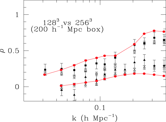
Table 2 compares the halo model predictions for the correlation coefficients

$$\hat{C}_{ij}={C_{ij}\over\sqrt{C_{ii}C_{jj}}}$$ (124)

with those measured in the simulations. Agreement in the off–diagonal elements is typically better than $\pm 0.1$, even in the region where non-Gaussian effects dominate, and the qualitative features such as the increase in correlations across the non-linear scale are reproduced. The correlation coefficients for two bands in the linear ($0.031h$ Mpc^-1) and non-linear ($0.169h$ Mpc^-1) regimes are shown in Figure 15. Triangles and squares show the values measured in the simulations, and filled circles and solid lines show the halo model predictions. The halo model is in agreement with numerical measurements over a wide range of scales, suggesting that it provides a reasonable way of estimating the covariance matrix associated with the dark matter power spectrum. In contrast, perturbation theory can only be used to describe the covariance and correlations in the linear regime while in the non-linear regime, and although the HEPT provides a reasonable description when $k_{i}\sim k_{j}$, it results in large discrepancies when $k_{i}\gg k_{j}$ [185, 235, 104].

Figure 16: Real-space moments with $p=3$ (skewness), 4 (kurtosis) and 5 as a function of smoothing scale. Squares and triangles show measurements in high and low resolution simulations, illustrating how difficult it is to make the measurement. Solid lines show the predictions based on the NFW profile but with Press-Schechter (lower) and Sheth-Tormen (upper) mass functions. Dashed line shows the HEPT prediction. The figure is from [236].

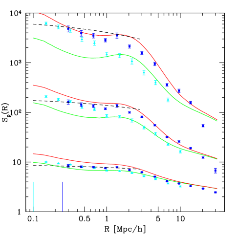
A further test of the accuracy of the halo approach is to consider higher order real-space moments such as the skewness and kurtosis. Figure 16 compares measurements of higher order moments in numerical simulations with halo model predictions: the halo model is in good agreement with the simulations.

5.4 Can we trust the halo model?

Figure 17: Ratio of the single halo term contribution to the total power when the distribution of concentrations at fixed mass is lognormal with width $\sigma_{{\rm ln}c}$, to that when $\sigma_{\ln c}\rightarrow 0$ for the power spectrum (a) and trispectrum (b). The small scale behavior, particularly of the higher order statistics, is sensitive to the high concentration tails of the $p(c|m)$ distribution.

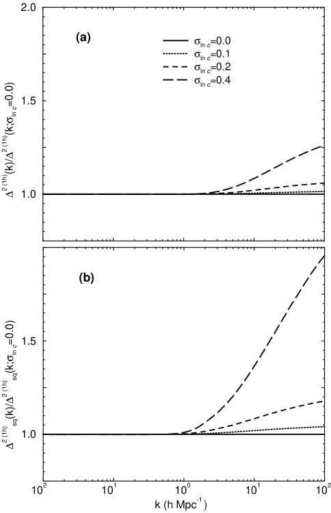
The halo model provides a physically motivated means of estimating the two-point and higher order statistics of the dark matter density field. However, it has several limitations which should not be forgotten when interpreting results. As currently formulated, the approach assumes all halos share a parameterized smooth spherically-symmetric profile which depends only on halo mass. However, we know that halos of the same mass have a distribution of concentration parameters, so that there is some variation in halo profile shape, even at fixed mass. In addition, halos in simulations are rarely smooth, and they are often not spherically symmetric.

It is straightforward to incorporate the distribution of halo concentrations into the formalism [56, 237]. In essence, a distribution $p(c|m)$ leads to changes in power at non-linear scales $k\mathchar 13350\relax 1h$ Mpc^-1. This is shown in Figure  17(a): the power on large linear scales is unaffected by a distribution $p(c|m)$, but the large $k$ power increases as the width of $p(c|m)$ increases. Increasing $\sigma_{\ln\,c}$ increases the power at small scales, because of the increased probabilty of occurence of high concentrations from the tail of the distribution. (Recall that simulations suggest $\sigma_{\ln\,c}\approx 0.25$.) Higher order statistics depend even more strongly on $\sigma_{\ln\,c}$, because they weight the large $c$ tails heavily. To illustrate, Figure 17(b) shows how the trispectrum, with ${\bf k}_{1}={\bf k}_{2}={\bf k}_{3}={\bf k}_{4}$, changes as $\sigma_{\ln\,c}$ increases.

Figure 18: Dark matter power spectrum (top) and reduced bispectrum for equilateral configurations (bottom) in numerical simulations (solid lines). Dashed lines show result of replacing halos with smooth M99 profiles and remaking the measurements. The replacement agrees with the original measurements up to the resolution limit of the simulation: $k\sim 10h$ Mpc^-1. Dotted curves are the linear and nonlinear expectation, based on fitting functions, in the case of the power spectrum and the linear perturbation theory result of $4/7$ in the case of $Q_{\rm eq}$. The figure is from [172].

Substructure is expected to contribute about 15% of the total dark matter mass of a halo (e.g., [280, 92]), and it will affect the power spectrum and higher order correlations on small scales. Measurements of $P(k)$ and $B(k)$ for equilateral triangles in which the actual clumpy nonspherical halo profiles in numerical simulations were replaced by smooth NFW or M99 halo profiles suggest that for $k\leq 10k_{\rm nonlin}$ or so, substructure and asphericities are not important (see Figure 18). A detailed discussion of how to account for this substructure is in [251].

No models to date account for departures from spherical symmetry, but this is mainly because until recently [139], there was no convenient parametrization of profile shapes which were not spherically symmetric. There is no conceptual reason which prevents one from including ellipsoidal halos in the model. Until this is done, note that spherically averaged profiles are adequate for modelling the power spectrum and other statistics which average over configurations, such as the $S_{n}$ parameters. The bispectrum is the lowest order statistic which is sensitive to the detailed shape of the halos. The dependence of bispectrum configuration on the spherical assumption was shown in some detail by [236]; they found that the spherical assumption may be the cause of discrepancies at the $\sim 20-30\%$ level between the halo model predictions and configuration dependence of the bispectrum in the mildly non-linear regime measured in simulations. Uncertainties in the theoretical mass function also produce variations at the 20% to 30% level (see, [135]).

Improvements to the halo model that one should consider include:
(1) Introduction of the asphericity of dark matter halos through a randomly inclined distribution of prolate and oblated ellipsoids. Recent work has shown that simply modifying the spherically symmetric profile shape to have different scale lengths along the three principal axes provides a reasonable parametrization of the ellipsoidal profiles of halos in numerical simulations, with the distribution of axis ratios depending on halo mass [139]. This makes it relatively straightforward to include asphericity in the model. Since the same ellipsoidal collapse model [257] which predicts the correct shape for the halo mass function (equation 59), can also be used to predict the distribution of halo axis ratios, it would be interesting to see if this distribution matches that in simulations. At the present time, shape information from X-ray observations of galaxy clusters is limited [49], although [Jeteatl02] argue that departures from spherical symmetry are necessary to correctly interpret their data.
(2) Incorporation of the effects of halo substructure. See [251] for a first step in this direction, which incorporates simple models of what is seen in numerical simulations [92, 28].
(3) Solution of the integral constraint problem at large scales discussed in § 4.4.

Figure 19: The angular two-point correlation function of galaxies in the SDSS early release data, for a number of bins in apparent $r^{*}$ band magnitude. In all cases, the correlation function is quite well described by a power law: $w(\theta)\propto\theta^{-0.7}$. The figure is from [46].

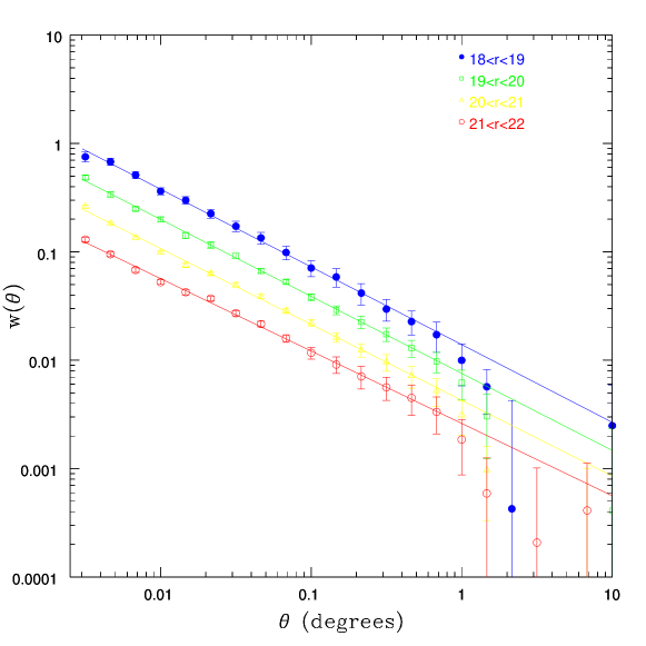
6 From Dark Matter to Galaxies

Figure 20: The PSC$z$ galaxy power spectrum (symbols, from [105]) compared to the dark matter power spectrum in a $\Lambda$CDM model (solid curve). We have fixed the amplitude of the dark matter power spectrum so that it matches the data on large scales. The discrepancy on smaller nonlinear scales suggests that the bias between the galaxies and the dark matter must be scale dependent.

Figure 21: Projected two-point correlation function of galaxies with absolute magnitude and redshift ranges indicated (left) and for different bins in color (right). In panel on left, squares, circles and triangles show results for faint, intermediate and luminous galaxies respectively. Although the more luminous galaxies are more strongly clustered, the same power-law slope provides a reasonable fit at all luminosities. In constrast, the slope of the power-law is a strong function of color. Both panels are from [298].

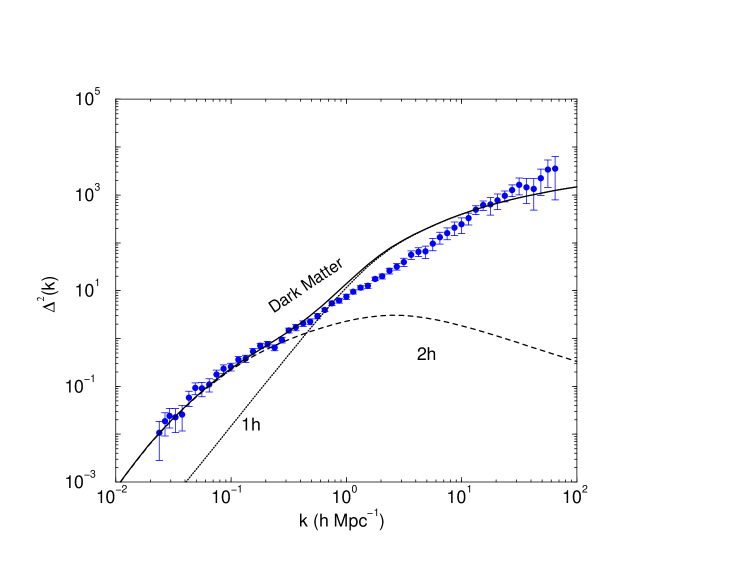
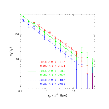
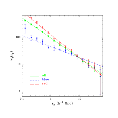
We have known since the late 1960’s that the angular correlation function of optically selected galaxies is a power law: $w(\theta)\propto\theta^{-(\gamma-1)}$, with $\gamma\approx 1.8$ [279]. Figure 19 shows a recent measurement of $w(\theta)$ from the SDSS collaboration [46]: it is also well described by this power law. This suggests that the three-dimensional correlation functions and power-spectra should also be power laws. The symbols in Figure 28 show that the power-spectrum of galaxies in the PSC$z$ survey as measured by [105] is accurately described by a power-law over a range of scales which spans about three orders of magnitude. More recently, the 2dFGRS [203] and SDSS [298] data show that, although more luminous galaxies cluster more strongly, for a wide range of luminosities, the three-dimensional correlation function is indeed close to a power law. Figure 21, from [298], shows that although the slope of the power-law is approximately independent of luminosity (left), it is a strong function of galaxy color; on small scales, redder galaxies have steeper correlation functions.

In contrast, a generic prediction of CDM models is that, at the present time, the two-point correlation function of the dark matter, and its Fourier transform, the dark matter power spectrum, are not power laws (see, e.g., the solid curve in Figure 28). Why is the clustering of galaxies so different from that of the dark matter?

6.1 The clustering of galaxies

In the approach outlined by White & Rees [292], baryonic gas can only cool and form stars if it is in potential wells such as those formed by virialized dark matter halos. As a result, all galaxies are expected to be embedded in dark halos (see figure 2). More massive halos may contain many galaxies, in which case it is natural to associate the positions of galaxies with subclumps within the massive halo; some, typically low mass, halos may contain no galaxies; but there are no galaxies which are without halos. Within this framework, the properties of the galaxy population are determined by how the gas cooling rate, the star formation rate, and the effects of stellar evolution on the reservoir of cooled gas, depend on the mass and angular momentum of the parent halo. There are now a number of different prescriptions for modeling these ‘gastrophysical’ effects [293, 157, 42].

Within the context of the halo model, the gastrophysics determines how many galaxies form within a halo, and how these galaxies are distributed around the halo center. Thus, the halo model provides a simple framework for thinking about and modeling why galaxies cluster differently than dark matter [137, 244, 212, 236, 253, 240, 11].

Suppose we assume that the number of dark matter particles in a halo follows a Poisson distribution, with mean proportional to the halo mass such that $\langle N_{dm}|m\rangle\propto m$, and $\langle N_{dm}(N_{dm}-1)|m\rangle\propto m^{2}$. Note that these proportionalities are the origin of the weighting by $m$ and $m^{2}$ in equation (LABEL:pkm) for $P^{2h}_{dm}(k)$ and $P^{1h}_{dm}(k)$. To model the power spectrum of galaxies, we, therefore, simply modify equation (LABEL:pkm) to read

$$P_{\rm gal}(k) = P^{1h}_{{\rm gal}}(k)+P^{2h}_{{\rm gal}}(k)\,,\qquad\qquad{\rm where}$$

$$P^{1h}_{{\rm gal}}(k) = \int dm\,n(m)\,\frac{\left<N_{\rm gal}(N_{\rm gal}-1)|m\right>}{\bar{n}_{\rm gal}^{2}}\,|u_{\rm gal}(k|m)|^{p}\,,$$

$$P^{2h}_{{\rm gal}}(k) \approx P^{\rm lin}(k)\left[\int dm\,n(m)\,b_{1}(m)\,\frac{\left<N_{\rm gal}|m\right>}{\bar{n}_{\rm gal}}\,u_{\rm gal}(k|m)\right]^{2}.$$ (125)

Here,

$$\bar{n}_{\rm gal}=\int dm\,n(m)\,\left<N_{\rm gal}|m\right>$$ (126)

denotes the mean number density of galaxies. On large scales where the two-halo term dominates and $u_{\rm gal}(k|m)\to 1$, the galaxy power spectrum simplifies to

$$P_{{\rm gal}}(k)\approx b_{\rm gal}^{2}\,P^{\rm lin}(k),$$ (127)

where

$$b_{\rm gal}=\int dm\,n(m)\,b_{1}(m)\,\frac{\left<N_{\rm gal}|m\right>}{\bar{n}_{\rm gal}}$$ (128)

denotes the mean bias factor of the galaxy population.

In addition to replacing the weighting by mass (i.e., the number of dark matter particles) with a weighting by number of galaxies, there are two changes with respect to equation (LABEL:pkm). First, $u_{\rm gal}(k|m)$ denotes the Fourier transform of the density run of galaxies rather than dark matter around the halo center. Although a natural choice is to approximate this integral by using the subclump distribution within a halo, we will show shortly that setting it to be the same as that of the dark matter (equation 79) is a reasonable approximation [258]. Second, in the single-halo term, the simplest model is to set $p=2$ for $P^{1h}_{dm}(k)$. However, in halos which contain only a single galaxy, it is natural to assume that the galaxy sits at the center of its halo. To model this, one would set $p=2$ when $\left<N_{\rm gal}(N_{\rm gal}-1)\right>$ is greater than unity and $p=1$ otherwise.

It is worth considering a little more carefully where these scalings in the one-halo term come from. Suppose that in a halo which contains $N_{\rm gal}$ galaxies, one galaxy sits at the halo centre. Each of the galaxies contributes a factor of $u_{\rm gal}$ to the power, except for the central galaxy which contributes a factor of unity. Pairs which come from the same halo are of two types: those which include the central galaxy, and those which do not. Since only the galaxies which are not at the centre get factors of $u_{\rm gal}$, the weighting must be proportional to

$$\sum_{N_{\rm gal}>1}p(N_{\rm gal}|m)\,\left[(N_{\rm gal}-1)\,u_{\rm gal}(k|m)+{(N_{\rm gal}-1)((N_{\rm gal}-2)\over 2}\,u_{\rm gal}(k|m)^{2}\right];$$

where $p(N_{\rm gal}|m)$ is the probability an $m-$halo contains $N_{\rm gal}$ galaxies, and the sum is from $N_{\rm gal}>1$ because, to contribute pairs, there must be at least two galaxies in the halo. The first term is the contribution from pairs which include the central galaxy, and the second term is the contribution from the other pairs. The sums over $N_{\rm gal}$ yield

$$\Bigl{[}\langle N_{\rm gal}-1|m\rangle+p(0|m)\Bigr{]}\,\Bigl{[}u_{\rm gal}(k|m)-u_{\rm gal}(k|m)^{2}\Bigr{]}$$

$$+\langle N_{\rm gal}(N_{\rm gal}-1)/2|m\rangle\,u_{\rm gal}(k|m)^{2}.$$

Evidently, to compute this term requires knowledge of $p(0|m)$. However, if we are in the limit where most halos contain no galaxies, then the leading order contribution to the sum above is $p(2|m)\,u_{\rm gal}(k|m)$. But, in this limit, $\langle N_{\rm gal}(N_{\rm gal}-1)|m\rangle\equiv\sum N_{\rm gal}(N_{\rm gal}-1)\,p(N_{\rm gal}|m)\approx 2\,p(2|m)$, so this leading order term should be well approximated by $\langle N_{\rm gal}(N_{\rm gal}-1)/2|m\rangle\,u_{\rm gal}(k|m)$. In the opposite limit of a large number of galaxies per halo, it should be accurate to set $p(0|m)\ll 1$. Then the expression above reduces to $\langle N_{\rm gal}-1|m\rangle\,[u_{\rm gal}(k|m)-u_{\rm gal}(k|m)^{2}]+\langle N_{\rm gal}(N_{\rm gal}-1)/2\rangle\,u_{\rm gal}(k|m)^{2}$. For Poisson counts, $\langle n(n-1)\rangle=\langle n\rangle^{2}$. If this is indicative of other count models also, then this shows that the dominant term is the one which comes from the second factorial moment. Therefore, it should be reasonable to approximate the exact expression above by $\langle N_{\rm gal}(N_{\rm gal}-1)|m\rangle\,u_{\rm gal}(k|m)$ when $\langle N_{\rm gal}(N_{\rm gal}-1)|m\rangle\leq 1$, and by $\langle N_{\rm gal}(N_{\rm gal}-1)|m\rangle\,u_{\rm gal}(k|m)^{2}$ otherwise. Notice that the two limits differ only by one factor of $u_{\rm gal}$.

The expressions above show explicitly that if $\langle N_{\rm gal}|m\rangle$ and $\langle N_{\rm gal}(N_{\rm gal}-1)|m\rangle$ are not proportional to $m$ and $m^{2}$ respectively, then the clustering of galaxies will be different from that of the dark matter, even if $u_{\rm gal}(k|m)=u_{dm}(k|m)$. Because the one- and two-halo terms are modified (with respect to the dark matter case) by two different functions, it may be possible to adjust them separately in such a way that they sum to give the observed power law.

Thus, the halo model shows that the distribution $p(N_{\rm gal}|m)$ determines whether or not $P_{\rm gal}(k)$ is a power law. Although the analysis above assumed that $p(N_{\rm gal}|m)$ depends only on $m$, it is very likely that other properties of a halo, than simply its mass, determine the number of galaxies in it. For example, $N_{\rm gal}$ almost certainly depends on the halo’s formation history. Since the concentration $c$ of the halo density profile also depends on the formation history [198, 78, 288], a convenient way to incorporate the effects of the formation history is to set $p(N_{\rm gal}|m,c)$, and then integrate over the lognormal scatter in halo concentrations when computing the halo model predictions. In what follows, we will ignore this subtlety.

Figure 22: The total luminosity in galaxies brighter than $M_{r^{*}}<-18$ which are in a halo, as a function of the total mass of the halo, from the semi-analytic galaxy formation models of [157]. Dashed lines show lines of constant mass-to-light ratio: the value of $M/L_{18}$ at $z=0.5$ shown is a factor of two smaller than at $z=0$.

Although the exact shape of $p(N_{\rm gal}|m)$ is determined by gastrophysics, there are some generic properties of it which are worth describing. Since galaxies form from baryons, a simple first approximation would be to assume that the first moment, $\langle N_{\rm gal}|m\rangle$, should be proportional to the mass in baryons, which, in turn, is likely to be a fixed fraction of the mass in dark matter of the parent halo. If we assume that $\langle N_{\rm gal}|m\rangle\propto m^{\alpha}$ (so $\mu=1$ is the scaling of the dark matter), then there are two reasons why we might expect $\alpha\leq 1$. Firstly, for the very massive halos, it is natural to associate galaxies with subclumps within the halo. The total number of subclumps within a massive parent halo which are more massive than a typical galaxy scales as $\alpha\approx 0.9$ [92]. Halo substructure as a plausible model for the galaxy distribution is discussed by [41, 158]. If one identifies all subclumps in CDM haloes which had velocity dispersions larger than about 100 km/s (which is typical for a small galaxy sized halo), then the correlation function of these objects is a power law of about the same slope and amplitude as that of optically selected galaxies. Remarkably, the slope and amplitude of this power law are approximately the same whether one identifies the subclumps at redshifts as high as $3$ or as low as $0$ (see [3] for a clear discussion of why this happens, and Figure 24 below).

Secondly, galaxy formation depends on the ability of baryons to cool. Since the velocity dispersion within a halo increases with halo mass, the efficiency of cooling decreases. This might lead to a reduction in the efficiency of galaxy formation at the high mass end relative to the low mass end. Such a mass dependent efficiency for galaxy formation has been used to explain the observed excess of entropy in galaxy clusters relative to smaller groups [25]. At the low mass end, one might imagine that there is a minimum dark halo mass within which galaxies can be found. This is because the energy feedback from supernovae which explode following an initial burst of star formation may be sufficient to expel the baryons from the shallower potential wells of low mass halos. Also, during the epoch of reionization at $z<6$, photoionization may increase the gas temperature. The temperature of the reheated gas may exceed the virial temperature of low mass halos, thus suppressing star formation in them [156, 30, 10].

Figure 23: The average number of galaxies as a function of dark matter halo mass in the semi-analytic galaxy formation models of [157]. Curves show the fits in equation (129).

Detailed semi-analytic galaxy formation models allow one to quantify these effects [157, 9]. The symbols in Figure 23 show how $\langle N_{\rm gal}|m\rangle$ depends on galaxy type and luminosity in the models of [157]. The lines show simple fits (from [253]):

$$\langle N_{\rm Blue}|m\rangle = 0.7\qquad\qquad{\rm if}\ 10^{11}\,M_{\hbox{$\odot$}}h^{-1}\leq m\leq M_{\rm Blue}$$

$$= 0.7\,(m/M_{\rm Blue})^{\alpha_{B}}\qquad{\rm if}\ m>M_{\rm Blue}$$

$$\langle N_{\rm Red}|m\rangle = (m/M_{\rm Red})^{\alpha_{R}}\qquad m\geq 10^{11}\,M_{\hbox{$\odot$}}h^{-1}$$

$$\langle N_{\rm gal}|m\rangle = \langle N_{\rm Blue}|m\rangle+\langle N_{\rm Red}|m\rangle,$$ (129)

where $M_{\rm Blue}=4\times 10^{12}\,M_{\odot}/h$, $\alpha_{\rm B}=0.8$, $M_{\rm Red}=2.5\times 10^{12}\,M_{\odot}/h$, and $\alpha_{\rm R}=0.9$.

Figure 24: The number of subclumps in a halo as a function of parent halo mass in a simulation at $z=1$ (left) and 3 (right). Top panel shows $\langle N\rangle$ (long dashed) and $\sqrt{\langle N(N-1)\rangle}$ (short dashed) as a function of mass for: all subclumps (upper lines) and for subclumps with mass greater than $10^{10}$ (middle) and $10^{11}h^{-1}M_{\odot}$ (lower), respectively. The lower solid line shows equation (129). Middle panel is similar, but with cuts on stellar mass: all subclumps (upper lines) and subclumps with stellar mass greater than $10^{9}$ (middle) and $10^{10}h^{-1}M_{\odot}$ (lower). Bottom panel shows cuts on star-formation rate: all subclumps (upper lines), and for subclumps with star formation rates greater than 1 (middle) and 10 (lower) $M_{\odot}$/yr.

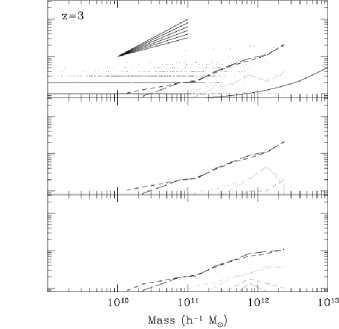
Figure 24 compares the distribution of subclumps in the numerical simulations of [291] with the expected number counts of galaxies within halos (equation (129). The number of semianalytic galaxies per halo scales similarly to the dark matter halo subclumps when the mass limit of subclumps are above $10^{11}h^{-1}$ M_⊙, suggesting that identifying halo subclumps with galaxies is a reasonable model.

Another interesting feature of these models in shown in Figure 25. The top and bottom panels show $\langle N_{\rm gal}|m\rangle$ and $\langle N_{\rm gal}(N_{\rm gal}-1)|m\rangle$ from the GIF models, but now we only show counts for galaxies which have absolute magnitudes in the range $-19\leq M_{r^{*}}\leq-20$. The top panels show that there is a pronounced peak in the number of galaxies per halo when $\langle N_{\rm gal}|m\rangle\leq 1$; in this regime, there is a relatively tight correlation between the luminosity of a galaxy and the mass of its parent halo. In the more massive halos which contain many galaxies, there is no correlation between luminosity and halo mass, and the number of galaxies scales approximately linearly with halo mass. Figure 23 is built up from a number of curves like those shown here.

Figure 25: The mean, $\langle N\rangle$, and second factorial moment, $\langle N(N-1)\rangle$ of the distribution of the number of galaxies per halo as a function of the halo mass $m$. Symbols show measurements in the semianalytic model of [157] and we have selected objects which are predicted to have absolute magnitudes between $-19$ and $-20$ in the SDSS $r^{*}-$band. Results for absolute magnitudes in the range $-17$ to $-18$, and $-18$ to $-19$ are qualitatively similar, although the peak for the lower luminosity bins shifts to lower masses.

The bottom panels in Figure 25 are also interesting. If $p(N_{\rm gal}|m)$ were Poisson, then $\langle N_{\rm gal}(N_{\rm gal}-1)|m\rangle=\langle N_{\rm gal}|m\rangle^{2}$. While the Poisson model is reasonably accurate at large $\langle N_{\rm gal}|m\rangle$, the scatter in $N_{\rm gal}$ at fixed $m$ can be substantially less than Poisson at the low mass end. This is largely a consequence of mass conservation [252]: the Poisson model allows an arbitrarily large number of galaxies to be formed from a limited amount of dark matter. For this reason, [236] argued that a binomial distribution should provide a convenient approximation to $p(N_{\rm gal}|m)$. A binomial is specified by its mean and its second moment. To match the semianalytic models, the mean must be given by equation (129), and the second moment by

$$\langle N_{\rm gal}(N_{\rm gal}-1)\rangle^{1/2}=\alpha(m)\,\langle N_{\rm gal}|m\rangle\,,$$ (130)

where $\alpha(m)=\log\sqrt{m/10^{11}h^{-1}M_{\hbox{$\odot$}}}$ for $m<10^{13}h^{-1}M_{\hbox{$\odot$}}$ and $\alpha(m)=1$ thereafter. The Binomial assumption allows one to model higher order correlations, since, by analogy with the two point correlation function, the halo model for $\xi_{n}$ depends on the $n-$th moment of $p(N_{\rm gal}|m)$. For example, the bi- and trispectra require knowledge of the third and fourth moments of $p(N_{\rm gal}|m)$.

Figure 26: Correlation functions of different tracers of the dark matter density field in the GIF $\Lambda$CDM semianalytic galaxy formation model. Filled circles are for the dark matter, crosses are for red galaxies,squares for galaxies which have low star formation rates, triangles for galaxies with high star formation rates, and open circles for blue galaxies. The two solid curves show the halo model predictions for the red and blue galaxies, and the dashed curves show what happens if we use the second factorial moment of the galaxy counts, rather than the second moment when making the model predicition. For comparison, the dotted curve shows the predicted dark matter correlation function. Bottom panel shows how the bias factor: $\sqrt{\xi(r)/\xi_{dm}(r)}$ depends on scale. The figure is from [260].

Figure 26 shows the result of inserting the $N_{\rm gal}-m$ relations shown in Figure 23 (equation (129) in the halo model, and changing nothing else (i.e., the red and blue galaxies are both assumed to follow the same NFW profile as the dark matter). The symbols show measurements in the GIF semianalytic models which equation (129) describes, and the curves, which provide a good fit, show the halo model prediction. On small scales, the redder galaxies have a steeper correlation function than the blue galaxies, in qualitative agreement with the SDSS measurements shown in Figure 21. The agreement between the simulations and the halo model calculation suggests that almost the entire difference between the clustering of red and blue galaxies is a consequence of the $N_{\rm gal}-m$ relation. The smaller additional effect which comes from allowing the red and blue galaxies to be distributed differently around the parent halo centre (e.g., if the reds are more centrally concentrated), is studied in some detail in [240].

The dependence of clustering on luminosity (Figure 21) is also straightforward to understand. If luminous galaxies reside in the more massive halos (this is a natural prediction of most semianalytic models), then, because the more massive halos are more strongly clustered (Figure 4), the more luminous galaxies should be more strongly clustered. The halo model also shows clearly that, in magnitude limited surveys such as the SDSS, this sort of luminosity dependent clustering must be taken into account when interpreting how the angular clustering strength depends on the magnitude limit, and when inverting $w(\theta)$ to estimate $P(k)$. If not, then the fact that the more strongly clustered luminous galaxies which are seen out to larger distances, and hence contribute to the largest scale power, will lead to erroneous conclusions about the true amount of large scale power.

Whereas most implementations of the halo model have concentrated on the $p(N_{\rm gal}|m)$ relation derived from semianalytic galaxy formation models (e.g., Figure 23), information about $p(N_{\rm gal}|m)$ is encoded in the luminosity functions of galaxies and clusters. For example, [212] argue that observations of the mass-to-light ratio in groups (e.g., plots like Figure 22, but made using data rather than semianalytic models), the combined luminosity function of galaxies in groups and clusters, and the galaxy luminosity function itself, can together be used to determine the mean number of galaxies per halo mass. The idea is to use the galaxy luminosity function to estimate a characteristic luminosity; use it to estimate the number of galaxies in a group by matching to the luminosity function of galaxies in groups and clusters; assign a mass to galaxy groups and clusters by requiring the observed number density of groups from the halo mass function agree with that obtained from the luminosity function. This leads to a measured mean number of galaxies of the form $\langle N_{\rm gal}|m\rangle\propto m^{0.92}$ which is close to that shown in, e.g., Figure 23. The SDSS galaxy cluster catalogs offer a promising opportunity to exploit this approach.

It is remarkable that this simple $N_{\rm gal}-m$ parametrization of the semianalytic models is all that is required to understand how and why the clustering depends on galaxy type. It is this fact which has revived interest in the halo model.

6.2 Galaxy–dark matter cross power spectrum

The halo model also suggests a simple parameterization of the cross-correlation between the galaxy and dark matter distributions [244, 99]:

$$P_{{\rm gal}-\rm dm}(k) = P^{1h}_{{\rm gal}-\rm dm}(k)+P^{2h}_{{\rm gal}-\rm dm}(k)\qquad\qquad{\rm where}$$

$$P^{1h}_{{\rm gal}-dm}(k) = \int dm\,{mn(m)\over\bar{\rho}}\,\frac{\left<N_{\rm gal}|m\right>}{\bar{n}_{\rm gal}}\,|u_{dm}(k|m)\,|\,|u_{\rm gal}(k|m)|^{p-1}\,$$

$$P^{2h}_{{\rm gal}-dm}(k) = P^{\rm lin}(k)\left[\int dm\,{mn(m)\over\bar{\rho}}\,b_{1}(m)u(k|m)\right]$$ (131)

$$\qquad\times\,\left[\int dm\,n(m)\,b_{1}(m)\frac{\left<N_{\rm gal}\right>}{\bar{n}_{\rm gal}}u_{\rm gal}(k|m)\right],$$

and, as before, one sets $p=1$ if $\left<N_{\rm gal}\right><1$ and one is interested in requiring that one galaxy always sits at the halo center. This expression is easily generalized to the cross-correlation between two galaxy samples.

If one galaxy always sits at the halo centre, then these expressions must be modified. To see the effect of this on the two-halo term, we must average both pieces of the two halo term over $p(n|m)$, with the requirement that $n>0$. This requires evaluation of sums of the form

$$\sum_{n>0}[1+(n-1)u(k|m)]\,p(n|m)=1-p(0|m)+\langle n-1|m\rangle\,u(k|m)+u(k|m)\,p(0|m)$$

which we could also have written as

$$N_{\rm eff}(k|m)\equiv[1-p(0|m)]\,[1-u_{\rm gal}(k|m)]+\langle n|m\rangle\,u_{\rm gal}(k|m).$$

Since both factors in the first term are positive, this shows clearly that there is an enhancement in power which comes from always placing one galaxy at the halo centre. Since $u(k|m)$ decreases as $k$ increases, the enhancement in power is largest on small scales (large $k$). In sufficiently massive halos one might expect to have many galaxies, and so $p(0|m)\ll 1$. In this limit, the expression above becomes $1-u(k|m)+\langle n|m\rangle\,u(k|m)=1+\langle n-1|m\rangle\,u(k|m)$. On the other hand, if most halos have no galaxies, then $p(1|m)$ is probably much larger than all other $p(n|m)$ with $n\geq 2$. Then the leading order term in the sum above is $p(1|m)$. Since $\langle n|m\rangle\equiv\sum np(n|m)\approx p(1|m)$, we have that $N_{\rm eff}(k|m)\approx\langle n|m\rangle$. In this limit, only a fraction $\langle n|m\rangle\ll 1$ of the halos contain a galaxy, and the galaxy sits at the halo centre, so there is no factor of $u$.

The contribution of the galaxy counts to the one halo term of the galaxy–mass correlation function is similar. Using the expressions above yields

$$P_{\rm gm}^{\rm 1h}(k) = \int{\rm d}m\,n(m)\,{m\over\bar{\rho}}\,|u(k|m)|\,{N_{\rm eff}(k|m)\over\bar{n}_{\rm gal}}$$

$$P_{\rm gm}^{\rm 2h}(k) \approx P_{\rm lin}(k)\ \left[\int{\rm d}m\,n(m)\,{m\over\bar{\rho}}\,b(m)\,u(k|m)\right]\$$ (132)

$$\qquad\qquad\times\left[\int{\rm d}m\,n(m)\,b(m)\,{N_{\rm eff}(k|m)\over\bar{n}_{\rm gal}}\right].$$

If the run of galaxies around the halo centre is not the same as of the dark matter, then one simply uses $u_{\rm gal}$ instead of $u$ in $N_{\rm eff}$. If the two-halo term usually does not dominate the power on small scales (this is almost always a good approximation), it is reasonable to ignore the enhancement in power associated with the central galaxy, and to simply set $N_{\rm eff}(k|m)\approx\langle n|m\rangle\,u_{\rm gal}(k|m)\approx\langle n|m\rangle$. The one-halo term requires knowledge of $p(0|m)$. Since $p(0|m)$ is usually unknown, the approximation above interpolates between the two limits discussed earlier by setting $N_{\rm eff}=\langle n|m\rangle\,u(k|m)$ if $\langle n|m\rangle\geq 1$, and $N_{\rm eff}=\langle n|m\rangle$ if $\langle n|m\rangle<1$.

In what follows, it will be convenient to define the cross-correlation coefficient:

$$r(k)\equiv\frac{P_{{\rm gal}-\rm dm}(k)}{\sqrt{P_{dm}(k)\,P_{{\rm gal}}(k)}}\,.$$ (133)

Note that $r(k)$ may depend on scale $k$.

Because we cannot measure the clustering of dark matter directly, the galaxy–dark matter cross-correlation is not observable. However, if one cross-correlates the galaxy distribution with weak lensing shear measurements, then the resulting signal is sensitive to this cross-correlation [244, 99]. We discuss this further in § 8.7.

6.3 Discussion

Figure 27: (a) Contributions by halo mass to the one-halo term in the halo model description of the power spectrum. (b) The same, but for the dark matter-galaxy cross-correlation power spectrum. At small scales, there is effectively no contribution from the smallest mass halos for the galaxy power spectrum. This figure is from [244].

Figure 28: The PSC$z$ galaxy power spectrum (symbols) and the result of tuning the first two moments of $p(N_{\rm gal}|m)$ so as to produce the power law like behavior (solid curve).

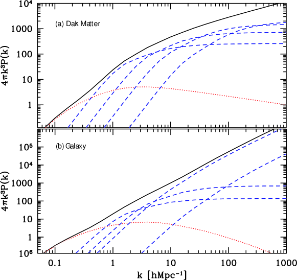
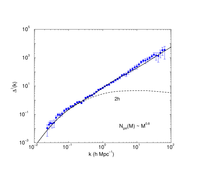
Figure 20 showed the galaxy power spectrum from the PCSZ survey [105]. The nonlinear dark matter power spectrum, scaled with a constant ($k-$independent bias factor) to match the linear regime cannot also match the power on small scales: this shows that the bias between dark matter and galaxies must depend on scale.

The top panel in Figure 27 shows the contributions to the dark matter power spectrum as a function of halo mass. The halo model description of the galaxy power spectrum shows clearly that the $p(N_{\rm gal}|m)$ distribution changes the relative contributions of low and high–mass halos to the total power, and so modifies the shape of the power spectrum in a way which depends on $k$.

The main change to the amplitude of the small-scale contribution to the galaxy power spectrum, the change which results in a power-law shape, comes from the halos which contain at least one galaxy, or, effectively halos containing what are called field or isolated galaxies. The assumption that these galaxies are at the center of the halo they occupy results in a power-law at small scales [212]. As discussed in [236], the contribution to the total power from such halos is very sensitive to the low-mass cutoff in the galaxy-mass relation. Thus, the small scale clustering of galaxies essentially allows one to constrain certain parameters related to the galaxy formation, such as the minimum mass in which a galaxy can exist.

Also, as shown in figure 27, at intermediate scales, the massive halos contribute less to the galaxy-dark matter power spectrum than to the dark matter power spectrum. This is because the $N_{\rm gal}\sim M^{0.8-0.9}$ weighting suppresses the contribution from the high mass end of dark matter halos. Figure 28 compares the associated galaxy power spectrum with that measured in the PCSZ survey. Note the power law behavior of the galaxy power spectrum over three to four decades in wavenumber.

In the halo model, galaxy power spectra and higher order correlations, when studied as a function of galaxy type or environment, allow one to extract certain galaxy properties such as the mean $N_{\rm gal}-m$ relation, and the mean mass of dark matter halos in which galaxies reside. This information may be helpful for understanding the galaxy formation and evolution processes. In [236] and [237], constraints on $p(N_{\rm gal}|m)$ were obtained by comparing halo model predictions with the measured variance and higher order correlations of galaxies in the APM [176] and PSCZ surveys. The halo based contraints of galaxy formation models are likely to increase with ongoing wide-field surveys such as the Sloan Digital Sky Survey (SDSS) and the 2dFGRS. The halo approach to galaxy clustering has already become helpful for interpreting the SDSS two-point galaxy correlation function [69] and the lensing-mass correlation [99].

7 Velocities

One of the great strengths of the halo-based approach is that it provides a clear prescription for identifying the scale on which perturbative approaches will break down, and non-linear effects dominate. The separation of linear and non-linear scales is an important tool when describing large scale velocities and related statistics. We now present the halo model description of velocities by extending [249, 253].

7.1 Velocities of and within halos

In the model, all dark matter particles are assumed to be in approximately spherical, virialized halos. The velocity of a dark matter particle is the sum of two terms,

$$v=v_{\rm vir}+v_{\rm halo}:$$ (134)

the first is due to the velocity of the particle about the center of mass of its parent halo, and the second is due to the motion of the center of mass of the parent. We will assume that each of these terms has a dispersion which depends on both halo mass and on the local environment, so that

$$\sigma^{2}(m,\delta)=\sigma^{2}_{\rm vir}(m,\delta)+\sigma^{2}_{\rm halo}(m,\delta).$$ (135)

The expression above assumes two things: the rms velocities depend on halo mass and local density only, and that the rms virial velocity within a halo is independent of the motion of the halo itself. Presumably both assumptions break down if the dark matter is collisional and/or dissipative. For collisionless matter, the assumption that the virial motions within a halo is independent of the halo’s environment is probably reasonably accurate. It is not clear that the same is true for halo speeds. Indeed, it has been shown that halos in dense regions move faster than those in underdense regions [42, 253]. It will turn out, however, that the fraction of regions in which $\sigma^{2}_{\rm halo}(m,\delta)$ is significantly different from $\sigma^{2}_{\rm halo}(m,0)$ is quite small. This means that neglecting the density dependence of halo velocities should be a reasonable approximation.

Consider the first term, $v_{\rm vir}$. We will assume that virialized halos are isothermal spheres, so that the distribution of velocities within them is Maxwellian. This is in reasonable agreement with measurements of virial velocities within halos in numerical simulations. If $\sigma_{vir}$ denotes the rms speeds of particles within a halo, then the virial theorem requires that

$${Gm\over r}\propto\sigma_{vir}^{2}\propto{H(z)^{2}\over 2}\,\Delta^{1/3}_{vir}(z)\left(3m\over 4\pi\rho_{crit}(z)\right)^{2/3}\,$$ (136)

where the final proportionality comes from the fact that all halos have the same density whatever their mass: $m/r^{3}\propto\Delta_{vir}\,\rho_{crit}$. This shows that $\sigma_{vir}\propto m^{1/3}$: the more massive halos are expected to be ‘hotter’. At fixed mass, the constant of proportionality depends on time and cosmology, and on the exact shape of the density profile of the halo. A convenient fitting formula is provided by [24]:

$$\sigma_{\rm vir}(m,z)=102.5\,g_{\sigma}\,\Delta^{1/6}_{\rm vir}(z)\,\left(H(z)\over H_{0}\right)^{1/3}\left({m\over 10^{13}M_{\odot}/h}\right)^{1/3}\ {{\rm km}\over{\rm s}},$$ (137)

where $g_{\sigma}=0.9$, and

$$\Delta_{\rm vir}=18\pi^{2}+60x-32x^{2},\qquad{\rm with}\quad x=\Omega(z)-1\,$$ (138)

and $\Omega(z)=[\Omega_{m}\,(1+z)^{3}]\,[H_{0}/H(z)]^{2}$. This fitting formula for the average density within a virialized object, $\Delta_{vir}\,\rho_{crit}$, generalizes the value $18\pi^{2}$ given previously for an Einstein de-Sitter universe in equation (52).

In [253], it was shown that this virial relation between mass and velocities is independent of the local environment. In practice, however, $\sigma_{vir}$ may depend on position within the halo. Accounting for the fact that halos really have more complicated density and velocity profiles is a detail which complicates the analysis, but not the logic of the argument. If the virialized halo is an isothermal sphere, the density run around the halo center falls as the square of the distance, then $\sigma_{vir}$ is the same everywhere within the halo. In practice, halos are not quite isothermal, but we will show later that the scaling above is still both accurate and useful.

We now turn to the second term, $v_{\rm halo}$. It will prove more convenient to first study halo speeds after averaging over all environments, before considering the speeds as a function of local density. This is similar to the order in which we discussed the halo mass function and its dependence on density. We first consider a halo of size $r$ at the present time. Because the initial density fluctuations were small, the particles in this halo must have been drained from a larger region $R$ in the initial conditions: $R/r\approx\Delta_{\rm vir}^{1/3}$, where $\Delta_{\rm vir}\approx 200$ or so. This means, for example, that massive halos were assembled from larger regions than less massive halos. Suppose we compute the rms value of the initial velocities of all the particles which make up a given halo and extend to include all halos of mass $m$, then we have effectively computed the rms velocity in linear theory, smoothed on the scale $R(m)\propto m^{1/3}$.

It is well known that the linear theory prediction for the evolution of velocities is more accurate than the linear theory prediction for the evolution of the density [216]. In what follows, we will assume that at the present time, the velocities of halos are reasonably well described by extrapolating the velocities of peaks and are smoothed on the relevant scale, $R\propto m^{1/3}$, using linear theory. For Gaussian initial conditions, this means that any given value of $v_{\rm halo}$ is drawn from a Maxwellian with dispersion $\sigma^{2}_{\rm halo}(m)$ given by:

$$\sigma_{\rm halo}(m)=H_{0}\Omega_{m}^{0.6}\ \sigma_{-1}\ \sqrt{1-\sigma_{0}^{4}/\sigma_{1}^{2}\sigma_{-1}^{2}},$$ (139)

where,

$$\sigma_{j}^{2}(m)={1\over 2\pi^{2}}\int{\rm d}k\ k^{2+2j}\,P^{\rm lin}(k)\,W^{2}[kR(m)],$$

and $W(x)$ is the Fourier transform of the smoothing window. The factor $H_{0}\Omega_{m}^{0.6}$ comes from a well-known approximation to the derivative of the growth function, with $d\log G/d\log a\sim\Omega_{m}^{0.6}$ when $a$ is the scale factor. Notice that the predicted rms velocity depends both on cosmology and on the shape of the power spectrum. The term under the square-root arises from the peak constraint [6]—it tends to unity as $m$ decreases: the peak constraint becomes irrelevant for the less massive, small $R$, objects.

Figure 29: Dependence on halo mass of the non-linear ($\sigma_{\rm vir}$) and linear theory ($\sigma_{\rm halo}$) terms in our model. Solid curves show the scaling we assume, and symbols show the corresponding quantities measured in the $z=0$ output time of the $\Lambda$CDM GIF simulation. Error bars show the 90 percentile ranges in mass and velocity. Dashed curve in panel on right shows the expected scaling after accounting for the finite size of the simulation box. Symbols and curves in the bottom of the panel on the right show the predicted and actual velocities at $z=20$.

In figure 29, we compare the dependence on mass for the two velocity terms in numerical simulations by the GIF collaboration [157] and the dependences we have discussed above. The symbols with error bars show the median and ninety percentile ranges in mass and velocity. Open squares, filled squares, open circles and filled circles show halos which have $60-100$, $100-10^{3}$, $10^{3}-10^{4}$ and $10^{4}-10^{5}$ particles, respectively. There are two sets of symbols in the panel on the right. For the time being, we are only interested in the symbols in the upper half which show halo velocities at $z=0$. The solid curves in the two panels show the scalings we assume.

Although the scaling of the virial term with mass is quite accurate, it appears that the extrapolated linear theory velocities are slightly in excess of the measurements in the simulations. This is almost entirely due to the finite size of the simulation box. The upper dashed curve shows the effect of using equation (139) to estimate the rms speeds of halos, after setting $P(k)=0$ for $k<2\pi/L$, where $L$ is the box-size: $L=141$ Mpc/$h$. Thus, the two panels show that our simple estimates of the two contributions to the variance of the velocity distribution are reasonably accurate.

Notice that the two terms scale differently with halo mass; indeed, to a first approximation, one might even argue that halo speeds are independent of halo mass. Figure 29 shows that $\sigma_{\rm halo}(m)<\sigma_{\rm vir}(m)$ for massive halos. Since massive halos have larger dispersions than less massive halos, the large velocity tail of $f(v)$ is determined primarily by the non-linear virial motions within massive halos, rather than by the peculiar motions of the halo centers of mass. For this reason, the large velocity tail of $f(v)$, at least, is unlikely to be sensitive to inaccuracies in our treatment of halo velocities, or to our neglect of the possibility that halo speeds may depend on the environment. Before moving on, note that our finding that massive halos are hotter, whereas the speeds with which halos move is approximately independent of mass, suggests that if massive halos occupy denser regions, then, we expect a temperature–density relation such that denser regions should be hotter. We will return to this later.

7.2 The distribution of non-linear velocities

In an ideal gas, the distribution of particle velocities $f(v)\,{\rm d}v$ has the Maxwell-Boltzmann form: each cartesian component of the velocity is drawn from an independent Gaussian distribution. Because of the action of gravity, the dark matter distribution at the present time is certainly not an ideal gas; numerical simulations show that $f(v)\,{\rm d}v$ is very different from a Maxwell–Boltzmann [231]; the distribution of each component of the velocity has an approximately Gaussian core with exponential wings. The halo model decomposition of peculiar velocities into linear and non-linear contributions (equation 134), provides a simple explanation for why this is so [249, 253].

Let $p(v|m)\,{\rm d}v$ denote the probability that a particle in a halo of mass $m$ has velocity in the range d$v$ about $v$. Then the total distribution is given by summing up the various $p(v|m)$ distributions, weighting by the fraction of particles which are in halos of mass $m$:

$$f(v)={\int{\rm d}m\,mn(m)\,p(v|m)\over\int{\rm d}m\,mn(m)}=\int{\rm d}m\,{mn(m)\over\bar{\rho}}\,p(v|m),$$ (140)

where $n(m)\,{\rm d}m$ is the number density of halos that have mass in the range d$m$ about $m$. The weighting by $m$ reflects the fact that the number of dark matter particles in a halo is supposed to be proportional to the halo mass. This expression holds both for the size of the velocity vector itself, which we will often call the speed, as well as for the individual velocity components.

To proceed, we need a model for the actual shape of $p(v|m)$. Since $v$ is the sum of two random variates (equation 134), we study each in turn. The virial motions are assumed to be Maxwellian. Also, for Gaussian initial density fluctuations, the linear peaks theory model of the halo motions means that they too are Maxwellian. Thus, in the model, each of the three cartesian components of the velocity of a dark matter particle in a clump of mass $m$ is given by the sum of two Gaussian distributed random variates, one with dispersion $\sigma^{2}_{\rm vir}(m)/3$ and the other with $\sigma^{2}_{\rm halo}(m)/3$. If we further assume that the motion around the clump center is independent of the motion of the clump as a whole, then these two Gaussian variates are independent and $p(v|m)$ is a Maxwellian with a dispersion which is the sum of the individual dispersions given by the sum in quadrature of equations (137) and (139).

In practice, we are only likely to observe velocities along the line of sight. Thus, we will eventually be interested in the distribution of $f(v)$ projected along the line of sight. Projection changes the Maxwellian $p(v|m)$ distributions into Gaussians:

$$p(v|m)={{\rm e}^{-[v/\sigma(m)]^{2}/2}\over\sqrt{2\pi\sigma^{2}(m)}}\qquad{\rm where}\ \sigma^{2}(m)={\sigma^{2}_{vir}(m)\over 3}+{\sigma_{halo}^{2}(m)\over 3};$$ (141)

i.e., $\sigma^{2}(m)$ is one third of the sum in quadrature of equations (137) and (139).

Now, $\sigma^{2}_{vir}(m)/\sigma^{2}_{v}(m*)=(m/m*)^{2/3}$, whereas $\sigma_{halo}^{2}$ is independent of halo mass (Figure 29). Therefore, the characteristic function of $f(v)$ is

$$\int dv\ {\rm e}^{ivt}f(v) = \int dm\ mn(m)\ \int dv\ {\rm e}^{ivt}p(v|m)$$ (142)

$$= \int dm\ mn(m)\ {\rm e}^{-t^{2}\sigma_{vir}^{2}(m)/6}\ {\rm e}^{-t^{2}\sigma_{halo}^{2}/6}$$

$$= {\rm e}^{-t^{2}\sigma_{halo}^{2}/6}\int{d\nu\over\nu}\sqrt{\nu\over 2\pi}\,{\rm e}^{-\nu/2}\ {\rm e}^{-t^{2}\sigma_{vir}^{2}(\nu)/6}$$

$$= {{\rm exp}(-t^{2}\sigma_{halo}^{2}/6)\over[1+t^{2}\sigma_{vir}^{2}(m*)/3]^{1/2}}.$$

The penultimate expression uses equation (57) for the halo mass function and assumes that the initial spectrum of fluctuations was scale free with $P(k)\propto k^{-1}$, which should be a reasonable approximation to the CDM spectrum on cluster scales. The final expression is quite simple: it is the product of the Fourier transforms of a Gaussian and a $K_{0}-$Bessel function. Therefore, $f(v)$ is the convolution of a Gaussian with a $K_{0}-$Bessel function. The Bessel function has exponential wings. Because the dispersion of the Gaussian and the Bessel function are similar, equation (142) shows that $f(v)$ should have a Gaussian core which comes from the linear theory halo motions, with exponential wings which come from the non-linear motions within halos.

Figure 30: The distribution of one-dimensional peculiar velocities for dark matter particles in a $\Lambda$CDM cosmology. Histograms show the distribution of the three cartesian components measured in GIF simulations. Dashed and dot-dashed curves show Gaussian and exponential distributions which have the same dispersion. The solid curve shows the distribution predicted by our model, after accounting for the finite size of the simulation box. The exponential wings are almost entirely due to virial motions within halos.

Figure 30 shows the one-dimensional $f(v)$ distribution given by inserting equations (141) and (59) in equation (140) for the same cosmological model presented in Figure 29. The histograms show the distribution measured in GIF simulations. For comparison, the dashed and dot-dashed curves in each panel show Gaussians and exponential distributions which have the same dispersion. The solid curves show the distribution predicted by the halo-based model: note the exponential wings, and the small $|v|$ core that is more Gaussian than exponential. The exponential wings are almost entirely due to non-linear motions within massive halos, so they are fairly insensitive to our assumptions about how fast these halos move.

It is worth emphasizing that $\sigma(m)$ in equation (141) is set by the cosmological model and the initial conditions. Thus, the second moment of the distribution in Figure 30 is not a free parameter. This halo model for $p(v|m)$ can be thought of as a simple way in which contributions to the velocity distribution statistic are split up into a part which is due to non-linear effects, given by the first term in equation 134, and a part which follows from extrapolating linear theory to a later time, denoted by the second term of that equation. The agreement with simulations suggests that this simple treatment of non-linear and linear contributions to the statistic are quite accurate.

Before moving on, note that the second moment of this distribution gives the mass-weighted velocity dispersion:

$$\sigma_{vel}^{2}=\int dm\frac{mn(m)}{\bar{\rho}}\left[\sigma^{2}_{vir}(m)+\sigma_{halo}^{2}(m)\right]\,.$$ (143)

This quantity is a measure of the total kinetic energy in the Universe, and hence is directly related to the Layzer-Irvine Cosmic Energy equation [258]. Observational estimates of this quantity are discussed by [65]. Because the virial velocities within massive halos are substantially larger the motions of the halos themselves (Figure 29), setting

$$\sigma_{halo}^{2}(m) \approx H^{2}f(\Omega_{m})^{2}\int\frac{dk}{2\pi^{2}}P(kr)|W(kR(m)|^{2}\,$$ (144)

(i.e., ignoring the peak constraint and simply assuming that halo velocities trace the linear velocity field smoothed at the scale from which halos collapsed) is a reasonable approximation. This expression for $\sigma_{vel}$ will be useful in the analyses of the CMB which follow.

7.3 Pairwise velocities

It is reasonable to expect that, as a result of their gravitational interaction, pairs of particles will, on average, approach each other. The gravitational attraction depends on separation, and it must fight the Hubble expansion which also depends on separation, so one might expect the mean velocity of approach to depend on the separation scale $r$. In fact, pair conservation provides a relation between the rate at which the correlation function on scale $r$ evolves, and the mean pairwise motion at that separation. In particular, pair conservation requires the mean peculiar velocity between a pair of particles at separation $r$ to satisfy [216]

$$-\frac{v_{12}(r)}{Hr}=\frac{1}{3[1+\xi(r)]}\frac{\partial(1+\bar{\xi})}{\partial\ln a}\,,$$ (145)

where $\bar{\xi}(x)$ is the volume averaged correlation function on proper scale $x$, $\bar{\xi}(x)=3x^{-3}\int_{0}^{x}dyy^{2}\xi(y)$. Since we have an accurate model for $\xi(r)$, we can use it to estimate $v_{12}(r)$. Before we do so, it is useful to see what linear theory would predict.

Figure 31: The ratio of mean streaming velocity of dark matter particles at scales separated by $r$, to the Hubble expansion at that scale. Triangles show the Virgo simulation measurements, circles show the GIF $\Lambda$CDM simulation, and dot-dashed curves show the Hubble expansion velocity. Crosses show the result of using the [210] formulae for the correlation function in the fitting formula provided by [142]. Solid curves show the halo model described here which accounts for the fact that the nonlinear evolution is different from what linear theory predicts, and then weights the linear and nonlinear scalings by the relative fractions of linear and nonlinear pairs. Dashed curves show the two contributions to the streaming motion in the halo model; the curves which peak at large $r$ are for pairs in two different halos. Dotted curve shows the approximation of using the linear theory correlation function to model this two-halo term.

In linear theory, $\partial\bar{\xi}/\partial\ln a\approx 2f(\Omega_{m})\bar{\xi}$, where $f(\Omega_{m})$ comes from the usual approximation to the derivative of the growth function: $f(\Omega_{m})\equiv\partial\ln G/\partial\ln a\approx\Omega_{m}^{0.6}$. Thus, in linear theory,

$$-\frac{v_{12}(r)}{Hr}=\frac{2f(\Omega_{m})\bar{\xi}(r,a)}{3[1+\xi(r,a)]}\,.$$ (146)

On large scales where linear theory analyses can still be applied, $\xi(r,a)\ll 1$. If we can drop this term from the denominator then this expression for the mean pairwise velocity is the same as that obtained directly from linear theory [102, 202, 142]. This linear theory expression underestimates velocities on small nonlinear scales by a factor of $\sim$ 3/2.

If we use the halo model decomposition $\xi=\xi_{1h}+\xi_{2h}$, and then use the fact that $\xi_{2h}$ scales like the linear theory correlation function, then equation (145) becomes

$$-\frac{v_{12}(r)}{Hr}=\frac{1}{3[1+\xi(r,a)]}\left[2f(\Omega_{m})\bar{\xi}_{2h}(r,a)+\frac{\partial\bar{\xi}_{1h}}{\partial\ln a}\right]\,.$$ (147)

The next step is to compute the derivative of the single halo term. Since $\xi_{1h}$ depends on the halo mass function and density profiles, the derivative can be computed directly [173, 258]:

$${\partial\bar{\xi}_{1h}\over\partial{\rm ln}a} = {\partial{\rm ln}m_{*}\over\partial{\rm ln}a}\Bigl{[}\bar{\xi}_{1h}(r,a)-\xi_{1h}(r,a)\Bigr{]}$$ (148)

$$\ \ +\ {3\over r^{3}}\int_{0}^{r}{\rm d}r^{\prime}\,{r^{\prime}}^{2}\int_{0}^{\infty}{\rm d}m{n(m)\over\bar{\rho}}{\lambda(r|m)\over\bar{\rho}}{\partial{\,\rm ln}\lambda\over\partial{\,\rm ln}a}\,,$$

where $\lambda(r|m)$ denotes the convolution of the density profile with itself:

$$\lambda(r|m)=2\pi\int dy\,y^{2}\,\rho(y|m)\int_{-1}^{1}d\beta\,\rho(z|m)|_{z^{2}=y^{2}+r^{2}-2yr\beta}\,.$$ (149)

Now, $\partial\ln\lambda/\partial\ln a\approx(\partial\ln\lambda/\partial\ln c)(\partial\ln c/\partial\ln a)_{m/m_{*}}$; since the time dependence of $c$ only comes from its dependence on $m_{*}$ and the derivative is taken by keeping $m_{*}$ constant, this term is zero. The piece which remains depends on $\partial\ln m_{*}/\partial\ln a$. If $P(k)\propto k^{n}$, then $\partial\ln m_{*}/\partial\ln a=f(\Omega_{m})6/(3+n)$ and [258]

$$-{v_{\rm 12}\over Hr} = {f(\Omega)\over 3[1+\xi(r,a)]}\Biggl{[}2\bar{\xi}_{2h}(r,a)+{6\over 3+n_{*}}\Bigl{[}\bar{\xi}_{1h}(r,a)-\xi_{1h}(r,a)\Bigr{]}\Biggr{]},$$ (150)

where $n_{*}=-1.53$ is the slope of the power spectrum on scale $m_{*}$ for the $\Lambda$CDM cosmology. Figure 31 compares the mean pairwise velocities from this halo model calculation with measurements in numerical simulations.

Extending the approach to estimate how the mean pairwise velocity of halos or of galaxies depends on scale requires modeling the halo or galaxy correlation function. This in turn requires estimating how the halo-mass dependent bias factors evolve. The evolution of the bias factors is straightforward to compute [260]. The resulting 2-halo contribution to $v_{12}$ is

$${v_{12}^{\rm 2i}(r)\over Hr}\approx{v_{12}^{\rm dm}(r)\over Hr}\ b_{i}\ \left[{1+\xi^{\rm lin}_{\rm dm}(r)\over 1+\xi_{i}(r)}\right]\,,$$ (151)

where $i$ represents a tracer of halo with a large scale bias $b_{i}$ with respect to the linear density field. The 1-halo contribution to the pairwise peculiar velocities follow similar to the relation for dark matter in equation (148), but with the galaxy or halo correlation function substituted for the dark matter.

Figure 32: Three dimensional power spectrum of the momentum density field parallel (upper) and perpendicular (lower) to the wavevector ${\bf k}$. The halo model estimate is compared to the numerical simulations and calculations based on 2nd order perturbation theory. Note that the parallel component contributes to the time-derivative of the density field (§ 9.3) through the continuity equation, whereas the perpendicular component (involving the momentum density field of baryons, rather dark matter) contributes to the kinetic Sunyaev-Zel’dovich effect (§ 9.2). This figure is from [174].

When combined with the BBGKY hierarchy, the halo model of the two- and three-point correlation functions allows one to estimate how the pairwise velocity dispersion depends on scale. Although this calculation can, in principle, be done exactly, a considerably simpler but reasonably accurate approximation is sketched in [259]. A halo model calculation of the full distribution of pairwise velocities on small scales is in [249]; when combined with results from [253] and [259], it can be extended to larger scales, although this has yet to be done.

7.4 Momentum and Velocity Power Spectra

We have already provided an estimate of the mass weighted velocity dispersion (equation 143). Since mass times velocity defines a momentum, we will now study the statistics of the momentum field. Specifically, define the momentum $p\equiv(1+\delta)v$. The divergence of the momentum is

$$i{\bf k}\cdot p({\bf k}) = i{\bf k}\cdot{\bf v}({\bf k})+\int\frac{d^{3}{\bf k}^{\prime}}{(2\pi)^{3}}\delta({\bf k}-{\bf k}^{\prime})i{\bf k}\cdot{\bf v}({\bf k}^{\prime})\,.$$ (152)

The first term involving the velocity field gives the contribution from the velocity field in the linear scale limit, $\delta\ll 1$, while the non-linear aspects are captured in the term involving the convolution of the $\delta v$ term. We can write the power spectrum of the divergence of the momentum density field [174], as

$$k^{2}P_{pp}(k) = k^{2}P_{vv}^{\rm lin}(k)+k^{2}\int\frac{d^{3}{\bf k^{\prime}}}{(2\pi)^{3}}\mu^{\prime 2}P_{\delta\delta}(|{\bf k}-{\bf k}^{\prime}|)P_{vv}(k^{\prime})$$ (153)

$$+\ k^{2}\ \int\frac{d^{3}{\bf k^{\prime}}}{(2\pi)^{3}}\frac{(k-k^{\prime}\mu^{\prime})\mu^{\prime}}{|{\bf k}-{\bf k}^{\prime}|}P_{\delta v}(|{\bf k}-{\bf k}^{\prime}|)P_{\delta v}(k^{\prime})$$

In the non-linear regime integrating over angles yields, with ${\bf k}-{\bf k}^{\prime}\sim{\bf k}$,

$$k^{2}P_{pp}(k)=k^{2}P_{vv}^{\rm lin}(k)+{k^{2}P(k)\over 3}\int\frac{k^{\prime 2}dk^{\prime}}{2\pi^{2}}P_{vv}(k^{\prime}).$$ (154)

This latter result is similar to the one proposed by [119] to calculate the momentum density field associated with the baryon field. Here, one replaces the density field power spectrum with the non-linear power spectrum, either from the halo model or from perturbation theory. In figure 32, we summarize results from [174], which shows that the halo model calculation is in good agreement with the numerical measurements.

The halo model provides a simple description why the above approach works [258]. In general, we can separate the contributions to 1- and 2-halo terms, so that

$$P_{pp}(k)=P^{1h}_{pp}(k)+P^{2h}_{pp}(k)\,.$$ (155)

Using equation (143), we can write the two terms by noting that

$$k^{2}P_{pp}^{1h}(k) = k^{2}P_{vv}^{1h}(k)\ +\int{\rm d}m\,{m^{2}n(m)\over\bar{\rho}^{2}}\,\ {k^{2}\sigma^{2}_{\rm halo}(m)\over f^{2}(\Omega)H^{2}}\,{k^{3}\bigl{|}u(kr_{\rm vir}|m)\bigr{|}^{2}\over 2\pi^{2}},$$

$$k^{2}P_{pp}^{2h}(k) = k^{2}P_{vv}^{2h}(k)+{k^{2}\sigma^{2}_{\rm halo}(m_{*})\over f^{2}(\Omega)H^{2}}P_{\delta\delta}^{2h}(k),$$ (156)

where $u(k)$ is the same density profile factor when computing the power in the density field. The second factor in the two-halo term comes from using the fact that $\sigma_{\rm halo}$ depends only weakly on $m$ (see, figure 29), so we approximate it by setting it equal to its value at $m_{*}$. Similarly, the 1 and 2-halo terms of the velocity power spectra are

$$k^{2}P_{vv}^{1h}(k) = \int{\rm d}m\,{m^{2}n(m)\over\bar{\rho}^{2}\,(\Delta_{\rm nl}/\Omega)}\,{k^{2}\sigma^{2}_{\rm halo}(m)\over f^{2}(\Omega)H^{2}}\,{k^{3}W^{2}(kr_{\rm vir}|m)\over 2\pi^{2}}\qquad{\rm and}$$

$$k^{2}P_{vv}^{2h}(k)\! = \!P^{\rm lin}(k)\left[\int\!{\rm d}m\,{mn(m)\over\bar{\rho}}\,W(kR|m)\right]^{2},$$ (157)

where $W(x)$ is the Fourier transform of a tophat window, $(r_{\rm vir}/R)^{3}=\Omega/\Delta_{\rm nl}$, with $R(m)=(3m/4\pi\bar{\rho})^{1/3}$.

In the halo model, the 1-halo contribution to the momentum density field is similar to the approximation introduced by [119], where one sets $P_{pp}(k)\approx P(k)V^{2}_{\rm lin}$ where $V^{2}_{\rm lin}=\int dkP^{\rm lin}(k)/2\pi^{2}$. The single-halo contribution integrates over the linear-theory velocity power spectrum that is smoothed with a filter at the scale of the initial size of the halo. Since the halo velocity is independent of mass (panel on right of Figure 29), one obtains a reasonably accurate result by simply setting $\sigma_{halo}$ to the value at $m_{*}$. In this approximation, $P_{pp}(k)^{1h}\approx[\sigma_{halo}(m_{*})/fH]^{2}P^{1h}(k)$ and at non-linear scales, $P(k)\approx P^{1h}(k)$; thus, at non-linear scales, the ratio of power in momentum to velocity is a constant.

Figure 33: Power spectrum of the momentum: $k^{2}\,\Delta_{pp}(k)$. Filled circles show the sum of the power spectrum of the divergence (open circles) and the curl (crosses) of the momentum fields in the simulations. Dashed curves show the linear theory prediction, and solid curves show our nonlinear theory prediction for the total power. The solid curves are obtained by summing the dot-dashed curves, which represent the contributions to the power from the single-halo and two-halo terms discussed in the text. Bottom panel shows the fraction of the total power contributed by the divergence (open circles) and the curl (crosses) components, and solid lines show what our model predicts.

Figure 33 compares this model with measurements in the GIF simulations. The turnover in the measurements at $k\sim 5h/$Mpc in these figures is not real; it is due to the finite grid on which the power spectra have been evaluated. On the larger scales (smaller $k$) where the grid is not important, our model provides a good description of the power spectrum of the momentum. The halo model predicts that the power spectrum of the curl should equal $(2/3)\,k^{2}P^{1h}_{pp}(k)$. In addition, one must account for the curl which comes from the second term in the two-halo contribution to the power. We have done this by assuming that two thirds of this term is in the curl component. The bottom panels show that this provides a good description of how the power is divided up between the divergence and the curl on small scales, but the agreement is not good on large scales. Presumably this is because our assignment of 2/3 of the power from the second term in $P_{pp}^{2h}$ is an overestimate.

We can extend the discussion to also consider cross power spectra between velocities, momentum and the density fields. The 2-halo terms associated with these correlations are simple given the fact that all these three field trace each other:

$$P^{2h}_{pv}(k)=\sqrt{P^{2h}_{pp}(k)P^{2h}_{vv}(k)},$$ (158)

and similarly for the other pairs. The single-halo terms are only slightly more complicated:

$$P^{1h}_{\delta v}(k) = \int{\rm d}m\,{m^{2}n(m)\over\bar{\rho}^{2}\sqrt{D_{\rm nl}/\Omega}}\,{\sigma_{\rm halo}(m)\over f(\Omega)H}\,{k^{3}\bigl{|}u(kr_{\rm vir}|m)\bigr{|}\bigl{|}W(kR|m)\bigr{|}\over 2\pi^{2}},$$

$$P^{1h}_{pv}(k) = P_{vv}^{1h}(k)\ +\int{\rm d}m\,{m^{2}n(m)\over\bar{\rho}^{2}\sqrt{D_{\rm nl}/\Omega}}\,{\sigma^{2}_{\rm halo}(m)\over f^{2}(\Omega)H^{2}}\,{k^{3}\bigl{|}u(kr_{\rm vir}|m)\bigr{|}\bigl{|}W(kR|m)\bigr{|}\over 2\pi^{2}},$$

$$P^{1h}_{p\delta}(k) = P_{\delta v}^{1h}(k)\ +\int{\rm d}m\,{m^{2}n(m)\over\bar{\rho}^{2}}\,{\sigma_{\rm halo}(m)\over f(\Omega)H}\,{k^{3}\bigl{|}u(kr_{\rm vir}|m)\bigr{|}^{2}\over 2\pi^{2}}.$$ (159)

If one again ignores the weak mass dependence of $\sigma_{\rm halo}$, $P_{p\delta}^{1h}(k)\approx V_{\rm rms}P^{1h}(k)$ at large $k$, where $V_{\rm rms}=\sigma_{\rm halo}(m_{*})$. This closely resembles the corresponding approximation for the momentum spectrum: $P_{pp}(k)\approx V^{2}_{\rm rms}P(k)$, and so provides a simple way of using $P(k)$ to estimate $P_{pv}$.

If we define $R_{p\delta}\equiv P_{p\delta}/\sqrt{P_{pp}P_{\delta\delta}}$ and similarly for the other pairs, then the expressions above show that $R=1$ at small $k$. If we ignore the mass dependence of $\sigma_{\rm halo}$, then $R_{p\delta}\approx 1$ at both small and large $k$, so it depends on scale only over a limited range of scales. Fig. 34 shows our predictions for $P_{pv}$ and $R_{pv}$ fit the simulations quite well; note that $R_{pv}$ is always quite close to unity, even at large $k$.

Figure 34: Cross-spectrum of the momentum and the velocity. Filled circles show $\Delta_{pp}$, triangles show $\Delta_{vv}$ and stars show $\Delta_{pv}$. Dashed curves show the linear theory prediction, and dotted curves show our nonlinear theory predictions for the momentum and the velocity, and solid curves show our prediction for the cross spectrum. Bottom panel shows the ratio of the cross spectrum to the square root of the product of the individual spectra, and solid lines show what our model predicts.

7.5 Redshift-Space Power Spectrum

Our description of virial velocities provide a mechanism to calculate the redshift space distortions in the non-linear regime of clustering. Following [145], we can write the redshift space fluctuation, $\delta_{g}^{z}$, of galaxy density field as

$$\delta_{g}^{z}({\bf k})=\delta_{g}({\bf k})+\delta_{v}\mu^{2}\,,$$ (160)

where $\delta_{v}$ is the velocity divergence and $\mu=\hat{{\bf r}}\cdot\hat{\bf k}$. At linear scales, one can simplify the relation by noting that $\delta_{g}({\bf k})=b_{g}\delta({\bf k})$ and $\delta_{v}=f(\Omega_{m})\delta({\bf k})$ to obtain

$$\delta_{g}^{z}({\bf k})=\delta_{g}({\bf k})[1+\beta\mu^{2}]\ ,,$$ (161)

where $\beta=f(\Omega_{m})/b_{g}$; this parameter is of traditional interest in cosmology as it allows constraints to be placed on the density parameter $\Omega_{m}$ through clustering in galaxy redshift surveys. We refer the reader to a review by Strauss & Willick [270]), with recent applications related to the 2dFGRS survey in [207, 213]. At linear scales, the distortions increase the power by a factor $(1+2/3\beta+1/5\beta^{2})$, which when $b_{g}=1$ is 1.41 for $\Omega_{m}=0.35$. At non-linear scales, virial velocities within halos modify clustering properties. With the description of the one dimensional virial motions, $\sigma$, which can be described by a Gaussian, we write

$$\delta_{g}^{z}({\bf k})=\delta_{g}e^{-(k\sigma\mu)^{2}/2}\,.$$ (162)

Figure 35: The ratio of power in redshift space compared to real space from the halo model (solid line) and from N-body simulations (data point). This figure is reproduced from [290].

This allows us to write the power spectrum in redshift space as [245]

$$P_{\rm gal}^{z}(k) = P^{1h}_{{\rm gal}}(k)+P^{2h}_{{\rm gal}}(k)\qquad\qquad{\rm where}$$

$$P^{1h}_{{\rm gal}}(k) = \int dm\,n(m)\,\frac{\left<N_{\rm gal}(N_{\rm gal}-1)|m\right>}{\bar{n}_{\rm gal}^{2}}\,R_{p}(k\sigma)|u_{\rm gal}(k|m)|^{p}\,,$$

$$P^{2h}_{{\rm gal}}(k) \approx \left(F_{g}^{2}+\frac{2}{3}F_{v}F_{g}+\frac{1}{5}F_{v}^{2}\right)P^{\rm lin}(k)$$ (163)

with

$$F_{g} = \int dm\,n(m)\,b_{1}(m)\,\frac{\left<N_{\rm gal}|m\right>}{\bar{n}_{\rm gal}}\,R_{1}(k\sigma)u_{\rm gal}(k|m)$$

$$F_{v} = f(\Omega_{m})\int dm\,n(m)\,b_{1}(m)\,R_{1}(k\sigma)u(k|m)\,,$$ (164)

and

$$R_{p}(\alpha=k\sigma\sqrt{p/2})=\frac{\sqrt{\pi}}{2}\frac{{\rm erf}(\alpha)}{\alpha}\,,$$ (165)

for $p=1,2$. In equation (163), $\bar{n}_{\rm gal}$ denotes the mean number density of galaxies (equation 126).

Even though peculiar velocities increase power at large scales, virial motions within halos lead to a suppression of power. In figure 35, we show the ratio of power in redshift space to that of real space for dark matter alone. Note the sharp reduction in power at scale corresponding to the 1-halo term of the power spectrum. When compared to the real space 1-halo contribution to the power spectrum, the redshift space 1-halo term is generally reduced. This partly explains the reason why perturbation theory works better in redshift space than in real space [290].

8 Weak Gravitational Lensing

8.1 Introduction

Weak gravitational lensing of faint galaxies probes the distribution of matter along the line of sight. Lensing by large-scale structure (LSS) induces correlation in the galaxy ellipticities at the percent level (e.g., [27, 188, 146] and recent reviews by [7, 186]). Though challenging to measure, these correlations provide important cosmological information that is complementary to that supplied by the cosmic microwave background and potentially as precise (e.g., [133, 14, 152, 147, 234, 121, 48, 282]). Indeed several recent studies have provided the first clear evidence for weak lensing in so-called blank fields (e.g., [283, 2, 295, 294]), though more work is clearly needed to understand even the statistical errors (e.g. [59]).

Given that weak gravitational lensing results from the projected mass distribution, the statistical properties of weak lensing convergence reflect those of the dark matter. Current measurements of weak lensing involve the shear, which is directly measurable through galaxy ellipticities, and constructed through a correction for the anisotropic point-spread function [150], or via a series of basis functions, called ”shapelets”, that make use of information from higher order multipoles, beyond the quadrupole, to represent the galaxy shape [225, 226]. In such galaxy shear data, statistical measurements include variance and shear-shear correlation functions; as we will soon discuss, these measurements are related to the power spectrum of convergence. Additionally, in shear data, the convergence can be constructed through approaches such as the aperture mass [149, 233]. Such a construction allows direct measurements of statistics related to convergence such as its power spectrum and higher order correlations.

The halo approach to non-linear clustering considered in this review allows one to study various statistical measurements related to weak lensing. Additionally, one can use the halo model to investigate various statistical and systematic effects in current and upcoming data. For example, weak lensing surveys are currently limited to small fields which may not be representative of the universe as a whole owing to sample variance. In particular, rare massive objects can contribute strongly to the mean power in the shear or convergence but not be present in the observed fields. The problem is compounded if one chooses blank fields subject to the condition that they do not contain known clusters of galaxies. Through the halo mass function, we can quantify the extent to which massive halos dominate the cosmological weak lensing effect and, thus, the required survey volume, or projected area on the sky, needed to obtain a fair sample of the large scale structure [59].

Non-linearities in the mass distribution also induce non-Gaussianity in the convergence distribution. These non-Gaussianities contribute to higher order correlations in convergence, such as a measurable skewness, and also contribute to the covariance of the power spectrum measurements. With growing observational and theoretical interest in weak lensing, statistics such as skewness have been suggested as probes of cosmological parameters and the non-linear evolution of large scale structure [14, 134, 128, 196, 282]. Similarly, we can also consider the bispectrum of convergence, the Fourier analog of the three-point correlation function. Since lensing probes non-linear scales, the bispectrum or the skewness cannot be considered in perturbation theory alone as it is only applicable in the large linear scales. In fact, it has been well known that predictions based on perturbation theory underestimates the measured skewness in numerical simulations of lensing convergence [289]. The halo model provides a simple analytic technique to extend the calculations to the non-linear regime and predictions based on the halo model are consistent with the numerical simulations [54].

In terms of the power spectrum covariance, the non-Gaussian contribution arise from the four-point correlation function or the trispectrum in Fourier space. These non-Gaussian contributions are especially significant if observations are limited to small fields of view such that power spectrum measurements are made with wide bins in multipole, or Fourier, space. Similar to the PThalo approach that allowed measurements of the covariance related to galaxy two-point correlation function [241], the halo approach provides an analytical scheme to estimate the covariance of binned power spectrum of shear or convergence, based on the non-Gaussian contribution. The calculation related to the convergence covariance requires detailed knowledge on the dark matter density trispectrum, which can be obtained analytically through perturbation theory (e.g., [14]) or numerically through simulations (e.g., [134, 289]). Since numerical simulations are limited by computational expense to a handful of realizations of cosmological models with modest dynamical range, approaches such as the halo model is useful for speedy calculations with accuracies at the level of few tens of percent or better.

Figure 36: Weak lensing convergence power spectrum under the halo description. Also shown is the prediction from the PD non-linear power spectrum fitting function. We have separated individual contributions under the halo approach. We have assumed that all sources are at $z_{s}=1$.

Figure 37: Weak lensing convergence (a) bispectrum and (b) trispectrum under the halo description. We have separated individual contributions under the halo approach to 3 halos in the case of bispectrum and 4 halos in the case of trispectrum. We have assumed that all sources are at $z_{s}=1$.

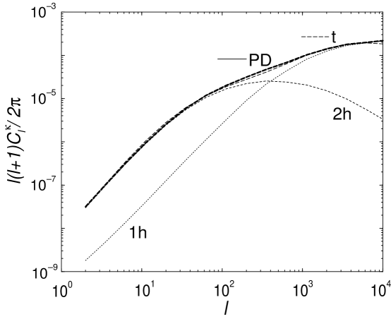
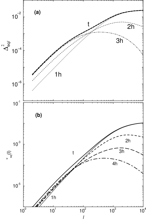
8.2 Convergence

Weak lensing probes the statistical properties of shear field and we can write the deformation matrix that maps $\Delta{\bf x}$ separation vector between source, $s$, and image, $i$, planes, $\Delta{\bf x_{i}}^{s}={\bf A}_{ij}\Delta{\bf x_{j}}^{i}$, as

$${\bf A}_{ij} = \delta_{ij}-\psi_{ij}$$ (168)

$$= \left(\begin{array}[]{cc}1-\kappa-\gamma_{1}&-\gamma_{2}-\omega\\ -\gamma_{2}+\omega&1-\kappa+\gamma_{1}\end{array}\right).$$

Here $\kappa$ is the convergence, responsible for magnification and demagnification, $w$ is the net rotation of the image, and we have separated the components of the shear, $\gamma\equiv\gamma_{1}+i\gamma_{2}$, which translates as a spin-2 field $\gamma=|\gamma|\e^{2i\phi}$ and is a pseudo vector field. The shear components are

$$\gamma_{1} = \frac{1}{2}\left(\psi_{11}-\psi_{22}\right)$$

$$\gamma_{2} = \frac{1}{2}\left(\psi_{12}+\psi_{21}\right)\,$$ (169)

where,

$$\psi_{ij}=2\int_{0}^{r_{s}}dr\frac{d_{A}(r_{d})d_{A}(r_{d}-r_{s})}{d_{A}(r_{s})}\partial_{i}\partial_{j}\Phi\,.$$ (170)

To the smallest order in potential fluctuations, $w\approx 0$ and we can ignore the asymmetry associated with the deformation matrix; thus, $\gamma_{2}=\psi_{12}$ as commonly known.

We can write the convergence using the trace of the deformation matrix with $\kappa=\frac{1}{2}(\psi_{11}+\psi_{22})$:

$$\kappa(\hat{\bf n})=\int_{0}^{r_{s}}dr\,W^{\rm lens}(r)\nabla_{\perp}^{2}\Phi(r,r\hat{\bf n})\,,$$ (171)

where the lensing visibility function for a radial distribution of background sources, $n_{s}(r)$, is

$$W^{\rm lens}(r)=\int_{r}^{r_{s}}dr^{\prime}\frac{d_{A}(r)d_{A}(r^{\prime}-r)}{d_{A}(r^{\prime})}n_{s}(r^{\prime})\,.$$ (172)

Here, $r$ is the comoving radial distance (equation 2) and $d_{A}$ is the angular diameter distance (equation 3).

8.3 Power spectrum

We can write the angular power spectrum of convergence by taking the spherical harmonics

$$\kappa(\hat{\bf n})=\sum\kappa_{lm}Y_{l}^{m}(\hat{\bf n})\,,$$ (173)

with spherical moments of the convergence field defined such that

$$\kappa_{lm} = i^{l}\int\frac{d^{3}{\bf k}}{2\pi^{2}}k_{\perp}^{2}\Phi({\bf k})\int drW(r)j_{l}(kr)Y_{l}^{m}(\hat{{\bf k}})\,,$$

where $W(k,r)$ is the visibility function associated with weak lensing defined in equation (172). Here, we have simplified using the Rayleigh expansion of a plane wave

$$e^{i{\bf k}\cdot\hat{\bf n}r}=4\pi\sum_{lm}i^{l}j_{l}(kr)Y_{l}^{m\ast}(\hat{\bf k})Y_{l}^{m}(\hat{\bf n})\,.$$ (175)

In the small scale limit, only the modes perpendicular to the radial direction contribute to the integral in equation (LABEL:eqn:klmnint) while others are suppressed through near-perfect cancellation of positive and negative oscillations along the line of sight. Thus, we can replace $k_{\perp}\approx k$, which only makes an error of order $\Phi\sim 10^{-5}$. Further, we can use the Poisson equation (equation 29) to relate potential fluctuations to those of density, $k^{2}\Phi(k)=4\pi G\bar{\rho}a^{2}\delta(k)$. These allow us to construct the angular power spectrum of the convergence, defined in terms of the multipole moments, $\kappa_{lm}$, as

$$\left<\kappa_{lm}^{*}\kappa_{l^{\prime}m^{\prime}}\right>=C_{l}^{\kappa}\delta_{ll^{\prime}}\delta_{mm^{\prime}}\,,$$ (176)

to obtain

$$C_{l}=\frac{2}{\pi}\int_{0}^{\infty}k^{2}dkP(k)\int_{0}^{r_{0}}dr_{1}\int_{0}^{r_{0}}dr_{2}W^{\rm lens}(r_{1})W^{\rm lens}(r_{2})j_{l}(kr_{1})j_{l}(kr_{2})\,$$ (177)

where

$$W^{\rm lens}(r)=\frac{3}{2}\Omega_{m}\frac{H_{0}^{2}}{c^{2}}\int_{r}^{r_{0}}dr^{\prime}\frac{d_{A}(r)d_{A}(r^{\prime}-r)}{ad_{A}(r^{\prime})}n_{s}(r^{\prime})\,.$$ (178)

When all background sources are at a distance of $r_{s}$, $n_{s}(r^{\prime})=\delta_{D}(r^{\prime}-r)$, the weight function reduces to

$$W^{\rm lens}(r)=\frac{3}{2}\Omega_{m}\frac{H_{0}^{2}}{c^{2}a}\frac{d_{A}(r)d_{A}(r_{s}-r)}{d_{A}(r_{s})}\,.$$ (179)

In the case of a non-flat geometry, one needs to introduce curvature corrections to the Poisson equation (see, equation 29), and replace the radial Bessel functions, $j_{l}$, with hyperspherical Bessel functions. In the small scale limit, for efficient calculational purposes, we can simplify further by using the Limber, or small angle, approximation [168] where one can neglect the radial component of the Fourier mode ${\bf k}$ compared to the transverse component. Here, we employ a version based on the completeness relation of spherical Bessel functions (see, [54, 122] for details)

$$\int dkk^{2}F(k)j_{l}(kr)j_{l}(kr^{\prime})\approx{\pi\over 2}d_{A}^{-2}\delta^{\rm D}(r-r^{\prime})F(k)\big{|}_{k={l\over d_{A}}}\,,$$ (180)

where the assumption is that $F(k)$ is a slowly-varying function. Under this assumption, the contributions to the power spectrum come only from correlations at equal time surfaces. Finally, we can write the convergence power spectrum as [146, 147]:

$$C^{\kappa}_{l}=\int dr\frac{W^{\rm lens}(r)^{2}}{d_{A}^{2}}P\left(\frac{l}{d_{A}};r\right)\,.$$ (181)

8.4 Relation to Shear Correlations

We can consider the relation between convergence power spectrum and shear correlation functions by considering the Fourier decomposition of the shear field [126] to a gradient-like (E-modes) and curl-like (B-modes) components:

$$\gamma_{1}(\hat{\bf n})\pm i\gamma_{2}(\hat{\bf n})=\int\frac{d^{2}{\bf l}}{(2\pi)^{2}}[\epsilon({\bf l})\pm\beta({\bf l})]\e^{\pm 2i\phi_{l}}\e^{i{\bf l}\cdot\hat{\bf n}}\,,$$ (182)

and consider the correlations between $\langle\gamma_{1}\gamma_{1}\rangle$, $\langle\gamma_{1}\gamma_{2}\rangle$ and $\langle\gamma_{2}\gamma_{2}\rangle$. We can write these correlation functions as

$$\langle\gamma_{1}(\hat{\bf n}_{i})\gamma_{1}(\hat{\bf n}_{j})\rangle = \int\frac{d^{2}{\bf l}}{(2\pi)^{2}}\left[C_{l}^{\epsilon\epsilon}\cos^{2}2\phi_{l}+C_{l}^{\beta\beta}\sin^{2}2\phi_{l}-C_{l}^{\epsilon\beta}\sin 4\phi_{l}\right]\e^{i{\bf l}\cdot(\hat{\bf n}_{i}-\hat{\bf n}_{j})}$$

$$\langle\gamma_{1}(\hat{\bf n}_{i})\gamma_{2}(\hat{\bf n}_{j})\rangle = \int\frac{d^{2}{\bf l}}{(2\pi)^{2}}\left[\frac{C_{l}^{\epsilon\epsilon}}{2}\sin 4\phi_{l}-\frac{C_{l}^{\beta\beta}}{2}\sin 4\phi_{l}+C_{l}^{\epsilon\beta}\cos 4\phi_{l}\right]\e^{i{\bf l}\cdot(\hat{\bf n}_{i}-\hat{\bf n}_{j})}$$

$$\langle\gamma_{2}(\hat{\bf n}_{i})\gamma_{2}(\hat{\bf n}_{j})\rangle = \int\frac{d^{2}{\bf l}}{(2\pi)^{2}}\left[C_{l}^{\epsilon\epsilon}\sin^{2}2\phi_{l}+C_{l}^{\beta\beta}\cos^{2}2\phi_{l}+C_{l}^{\epsilon\beta}\sin 4\phi_{l}\right]\e^{i{\bf l}\cdot(\hat{\bf n}_{i}-\hat{\bf n}_{j})}$$

Using the expansion of $e^{i{\bf l}\cdot(\hat{\bf n}_{i}-\hat{\bf n}_{j})}=\sum_{m}i^{m}J_{m}(l\theta)\e^{im(\phi-\phi_{l})}$, in terms of the magnitude $\theta$ and orientation $\phi$ of vector $\hat{\bf n}_{i}-\hat{\bf n}_{j}$, we write

$$\langle\gamma_{1}\gamma_{1}\rangle_{\theta,\phi} = \int\frac{ldl}{4\pi}\Big{\{}C_{l}^{\epsilon\epsilon}[J_{0}(l\theta)+\cos(4\phi)J_{4}(l\theta)]+C_{l}^{\beta\beta}[J_{0}(l\theta)-\cos(4\phi)J_{4}(l\theta)]$$

$$\quad\quad-2C_{l}^{\epsilon\beta}\sin(4\phi)J_{4}(l\theta)\Big{\}}$$

$$\langle\gamma_{1}\gamma_{2}\rangle_{\theta,\phi} = \int\frac{ldl}{4\pi}\Big{\{}C_{l}^{\epsilon\epsilon}\sin(4\phi)J_{4}(l\theta)-C_{l}^{\beta\beta}\sin(4\phi)J_{4}(l\theta)+C_{l}^{\epsilon\beta}2\cos(4\phi)J_{4}(l\theta)\Big{\}}$$

$$\langle\gamma_{2}\gamma_{2}\rangle_{\theta,\phi} = \int\frac{ldl}{4\pi}\Big{\{}C_{l}^{\epsilon\epsilon}[J_{0}(l\theta)-\cos(4\phi)J_{4}(l\theta)]+C_{l}^{\beta\beta}[J_{0}(l\theta)+\cos(4\phi)J_{4}(l\theta)]$$

$$\quad\quad+2C_{l}^{\epsilon\beta}\sin(4\phi)J_{4}(l\theta)\Big{\}}\,.$$

One can choose an appropriate coordinate system such that measured correlation functions in the coordinate frame are independent of the choice of coordinates; in the above derivation, this is equivalent to setting $\phi=0$ (e.g, [269]). To do this in practice, in analogy with CMB polarization (see, [151]), shear can be measured parallel and perpendicular to the line joining the two points, such that $\hat{\bf n}_{i}-\hat{\bf n}_{j}\parallel\hat{\bf x}$. In such a coordinate system correlation functions reduce to the well known result of [188, 146]:

$$\langle\gamma_{1}\gamma_{1}\rangle_{\theta} = \int\frac{ldl}{4\pi}\left\{C_{l}^{\epsilon\epsilon}[J_{0}(l\theta)+J_{4}(l\theta)]+C_{l}^{\beta\beta}[J_{0}(l\theta)-J_{4}(l\theta)]\right\}$$

$$\langle\gamma_{1}\gamma_{2}\rangle_{\theta} = \int\frac{ldl}{4\pi}2C_{l}^{\epsilon\beta}J_{4}(l\theta)$$

$$\langle\gamma_{2}\gamma_{2}\rangle_{\theta} = \int\frac{ldl}{4\pi}\left\{C_{l}^{\epsilon\epsilon}[J_{0}(l\theta)-J_{4}(l\theta)]+C_{l}^{\beta\beta}[J_{0}(l\theta)+J_{4}(l\theta)]\right\}\,.$$

To the first order, contributions to the shear correlations primarily come from perturbations involving scalars, or gradient-like modes, with $C_{l}^{\epsilon\epsilon}=C_{l}^{\kappa}$ and $C_{l}^{\beta\beta}=C_{l}^{\beta\epsilon}=0$; even if $C_{l}^{\beta\beta}$ contributions are non-zero, the latter $C_{l}^{\beta\epsilon}$ is zero due to parity invariance.

The curl-like modes in shear can be generated by tensor perturbations such as gravity-waves. Since there is no appreciable source of primordial gravity-wave perturbations at late times (see, [154] for a review), it is unlikely that there is a significant contribution to $C_{l}^{\beta\beta}$, except in two cases:

(1) The first order calculation of weak lensing distortion matrix and convergence is that we have implicitly integrated over the unperturbed photon paths (the use of so-called Born approximation, see [14, 234]). Similarly, second-order effects such as lens-lens coupling involving lenses at two-different redshifts can generate a curl-like contribution. With second-order corrections to Born approximation and lens-lens coupling, we can write the deformation matrix associated with weak lensing as

$$A_{ij}=\delta_{ij}-\psi_{ij}^{(1)}-\psi_{ij}^{(2)}\,$$ (186)

with

$$\psi_{ij}^{(2)} = 4\int d\chi^{\prime}\frac{d_{A}(\chi^{\prime})d_{A}(\chi-\chi^{\prime})}{d_{A}(\chi)}$$ (187)

$$\quad\times\int d\chi^{\prime\prime}\frac{d_{A}(\chi^{\prime\prime})d_{A}(\chi^{\prime}-\chi^{\prime\prime})}{d_{A}(\chi^{\prime})}\partial_{i}\partial_{k}\Phi(\chi^{\prime})\partial_{k}\partial_{j}\Phi(\chi^{\prime\prime})\,,$$

due to lens-lens coupling and

$$\psi_{ij}^{(2)} = 4\int d\chi^{\prime}\frac{d_{A}(\chi^{\prime})d_{A}(\chi-\chi^{\prime})}{d_{A}(\chi)}$$ (188)

$$\quad\times\int d\chi^{\prime\prime}d_{A}(\chi^{\prime}-\chi^{\prime\prime})\partial_{i}\partial_{j}\partial_{k}\Phi(\chi^{\prime})\partial_{k}\Phi(\chi^{\prime\prime})\,,$$

due to a correction to Born approximation, respectively [234, 14, 57]. The resulting deformation matrix due to these second-order corrections is asymmetric and results in a contribution to $C_{l}^{\beta\beta}$, as well as a contribution to the net rotation; the latter is equivalent to the Stokes-V contribution in a polarization field or, equivalently, circular polarization.

The Born approximation and lens-lens coupling have been tested in numerical simulations by [134] where they evaluated contribution to the convergence power spectrum resulting from second order effects. Here, the rotational contribution to angular power spectrum, due to lens-lens coupling, is roughly 3 orders of magnitude smaller. In [57], it was shown that the corrections due to the Born approximation is also smaller compared to the first order result that $C_{l}^{\beta\beta}=0$.

(2) The intrinsic correlations between individual background galaxy shapes, due to long range correlations in the tidal gravitational field in which the halos containing galaxies formed, can generate a contribution to $C_{l}^{\beta\beta}$ [60, 110, 37, 175]. The intrinsic correlations have a redshift dependence such that they are significant at low redshifts. In figure 38, we show the resulting $C_{l}^{\epsilon\epsilon}$ and $C_{l}^{\beta\beta}$ power spectra due to ellipticity alignments in background galaxies arising from tidal torques and a comparison to convergence power spectrum associated with ellipticity correlations due to lensing following [175]. In order to avoid the confusion between lensing generated ellipticity correlations vs. tidal torques induced correlations, the results from intrinsic alignment calculations generally indicate that deep surveys are preferred over shallow ones for cosmological purposes. We will return to this issue again based on the non-Gaussian contribution to convergence power spectrum covariance.

Figure 38: The power spectra of lensing convergence (solid) and $C_{l}^{\epsilon\epsilon}$ (dashed) and $C_{l}^{\beta\beta}$ (dot-dashed) due to galaxy ellipticity correlations induced by tidal torques, as a function of redshift. The tidal torques induce significant correlations at low redshifts, while these can be ignored for deep weak lensing surveys with background sources at $z\geq 1$. The figure is from [175].

Figure 39: Moments of the convergence field as a function of top-hat smoothing scale $\sigma$ with (a) Second moment broken into individual contributions and (b) Third moment broken into individual contributions.

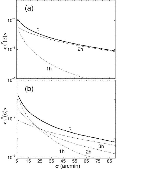
In addition to shear correlations, one can also measure the shear variance, which can be related to the convergence power spectrum by

$$\left<\gamma^{2}(\sigma)\right>\equiv\left<\kappa^{2}(\sigma)\right>={1\over 4\pi}\sum_{l}(2l+1)C_{l}^{\kappa}W_{l}^{2}(\sigma)\,,$$ (189)

where $W_{l}$ are the multipole moments, or Fourier transform in a flat-sky approximation, of the window. In figure 39(a), we choose a window which is a two-dimensional top hat in real space with a window function in multipole space of $W_{l}(\sigma)=2J_{1}(x)/x$ with $x=l\sigma$. As shown, at 5^′ to 90^′ angular scales, most of the contribution to the second moment comes from the double halo correlation term and is dominated by the linear power spectrum instead of the non-linear evolution.

In figure 36(a), we show the convergence power spectrum of the dark matter halos compared with that predicted by the [210] fitting function for the non-linear dark matter power spectrum. The lensing power spectrum due to halos has the same behavior as the dark matter power spectrum. At large angles, $l\mathchar 13358\relax 100$, the correlations between halos dominate. The transition from linear to non-linear is at $l\sim 500$ where halos of mass similar to $M_{\star}(z)$ contribute. The single halo contributions start dominating at $l>1000$. When $l\mathchar 13350\relax$ few thousand, at small scales corresponding to deeply non-linear regime, the shot-noise behavior of the background sources contribute to the convergence power spectrum via a noise term

$$C^{\rm SN}_{l}=\frac{\langle\gamma_{\rm int}^{2}\rangle}{\bar{n}}\,.$$ (190)

Here, $\langle\gamma_{\rm int}\rangle^{1/2}$ is the rms noise per component introduced by intrinsic ellipticities, typically $\sim 0.6$ for best ground based surveys, and $\bar{n}$ is the surface number density of background source galaxies.

Note that the shot-noise term is effectively reduced by the number of independent modes one measures at each multipole. Including the sample variance, the total error expected for a measurement of the power spectrum, as a function of multipole, is

$$\Delta C^{\kappa}_{l}=\sqrt{\frac{2}{f_{\rm sky}(2l+1)}}\left[C^{\kappa}_{l}+C^{\rm SN}_{l}\right]\,.$$ (191)

Here, the first term represents the sample variance under the Gaussian approximation for the convergence field, $\kappa_{lm}$ and is the dominant source of noise at large angular scales. The factor $f_{\rm sky}$, fraction of the sky observed, accounts for the reduction in the number of independent modes under the partial sky coverage. In the absence of noise for an all-sky experiment, at a multipole of $\sim$ 100, the error on the power spectrum due to sample variance is $\sim$ 10% and is usually reduced with binned measurements of the power spectrum in multipole space.

For surveys that reach a limiting magnitude in $R\sim 25$, the surface density is consistent with $\bar{n}\sim 6.9\times 10^{8}$ sr^-1 ($\approx 56$ gal arcmin^-2) [263], such that $C^{\rm SN}_{l}\sim 2.3\times 10^{-10}$. This shot-noise contribution reaches the power due to convergence at multipoles of $\sim$ 2000 and dominates the cosmological weak lensing signal at multipoles thereafter. It is clear that the convergence power spectrum at multipoles of few thousand probe the small scale behavior of the dark matter power spectrum. The presence of significant shot-noise, however, complicate studies that can potentially test assumptions related to large scale structure, such as the stable clustering hypothesis, or the halo model, such as the use of smooth profiles in the presence of substructure seen in numerical simulations.

Figure 40: The bispectrum configuration dependence $R_{l_{1}l_{2}}^{l_{3}}$ as a function of $l_{1}$ and $l_{2}$ with $l_{3}=1000$. Due to triangular conditions associated with $l$’s, only the upper triangular region in $l_{1}$-$l_{2}$ space contribute to the bispectrum.

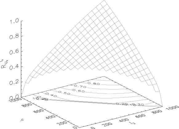
8.5 Bispectrum

Using the spherical harmonic moments of convergence defined in equation (173), the angular bispectrum of the convergence is defined following [54, 265] as

$$\left<\kappa_{l_{1}m_{1}}\kappa_{l_{2}m_{2}}\kappa_{l_{3}m_{3}}\right>=\left(\begin{array}[]{ccc}l_{1}&l_{2}&l_{3}\\ m_{1}&m_{2}&m_{3}\end{array}\right)B_{l_{1}l_{2}l_{3}}^{\kappa}\,.$$ (192)

Here, the quantity in parentheses is the Wigner 3$j$ symbol. Its orthonormality relation implies

$$B_{l_{1}l_{2}l_{3}}^{\kappa}=\sum_{m_{1}m_{2}m_{3}}\left(\begin{array}[]{ccc}l_{1}&l_{2}&l_{3}\\ m_{1}&m_{2}&m_{3}\end{array}\right)\left<\kappa_{l_{1}m_{1}}\kappa_{l_{2}m_{2}}\kappa_{l_{3}m_{3}}\right>\,.$$ (193)

The angular bispectrum, $B_{l_{1}l_{2}l_{3}}^{\kappa}$, contains all the information available in the three-point correlation function, For example, the third moment or the skewness, the collapsed three-point expression of [113] and the equilateral configuration statistic of [81] can all be expressed as linear combinations of the bispectrum terms (see, [90] for explicit expressions).

Similar to our discussion related to the convergence power spectrum, we can write spherical moments of the convergence field defined with respect to the density field as

$$\kappa_{lm}=i^{l}\int\frac{d^{3}{\bf k}}{2\pi^{2}}\delta({\bf k})I_{l}^{\rm lens}(k)Y_{l}^{m}(\hat{{\bf k}})\quad{\rm and}\quad I_{l}^{\rm lens}(k)=\int drW^{\rm lens}(k,r)j_{l}(kr)\,,$$

(194)

where $W(k,r)$ is the source function associated with weak lensing (see equation 178).

The bispectrum can be constructed through

$$\left<\kappa_{l_{1}m_{1}}\kappa_{l_{2}m_{2}}\kappa_{l_{3}m_{3}}\right>=i^{l_{1}+l_{2}+l_{3}}\int\frac{d^{3}{\bf k}_{1}}{2\pi^{2}}\int\frac{d^{3}{\bf k}_{2}}{2\pi^{2}}\int\frac{d^{3}{\bf k}_{3}}{2\pi^{2}}\left<\delta({\bf k}_{1})\delta({\bf k}_{2})\delta({\bf k}_{3})\right>$$

$$\quad\quad\times I_{l}^{\rm lens}(k_{1})I_{l}^{\rm lens}(k_{2})I_{l}^{\rm lens}(k_{3})Y_{l_{1}}^{m_{1}}(\hat{{\bf k}_{1}})Y_{l_{2}}^{m_{2}}(\hat{{\bf k}_{2}})Y_{l_{3}}^{m_{3}}(\hat{{\bf k}_{3}})\,,$$ (195)

and can be simplified further by using the bispectrum of density fluctuations to write the convergence bispectrum as

$$B^{\kappa}_{l_{1}l_{2}l_{3}} = \sum_{m_{1}m_{2}m_{3}}\left(\begin{array}[]{ccc}l_{1}&l_{2}&l_{3}\\ m_{1}&m_{2}&m_{3}\end{array}\right)\left<\kappa_{l_{1}m_{1}}\kappa_{l_{2}m_{2}}\kappa_{l_{3}m_{3}}\right>$$ (198)

$$= \sqrt{\frac{\prod_{i=1}^{3}(2l_{i}+1)}{4\pi}}\left(\begin{array}[]{ccc}l_{1}&l_{2}&l_{3}\\ 0&0&0\end{array}\right)b_{l_{1},l_{2},l_{3}}\,,$$ (201)

with

$$b_{l_{1},l_{2},l_{3}}=\frac{2^{3}}{\pi^{3}}\int k_{1}^{2}dk_{1}\int k_{2}^{2}dk_{2}\int k_{3}^{2}dk_{3}B(k_{1},k_{2},k_{3})$$

$$\times I^{\rm lens}_{l_{1}}(k_{1})I^{\rm lens}_{l_{2}}(k_{2})I^{\rm lens}_{l_{3}}(k_{3})\int x^{2}dxj_{l_{1}}(k_{1}x)j_{l_{2}}(k_{2}x)j_{l_{3}}(k_{3}x)\,.$$

In general, the calculation of $b_{l_{1},l_{2},l_{3}}$ involves seven integrals involving the mode coupling integral and three integrals involving distances and Fourier modes, respectively. We can simplify further by employing the Limber approximation similar to our derivation of the power spectrum. Applying equation (180) to the integrals involving $k_{1}$, $k_{2}$ and $k_{3}$ allows us to write the angular bispectrum of lensing convergence as

$$B_{l_{1}l_{2}l_{3}}^{\kappa} = \sqrt{\prod_{i=1}^{3}(2l_{i}+1)\over 4\pi}\left(\begin{array}[]{ccc}l_{1}&l_{2}&l_{3}\\ 0&0&0\end{array}\right)\int dr{[W^{\rm lens}(r)]^{3}\over d_{A}^{4}}B\left({l_{1}\over d_{A}},{l_{2}\over d_{A}},{l_{3}\over d_{A}};r\right)\,.$$ (205)

Through angular momentum selection rules, the Wigner-3$j$ symbol restricts $l_{i}$ to form a triangle such that $l_{i}\leq|l_{j}-l_{k}|$. Additional properties of the Wigner 3$j$ symbol can be found in the Appendix of [54].

The more familiar flat-sky bispectrum is [55, 120]:

$$B^{\kappa}({\bf l}_{1},{\bf l}_{2},{\bf l}_{3})=\int dr{[W^{\rm lens}(r)]^{3}\over d_{A}^{4}}B\left({{\bf l}_{1}\over d_{A}},{{\bf l}_{2}\over d_{A}},{{\bf l}_{3}\over d_{A}};r\right)\,,$$ (207)

where ${\bf l}_{i}$ are now two-dimensional vectors. In the case of the flat-sky bispectrum, the Wigner 3$j$ symbol in the all sky expression becomes a triangle equality relating the two-dimensional vectors. The implication is that the triplet $(l_{1},l_{2},l_{3})$ can be considered to contribute to the triangle configuration of ${\bf l}_{1},{\bf l}_{3},{\bf l}_{3}=-({\bf l}_{1}+{\bf l}_{2})$ where the multipole number is taken as the length of the vector. The correspondence between the all-sky derivation, equation (LABEL:eqn:kappabispectrum), and the flat-sky approximation, equation (207), can be noted by expanding the delta function involved with ${\bf l}_{1}+{\bf l}_{2}+{\bf l}_{3}=0$ [120].

In the flat-sky case, we can generalize our result for a any n-point Fourier space correlation as

$$P_{N}^{\kappa}({\bf l}_{1},...,{\bf l}_{N})=\int dr{[W^{\rm lens}(r)]^{N}\over d_{A}^{(2N-2)}}P_{N}\left({{\bf l}_{1}\over d_{A}},...,{{\bf l}_{N}\over d_{A}};r\right)\,,$$ (208)

where vectors ${\bf l}_{1}+...+{\bf l}_{N}=0$.

Similar to the density field bispectrum, we define

$$\Delta^{2}_{{\rm eq}l}=\frac{l^{2}}{2\pi}\sqrt{B^{\kappa}_{lll}}\,,$$ (209)

involving equilateral triangles in $l$-space. In figure 37(a), we show $\Delta^{2}_{{\rm eq}l}$. The general behavior of the lensing bispectrum can be understood through the individual contributions to the density field bispectrum: at small multipoles, the triple halo correlation term dominates, while at high multipoles, the single halo term dominates. The double halo term contributes at intermediate $l$’s corresponding to angular scales of a few tens of arcminutes. In figure 40, we plot the configuration dependence

$$R_{l_{1}l_{2}}^{l_{3}}=\frac{l_{1}l_{2}}{2\pi}\frac{\sqrt{B^{\kappa}_{l_{1}l_{2}l_{3}}}}{\Delta^{2}_{{\rm eq}l}}$$ (210)

as a function of $l_{1}$ and $l_{2}$ when $l_{3}=1000$. The surface, and associated contour plot, shows the contribution to the bispectrum from triangular configurations in $l$-space relative to that from the equilateral configuration. Because of the triangular conditions associated with $l$’s, only upper triangular region of $l_{1}$-$l_{2}$ space contribute to the bispectrum. The symmetry about the $l_{1}=l_{2}$ line is due to the intrinsic symmetry associated with the bispectrum. Although the weak lensing bispectrum peaks for equilateral configurations, the configuration dependence is weak. In the case of dark matter bispectrum, it is now known that the halo model somewhat overestimates the configuration dependence due to the spherical assumption for halos [236]. This overestimate should also be present in the projected dark matter statistics such as lensing convergence bispectrum.

As discussed in the case of the second moment, it is likely that the first measurements of higher order correlations in lensing would be through real space statistics. Thus, in addition to the bispectrum, we also consider skewness, which is associated with the third moment of the smoothed map (c.f. equation. [189])

$$\left<\kappa^{3}(\sigma)\right> = {1\over 4\pi}\sum_{l_{1}l_{2}l_{3}}\sqrt{\prod_{i=1}^{3}(2l_{i}+1)\over 4\pi}\left(\begin{array}[]{ccc}l_{1}&l_{2}&l_{3}\\ 0&0&0\end{array}\right)B_{l_{1}l_{2}l_{3}}^{\kappa}W_{l_{1}}(\sigma)W_{l_{2}}(\sigma)W_{l_{3}}(\sigma)\,.$$ (213)

One can then construct the skewness as

$$S_{3}(\sigma)=\frac{\left<\kappa^{3}(\sigma)\right>}{\left<\kappa^{2}(\sigma)\right>^{2}}\,,$$ (215)

where $\left<\kappa^{2}(\sigma)\right>^{2}$ is the second moment of the convergence field defined in equation (189).

Figure 41: The skewness, $S_{3}(\sigma)$, as a function of angular scale. The filled symbols indicate the mean and variance computed from a set of $\kappa$ planes generated in particle-mesh (PM) simulations by [289]. Under the halo model, shown here is the skewness with varying maximum mass used in the calculation (solid lines ranging from 10¹⁴ to 10¹⁶ M${}_{\hbox{$\odot$}}$). For comparison, we also show skewness values as predicted by hyper-extended perturbation theory (HEPT) and second-order perturbation theory (PT). Figure is reproduced based on [289] and [55].

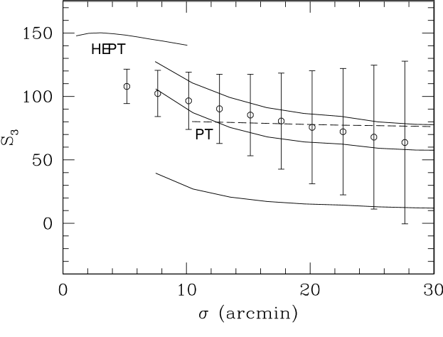
In figure 41, we plot the skewness based on the halo model. Here, we show skewness as a function of maximum mass, ranging from $10^{14}$ to $10^{16}$ M${}_{\hbox{$\odot$}}$ (from increasing values of skewness). The assumption is that certain surveys, either by design in the case of so-called blank-fields or by chance, will not contain massive halos in the universe. Thus, by arbitrarily cutting off the maximum mass when integrating over the mass function, one can estimate how the statistics are sensitive to the presence of the massive and rare objects in the universe. Our total maximum skewness agrees with what is predicted by numerical particle mesh simulations [289] and yields a value of $\sim$ 116 at 10^′. However, it is lower than predicted by HEPT arguments and simulations of [134], which suggest a skewness of $\sim$ 140 at angular scales of 10^′ [128]. The HEPT prediction generally overpredicts skewness as it is extended to the mildly non-linear regime of clustering, where contributions to the skewness come from at arcminute scales, from the deeply non-linear regime, corresponding to angular scales of few arcseconds, where it is expected to be valid. The skewness based on second-order PT [14] is lower than the maximum skewness predicted by halo calculation, and by construction, agrees with the skewness in the linear regime.

The effect of maximum mass on the skewness is interesting. When the maximum mass is decreased to $10^{15}$ M${}_{\hbox{$\odot$}}$ from the maximum mass value where skewness saturates ($\sim 10^{16}$ M${}_{\hbox{$\odot$}}$), the skewness decreases from $\sim$ 116 to 98 at an angular scale of 10^′, though the convergence power spectrum only changes by less than few percent when the same change on the maximum mass used is made. When the maximum mass used in the calculation is $10^{14}$ M${}_{\hbox{$\odot$}}$, the skewness at 10^′ is $\sim 40$, which is roughly a factor of 4 decrease in the skewness from the total.

Thus, the absence of rare and massive halos in observed fields will certainly bias the skewness measurement from the cosmological mean, which has been suggested as a probe of the cosmological matter density given that $S_{3}\propto\Omega_{m}^{-0.8}$ [14]. One, therefore, needs to exercise caution in using the skewness to constrain cosmological models [128]. Still, this does not mean that non-Gaussianity measured in small fields, where there is likely to be a significant bias due to the lack of massive halos, will be useless. With the halo approach, one can calculate the expected skewness given some information related to the mass distribution of halos within the observed fields. This knowledge may come externally, such as through X-ray and Sunyaev-Zel’dovich measurements or internally from lensing data themselves, independent of cosmology. Alternatively, if cosmology is assumed, one can also used non-Gaussian information from weak lensing to constrain some aspect of the large scale structure halo mass distribution, such as the high mass end of the mass function.

8.6 Weak Gravitational lensing Covariance

For the purpose of this calculation, we assume that upcoming weak lensing convergence power spectrum will measure binned logarithmic band powers at several $l_{i}$’s in multipole space with bins of thickness $\delta l_{i}$.

$${\cal C}_{i}=\int_{{\rm s}i}{d^{2}l\over{A_{{\rm s}i}}}\frac{l^{2}}{2\pi}\kappa(\bf l)\kappa(-\bf l)\,,$$ (216)

where $A_{\rm s}(l_{i})=\int d^{2}l$ is the area of the two-dimensional shell in multipole and can be written as $A_{\rm s}(l_{i})=2\pi l_{i}\delta l_{i}+\pi(\delta l_{i})^{2}$.

We can now write the signal covariance matrix as

$$C_{ij} = {1\over A}\left[{(2\pi)^{2}\over A_{{\rm s}i}}2{\cal C}_{i}^{2}+T^{\kappa}_{ij}\right]\,,$$ (217)

$$T^{\kappa}_{ij} = \int{d^{2}l_{i}\over A_{{\rm s}i}}\int{d^{2}l_{j}\over A_{{\rm s}j}}{l_{i}^{2}l_{j}^{2}\over(2\pi)^{2}}T^{\kappa}({\mathbf{l}}_{i},-{\mathbf{l}}_{i},{\mathbf{l}}_{j},-{\mathbf{l}}_{j})\,,$$ (218)

where $A=4\pi f_{\rm sky}$ is the area of the survey in steradian, when the fraction of sky covered is $f_{\rm sky}$. Again the first term is the Gaussian contribution to the sample variance and the second term is the non-Gaussian contribution. A realistic survey will also have shot noise variance due to the finite number of source galaxies in the survey. Note that in the Gaussian limit with $T^{\kappa}_{ij}=0$, when $\delta l_{i}=1$, equation (218) reduces to $(\Delta C^{\kappa}_{l})^{2}$ given in equation (191).

Following equation (208), the convergence trispectrum is related to the density trispectrum by the projection [235, 56]

$$T^{\kappa} = \int dr\frac{W(r)^{4}}{d_{A}^{6}}T\left(\frac{{\mathbf{l}}_{1}}{d_{A}},\frac{{\mathbf{l}}_{2}}{d_{A}},\frac{{\mathbf{l}}_{3}}{d_{A}},\frac{{\mathbf{l}}_{4}}{d_{A}};r\right)\,,$$ (219)

with the weight function defined in equation (178) and ${\bf l}_{4}=-({\bf l}_{1}+{\bf l}_{2}+{\bf l}_{3})$.

Note that the configurations, in Fourier space, that contribute to the power spectrum covariance has the form of parallelograms with ${\bf l}_{2}=-{\bf l}_{1}$ and ${\bf l}_{4}=-{\bf l}_{3}$. Thus, it is useful to consider the behavior of the trispectrum for such configurations. In figure 37(b), we show the scaled trispectrum

$$\Delta^{\kappa}_{\rm sq}(l)=\frac{l^{2}}{2\pi}T^{\kappa}({\bf l},-{\bf l},{\bf l}_{\perp},-{\bf l}_{\perp})^{1/3}\,.$$ (220)

where $l_{\perp}=l$ and ${\bf l}\cdot{\bf l}_{\perp}=0$. The projected lensing trispectrum again shows the same behavior as the density field trispectrum with similar conditions on ${\bf k}_{i}$’s.

We can now use this trispectrum to study the contributions to the covariance, which is what we are primarily concerned here. In figure 42a, we show the fractional error,

$${\Delta{\cal C}_{i}\over{\cal C}_{i}}\equiv{\sqrt{C_{ii}}\over{\cal C}_{i}}\,,$$ (221)

for bands $l_{i}$ given in Table 3 following the binning scheme used by [289] on $6^{\circ}\times 6^{\circ}$ fields.

Figure 42: The fractional errors in the measurements of the convergence band powers. In (a), we show the fractional errors under the Gaussian approximation, the full halo description, the Gaussian plus single halo term, and the Gaussian plus shot noise term (see equation 228). As shown, the additional variance can be modeled with the single halo piece while shot noise generally becomes dominant before non-Gaussian effects become large. In (b), we compare the halo model with simulations from [289] (1999). The decrease in the variance at small $l$ in the simulations is due to the conversion of variance to covariance by the finite box size of the simulations.

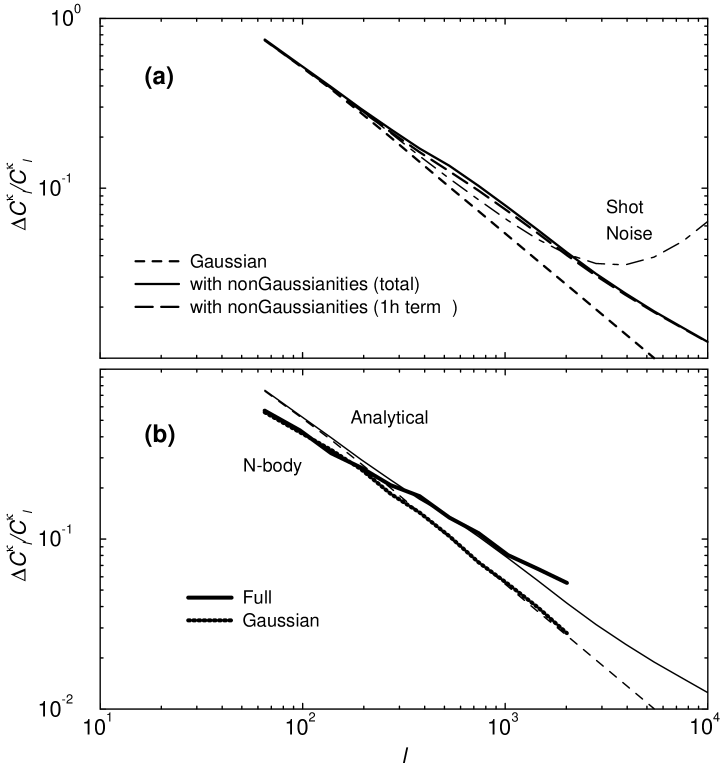
The dashed line compares that with the Gaussian errors, involving the first term in the covariance (equation 218). At multipoles of a few hundred and greater, the non-Gaussian term begins to dominate the contributions. For this reason, the errors are well approximated by simply taking the Gaussian and single halo contributions. In figure 42(b), we compare these results with those of the [289] simulations. The decrease in errors from the simulations at small $l$ reflects finite box effects that convert variance to covariance as the fundamental mode in the box becomes comparable to the bandwidth.

The correlation between the bands is given by

$$\hat{C}_{ij}\equiv\frac{C_{ij}}{\sqrt{C_{ii}C_{jj}}}\,.$$ (222)

In table 3, we compare the halo predictions to the simulations by [289]. The upper triangle here is the correlations under the halo approach, while the lower triangle shows the correlations found in numerical simulations. The correlations along individual columns increase, as one goes to large $l$’s or small angular scales, consistent with simulations. In figure 43, we show the correlation coefficients with (a) and without (b) the Gaussian contribution to the diagonal.

Figure 43: (a) The correlation coefficient, $\hat{C}_{ij}$ as a function of the multipole $l_{i}$ with $l_{j}$ as shown in the figure. We show the correlations calculated with the full halo model and also with only the single halo term for $l_{j}=77072$. In (b), we show the non-Gaussian correlation coefficient $\hat{C}_{ij}^{\rm NG}$, which only involves the trispectrum (see, equation 223). The transition to full correlation is due to the domination of the single halo contribution.

Table 3:

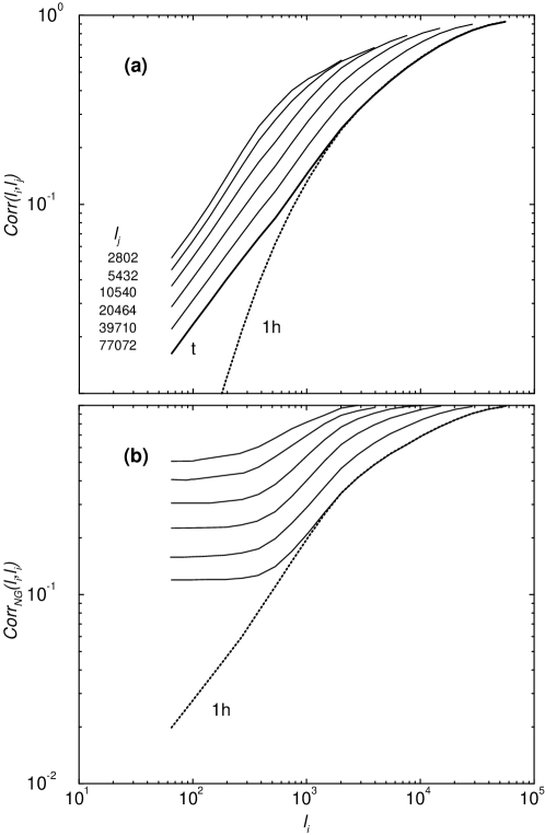
Weak Lensing Convergence Power Spectrum Correlations
$\ell_{\rm bin}$ 97 138 194 271 378 529 739 1031 1440 2012 97 1.00 0.04 0.05 0.07 0.08 0.09 0.09 0.09 0.08 0.08 138 (0.26) 1.00 0.08 0.10 0.11 0.12 0.12 0.12 0.11 0.11 194 (0.12) (0.31) 1.00 0.14 0.17 0.18 0.18 0.17 0.16 0.15 271 (0.10) (0.21) (0.26) 1.00 0.24 0.25 0.25 0.24 0.22 0.21 378 (0.02) (0.09) (0.24) (0.38) 1.00 0.33 0.33 0.32 0.30 0.28 529 (0.10) (0.14) (0.28) (0.33) (0.45) 1.00 0.42 0.40 0.37 0.35 739 (0.12) (0.16) (0.17) (0.34) (0.38) (0.50) 1.00 0.48 0.45 0.42 1031 (0.15) (0.18) (0.15) (0.27) (0.33) (0.48) (0.54) 1.00 0.52 0.48 1440 (0.18) (0.15) (0.19) (0.19) (0.32) (0.36) (0.53) (0.57) 1.00 0.54 2012 (0.19) (0.22) (0.16) (0.32) (0.27) (0.46) (0.50) (0.61) (0.65) 1.00

NOTES.—Covariance of the binned power spectrum when sources are at a redshift of 1. Upper triangle displays the covariance found under the halo model. Lower triangle (parenthetical numbers) displays the covariance found in numerical simulations by [289]. To be consistent with these simulations, we use the same binning scheme as the one used there.

We show in figure 43(a) the behavior of the correlation coefficient between a fixed $l_{j}$ as a function of $l_{i}$. When $l_{i}=l_{j}$ the coefficient is 1 by definition. Due to the presence of the dominant Gaussian contribution at $l_{i}=l_{j}$, the coefficient has an apparent discontinuity between $l_{i}=l_{j}$ and $l_{i}=l_{j-1}$ that decreases as $l_{j}$ increases and non-Gaussian effects dominate.

To better understand this behavior it is useful to isolate the purely non-Gaussian correlation coefficient

$$\hat{C}^{\rm NG}_{ij}=\frac{T_{ij}}{\sqrt{T_{ii}T_{ij}}}\,.$$ (223)

As shown in figure 43(b), the coefficient remains constant for $l_{i}\ll l_{j}$ and smoothly increases to unity across a transition scale that is related to where the single halo terms starts to contribute. A comparison of figure 43(b) and 37(b), shows that this transition happens around $l$ of few hundred to 1000. Once the power spectrum is dominated by correlations in single halos, the fixed profile of the halos will correlate the power in all the modes. The multiple halo terms on the other hand correlate linear and non-linear scales but at a level that is generally negligible compared with the Gaussian variance.

Note that the behavior seen in the halo based covariance, however, is not present when the covariance is calculated with hierarchical arguments for the trispectrum (see, [235]). With hierarchical arguments, which are by construction only valid in the deeply non-linear regime, one predicts correlations which are, in general, constant across all scales and shows no decrease in correlations between very small and very large scales. Such hierarchical models also violate the Schwarz inequality with correlations greater than 1 between large and small scales (e.g., [235, 104]). The halo model, however, shows a decrease in correlations similar to numerical simulations suggesting that the halo model, at least qualitatively, provides a better approach to studying non-Gaussian correlations in the translinear regime.

8.6.1 Scaling Relations

To better understand how the non-Gaussian contribution scale with our assumptions, we can consider the ratio of non-Gaussian variance to the Gaussian variance

$$\frac{C_{ii}}{C_{ii}^{\rm G}}=1+R\,,$$ (224)

with

$$R\equiv\frac{A_{si}T_{ii}^{\kappa}}{(2\pi)^{2}2C_{i}^{2}}\,.$$ (225)

Under the assumption that contributions to lensing convergence can be written through an effective distance $r_{\star}$, at half the angular diameter distance to background sources, and a width $\Delta r$ for the lensing window function, the ratio of lensing convergence trispectrum and power spectrum contribution to the variance can be further simplified to

$$R\sim\frac{A_{si}}{(2\pi)^{2}V_{\rm eff}}\frac{\bar{T}(r_{\star})}{2\bar{P}^{2}(r_{\star})}\,.$$ (226)

Since the lensing window function peaks at $r_{\star}$, we have replaced the integral over the window function of the density field trispectrum and power spectrum by its value at the peak. This ratio shows how the relative contribution from non-Gaussianities scale with survey parameters: (a) increasing the bin size, through $A_{si}$ ($\propto\delta l$), leads to an increase in the non-Gaussian contribution linearly, (b) increasing the source redshift, through the effective volume of lenses in the survey ($V_{\rm eff}\sim r_{\star}^{2}\Delta r$), decreases the non-Gaussian contribution, while (c) the growth of the density field trispectrum and power spectrum, through the ratio $\bar{T}/\bar{P}^{2}$, decreases the contribution as one moves to a higher redshift. The volume factor quantifies the number of foreground halos in the survey that effectively act as gravitational lenses for background sources; as the number of such halos is increased, the non-Gaussianities are reduced by the central limit theorem.

In figure 44, we summarize our results as a function of source redshift with $l_{i}\sim 10^{2},10^{3}$ and 10⁴ and setting the bin width such that $A_{s}(l_{i})\sim l_{i}^{2}$, or $\delta l\sim l$. As shown, increasing the source redshift leads to a decrease in the non-Gaussian contribution to the variance. The prediction based on the simplifications in equation (226) tend to overestimate the non-Gaussianity at lower redshifts while underestimates it at higher redshifts, though the exact transition depends on the angular scale of interest; this behavior can be understood due to the fact that we do not consider the full lensing window function but only the contributions at an effective redshift, midway between the observer and sources.

In order to determine whether its the increase in volume or the decrease in the growth of structures that lead to a decrease in the relative importance of non-Gaussianities as one moves to a higher source redshift, we calculated the non-Gaussian to Gaussian variance ratio under the halo model for several source redshifts and survey volumes. Up to source redshifts $\sim$ 1.5, the increase in volume decreases the non-Gaussian contribution significantly. When surveys are sensitive to sources at redshifts beyond 1.5, the increase in volume becomes less significant and the decrease in the growth of structures begin to be important in decreasing the non-Gaussian contribution. Since, in the deeply non-linear regime, $\bar{T}/\bar{P}^{2}$ scales with redshift as the cube of the growth factor, this behavior is consistent with the overall redshift scaling of the volume and growth.

The importance of the non-Gaussianity to the variance also scales linearly with bin width. As one increases the bin width the covariance induced by the non-Gaussianity manifests itself as increased variance relative to the Gaussian case. The normalization of $R$ is therefore somewhat arbitrary in that it depends on the binning scheme, i.e. $R\ll 1$ does not necessarily mean non-Gaussianity can be entirely neglected when summing over all the bins. The scaling with redshift and the overall scaling of the variance with the survey area $A$ is not. One way to get around the increased non-Gaussianity associated with shallow surveys, is to have it sample a wide patch of sky since $C_{ii}\propto(1+R)/A$. This relation tells us the trade off between designing an survey to go wide instead of deep. One should bear in mind though that not only will shallow surveys have decreasing number densities of source galaxies and hence increasing shot noise, they will also suffer more from the decreasing amplitude of the signal itself and the increasing importance of systematic effects, including the intrinsic correlations of galaxy shapes (e.g., [37, 60, 110]). These problems tilt the balance more towards deep but narrow surveys than the naive statistical scaling would suggest.

Figure 44: The ratio of non-Gaussian to Gaussian contributions, $R$, as a function of source redshift ($z_{s}$). The solid lines are through the exact calculation (equation 225) while the dotted lines are using the approximation given in equation (226). Here, we show the ratio $R$ for three multipoles corresponding to large, medium and small angular scales. The multipole binning is kept constant such that $\delta l\sim l$. Decreasing this bin size will linearly decrease the value of $R$.

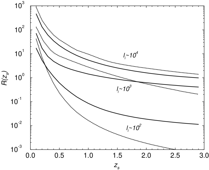
8.6.2 The effect of non-Gaussianities

With steady improvements in the observational front, it is likely that weak lensing will eventually reach its full ability as a complimentary probe of cosmological parameters when compared to angular power spectrum of CMB anisotropies (see, e.g., [121]). Thus, for a proper interpretation of observational measurements of lensing convergence power spectrum or shear correlation functions, it will be essential to include the associated full covariance or error matrix in upcoming analyses. In the absence of many fields where the covariance can be estimated directly from the data, the halo model provides a useful, albeit model dependent, quantification of the covariance. As a practical approach one could imagine taking the variances estimated from the survey under a Gaussian approximation, but which accounts for uneven sampling and edge effects [126], and scaling it up by the non-Gaussian to Gaussian variance ratio of the halo model along with inclusion of the band power correlations. Additionally, it is in principle possible to use the expected correlations from the halo model to decorrelate individual band power measurements, similar to studies involving CMB temperature anisotropy and galaxy power spectra (e.g., [103, 105]).

The resulting non-Gaussian effects on cosmological parameter estimation was discussed in [56]. In [121], the potential of wide-field lensing surveys to measure cosmological parameters was investigated using the Gaussian approximation of a diagonal covariance and Fisher matrix techniques. The Fisher matrix is simply a projection of the covariance matrix, ${\bf C}$, onto the basis of cosmological parameters $p_{i}$

$${\bf F}_{\alpha\beta}=\sum_{ij}{\partial{\cal C}_{i}\over\partial p_{\alpha}}({\bf C}_{\rm tot}^{-1})_{ij}{\partial{\cal C}_{j}\over\partial p_{\beta}}\,,$$ (227)

where the total covariance includes both the signal and noise covariance. Under the approximation of Gaussian shot noise, this reduces to replacing $C^{\kappa}_{l}\rightarrow C^{\kappa}_{l}+C^{\rm SN}_{l}$ in the expressions leading up to the covariance equation (218). In the case where non-Gaussian contribution to the covariance is ignored, equation (227) reduces to [121, 48]

$${\bf F}_{\alpha\beta}=\sum_{l=l_{\rm min}}^{l_{\rm max}}\frac{f_{\rm sky}(l+1/2)}{(C^{\kappa}_{l}+C^{\rm SN}_{l})^{2}}\frac{\partial C^{\kappa}_{l}}{\partial p_{\alpha}}\frac{\partial C^{\kappa}_{l}}{\partial p_{\beta}}\,.$$ (228)

Under the approximation that there are a sufficient number of modes in the band powers that the distribution of power spectrum estimates is approximately Gaussian, the Fisher matrix quantifies the best possible errors on cosmological parameters that can be achieved by a given survey. In particular $F^{-1}$ is the optimal covariance matrix of the parameters and $(F^{-1})_{ii}^{1/2}$ is the optimal error on the $i$th parameter.

For a cosmological model involving a set of 5 parameters, $\Omega_{\Lambda}$, normalization of the power spectrum, $\Omega_{K}=1-\Omega_{m}-\Omega_{\Lambda}$, $n_{s}$ and $\Omega_{m}h^{2}$, Cooray & Hu [55] found that non-Gaussianities increase the uncertainties of each of the 5 parameters determined from an all-sky experiment down to the 25th magnitude, and assuming all sources at a redshift of $\sim$ 1, by about $\sim$ 10 to 15%. In the case of weak lensing, the shot-noise due to finite number of background sources and their intrinsic ellipticity becomes the dominant error before the non-Gaussian effects dominate over the Gaussian noise. Thus, for the above assumed depth and redshift, the non-Gaussian effect on cosmological parameters is some what insignificant. For certain planned deeper surveys with better imaging, such as planned surveys with Large-Aperture Synoptic Telescope (LSST; [281]), the shot-noise term will be subdominant and the non-Gaussian contributions may be more important for a precise determination of the cosmological parameters. As discussed with scaling relations, § 8.6.1, the intrinsic non-Gaussian contribution to the onset of non-linearity decreases with increasing survey depth, and thus, deeper surveys are in fact preferred over shallow ones for the purposes of cosmological lensing work.

8.7 The Galaxy-Mass Cross-Correlation

Figure 45: The SDSS galaxy-mass cross-correlation using galaxy-shear correlation function. We show the halo model prediction with a solid line. The data are from [83].

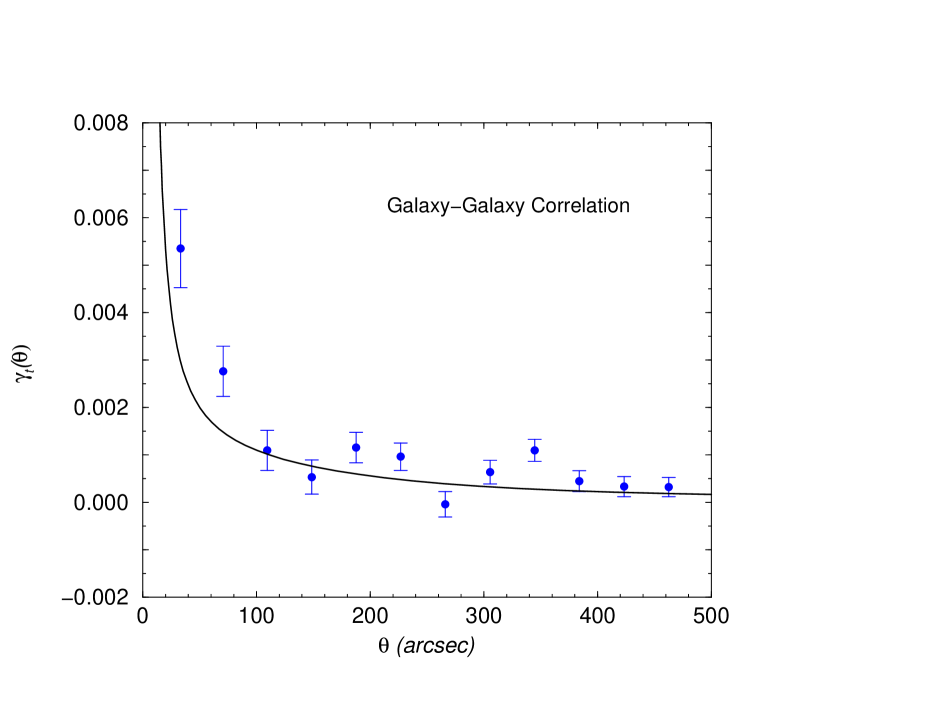
Our description for the galaxy power spectrum, see § 6, allows us to extend the discussion to also consider the cross-correlation between galaxies and mass. Such a cross-power spectrum can be probed through two independent methods: (1) the weak lensing tangential shear-galaxy correlation function and (2) the foreground-background source correlation function. As we find later, these two correlations probe different scales in the galaxy-mass power spectrum.

8.8 Shear-Galaxy correlation

The shear-galaxy correlation function can be constructed by correlating tangential shear of background galaxies surrounding foreground galaxies. The assumption is that these foreground galaxies trace the mass distribution along the line of sight to background sources. Here, observations involve the mean tangential shear due to gravitational lensing which is related to convergence through

$$\left<\gamma_{t}(\theta)\right>=-\frac{1}{2}\frac{d\bar{\kappa}(\theta)}{d{\rm ln}\theta}\,,$$ (229)

where $\bar{\kappa}(\theta)$ is the mean convergence within a circular radius of $\theta$ [148, 267, 99].

Since the shear, averaged over a circular aperture, is correlated with foreground galaxy positions, one essentially probes the galaxy-mass correlation discussed in § 8.7 such that

$$\bar{\kappa}(\theta)=\int drW^{\rm lens}(r)W^{\rm gal}(r)\int dkkP_{{\rm gal}-\rm DM}(k)\frac{2J_{1}(kd_{A}\theta)}{kd_{A}\theta}\,.$$ (230)

Following equation (229), we can write the mean tangential shear involved with galaxy-galaxy lensing as

$$\left<\gamma_{t}(\theta)\right>=\int drW^{\rm lens}(r)W^{\rm gal}(r)\int dkkP_{{\rm gal}-\rm DM}(k)J_{2}(kd_{A}\theta)\,.$$ (231)

Here, $W^{\rm lens}$ is the lensing window function introduced in equation (178), while $W^{\rm gal}$ is the normalized redshift distribution of foreground galaxies. Note that, in general, $W^{\rm lens}$ involves the redshift distribution of background sources beyond the simple single source redshift assumption we have considered in prior calculations.

The highest signal-to-noise measurement yet of tangential lensing correlation around foreground galaxies comes from the Sloan Digital Sky Survey [83]. We compare these measurements with a prediction based on the halo model in figure 45. Here, for simplicity, we take the same description for galaxy number counts as introduced in § 6, and calculate the galaxy-dark matter correlation function following equations (131). In calculating the expected correlation function, we have used the expected redshift distributions for foreground and background galaxies in the Sloan samples. The observed measurements shown in figure 45 comes from the Sloan survey for field galaxies; tangential shear around a selected sample of 42 foreground galaxy clusters in Sloan data were recently presented by [248]. Traditionally, the galaxy-galaxy lensing correlation function, similar to the above, was interpreted by a mass and a size distribution for foreground galaxies with foreground galaxies generally assumed to be distributed randomly. This, or similar approaches, allow constraints on certain galaxy properties such as mass and size (see, [83] for details).

The halo model provides an alternative, and perhaps an improved, description consistent with our basic ideas of large scale structure: since galaxies effectively trace the dark matter halos and it is the dark matter that is mostly responsible for the tangential lensing of background sources, the constraints on mass and size effectively applies to halos that galaxies reside in. If field galaxies are simply selected as foreground sources, then, the constraint on mass and size applies to the dark matter halo of the sample, each of which contains a single galaxy. If the foreground sample contains contributions from a wide variety of dark matter halo mass scales, then more than one galaxy can reside in dark matter halos at the high mass end and a simple interpretation may not be possible. Additionally, since halos distribute the large scale structure, one should account for the clustering component, i.e.,. the 2-halo term of the dark matter-galaxy correlation function, when extracting statistical properties related to individual halos that contribute along the line of sight. As shown in figure 45, the total halo model prediction, both due to individual halos and their clustering, is consistent with observed measurements; the correlation at largest angular scales is due to the intrinsic clustering of halos and cannot be simply interpreted as a large extent for the dark matter halos. A more thorough study of the weak lensing shear-galaxy cross-correlation, under the halo model, is available in [99] and we refer the reader to this paper for further details.

Figure 46: The window functions involved with the projection of galaxy-mass power spectrum in producing the tangential shear-galaxy correlation ($J_{2}$) and the foreground-background galaxy correlation ($J_{0}$). Note that the tangential shear-galaxy correlation probes smaller physical scales in the galaxy-mass power spectrum and are, thus, more sensitive to the non-linear aspect of this correlation function, such as the single-halo contribution.

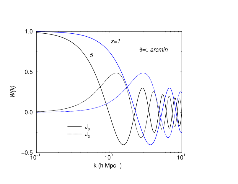
8.9 Foreground-background source correlation

The second observational probe of the galaxy-mass correlation function comes from the clustering of background sources around foreground objects. One can construct a power spectrum by simply counting the number of objects, such as quasars or X-ray sources, surrounding a sample of foreground sources, such as galaxies. The dependence on the correlation comes from the fact that foreground sources trace the mass density field which can potentially affect the number counts of background sources by the weak lensing effect.

To understand this correlation, we can consider a sample of background sources whose number counts can be written as

$$N(s)=N_{0}s^{-\alpha}\,$$ (232)

where $s$ is the flux and $\alpha$ is the slope of number counts. Due to lensing, when the amplification involved is $\mu$, one probes to a lower flux limit $s/\mu$ while the total number of sources are reduced by another factor $\mu$; the latter results from the decrease in volume such that the total surface brightness is conserved in lensing. Thus, in the presence of lensing, number counts are changed to

$$N(s) = \frac{N_{0}}{\mu}\left(\frac{s}{\mu}\right)^{-\alpha}$$ (233)

$$= N_{0}s^{-\alpha}\mu^{\alpha-1}\,.$$

In the limit of weak lensing, as more appropriate for the large scale structure, $\mu\approx(1+2\kappa)$ where convergence $\kappa$ was defined in equation (171). This allows us to write the fluctuations in background number counts, $N_{b}(\hat{\bf n})=\bar{N}_{b}[1+\delta N_{b}(\hat{\bf n})]$, in the presence of foreground lensing as [191, 192]

$$\delta N_{b}(\hat{\bf n}) = 2(\alpha-1)\kappa(\hat{\bf n})$$ (234)

$$= 2(\alpha-1)\int_{0}^{r_{0}}drW^{\rm lens}(r)\delta(\hat{\bf n},r)\,,$$

where the lensing weight function integrates over the background source population following equation (178).

The foreground sources are assumed to trace the density field and based on the source clustering, one can write the fluctuations in the foreground source population, $N_{f}(\hat{\bf n})=\bar{N}_{f}[1+\delta N_{f}(\hat{\bf n})]$, as

$$N_{f}(\hat{\bf n})=\int_{0}^{r_{0}}drn_{f}(r)\delta_{g}(\hat{\bf n},r)\,$$ (235)

where $n_{f}(r)$ is the radial distribution of foreground sources.

We can write the correlation between the foreground and background sources as

$$w_{fb}(\theta) = \langle N_{f}(\alpha)N_{b}(\alpha+\theta)\rangle$$ (236)

$$= 2(\alpha-1)\int_{0}^{r_{0}}n_{f}(r)W^{\rm lens}(r)\int_{0}^{\infty}\frac{kdk}{2\pi}P_{{\rm gal}-DM}(k)J_{0}(kd_{A}\theta)\,,$$

where we have simplified using the Fourier expansion of equations (234) and (235), and have introduced the galaxy-mass power spectrum.

In the case where foreground and background sources are not distinctively separated in radial distance, note that there may be an additional correlation resulting from the fact that background sources trace the same overlapping density field traced by the foreground sources. This leads to a clustering term where

$$w_{fb}^{\rm overlap}(\theta) = \langle N_{f}(\alpha)N_{b}(\alpha+\theta)\rangle$$ (237)

$$= \int_{0}^{r_{0}}n_{f}(r)n_{b}(r)\int_{0}^{\infty}\frac{kdk}{2\pi}P_{{\rm gal}-source}(k)J_{0}(kd_{A}\theta)\,,$$

where $P_{{\rm gal}-source}(k)$ is now the cross power spectrum between foreground source sample, galaxies in this case, and the population of background sources, such as quasars. This cross power spectrum can be modeled under the halo approach by introducing a relationship between how background sources populate dark matter halos similar to the description for galaxies. This clustering component usually becomes a source of contamination for the detection of background source-foreground galaxy correlation due to weak lensing alone.

Figure 47: The expected foreground galaxy-background quasar correlation due to lensing magnification under several descriptions of the galaxy-mass power spectrum. The expected error bars are for the whole Sloan catalog of galaxies with $21<r^{\prime}<22$, as foreground sources, and Sloan quasars at redshifts greater than 1, as background sources. The figure is from R. Scranton (in preparation).

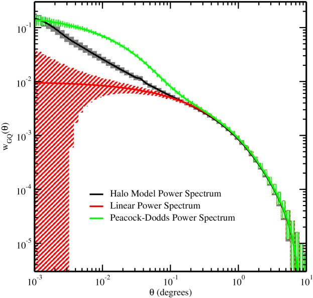
Note that background-foreground source correlation, equation (236), and the tangential shear-foreground galaxy correlation, equation (231), weigh the galaxy-mass cross-power spectrum with two different window functions involving a $J_{0}$ and a $J_{2}$, respectively. For a given projected distance $d_{A}\theta$, the two observational methods probe the galaxy-mass power spectrum at different scales. As shown in figure 46, the tangential shear-foreground galaxy correlation function probes the non-linear scales of the galaxy-mass correlation and, thus, more sensitive to the behavior of the single-halo contribution than the foreground-background correlation function of sources. The dependence of the non-linear scales in the shear-galaxy correlation suggests that it is more suitable to probe the physical aspects of how foreground galaxies trace their dark matter halos. On the other hand, the foreground-background source correlation function probes the clustering aspects of foreground sources that trace the linear density field.

In figure 47, we show the expected correlation between foreground galaxies in the Sloan Digital Sky Survey and background quasars at redshifts greater than 1. The expected errors suggest that the correlation will be measured out to angular scales of several degrees. Since sufficient statistics will soon be available, the catalog can be divided in to redshift bins and be combined with associated data on the shear-galaxy correlation for detailed studies on galaxy-mass cross clustering.

9 Halo applications to CMB: Secondary effects

The angular power spectrum of cosmic microwave background (CMB) temperature fluctuations is now a well known probe of cosmology. The anisotropies can be well described through linear physics involving Compton scattering and linearized general relativity. The well known features in the power spectrum, the acoustic oscillations at large angular scales and the damping tail at medium angular scales [214, 273, 261, 124], allow the ability to constrain most, or certain combinations of, parameters that define the currently favored CDM models with a cosmological constant [159, 141, 22, 297, 75]. This has led to a wide number of experimental attempts with results so far suggesting the evidence for acoustic peaks as expected in models with adiabatic initial conditions and a scale invariant power spectrum of fluctuations [187, 67, 107, 101].

The small angular scale temperature anisotropies contain a wide-variety of information related to the growth and evolution of large scale structure including non-linear aspects of clustering. Such a contribution from the low redshifts is partly contrary to the general assumption that CMB fluctuations are solely described by linear physics at the last scattering at a redshift $\sim$ 1100. There are two methods by which large scale structure of the local universe can modify CMB temperature: gravity and scattering. The gravitational contributions arise from variations in the frequency of CMB photons via gravitational redshifts and blueshifts [229, 222, 242, 52, 63, 165] and via deflection [26, 155, 169, 43, 230, 287, 89, 38, 243, 120] and time-delay [125] effects on CMB photons due to gravitational lensing. In the reionized epoch, with a population of free electrons, the CMB photons can also be Compton-scattered [206, 285, 144, 68, 72, 130, 123].

The large scale structure contributions to CMB, either due to gravity or scattering, can be modeled using the halo approach and their statistical properties can be calculated in detail, similar to the application of the halo models to galaxy and weak lensing statistics. Here, we will consider several such secondary contributions including the thermal and kinetic Sunyaev-Zel’dovich (SZ; [274]) effects, the gravitational lensing modification to CMB, and the non-linear contribution to the integrated Sachs-Wolfe effect (ISW; [229]) at small angular scales.

The anisotropy power spectrum at small angular scales has recently become the focus of several theoretical and experimental studies. Though there are several upper-limits and an initial detection of anisotropy power at small scales [66, 118, 271, 40], a wide-field CMB image is yet to be produced with resolution necessary for studies related to secondary effects. To this end, several experiments are now working towards obtaining such information either from direct imaging or interferometric techniques. These experimental attempts include the proposed 12 deg.² survey by [33] at the combined and expanded BIMA and OVRO arrays (CARMA), the Atacama Telescope (ACT; Lyman Page, private communication), and the BOLOCAM array on the Caltech Submillimeter Observatory (Andrew Lange, private communication). In the longer term, a few thousand sqr. degrees is proposed to be imaged in a few years with a wide-field bolometer array at the South Pole Telescope (John Carlstrom, private communication) and the Planck surveyor will allow detailed studies of certain secondary effects and foreground via multi-frequency all-sky maps.

9.1 The Thermal SZ effect

The SZ thermal effect arises from the inverse-Compton scattering of CMB photons by hot electrons along the line of sight. This effect has now been directly imaged towards massive galaxy clusters (e.g., [33, 140]), where temperature of the scattering medium can reach as high as 10 keV producing temperature changes in the CMB of order 1 mK at Rayleigh-Jeans wavelengths. The SZ effect is now well known for its main cosmological application involving measurements of the Hubble constant. The basic idea follows from the initial suggestions by Gunn [97] and Silk & White [262]: the SZ temperature decrement, $\Delta T\propto T_{e}n_{e}dl$, towards a given cluster can be combined with thermal Bremsstrahlung X-ray emission, $S_{x}\propto T_{e}^{1/2}n_{e}^{2}dl$, towards the same cluster to obtain an estimate of the line of sight distance through the cluster: $L\propto S_{x}/\Delta T^{2}$. This requires a measurement of $T_{e}(r)$ across the cluster; the isothermal assumption $T_{e}(r)=T_{0}$ is generally employed due to limitations on the observational front. A comparison of this distance to the projected separation of the cluster across the sky determines the angular diameter distance to the cluster, independent of cosmological distance ladder (see, [181, 182, 208, 94, 221, 127] for recent $H_{0}$ measurements). Through a cosmological model for the distance, one can extract parameters such as the Hubble constant and with measurements over a wide range in redshift, values for the matter density and the cosmological constant.

There are several limitations that prohibit a reliable measurement of the Hubble constant from the combined SZ and X-ray data, at least in the case of a single cluster. The usual spherical assumption for clusters are inconsistent with observations and can bias the distance measurement at the level of 10% to 20% [49, 272, 220]. The isothermal assumption for electron temperature has been shown to be inconsistent with numerically simulated galaxy cluster gas distributions, though, this assumption is yet to be tested with observations of galaxy clusters. In the case of clusters with significant cooling flows, it is clear that a single temperature cannot be used to describe the electron temperature; this again leads to biases at the few tens of percent level [228, 177]. Additional contributions at the 10% level and less include, the presence of contaminating radio point sources, either in the cluster [47] or background sources gravitationally lensed by the cluster potential [170], fluctuations in the background anisotropies lensed through the cluster [39] and the peculiar velocity contribution to the kinetic SZ effect. Though, in general, these effects limit the reliability of the Hubble constant measured towards a single cluster, a significant sample of clusters is expected to produce a measurement that is within the few percent level. In the case of projection effects involving ellipsoidal clusters, distributed following ellipticities observed for present-day cluster samples, it can be shown that for a sample of at least 25 or more clusters, the mean Hubble constant is consistent with the true value [49].

In the future when wide-field SZ surveys are available, we are more interested in the statistics of SZ effect, such as the SZ correlation function or power spectrum in real space. Since on top of the SZ effect, one also gets a contribution from the CMB anisotropy fluctuations, it is clear that one requires reliable ways to separate them and also contaminant foregrounds such as radio point sources and galactic dust. Due to the nature of inverse-Compton scattering, where photons are upscattered from low to high frequencies, the SZ effect, fortunately, bears a spectral signature that differs from other temperature fluctuations including the dominant CMB primary component (see, figure 48). In upcoming multifrequency CMB data, thus, the SZ contribution can be separated using its frequency dependence. This allows statistics related to the SZ effect be studied independently of, say, dominant CMB temperature fluctuations. As discussed in detail in [58], a multi-frequency approach can easily be applied to Planck surveyor missions (see, figure 49).

Figure 48: Frequency dependence of the SZ effect at a multipole of $l\sim 5000$. Here, we show the absolute value of temperature relative to the thermal CMB spectrum. For comparison, we also show the temperature fluctuations due to point sources (both radio at low frequencies and far-infrared sources at high frequencies; solid line), galactic synchrotron (long dashed line), galactic free-free (dotted line) and galactic dust (short dashed line). At small angular scales, frequencies around 50 to 100 GHz is ideal for a SZ experiment.

Figure 49: Recovery of the SZ signal with Planck multifrequency data: (a) A line of sight integrated model SZ map with the assumption that pressure traces dark matter with a scale independent bias at all scales, (b) The map smoothed at 20^′, (c) this SZ signal+noise from primary anisotropies and foregrounds, and (d) final recovered map with a SZ frequency spectrum. For Planck, the recovered spectrum is consistent with the input spectrum and allows a determination of the SZ power spectrum with a cumulative signal-to-noise greater than 100 [58].

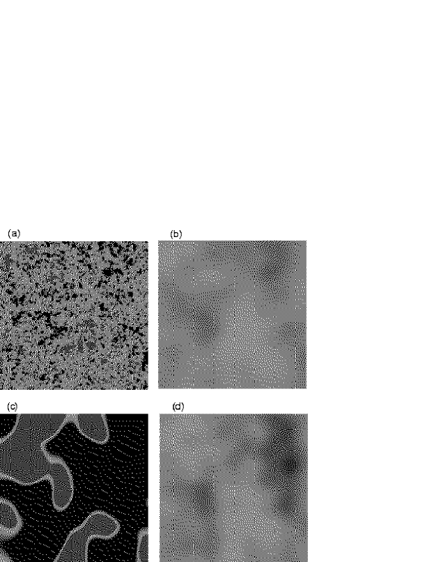
9.1.1 SZ Power Spectrum

The temperature decrement along the line of sight due to SZ effect can be written as the integral of pressure along the same line of sight

$$y\equiv\frac{\Delta T}{T_{\rm CMB}}=g(x)\int dra(r)\frac{k_{B}\sigma_{T}}{m_{e}c^{2}}n_{e}(r)T_{e}(r)\,$$ (238)

where $\sigma_{T}$ is the Thomson cross-section, $k_{B}$ is the Boltzmann’s constant, $n_{e}$ is the electron number density, $r$ is the comoving distance, and $g(x)=x{\rm coth}(x/2)-4$ with $x=h\nu/k_{B}T_{\rm CMB}$ is the spectral shape of the SZ effect. At Rayleigh-Jeans (RJ) part of the CMB, $g(x)=-2$. For the rest of this paper, we assume observations in the Rayleigh-Jeans regime of the spectrum, though, an experiment such as Planck with sensitivity beyond the peak of the spectrum can separate out these contributions based on the spectral signature, $g(x)$ [58] (see also, [277, 115] for frequency separation of CMB from foregrounds).

The SZ power spectrum, bispectrum and trispectrum are defined in the flat sky approximation in the usual way

$$\left<y({\mathbf{l}}_{1})y({\mathbf{l}}_{2})\right> = (2\pi)^{2}\delta_{\rm D}({\mathbf{l}}_{12})C_{l}^{\rm SZ}\,,$$

$$\left<y({\mathbf{l}}_{1})y({\mathbf{l}}_{2})y({\mathbf{l}}_{3})\right>_{c} = (2\pi)^{2}\delta_{\rm D}({\mathbf{l}}_{123})B^{\rm SZ}({\mathbf{l}}_{1},{\mathbf{l}}_{2},{\mathbf{l}}_{3})\,,$$

$$\left<y({\mathbf{l}}_{1})\ldots y({\mathbf{l}}_{4})\right>_{c} = (2\pi)^{2}\delta_{\rm D}({\mathbf{l}}_{1234})T^{\rm SZ}({\mathbf{l}}_{1},{\mathbf{l}}_{2},{\mathbf{l}}_{3},{\mathbf{l}}_{4})\,.$$ (239)

These can be written as a redshift projection of the pressure power spectrum, bispectrum and trispectrum, respectively:

$$C_{l}^{\rm SZ} = \int dr\frac{W^{\rm SZ}(r)^{2}}{d_{A}^{2}}P_{\Pi}\left(\frac{l}{d_{A}},r\right)\,,$$ (240)

$$B^{\rm SZ} = \int dr\frac{W^{\rm SZ}(r)^{3}}{d_{A}^{4}}B_{\Pi}\left(\frac{{\mathbf{l}}_{1}}{d_{A}},\frac{{\mathbf{l}}_{2}}{d_{A}},\frac{{\mathbf{l}}_{3}}{d_{A}},;r\right)\,,$$

$$T^{\rm SZ} = \int dr\frac{W^{\rm SZ}(r)^{4}}{d_{A}^{6}}T_{\Pi}\left(\frac{{\mathbf{l}}_{1}}{d_{A}},\frac{{\mathbf{l}}_{2}}{d_{A}},\frac{{\mathbf{l}}_{3}}{d_{A}},\frac{{\mathbf{l}}_{4}}{d_{A}},;r\right)\,.$$ (241)

Here, $d_{A}$ is the angular diameter distance. At RJ part of the frequency spectrum, the SZ weight function is

$$W^{\rm SZ}(r)=-2\frac{k_{B}\sigma_{T}\bar{n}_{e}}{a(r)^{2}m_{e}c^{2}}$$ (242)

where $\bar{n}_{e}$ is the mean electron density today. In deriving equation (241), we have used the Limber approximation [168] by setting $k=l/d_{A}$ and flat-sky approximation. Here, we have written the correlations in terms of the large scale structure pressure, denoted by $\Pi$, power spectrum, bispectrum and trispectrum.

The halo approach has been widely utilized to make analytical predictions on the statistics related to SZ thermal effect from the large scale structure such as the power spectrum (e.g., [44, 162]). Other approaches include a biased description of the pressure power spectrum with respect to the dark matter density field (e.g., [218, 58]). These analytical calculations are now fully complemented by numerical simulations (e.g., [61, 223, 246, 266]) which are now beginning to test the assumptions related to the halo based calculations. So far, comparisons between numerical simulations and the halo approach suggest significant agreement better than comparisons involving dark matter alone [224]. We will discuss reasons for this below.

First, we will describe the halo based approach to SZ statistics by introducing the clustering of large scale structure pressure. This is similar to the dark matter power spectrum and its projection along the line of sight that leads to weak lensing convergence power spectrum: the line of sight projections of the large scale structure pressure leads to the SZ effect.

9.1.2 Clustering Properties of Large Scale Structure Pressure

In order to describe the large scale structure pressure, we make use of the hydrostatic equilibrium between the gas and the dark matter distributions within halos. The hydrostatic assumption is supported by various observations of galaxy clusters, where the existence of regularity relations, such as the size-temperature relation [193], between physical properties of dark matter and baryon distributions suggest simple physical relations between the two properties.

Figure 50: The dark matter (NFW) profile and the ones predicted by the hydrostatic equilibrium for gas, as a function of the $b$ parameter (see equation 246) with $r_{s}=100$. The relative normalization between individual parameters is set using a gas fraction value of 0.1, though the NFW profile is arbitrarily normalized with $\rho_{s}=1$; the gas profiles scale with the same factor. For comparison, we also show a typical example of the so-called $\beta$ model $(1+r^{2}/r_{c}^{2})^{-3\beta/2}$ which is generally used as a fitting function for X-ray and SZ observations of clusters. We refer the reader to [179] and [275] for a detailed comparison of $\beta$ models and the NFW-gas profiles.

The hydrostatic equilibrium for gas with pressure $P$ and density $\rho_{g}$

$$\rho_{g}^{-1}\frac{dP}{dr}=-\frac{GM_{\delta}(r)}{r^{2}}\,$$ (243)

can be simplified in the limit gas is ideal, $P=\frac{k_{B}T_{e}}{\mu m_{p}}\rho_{g}$, and isothermal to obtain

$$\frac{k_{B}T_{e}}{\mu m_{p}}\frac{d\log\rho_{g}}{dr}=-\frac{GM_{\delta}(r)}{r^{2}}\,,$$ (244)

where $\mu=0.59$, corresponding to a hydrogen mass fraction of 76%. Here, now the $M_{\delta}(r)$ is the dark matter mass only out to a radius of $r$. Using a NFW profile for dark matter distribution, we can analytically calculate the baryon density profile $\rho_{g}(r)$

$$\rho_{g}(r)=\rho_{g0}e^{-b}\left(1+\frac{r}{r_{s}}\right)^{br_{s}/r}\,,$$ (245)

where $b$ is a constant, for a given mass [179, 275]:

$$b=\frac{4\pi G\mu m_{p}\rho_{s}r_{s}^{2}}{k_{B}T_{e}}\,.$$ (246)

The normalization, $\rho_{go}$, can be set to obtain a constant gas mass fraction for halos comparable with the universal baryon to dark matter ratio: $f_{g}\equiv M_{g}/M_{\delta}=\Omega_{b}/\Omega_{m}$. The total gas mass present in a dark matter halo within the virial radius, $r_{v}$, is

$$M_{g}(r_{v})=4\pi\rho_{g0}e^{-b}r_{s}^{3}\int_{0}^{c}dx\,x^{2}(1+x)^{b/x}\,.$$ (247)

The electron temperature can be calculated based on the virial theorem or similar arguments as discussed in [50]. Using the virial theorem, we can write

$$k_{B}T_{e}=\frac{\gamma G\mu m_{p}M_{\delta}}{3r_{v}}\,,$$ (248)

with $\gamma=3/2$. Since $r_{v}\propto M_{\delta}^{1/3}(1+z)^{-1}$ in physical coordinates, $T_{e}\propto M^{2/3}(1+z)$. The average density weighted temperature is

$$\left<T_{e}\right>_{\delta}=\int dM\,\frac{M}{\rho_{b}}\frac{dn}{dM}(M,z)T_{e}(M,z)\,.$$ (249)

In figure, we show the evolution of density weighted temperature from [224]. The results from numerical simulations are well reproduced with a Press-Schechter mass distribution for halos. For the $\Lambda$CDM cosmology, the halo model predicts a density weighted temperature for large scale structure electrons of $\sim$ 0.5 keV today; if halos out to a mass of $8\times 10^{14}$ M${}_{\hbox{$\odot$}}$ only included, this mean density weighted temperature decreases to 0.41 keV.

Figure 51: The variation in the density weighted temperature of electron as a function of redshift. The solid line shows the redshift evolution of the temperature in hydrodynamical simulations while the halo models, with varying halo masses, are shown in dotted and dashed lines. The figure is from [224].

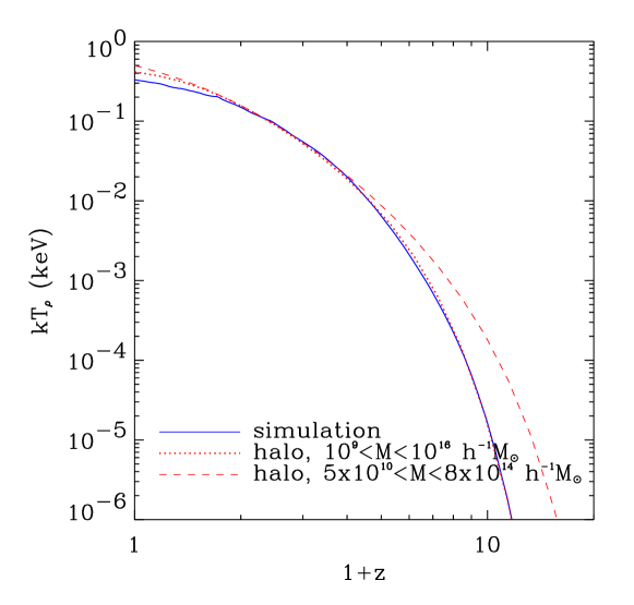
In figure 50, we show the NFW profile for the dark matter and arbitrarily normalized gas profiles predicted by the hydrostatic equilibrium and virial theorem for several values of $b$. As $b$ is decreased, such that the temperature is increased, the turn over radius of the gas distribution shifts to higher radii. As an example, we also show the so-called $\beta$ model that is commonly used to describe X-ray and SZ observations of galaxy clusters and for the derivation purpose of the Hubble constant by combined SZ/X-ray data. The $\beta$ model describes the underlying gas distribution predicted by the gas profile used here in equilibrium with the NFW profile, though, we find differences especially at the outer most radii of halos. This difference can be used as a way to establish the hydrostatic equilibrium of clusters, though, any difference of gas distribution at the outer radii should be accounted in the context of possible substructure and mergers.

A discussion on the comparison between the gas profile used here and the $\beta$ model is available in [179] and [275]. In addition, we refer the reader to [50] for full detailed discussion on issues related to modeling of pressure power spectrum using halo and associated systematic errors. Comparisons of the halo model predictions with numerical simulations are available in [246] and [224].

As discussed in [161], one can make several improvements to the above gas profile. One can constrain the gas distribution such that at outer most radii of halos, gas distributions follows that of the dark matter. This can be done by setting the slopes of dark matter and gas profiles to be the same beyond some radius. If gas is assumed to be in hydrostatic equilibrium, a gas profile that traces dark matter produces a temperature profile that varies with redshift. In general, one can obtain consistent solutions by assuming a polytropic form for pressure, $P\propto\rho_{g}T_{e}\propto\rho_{g}^{\gamma}$. As discussed in [161], predictions based on this prescription for cluster gas are more consistent with observations than the simple description involving an isothermal electron distribution

Figure 52: The (a) pressure and (b) pressure-dark matter cross power spectrum today broken into individual contributions under the halo description. For comparison, we also show the dark matter power spectrum under the halo model and in (a) pressure bias and in (b) pressure-dark matter correlation.

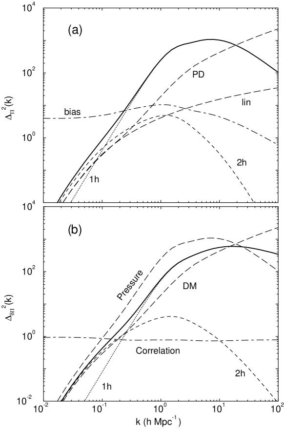
Given a description of the halo electron (or gas) profile and their temperature distribution, we can write the power spectrum of large scale structure pressure as

$$P_{\Pi}(k) = P^{1h}(k)+P^{2h}(k)\,,$$ (250)

$$P^{1h}(k) = M^{\Pi}_{02}(k,k)\,,$$ (251)

$$P^{2h}(k) = \left[M^{\Pi}_{11}(k)\right]^{2}P^{\rm lin}(k)\,,$$ (252)

where the two terms represent contributions from two points in a single halo (1h) and points in two different halos (2h) respectively.

Here, we redefine the integral in equation (4.2) for dark matter to account for pressure as

$$M^{\Pi}_{ij}(k_{1},\ldots,k_{j};z) \equiv \int dm\left(\frac{M}{\bar{\rho}}\right)^{j}\tilde{\frac{dn}{dm}}(m;z)b_{i}(m;z)T_{e}^{\j}(m;z)$$ (253)

$$\quad\quad\times[u_{\Pi}(k_{1}|m;z)\ldots u_{\Pi}(k_{j}|m;z)]\,,$$

with the three-dimensional Fourier transform of the gas profile substituted in equation (79) to obtain $u_{\Pi}(k|m;z)$. We define the bias and correlation of pressure, relative to dark matter, as

$${\rm bias}_{\Pi}(k)=\sqrt{\frac{P_{\Pi}(k)}{P_{\delta}(k)}}\,,$$ (254)

and

$$r_{ij}(k)=\frac{P_{\Pi-\delta}(k)}{\sqrt{P_{\Pi}(k)P_{\delta}(k)}}\,,$$ (255)

respectively. Here, $P_{\delta}$ is the dark matter power spectrum and $P_{\Pi-\delta}$ is the pressure-dark matter cross power spectrum. As presented for dark matter, we can similarly extend the derivation to calculate pressure bispectrum and trispectrum.

In figure 52(a), we show the logarithmic power spectrum of pressure and dark matter such that $\Delta^{2}(k)=k^{3}P(k)/2\pi^{2}$ with contributions broken down to the $1h$ and $2h$ terms today. As shown, the pressure power spectrum depicts an increase in power relative to the dark matter at scales out to few h Mpc^-1, and a decrease thereafter.

Figure 53: The baryon density (left) and temperature weighted density, or pressure (right), in a time-slice of a hydrodynamical simulation by [246]. As shown, most of the contribution to large scale structure pressure comes from massive halos while the baryon density is distributed over a wide range of mass scales and trace the filamentarity structures defined by the dark matter distribution. The figure is from U. Seljak based on simulations by [246].

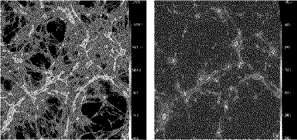
The decrease in power at small scales can be understood through the relative contribution to pressure as a function of the halo mass. In figure 54, we break the total dark matter power spectrum (a) and the total pressure power spectrum (b), to a function of mass. As shown, contributions to both dark matter and pressure comes from massive halos at large scales and by small mass halos at small scales. The pressure power spectrum is such that through temperature weighing, with $T_{e}\propto M^{2/3}$ dependence, the contribution from low mass halos to pressure is suppressed relative to that from the high mass end.

In figure 53, we show two images of a time slice through numerical simulations by [246]. The gas, or baryon, density distributions is such that it is highly filamentary and traces the large scale dark matter distribution. The pressure, however, is confined to virialized halos in the intersections between filaments. These are the massive clusters in the simulation box: the density weighted temperature, or pressure, of large scale structure is clearly dominant in massive clusters. Thus, the pressure power spectrum, at all scales of interest, can be easily described with halos of mass greater than $10^{14}$ $M_{\hbox{$\odot$}}$. A comparison of the dark matter and pressure power spectra, as a function of mass, in figure 54 reveals that the turn over in the pressure power spectrum results in an effective scale radius for halos with mass greater than $10^{14}$ M${}_{\hbox{$\odot$}}$. We refer the reader to [50] for further details on the pressure power spectrum and its properties.

Figure 54: The mass dependence on the dark matter power spectrum (a) and pressure power spectrum (b). Here, we show the total contribution broken in mass limits as written on the figure. As shown in (a), the large scale contribution to the dark matter power comes from massive halos while small mass halos contribute at small scales. For the pressure, in (b), only massive halos above a mass of $10^{14}$ M_sun contribute to the power.

Figure 55: The angular power spectra of SZ thermal and kinetic effects. As shown in (a), the thermal SZ effect is dominated by individual halos, and thus, by the single halo term, while the kinetic effect is dominated by the large scale structure correlations depicted by the 2-halo term. In (b), we show the mass dependence of the SZ thermal and kinetic effects with a maximum mass of $10^{16}$ and $10^{13}$ M${}_{\hbox{$\odot$}}$. The SZ thermal effect is strongly dependent on the maximum mass, while due to large scale correlations, kinetic effect is not.

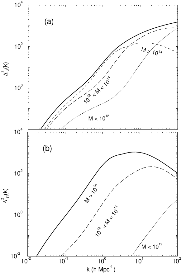
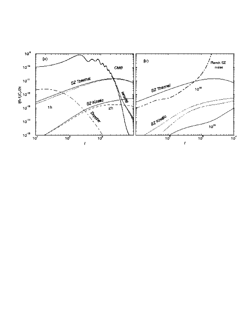
We can now use the pressure power spectrum to calculate the SZ angular power spectrum by projecting it along the line of sight following equation (241). In figure 55(a), we show the SZ power spectrum due to baryons present in virialized halos. As shown, most of the contributions to SZ power spectrum comes from individual massive halos, while the halo-halo correlations only contribute at a level of 10% at large angular scales. This is contrary to, say, the lensing convergence power spectrum, where most of the power at large angular scales is due to halo-halo correlations. The difference is effectively due to the dependence of pressure on most massive halos in the large scale structure and to a lesser, but somewhat related, reason that SZ weight function increases towards low redshifts. Note that the lensing weight function selectively probes the large scale dark matter density power spectrum at comoving distances half to that of background sources ($z\sim 0.2$ to 0.5 when sources are at a redshift of 1), but has no extra dependence on mass when compared to the SZ weight function.

Figure 56: The SZ power spectrum based on numerical simulations and the analytical calculations based on the halo model. The simulations are consistent with the mass distribution of halos in the simulated box. The decrease in power at largest scales is due to the lack of most massive halos, which are rare. The simulations are in good agreement with the halo based calculations. The figure is from [224].

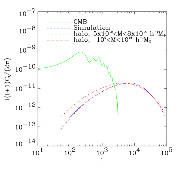
The predictions based on halo model are consistent with numerical simulations. In figure 56, we show the angular power spectrum of SZ effect as measured in numerical simulations by [224] and a comparison to the halo calculation following [50]. Note that simulations show a slight decrease in signal when the total mass included in the calculation is $10^{16}$ h^-1 M${}_{\hbox{$\odot$}}$. The measurements are best described with a halo mass distribution out to a maximum mass of $8\times 10^{14}$ h^-1 M${}_{\hbox{$\odot$}}$, consistent with the expectation that highest mass halos are rare and are not present in the simulated box.

Figure 57: Line of sight projected maps of the thermal (left) and kinetic (right) SZ effects. The maps are $1^{\circ}$ on a side and cover the same field of view. Note that the thermal SZ map picks out massive halos while contributions to kinetic SZ effect comes from wide range of masses. Unlike thermal SZ, which produces a negative decrement at Rayleigh-Jeans wavelengths, the kinetic SZ effect oscillates from negative and positive values depends on the direction of the velocity field. Here, structures in red are moving towards the observer while those in blue are moving away. This figure is from [266].

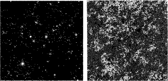
As we discuss later, the kinetic SZ effect has no such dependence on the massive halos and contributions to kinetic SZ effect comes from masses over a wide range. In figure 57, we show projected maps of the SZ thermal and SZ kinetic effect produced in simulations by [266]. The maps clearly show that the SZ thermal effect may be a useful way to map the massive structures in the universe.

The fact that the SZ power spectrum results mainly from the single halo term also results in a sharp reduction of power when the maximum mass used in the calculation is varied. For example, as discussed in [50] and illustrated in figure 55(b), with the maximum mass decreased from $10^{16}$ to $10^{13}$ M${}_{\hbox{$\odot$}}$, the SZ power spectrum reduced by a factor nearly two orders of magnitude in large scales and an order of magnitude at $l\sim 10^{4}$. The same dependence also suggests a significant sample variance for the SZ effect as massive halos are rare; as discussed in [51], the SZ statistics from small fields are likely to be heavily biased based on the mass distribution of halos. The same effect was found in numerical simulations where the power spectrum was observed to vary over a factor of $\sim$ 2 from 4 deg.² field to field over all scales probed [246]. For similar reasons, there is also a significant non-Gaussian contribution to the covariance of the SZ effect that may complicate the use of SZ power spectrum as a probe of cosmology or galaxy cluster physics [51].

Following [296], one can calculate the number counts of SZ halos under the approximation that gas traces dark matter and that the temperature of electrons can be related to velocity dispersion of the halo through virial arguments. This allows one to simplify the expected temperature decrement due to the SZ effect at RJ wavelengths

$$\frac{\Delta T}{T_{\rm CMB}}=-2\int dra(r)\frac{k_{B}\sigma_{T}}{m_{e}c^{2}}n_{e}(r)T_{e}(r)\approx-2\frac{\sigma_{T}}{m_{e}}\frac{\Omega_{b}}{\Omega_{m}}\int dr\frac{\sigma^{2}_{\rm dm}(r)}{2c^{2}}\rho_{\rm dm}(r)\,$$ (256)

where the temperature of electrons has been approximated via line of sight velocity dispersion of dark matter particles, $\sigma^{2}_{\rm dm}$.

Figure 58: Distribution of peak heights or number counts of thermal SZ temperature decrements in simulations (solid histograms) and in analytical calculations (solid curves). Dashed lines show the contributions to the total from halos with mass in the range $10^{13}-10^{14}$, $10^{14}-10^{15}$ and above $10^{15}$ from increasing temperature decrement values. Here $t_{\rm SZ}=\Delta T^{\rm SZ}/T_{\rm CMB}$. The figure is from [296].

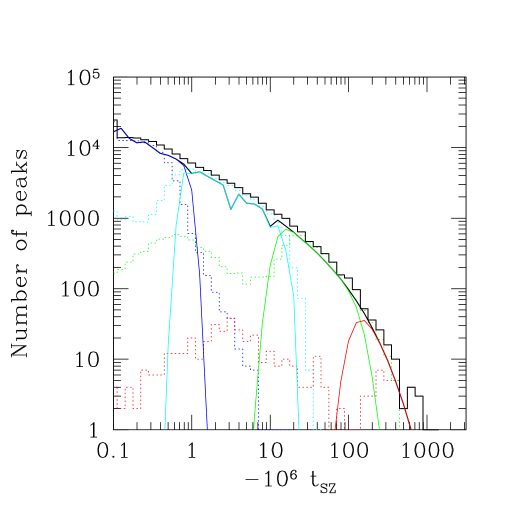
The expected number of peaks due to the thermal SZ effect can be evaluated by determining the expected SZ flux, integrated over the cluster, as a function of mass and then integrating over the mass function:

$$N({\rm SZ})=\int dmn(m)p(\Delta T^{\rm SZ}|m)d\Delta T^{\rm SZ}\,,$$ (257)

where the probability distribution of temperature fluctuations arises from the lognormal scatter in the concentration-mass relation [296]. Figure 58 shows that the counts predicted by this model are in good agreement with numerical simulations. Note, however, that the simulations were of dark matter only, so they also assumed that gas traces density. Hydrodynamical simulations have been used to test the extent to which gas traces dark matter; they show that gas pressure effects can be important at the low mass end. Therefore, one expects modifications to Figure 58 at the low mass end; counts based on hydrodynamical simulations can be found in e.g., [266, 61].

9.2 The kinetic SZ effect

Extending our calculation on the contribution of large scale structure gas distribution to CMB anisotropies through SZ effect, we can also study an associated effect involving baryons associated with halos in the large scale structure.

The bulk flow of electrons, that scatter CMB photons, lead to temperature fluctuations through the well known Doppler effect

$$T(\hat{\bf n})=\int drg(r)\hat{\bf n}\cdot{\bf v}(r\hat{\bf n},r)\,,$$ (258)

where ${\bf v}$ is the baryon velocity. In figure 55, we show the general Doppler effect due to the velocity field. The power spectrum is such that it peaks around the horizon at the scattering event projected on the sky today. On scales smaller than the horizon at scattering, the contributions are significantly canceled as photons scatter against the crests and troughs of the perturbation. As a result, the Doppler effect is moderately sensitive to how rapidly the universe reionizes since contributions from a sharp surface of reionization do not cancel [54]. Also important are the double scattering events, which first scatter out of the line of sight and the scatter back in, that do not necessarily cancel [144, 54].

The cancellations can be avoided by modulating the velocity field with electron number density fluctuations. This is the so-called Ostriker-Vishniac [206, 285] effect. The OV effect has been described as the contribution to temperature anisotropies due to baryon modulated Doppler effect in the linear regime of fluctuations. At non-linear scales, it is well known that the peculiar velocity of galaxy clusters, along the line of sight, also lead to a contribution to temperature anisotropies. This effect is commonly known as the kinetic Sunyaev-Zel’dovich effect and arises from the halo modulation of the Doppler effect associated with the velocity field [274]. The kinetic SZ effect can be considered as the OV effect extended to the non-linear regime of baryon fluctuations [119], however, it should be understood that the basic physical mechanism responsible for the two effects is the same and that there is no reason to describe them as separate contributions.

9.2.1 Kinetic SZ power spectrum

The kinetic SZ temperature fluctuations, denoted as ${\rm kSZ}$, can be written as a product of the line of sight velocity, under linear theory, and density fluctuations

$$T^{\rm kSZ}(\hat{\bf n})=\int drg(r)\hat{\bf n}\cdot{\bf v}_{g}(r,\hat{\bf n}r)\delta_{g}(r,\hat{\bf n}r)$$

$$\quad=-i\int drg\dot{G}G\int\frac{d^{3}{\bf k}}{(2\pi)^{3}}\int\frac{d^{3}{\bf k}^{\prime}}{(2\pi)^{3}}\delta_{\delta}^{\rm lin}({\bf k}-{\bf k}^{\prime})\delta_{g}({\bf k^{\prime}})e^{i{\bf k}\cdot\hat{\bf n}r}\left[\hat{\bf n}\cdot\frac{{\bf k}-{\bf k}^{\prime}}{|{\bf k}-{\bf k}^{\prime}|^{2}}\right]\,,$$

Here, we have used linear theory to write the large scale velocity field in terms of the linear dark matter density field. The multiplication between the velocity and density fields in real space has been converted to a convolution between the two fields in Fourier space. We can now expand the temperature perturbation due to the kinetic SZ effect, $T^{\rm kSZ}$, using spherical harmonics:

$$a_{lm}^{\rm kSZ} = -i\int d\hat{\bf n}\int dr\;(g\dot{G}G)\int\frac{d^{3}{\bf k_{1}}}{(2\pi)^{3}}\int\frac{d^{3}{\bf k_{2}}}{(2\pi)^{3}}\delta_{\delta}^{\rm lin}({\bf k_{1}})\delta_{g}({\bf k_{2}})$$ (260)

$$\times e^{i({\bf k_{1}+k_{2}})\cdot\hat{\bf n}r}\left[\frac{\hat{\bf n}\cdot{\bf k}_{1}}{k_{1}^{2}}\right]Y_{l}^{m\ast}(\hat{\bf n})\,,$$

where we have symmetrized by using ${\bf k}_{1}$ and ${\bf k}_{2}$ to represent ${\bf k}-{\bf k}^{\prime}$ and ${\bf k}^{\prime}$ respectively. Using

$$\hat{\bf n}\cdot{\bf k}=\sum_{m^{\prime}}\frac{4\pi}{3}kY_{1}^{m^{\prime}}(\hat{\bf n})Y_{1}^{m^{\prime}\ast}(\hat{{\bf k}})\,,$$ (261)

and the Rayleigh expansion (equation 175), we can further simplify and rewrite the multipole moments as

$$a_{lm}^{\rm kSZ}=-i\frac{(4\pi)^{3}}{3}\int dr\int\frac{d^{3}{\bf k}_{1}}{(2\pi)^{3}}\int\frac{d^{3}{\bf k}_{2}}{(2\pi)^{3}}\sum_{l_{1}m_{1}}\sum_{l_{2}m_{2}}\sum_{m^{\prime}}$$ (262)

$$\times(i)^{l_{1}+l_{2}}(g\dot{G}G)\frac{j_{l_{1}}(k_{1}r)}{k_{1}}j_{l_{2}}(k_{2}r)\delta_{\delta}^{\rm lin}({\bf k_{1}})\delta_{g}({\bf k_{2}})Y_{l_{1}}^{m_{1}}(\hat{{\bf k}}_{1})Y_{1}^{m^{\prime}}(\hat{{\bf k}}_{1})Y_{l_{2}}^{m_{2}}(\hat{{\bf k}}_{2})$$

$$\times \int d\hat{\bf n}Y_{l}^{m\ast}(\hat{\bf n})Y_{l_{1}}^{m_{1}\ast}(\hat{\bf n})Y_{l_{2}}^{m_{2}\ast}(\hat{\bf n})Y_{1}^{m^{\prime}\ast}(\hat{\bf n})\,.$$

We can construct the angular power spectrum by considering $\langle a_{l_{1}m_{1}}a^{*}_{l_{2}m_{2}}\rangle$. Under the assumption that the temperature field is statistically isotropic, the correlation is independent of $m$, and we can write the angular power spectrum as

$$\langle a_{l_{1}m_{1}}^{*,{\rm kSZ}}a_{l_{2}m_{2}}^{\rm kSZ}\rangle=\delta^{\rm D}_{l_{1}l_{2}}\delta^{\rm D}_{m_{1}m_{2}}C_{l_{1}}^{\rm kSZ}\,.$$ (263)

The correlation can be written using

$$\langle a^{\ast,{\rm kSZ}}_{l_{1}m_{1}}a^{\rm kSZ}_{l_{2}m_{2}}\rangle=\frac{(4\pi)^{6}}{9}\int dr_{1}g\dot{G}G\int dr_{2}g\dot{G}G$$ (264)

$$\times \int\frac{d^{3}{\bf k_{1}}}{(2\pi)^{3}}\frac{d^{3}{\bf k_{2}}}{(2\pi)^{3}}\frac{d^{3}{\bf k_{1}^{\prime}}}{(2\pi)^{3}}\frac{d^{3}{\bf k_{2}^{\prime}}}{(2\pi)^{3}}\langle\delta_{\delta}^{\rm lin}({\bf k_{1}^{\prime}})\delta_{g}({\bf k_{2}^{\prime}})\delta_{\delta}^{\ast{\rm lin}}({\bf k_{1}})\delta_{g}^{\ast}({\bf k_{2}})\rangle$$

$$\times \sum_{l_{1}^{\prime}m_{1}^{\prime}l_{1}^{\prime\prime}m_{1}^{\prime\prime}m_{1}^{\prime\prime\prime}l_{2}^{\prime}m_{2}^{\prime}l_{2}^{\prime\prime}m_{2}^{\prime\prime}m_{2}^{\prime\prime\prime}}(-i)^{l_{1}^{\prime}+l_{1}^{\prime\prime}}(i)^{l_{2}^{\prime}+l_{2}^{\prime\prime}}j_{l_{2}^{\prime}}(k_{1}^{\prime}r_{2})\frac{j_{l_{2}^{\prime\prime}}(k_{2}^{\prime}r_{2})}{k_{2}^{\prime}}\frac{j_{l_{1}^{\prime}}(k_{1}r_{1})}{k_{1}}j_{l_{1}^{\prime\prime}}(k_{2}r_{1})$$

$$\times \int d\hat{\bf m}Y_{l_{2}m_{2}}(\hat{\bf m})Y_{l_{2}^{\prime}m_{2}^{\prime}}^{\ast}(\hat{\bf m})Y_{l_{2}^{\prime\prime}m_{2}^{\prime\prime}}^{\ast}(\hat{\bf m})Y_{1m_{2}^{\prime\prime\prime}}^{\ast}(\hat{\bf m})$$

$$\times \int d\hat{\bf n}Y_{l_{1}m_{1}}^{\ast}(\hat{\bf n})Y_{l_{1}^{\prime}m_{1}^{\prime}}(\hat{\bf n})Y_{l_{1}^{\prime\prime}m_{1}^{\prime\prime}}(\hat{\bf n})Y_{1m_{1}^{\prime\prime\prime}}(\hat{\bf n})$$

$$\times \int d\hat{{\bf k}_{1}^{\prime}}\int d\hat{{\bf k}_{2}^{\prime}}Y_{l_{2}^{\prime}m_{2}^{\prime}}(\hat{{\bf k}_{1}^{\prime}})Y_{1m_{2}^{\prime\prime\prime}}(\hat{{\bf k}_{2}^{\prime}})Y_{l_{2}^{\prime\prime}m_{2}^{\prime\prime}}(\hat{{\bf k}_{1}^{\prime}})$$

$$\times \int d\hat{{\bf k}_{1}}\int d\hat{{\bf k}_{2}}Y_{l_{1}^{\prime}m_{1}^{\prime}}^{\ast}(\hat{{\bf k}_{1}})Y_{1m_{1}^{\prime\prime\prime}}^{\ast}(\hat{{\bf k}_{1}})Y_{l_{1}^{\prime\prime}m_{1}^{\prime\prime}}^{\ast}(\hat{{\bf k}_{2}})\,.$$

We can separate out the contributions such that the total is made of correlations following $\langle v_{g}v_{g}\rangle\langle\delta_{g}\delta_{g}\rangle$ and $\langle v_{g}\delta_{g}\rangle\langle v_{g}\delta_{g}\rangle$ depending on whether we consider cumulants by combining ${\bf k}_{1}$ with ${\bf k}_{1}^{\prime}$ or ${\bf k}_{2}^{\prime}$ respectively. After some straightforward but tedious algebra, and noting that

$$\sum_{m_{1}^{\prime}m_{2}^{\prime}}\left(\begin{array}[]{ccc}l_{1}^{\prime}&l_{2}^{\prime}&l_{1}\\ m_{1}^{\prime}&m_{2}^{\prime}&m_{1}\end{array}\right)\left(\begin{array}[]{ccc}l_{1}^{\prime}&l_{2}^{\prime}&l_{2}\\ m_{1}^{\prime}&m_{2}^{\prime}&m_{2}\end{array}\right)=\frac{\delta_{m_{1}m_{2}}\delta_{l_{1}l_{2}}}{2l_{1}+1}\,,$$ (265)

we can write

$$C_{l}^{\rm kSZ}=\frac{2^{2}}{\pi^{2}}\sum_{l_{1}l_{2}}\left[\frac{(2l_{1}+1)(2l_{2}+1)}{4\pi}\right]\left(\begin{array}[]{ccc}l&l_{1}&l_{2}\\ 0&0&0\end{array}\right)^{2}$$

$$\times \int dr_{1}g\dot{G}G\int dr_{2}g\dot{G}G\int k_{1}^{2}dk_{1}\int k_{2}^{2}dk_{2}$$

$$\times \Big{[}P_{\delta\delta}^{\rm lin}(k_{1})P_{gg}(k_{2})j_{l_{1}}(k_{2}r_{2})j_{l_{1}}(k_{2}r_{1})\frac{j_{l_{2}}^{\prime}(k_{1}r_{1})}{k_{1}}\frac{j_{l_{2}}^{\prime}(k_{1}r_{2})}{k_{1}}$$

$$+ P_{\delta b}(k_{1})P_{\delta b}(k_{2})j_{l_{2}}(k_{2}r_{1})\frac{j_{l_{1}}^{\prime}(k_{1}r_{1})}{k_{1}}j_{l_{1}}(k_{1}r_{2})\frac{j_{l_{2}}^{\prime}(k_{2}r_{2})}{k_{2}}\Big{]}\,.$$

Here, the first term represents the contribution from $\langle v_{g}v_{g}\rangle\langle\delta_{g}\delta_{g}\rangle$ while the second term is the $\langle v_{g}\delta_{g}\rangle\langle v_{g}\delta_{g}\rangle$ contribution, respectively. In simplifying the integrals involving spherical harmonics, we have made use of the properties of Clebsh-Gordon coefficients, in particular, those involving $l=1$. The integral involves two distances and two Fourier modes and is summed over the Wigner-3$j$ symbol to obtain the power spectrum. Since we are primary interested in the contribution at small angular scales here, we can ignore the contribution to the kSZ effect involving the correlation between linear density field and baryons and only consider the contribution that results from baryon-baryon and density-density correlations. In fact, under the halo description provided here, there is no correlation of the baryon field within halos and the velocity field traced by individual halos (see § 7). Thus, contribution to the baryon-velocity correlation only comes from the 2-halo term of the density field-baryon correlation. This correlation is suppressed at small scales and is not a significant contributor to the kinetic SZ power spectrum [119].

Similar to the Limber approximation [168], in order to simplify the calculation associated with $\langle v_{g}v_{g}\rangle\langle\delta_{g}\delta_{g}\rangle$, we use an equation involving completeness of spherical Bessel functions (equation 180) and apply it to the integral over $k_{2}$ to obtain

$$C_{l}^{\rm kSZ}=\frac{2}{\pi}\sum_{l_{1}l_{2}}\left[\frac{(2l_{1}+1)(2l_{2}+1)}{4\pi}\right]\left(\begin{array}[]{ccc}l&l_{1}&l_{2}\\ 0&0&0\end{array}\right)^{2}$$

$$\times \int dr_{1}\frac{(g\dot{G})^{2}}{d_{A}^{2}}\int k_{1}^{2}dk_{1}P_{\delta\delta}^{\rm lin}(k_{1})P_{gg}\left[\frac{l_{1}}{d_{A}};r_{1}\right]\left(\frac{j_{l_{2}}^{\prime}(k_{1}r_{1})}{k_{1}}\right)^{2}\,.$$

The alternative approach, which has been the calculational method in many of the previous papers [285, 72, 130, 68, 119], is to use the flat-sky approximation with the kinetic SZ power spectrum written as

$$C_{l}^{\rm kSZ}=\frac{1}{8\pi^{2}}\int dr\frac{(g\dot{G}G)^{2}}{d_{A}^{2}}P_{\delta\delta}(k)^{2}I_{v}\left(k=\frac{l}{d_{A}}\right)\,,$$ (274)

with the mode-coupling integral given by

$$I_{v}(k)=\int dk_{1}\int_{-1}^{+1}d\mu\frac{(1-\mu^{2})(1-2\mu y_{1})}{y_{2}^{2}}\frac{P_{\delta\delta}(ky_{1})}{P_{\delta\delta}(k)}\frac{P_{\delta\delta}(ky_{2})}{P_{\delta\delta}(k)}\,.$$

We refer the reader to [285] and [68] for details on this derivation. In above, $\mu=\hat{\bf k}\cdot\hat{\bf k_{1}}$, $y_{1}=k_{1}/k$ and $y_{2}=k_{2}/k=\sqrt{1-2\mu y_{1}+y_{1}^{2}}$. This flat-sky approximation makes use of the Limber approximation [168] to further simplify the calculation with the replacement of $k=l/d_{A}$. The power spectra here represent the baryon field power spectrum and the velocity field power spectrum; the former assumed to trace the dark matter density field while the latter is generally related to the linear dark matter density field through the use of linear theory arguments.

The correspondence between the flat-sky and all-sky formulation can be obtained by noting that in the small scale limit contributions to the flat-sky effect comes when $k_{2}=|{\bf k}-{\bf k}_{1}|\sim k$ such that $y_{1}\ll 1$. In this limit, the flat sky Ostriker-Vishniac effect reduces to a simple form given by [119]

$$C_{l}^{\rm kSZ}=\frac{1}{3}\int dr\frac{(g\dot{G}G)^{2}}{d_{A}^{2}}P_{gg}(k)v_{\it rms}^{2}\,.$$ (276)

Here, $v_{\it rms}^{2}$ is the rms of the uniform bulk velocity form large scales

$$v_{\it rms}^{2}=\int dk\frac{P_{\delta\delta}(k)}{2\pi^{2}}\,.$$ (277)

The $1/3$ arises from the fact that rms in each component is $1/3$rd of the total velocity. Similarly, one can reduce the all sky expression, equation (LABEL:eqn:redallsky), to that of the flat–sky, equation (276), in the small scale limit of $l\sim l_{1}\gg l_{2}$, with $l_{1}$ probing the density field [51].

Figure 59: The temperature fluctuation power $(\Delta T^{2}_{l}=l(l+1)/(2\pi)C_{l}T_{\rm CMB}^{2})$ for a variety of methods to calculate the kinetic SZ effect. Here, we show the contribution for a reionization redshift of $\sim$ 8 and an optical depth to reionization of 0.05. The contributions are calculated under the assumption that the baryon field traces the non-linear dark matter ($P_{g}(k)=P_{\delta}(k)$ with $P_{\delta}(k)$ predicted by the halo model), the linear density field ($P_{g}(k)=P^{\rm lin}(k)$), and the halo model for gas, with total and the 2-halo contributions shown separately. For the most part, the kinetic SZ effect can be described using linear theory, and the non-linearities only increase the temperature fluctuation power by a factor of a few at $l\sim 10^{5}$.

In figure 55, we show our prediction for the SZ kinetic effect and a comparison with the SZ thermal contribution. As shown, the SZ kinetic contribution is roughly an order of magnitude smaller than the thermal SZ contribution. There is also a more fundamental difference between the two: the SZ thermal effect, due to its dependence on highest temperature electrons is more dependent on the most massive halos in the universe, while the SZ kinetic effect arises more clearly due to large scale correlations of the halos that make the large scale structure.

The difference between the two effects arises from that fact that kinetic SZ effect is mainly due to the baryons and not the temperature weighted baryons that trace the pressure responsible for the thermal effect. Contributions to the SZ kinetic effect comes from baryons tracing all scales and down to small mass halos. The difference associated with mass dependence between the two effects suggests that a wide-field SZ thermal effect map and a wide-field SZ kinetic effect map will be different from each other in that massive halos, or clusters, will be clearly visible in a SZ thermal map while the large scale structure will be more evident in a SZ kinetic effect map. As shown with the thermal and kinetic SZ maps in figure 57 from [266], numerical simulations are in fact consistent with this picture (see, also [62]).

As shown in figure 55(b), the variations in maximum mass used in the calculation does not lead to orders of magnitude changes in the total kinetic SZ contribution, which is considerably less than the changes in the total thermal SZ contribution as a function of maximum mass. This again is consistent with our basic result that most contributions come from the large scale linear velocity modulated by baryons in halos. Consequently, while the thermal SZ effect is dominated by shot-noise contributions, and is heavily affected by the sample variance, the same is not true for the kinetic SZ effect.

In figure 59, we show several additional predictions for the kinetic SZ effect, following the discussion in [119]. Due to the density weighting, the kinetic SZ effect peaks at small scales: arcminutes for $\Lambda$CDM. For a fully ionized universe, contributions are moderately dependent on the optical depth $\tau$. Here, we assume an optical depth to ionization of 0.05, consistent with current upper limits on the reionization redshift from CMB [95] and other observational data (see, e.g., [100] and references therein). In figure 59, we have calculated the kinetic SZ power spectrum under several assumptions, including the case when gas is assumed to trace the non-linear density field and the linear density field. We compare predictions based on such assumptions to those calculated using the halo model. As shown, the halo model calculation shows slightly less power than when using the non-linear dark matter density field to describe clustering of baryons. This difference arises from the fact that baryons do not fully trace the dark matter in halos. Due to small differences, one can safely use the non-linear dark matter power spectrum to describe baryons. Using the linear theory only, however, leads to an underestimate of power by a factor of 3 to 4 at scales corresponding to multipoles of $l\sim 10^{4}$ to $10^{5}$ and may not provide an accurate description of the total kinetic SZ effect.

In addition to the contribution due to the line of sight motion of halos, there is an additional effect resulting from halo rotations as discussed by [53]. Here, the resulting rotational contribution to kinetic SZ effect was evaluated under the assumption that baryons in halos are corotating with dark matter; this assumption is primarily due to the lack of knowledge on angular momentum of gas in virialized halos from numerical simulations. In terms of the dark matter, recent high resolution numerical simulations show that the spatial distribution of angular momentum in dark matter halos has a universal profile (see e.g. [31, 286]). This profile is consistent with that of solid body rotation, but saturates at large values for angular momentum. The spatial distribution of angular momentum in most halos (80%) tend to be cylindrical and well-aligned with the spin of a halo. Also, angular momentum is almost independent with the mass of the halo and does not evolve with redshift except after major mergers.

For an individual cluster at a redshift $z$ with an angular diameter distance $d_{A}$, one can write the temperature fluctuation as an integral of the electron density, $n_{e}(r)$, weighted by the rotational velocity component, $\omega r\cos\alpha$, along the line of sight. Introducing the fact the line of sight velocity due to rotation is proportional to sine of the inclination angle of the rotational axis with respect to the observer, $i$, we write

$$\frac{\Delta T}{T}(\theta,\phi)=\sigma_{T}e^{-\tau}\eta(\theta)\cos\phi\sin i\,$$ (278)

where

$$\eta(\theta)=\int_{d_{c}\theta}^{R_{{\rm vir}}}\frac{2rdr}{\sqrt{r^{2}-d_{c}^{2}\theta^{2}}}n_{e}(r)\omega d_{c}\theta.$$ (279)

Here, $\theta$ is the line of sight angle relative to the cluster center and $\phi$ is an azimuthal angle measured relative to an axis perpendicular to the spin axis in the plane of the sky. In simplifying, we have introduced the fact that the angle between the rotational velocity and line of sight, $\alpha$, is such that $\alpha=\cos^{-1}d_{A}\theta/r$. In equation (279), $R_{\rm vir}$ is the cluster virial radius.

Figure 60: Contribution to temperature fluctuations through halo rotation for a cluster of mass $5\times 10^{14}$ M${}_{\hbox{$\odot$}}$ at a redshift of 0.5. The temperature fluctuations produce a distinct bipolar-like pattern on the sky with a maximum of $\sim$ 2.5 $\mu$K. Here, rotational axis is perpendicular to the line of sight and $x$ and $y$ coordinates are in terms of the scale radius of the cluster, based on the NFW profile.

To describe the halo rotations, we write the dimensionless spin parameter $\lambda(=J\sqrt{E}/GM^{5/2})$ following [31] as

$$\lambda=\frac{J}{2V_{c}M_{\rm vir}R_{\rm vir}}\frac{\sqrt{cg(c)}}{f(c)}\,$$ (280)

where the virial concentration for the NFW profile is $c=R_{\rm vir}/r_{s}$, $J$ is the total angular momentum, and $V_{c}^{2}=GM_{\rm vir}/R_{\rm vir}$. In Ref. [31], the probability distribution function for $\lambda$ was measured through numerical simulations and was found to be well described by a log normal distribution with a mean, $\bar{\lambda}$, of $0.042\pm 0.006$ and a width, $\sigma_{\lambda}$ of $0.50\pm 0.04$.

To relate angular velocity, $\omega$, to spin, we first integrate the NFW profile over a cluster to calculate $J$, and substitute in above to find

$$\omega=\frac{3\lambda V_{c}c^{2}f^{2}(c)}{R_{\rm vir}h(c)\sqrt{cg(c)}}\,.$$ (281)

The functions $f(c)$, $g(c)$ and $h(c)$, in terms of the concentration, follows as

$$f(c) = \ln(1+c)-\frac{c}{1+c}$$

$$g(c) = 1-\frac{2\ln(1+c)}{1+c}-\frac{1}{(1+c)^{2}}$$

$$h(c) = 3\ln(1+c)+\frac{c(c^{2}-3c-6)}{2(1+c)}\,.$$ (282)

In figure 60, we show the temperature fluctuation produced by the rotational component for a typical cluster with mass $5\times 10^{14}$ M${}_{\hbox{$\odot$}}$ at a redshift of 0.5. The maximal effect, with the mean spin parameter measured by [31], is on the order of $\sim$ 2.5 $\mu$K. The sharp drop towards the center of the cluster is due to the decrease in the rotational velocity. As shown, the effect leads to a distinct temperature distribution with a dipole like pattern across clusters. Here, we have taken the cluster rotational axis to be aligned perpendicular to the line of sight; as it is clear, when the axis is aligned along the line of sight, there is no resulting contribution to the SZ kinetic effect through scattering.

The order of magnitude of this rotational contribution can be understood by estimating the rotational velocity where the effect peaks. In equation (281), rotational velocity is $\omega\sim 3\lambda V_{c}/R_{\rm vir}$ with functions depending on the concentration in the order of a few ($\approx 2.4$ when $c=5$). Since the circular velocity for typical cluster is of order $\sim$ 1500 km s^-1, with $R_{\rm vir}\sim$ Mpc and $\bar{\lambda}\sim 0.04$, at typical inner radii of order $\sim 1/5R_{\rm vir}$, we find velocities of order $\sim$ 30 km s^-1. Since, on average, peculiar velocities for clusters are of order $\sim$ 250 km s^-1, the rotational velocity is lower by a factor of $\sim$ 8, when compared with the peculiar velocity of the typical cluster. Furthermore, since the kinetic SZ due to peculiar motion peaks in the center of the halo where the density is highest, while the rotational effect peaks away from the center, the difference between maximal peculiar kinetic SZ and rotational kinetic SZ temperature fluctuations is even greater. Note, however, each individual cluster has a different orientation and magnitude of peculiar velocity and rotation, thus the velocity-to-rotation ratio could vary a lot. In favorable cases where the peculiar velocity is aligned mostly across the line of sight, the rotational contribution may be important.

Figure 61: Temperature fluctuations due to galaxy clusters: (a) kinetic SZ effect involving peculiar motion, (b) lensing of CMB primary temperature fluctuations, and (c) the total contribution from kinetic SZ, lensing and rotational velocity. The total contribution leads asymmetric bipolar pattern with a sharp rise towards the center. We have not included the thermal SZ effect as its contribution can be separated from these effects, and primary temperature fluctuations, based on its frequency dependence. We use the same cluster as shown in figure 60.

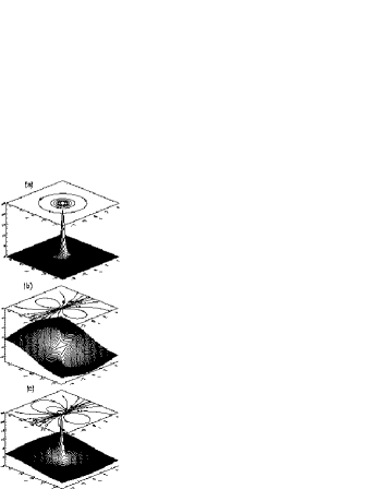
In figure 61, we show the kinetic SZ effect towards the same cluster due to the peculiar motion and the contribution resulting from the lensed CMB towards the same cluster. The latter contribution is sensitive to the gradient of the dark matter potential of the cluster along the large scale CMB gradient. In this illustration, we haven taken the CMB gradient to be the rms value with 13 $\mu$K arcmin^-1 following [247]. Previously, it was suggested that the lensed CMB contribution can be extracted based on its dipole like signature. Given the fact that the rotational contribution also leads to a similar pattern, any temperature distribution with a dipole pattern across a cluster cannot easily be prescribed to the lensing effect. However, as evident from figures 60 and 61, the dipole signature associated with the rotational scattering is limited to the inner region of the cluster while the lensing effect, due to its dependence on the gradient of the dark halo potential, covers a much larger extent. Also, the two dipoles need not lie in the same direction as the background gradient of the primary CMB fluctuations and the rotational axis of halos may be aligned differently. Thus, to separate the lensed effect and the rotational contribution from each other and from dominant kinetic SZ one can consider various filtering schemes (see, discussion in [247]). In figure 61, we have not included the dominant thermal SZ contribution since it can be separated from other contributions reliably if multifrequency data are available.

The interesting experimental possibility here is whether one can obtain a wide-field map of the SZ kinetic effect. Since it is now well known that the unique spectral dependence of the thermal SZ effect can be used to separate its contribution [58], it is likely that after such a separation, the SZ kinetic effect will be the dominant signal at small angular scales. To separate the SZ thermal effect, observations, at multifrequencies, are needed to arcminute scales. Upcoming interferometers and similar experiments will allow such studies to be eventually carried out. A wide-field kinetic SZ map of the large scale structure will allow an understating of the large scale velocity field of baryons, as the density fluctuations can be identified through cross-correlation of such a map with the thermal SZ map [51].

9.3 Non-Linear Integrated Sachs-Wolfe Effect

The integrated Sachs-Wolfe effect [229] results from the late time decay of gravitational potential fluctuations. The resulting temperature fluctuations in the CMB can be written as

$$T^{\rm ISW}(\hat{\bf n})=-2\int_{0}^{r_{0}}dr\dot{\Phi}(r,\hat{\bf n}r)\,,$$ (283)

where the overdot represent the derivative with respect to conformal distance (or equivalently look-back time). Writing multipole moments of the temperature fluctuation field $T(\hat{\bf n})$,

$$a_{lm}=\int d\hat{\bf n}T(\hat{\bf n})Y_{l}^{m}{}^{*}(\hat{\bf n})\,,$$ (284)

we can formulate the angular power spectrum as

$$\langle a_{l_{1}m_{1}}^{*}a_{l_{2}m_{2}}\rangle=\delta^{\rm D}_{l_{1}l_{2}}\delta^{\rm D}_{m_{1}m_{2}}C_{l_{1}}\,.$$ (285)

For the ISW effect, multipole moments are

$$a^{\rm ISW}_{lm} = i^{l}\int\frac{d^{3}{\bf k}}{2\pi^{2}}\int dr\dot{\Phi}({\bf k})I_{l}(k)Y_{l}^{m}(\hat{{\bf k}})\,,$$

with $I_{l}(k)=\int drW^{\rm ISW}(k,r)j_{l}(kr)$, and the window function for the ISW effect, $W^{\rm ISW}=-2$. The angular power spectrum is then given by

$$C_{l}^{\rm ISW}={2\over\pi}\int k^{2}dkP_{\dot{\Phi}\dot{\Phi}}(k)\left[I_{l}(k)\right]^{2}\,,$$ (287)

where the three-dimensional power spectrum of the time-evolving potential fluctuations are defined as

$$\langle\dot{\Phi}({\bf k_{1}})\dot{\Phi}({\bf k_{2}})\rangle=(2\pi)^{3}\delta_{D}({\bf k}_{1}+{\bf k}_{2})P_{\dot{\Phi}\dot{\Phi}}(k_{1})\,.$$ (288)

The above expression for the angular power spectrum can be evaluated efficiently under the Limber approximation [168] for sufficiently high $l$ values, usually in the order of few tens, as

$$C_{l}^{\rm ISW}=\int dr\frac{\left[W^{\rm ISW}\right]^{2}}{d_{A}^{2}}P_{\dot{\Phi}\dot{\Phi}}\left[k=\frac{l}{d_{A}},r\right]\,.$$ (289)

In order to calculate the power spectrum of time-derivative of potential fluctuations, we make use of the cosmological Poisson equation in equation (29) and write the derivative of the potential through a derivative of the density field and the scale factor $a$. Considering a flat universe with $\Omega_{K}=0$, we can write the full expression for the power spectrum of time-evolving potential fluctuations, as necessary for the ISW effect valid in all regimes of density fluctuations, as

$$P_{\dot{\Phi}\dot{\Phi}}(k,r) = {9\over 4}\left(\frac{\Omega_{m}}{a}\right)^{2}\left({H_{0}\over k}\right)^{4}$$ (290)

$$\quad\quad\times\left[\left(\frac{\dot{a}}{a}\right)^{2}P_{\delta\delta}(k,r)-2\frac{\dot{a}}{a}P_{\delta\dot{\delta}}(k,r)+P_{\dot{\delta}\dot{\delta}}(k,r)\right]\,.$$

To calculate the power spectrum involving the correlations between time derivatives of density fluctuations, $P_{\dot{\delta}\dot{\delta}}$, and the cross-correlation term involving the density and time-derivative of the density fields, $P_{\delta\dot{\delta}}$, we make use of the continuity equation in 19, which can be written in the form:

$$\dot{\delta}({\bf x},r)=-\nabla\cdot\left[1+\delta({\bf x},r)\right]{\bf v}({\bf x},r)\,.$$ (291)

In the linear regime of fluctuations, when $\delta({\bf x},r)=G(r)\delta({\bf x},0)\ll 1$, the time derivative is simply $\dot{\delta}^{\rm lin}({\bf x},r)=-\nabla\cdot{\bf v}({\bf x},r)$ leading to the well-known result for linear theory velocity field (equation 27). Thus, in linear theory, from equation (28), $P_{\dot{\delta}\dot{\delta}}\equiv k^{2}P_{vv}(k,r)=\dot{G}^{2}P_{\delta\delta}^{\rm lin}(k,0)$ and $P_{\delta\dot{\delta}}\equiv kP_{\delta v}(k,r)=G\dot{G}P_{\delta\delta}^{\rm lin}(k,0)$.

These lead to the well-known results for the linear ISW effect, with a power spectrum for $\dot{\Phi}$ as

$$P_{\dot{\Phi}\dot{\Phi}}^{\rm lin}(k,r)={9\over 4}\left(\frac{\Omega_{m}}{a}\right)^{2}\left({H_{0}\over k}\right)^{4}\left[-\frac{\dot{a}}{a}G(r)+\dot{G}\right]^{2}P_{\delta\delta}^{\rm lin}(k,0)\,.$$ (292)

The term within the square bracket is $\dot{F}^{2}$ where $F=G/a$ following derivation for the linear ISW effect in [54]. Even though, we have replaced the divergence of the velocity field with a time-derivative of the growth function, it should be understood that the contributions to the ISW effect comes from the divergence of the velocity field and not directly from the density field. Thus, to some extent, even the linear ISW effect reflects statistical properties of the large scale structure velocities.

In the mildly non-linear to fully non-linear regime of fluctuations, the approximation in equation (19), involving $\delta\ll 1$, is no longer valid and a full calculation of the time-derivative of density perturbations is required. This can be achieved in the second order perturbation theory, though, such an approximation need not be fully applicable as the second order perturbation theory fails to describe even the weakly non-linear regime of fluctuations exactly. Motivated by applications of the halo approach to large scale structure and results from numerical simulations [242, 174, 258], we consider a description for the time-derivative of density fluctuations and rewrite equation (19) as

$$\dot{\delta}({\bf x},r)=-\nabla\cdot{\bf v}({\bf x},r)-\nabla\cdot\delta({\bf x},r){\bf v}({\bf x},r)\,,$$ (293)

where we have separated the momentum term involving $p=(1+\delta)v$ to a velocity contribution and a density velocity product. In Fourier space, the power spectrum is simply $\dot{\delta}(k)=i{\bf k}\cdot p({\bf k})$ and the power spectrum of $\dot{\delta}$ can be calculated following the halo model description of the momentum-density field (§ 7.4).

Figure 62: The angular power spectrum of the full ISW effect, including non-linear contribution. The contribution called Rees-Sciama (RS) shows the non-linear extension, though for the total contribution, the cross term between the momentum field and the density field leads to a slight suppression between $l$ of 100 and 1000. The curve labeled “nl” is the full non-linear contribution while the curve labeled “lin” is the contribution resulting from the momentum field under the second order perturbation theory.

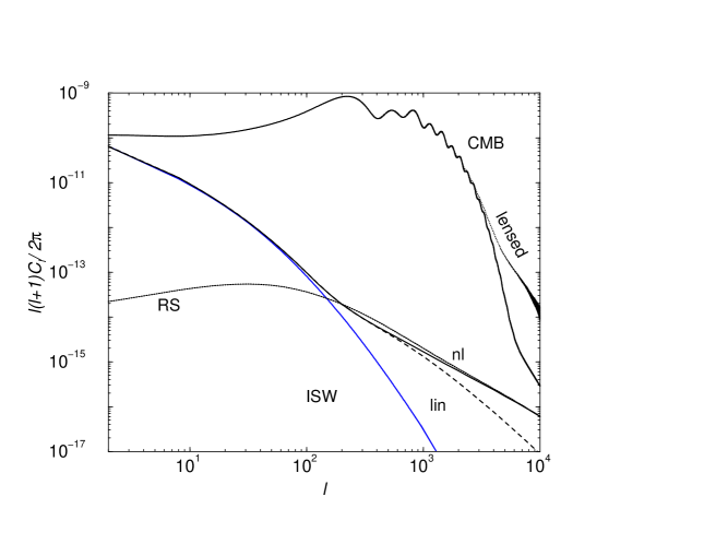
In addition to the power spectrum of density derivatives, in equation (290), we also require the cross power spectrum between density derivatives and density field itself $P_{\delta\dot{\delta}}$. In § 7.4, using the halo approach as a description of the momentum density field, we suggested that the cross-correlation between the density field and the momentum field can be well described as

$$P_{p\delta}(k)=\sqrt{P_{pp}(k)P_{\delta\delta}(k)}\,.$$ (294)

This is equivalent to the statement that the density and momentum density fields are perfectly correlated with a cross-correlation coefficient of 1; this relation is exact at mildly-linear scales while at deeply non-linear scales this perfect cross-correlation requires mass independent peculiar velocity for individual halos [258]. Using this observation, we make the assumption that $P_{\delta\dot{\delta}}\sim\sqrt{P_{\delta\delta}P_{\dot{\delta}\dot{\delta}}}$, which is generally reproduced under the halo model description of the cross-correlation between density field and density field derivatives. This cross-term leads to a 10% reduction of power at multipoles between 100 and 1000, when compared to the total when linear and non-linear contributions are simply added.

In figure 62, we show the angular power spectrum of the ISW effect with its non-linear extension (which we have labeled RS for Rees-Sciama effect [222]). The curve labeled ISW effect is the simple linear theory calculation with a power spectrum for potential derivatives given in equation (292). The curves labeled “lin” and “nl” shows the full non-linear calculation following the description given in equation (290) and using the linear theory or full non-linear power spectrum, in equation (154), for the density field, respectively. For the non-linear density field power spectrum, we use the halo approach for large scale structure clustering and calculate the power spectrum through a distribution of dark matter halos. We use linear theory to describe the velocity field in both linear and non-linear cases; since the velocity field only contributes as an overall normalization, through $v_{\rm rms}$, its non-linear effects, usually at high $k$ values, are not important due to the shape of the velocity power spectrum.

As shown in figure 62, the overall correction due to the non-linear ISW effect leads roughly two orders of magnitude increase in power at $l\sim 1000$. The difference between linear and non-linear theory density field power spectrum in equation (154), only leads to at most an order of magnitude change in power. Note that the curve labeled “lin” agrees with previous second order perturbation theory calculations of the Rees-Sciama effect [242], while the curve labeled “nl” is also consistent with previous estimates based on results from numerical simulations.

10 Summary

We have presented the halo approach to large scale structure clustering where we described the dark matter distribution of the local universe through a collection of collapsed and virialized halos. The statistical properties of the large scale structure can now be described through properties associated with these halos, such as their spatial distribution and the distribution of dark matter within these halos. These halo properties are well studied either through analytical models or numerical simulations and include such necessary information as the halo mass function, halo bias relative to linear density field and the halo dark matter profile.

The halo approach to clustering essentially allows one to bridge the linear regime described by perturbation theories to the non-linear regime described by clustering of dark matter within halos. The perturbation theories fail to describe the weakly to strongly non-linear regime completely, while, the halo model predictions are in better agreement with numerical results based on simulations. Though statistically averaged measurements are well produced by the halo based calculations, in detail, individual configurations of higher order correlations are only produced at the 20% level. The uncertainties here are mostly due to assumptions in the current halo model calculations, such as the use of spherical halos or ignoring the substructure within halos.

Though such uncertainties limit the accuracy of halo based calculations, the approach has the advantage that it can be easily extened to describe a wide variety of large scale structure properties. In this review, we have discussed stastical aspects involving the galaxy distribution, velocities and pressure. In order to calculation statistical aspects associated with these physical properties, we have introduced simple descriptions involving how they relate to dark matter within halos; almost all of these relations are based on numerical simulation results. Using these descriptions, we have discussed a wide number of applications of the halo model for non-linear clustering including observations of the dark matter distribution via weak lensing, galaxy properties via wide-field redshift and imaging surveys and applications to upcoming cosmic microwave background anisotropy experiments. The halo model has already become useful for several purposes, including (1) understand why the galaxy clustering essentially produces a power-law correlation function or a power spectrum, (2) estimate statistical biases in current and upcoming large scale structure weak lensing surveys, and (3) calculate the full covariance matrix associated with certain large scale structure observations, such as the angular correlation function of galaxies in the Sloan Digital Sky Survey, among others.

References

- [1] Appel, L., Jones, B.J.T. 1990, MNRAS, 245, 522.
- [2] Bacon, D., Refregier, A., Ellis R. 2000, MNRAS, 318, 625.
- [3] Bagla, J. S., 1998, MNRAS, 297, 251
- [4] Bardeen, J. M. 1980, PRD, 22 1882.
- [5] Bardeen, J. M., Steinhardt, P. J., Turner, M. S. 1983, Phys. Rev. D., 28 679.
- [6] Bardeen, J. M., Bond, J. R., Kaiser, N., Szalay, A. S. 1986, ApJ, 304, 15.
- [7] Bartelmann, M., Schneider, P. 2001, Physics Reports, 340 291.
- [8] Barkana, R. & Loeb, A. 2001, Physics Reports, 349, 125.
- [9] Benson, A. J., Cole, S., Frenk, C. S., Baugh, C. M., Lacey, C. G. 2000, MNRAS, 311, 793
- [10] Benson, A. J., Frenck, C. S., Baugh, C. M., Cole, S, Lacey, C. G. 2001, MNRAS, 327, 1041
- [11] Berlind, A. A., Weinberg, D. H. 2001, ApJ in press (astro-ph/0109001).
- [12] Bernardeau F., 1994, ApJ, 427, 51.
- [13] Bernardeau F., 1994, A&A, 291, 697.
- [14] Bernardeau, F., van Waerbeke, L., Mellier, Y. 1997, A&A, 322, 1.
- [15] Bernardeau, F., Colombi, S., Gaztañga, E., Scoccimarro, R. 2001, Physics Reports (in press).
- [16] Bertschinger, E. 1985, ApJS, 58, 1.
- [17] Birkinshaw, M. 1999, Physics Reports, 310, 97.
- [18] Blumenthal, G. R., Faber, S. M., Primack, J. R., Rees, M. J. 1984, Nature, 311, 517.
- [19] Bond J. R., Cole S., Efstathiou G., Kaiser N., 1991, ApJ, 379, 440.
- [20] Bond, J. R., Efstathiou, G. 1984, ApJ, 285, L45
- [21] Bond J. R., Myers S., 1996, ApJS, 103, 1.
- [22] Bond, J. R., Efstathiou, G., Tegmark, M., 1997, MNRAS, 291, L33.
- [23] Bower, R. J. 1991, MNRAS, 248, 332.
- [24] Bryan, G. L., Norman, M. 1998, ApJ, 495, 80.
- [25] Bryan, G. 2000, ApJ, 544, 1.
- [26] Blanchard, A., Schneider, J. 1987, A&A, 184, 1.
- [27] Blandford, R. D., Saust, A. B., Brainerd, T. G., Villumsen, J. V. 1991, MNRAS 251, 60.
- [28] Blasi, P., Sheth, R. K. 2000, Phys. Lett.B, 486, 233.
- [29] Bouchet, F. R., Juszkiewicz, R., Colombi, S. Pellat, R. 1992, ApJ, 394, L5.
- [30] Bullock, J. S., Kravtsov, A. V., Weinberg, D. H. 2000, ApJ, 539, 517
- [31] Bullock, J. S., Dekel, A., Kolatt, T. S. et al., 2001, ApJ, 555, 240
- [32] Bunn, E. F., White, M. 1997, ApJ, 480, 6.
- [33] Carlstrom, J. E., Joy, M., Grego, L. 1996, ApJ, 456, L75.
- [34] Carroll, S. M., Press, W. H., Turner, E. L. 1992, ARA&A, 30, 499.
- [35] Casas-Miranda, R., Mo, H., Sheth, R. K., Boerner, G. 2001, MNRAS in press (astro-ph/0105008).
- [36] Catelan, P., Lucchin, F., Matarrese, S., Porciani, C. 1998, MNRAS, 297, 692
- [37] Catelan, P., Kamionkowski, M., Blandford, R. D. 2001, MNRAS, 320, L7
- [38] Cayon, L., Martinze-Gonzalez, E., Sanz, J. 1993, ApJ, 413, 10.
- [39] Cen, R., 1998, ApJ, 498, L99.
- [40] Church, S. E., Ganga, K. M., Ade, P. A. R. et al. 1997, ApJ, 484, 523.
- [41] Colberg, J. M., White, S. D. M., Jenkins, A., Pearce, F. R. Yoshida 1999, MNRAS 308, 593.
- [42] Colberg, J. M., White, S. D. M., Yoshida, N. et al. 2000, MNRAS 319, 209.
- [43] Cole, S., Efstathiou, G. 1989, MNRAS, 239, 195.
- [44] Cole, S., Kaiser, N. 1988, MNRAS, 233, 637.
- [45] Cole, S., Kaiser, N., 1989, MNRAS, 237, 1127.
- [46] Connolly, A., Scranton, R., Johnstron, D. et al. 2001, ApJ submitted (astro-ph/0107417).
- [47] Cooray, A. R., Grego, L., Holzapfel, W. L., Joy, M., Carlstrom, J. E. 1998, AJ, 115, 1388.
- [48] Cooray, A. R. 1999, A&A, 348, 31.
- [49] Cooray, A. R. 2000, MNRAS, 313, 783
- [50] Cooray, A. 2000, Phys. Rev. D., 62, 103506.
- [51] Cooray, A. 2001, Phys. Rev. D., 64, 063514.
- [52] Cooray, A. 2002, Phys. Rev. D., 65, 083518.
- [53] Cooray, A., Chen, X. 2001, ApJ in press (astro-ph/0107544).
- [54] Cooray, A., Hu, W. 2000, ApJ, 534, 533.
- [55] Cooray, A., Hu, W. 2001, ApJ, 548, 7.
- [56] Cooray, A., Hu, W. 2001, ApJ, 554, 56.
- [57] Cooray, A., Hu, W. 2002, ApJ in press (astro-ph/0202411).
- [58] Cooray, A., Hu, W., Tegmark, M. 2000, ApJ, 544, 1.
- [59] Cooray, A., Hu, W., Miralda-Escudé, J. 2000b, ApJ, 536, L9.
- [60] Croft, R. A., & Metzler, C. 2000, 545, 561.
- [61] da Silva, A. C., Barbosa, D., Liddle, A. R., Thomas, P. A. 1999, MNRAS, 317, 37.
- [62] da Silva, A. C., Barbosa, D., Liddle, A. R., Thomas, P. A. 2001, MNRAS, 326, 155.
- [63] Dabrowski, Y., Hall, M. J., Sawicki, I.L, Lasenby, A. N. 2000, MNRAS, 318, 393.
- [64] Davis, M., Efstathiou, G., Frenk, C. S., White, S. D. M. 1992, Nature, 356, 489.
- [65] Davis, M., Miller, A., White, S. D. M. 1997, ApJ, 490, 63
- [66] Dawson, K. S., Holzapfel, W. L., Carlstrom, J. E., Joy, M., LaRoque, S. J., & Reese, E. D. 2001, ApJ, 553, L1.
- [67] de Bernardis, P., Ade, P. A. R., Bock, J. J. et al. 2000, Nature, 404, 955.
- [68] Dodelson, S. Jubas, J. M. 1995, ApJ, 439, 503.
- [69] Dodelson, S., Narayan, V. K., Tegmark, M. et al. 2001, AJ in press (astro-ph/0107421).
- [70] Dubinski, J., Carlberg, R. G. 1992, ApJ, 378, 496
- [71] Epstein, R. 1983, MNRAS, 205, 207.
- [72] Efstathiou, G. 1998, in Large Scale Motions in the Universe. A Vatican Study Week, ed. V. C. Rubin & G. V. Coyne (Princeton: Princeton University Press), 299.
- [73] Eisenstein, D. J., Hu, W. 1998, ApJ, 496, 605.
- [74] Eisenstein, D.J. & Hu, W. 1999, ApJ, 511, 5.
- [75] Eisenstein, D. J., Hu, W., Tegmark, M. 1999, ApJ, 518, 2.
- [76] Eisenstein, D. J. & Zaldarriaga, M. 2001, 546, 2.
- [77] Eke, V. R., Cole, S., Frenk, C. S. 1996, MNRAS, 282, 263
- [78] Eke, V. R., Navarro, J. F., Steinmetz, M. 2001, ApJ, 554, 114.
- [79] Engineer, S., Kanekar, N., Padmanabhan, T., 2000, MNRAS, 314, 279.
- [80] Evrard, A. E., MacFarland, T. J., Couchman, H. M. P. et al. 2002, ApJ in press (astro-ph/0110246)
- [81] Ferreira, P.G., Magueijo, J. & Gorksi, K.M. 1998, ApJ, 503, 1.
- [82] Fillmore, J., Goldreich, P. 1984, ApJ, 281, 9.
- [83] Fischer, P., Mckay, T. A., Sheldon, E. et al. 2000, AJ, 120, 1198.
- [84] Fosalba, P., Gaztañaga, E., 1998, MNRAS, 301, 535.
- [85] Fry, J. N., Seldner, M. 1982, ApJ, 259, 474.
- [86] Fry, J. N. 1984, ApJ, 279, 499.
- [87] Fry, J. N. 1996, ApJ, 461, L65.
- [88] Fry, J., Gaztañaga, E., 1993, ApJ, 413, 447
- [89] Fukugita, M., Futumase, T., Kasai, M., Turner, E. L. 1992, ApJ, 393, 3.
- [90] Gangui, A., Lucchin, F., Matarrese, S. & Mollerach, S. 1994, ApJ, 430, 447.
- [91] Gaztañaga, E., Fosalba, P., 1998, MNRAS, 301, 524.
- [92] Ghigna, S., Moore, B., Governato, F., Lake, G., Quinn, T., Stadel, J. 2000, ApJ, 544, 616.
- [93] Goroff, M. H., Grinstein, B., Rey, S.-J., Wise, M. 1986, ApJ, 311, 6.
- [94] Grego, L., Carlstrom, J. E., Joy, M. K. et al. 2000, ApJ, 539, 39.
- [95] Griffiths, L. M., Barbosa, D., Liddle, A. R. 1999, MNRAS, 308, 845.
- [96] Gunn, J. E., Gott, J. R. III, 1972, ApJ, 176, 1.
- [97] Gunn, J. E. 1978, In Observational Cosmology, I. eds. A. Maeder, L. Martinet, G. Tammann. Sauverny: Geneva Observatory
- [98] Guth, A. H., Pi, S.-Y. 1982, Phys. Rev. Lett., 49, 1110.
- [99] Guzik, J. & Seljak, U. 2001, 321, 439.
- [100] Haiman, Z., & Knox, L. 1999, in Microwave Foregrounds, ed. A. de Oliveira-Costa & M. Tegmark (ASP: San Fransisco).
- [101] Halverson, N. W., Leitch, E. M., Pryke, C. et al. 2002, ApJ. 568, 38.
- [102] Hamilton, A. J. S., Kumar, P., Lu, E., Matthews, A. 1991, ApJ, 374, L1.
- [103] Hamilton, A. J. S. 1997, MNRAS, 289, 285.
- [104] Hamilton, A. J. S. 2000, MNRAS, 312, 257.
- [105] Hamilton, A. J. S. & Tegmark, M. 2000, MNRAS, 312, 285.
- [106] Hanami, H., 2001, MNRAS, 327, 721.
- [107] Hanany, S., Ade, P., Balbi, A. et al. 2000, ApJ, 545, L5.
- [108] Harrison, E. 1970, Phys. Rev. D., 1, 2726.
- [109] Hawkings, S. W. 1982, Phys. Lett. B., 115, 295.
- [110] Heavens, A., Refregier, A., Heymans, C. 2000, MNRAS, 319, 649.
- [111] Hernquist, L., 1990, ApJ, 356, 359.
- [112] Henry, J. P. 2000, ApJ, 534, 565.
- [113] Hinshaw, G., Banday, A.J., Bennett, C.L., Gorski, K.M., & Kogut, A 1995, ApJ, 446, 67.
- [114] Hivon, E., Bouchet, F. R., Colombi, S., Juszkiewicz, R., 1995 A&A, 298, 643.
- [115] Hobson, M. P., Jones, A. W., Lasenby, A. N., Bouchet, F. R. 1998, MNRAS, 299, 895.
- [116] Hoffman, Y., Shaham, J. 1985, ApJ, 297, 16.
- [117] Holtzman, J. A. 1989, ApJS, 71, 1.
- [118] Holzapfel, W. L., Carlstrom, J. E., Grego, L., Joy, M., Reese, E.D. 2000, ApJ, 539, 57.
- [119] Hu, W. 2000a, ApJ, 529, 12.
- [120] Hu, W. 2000b, Phys. Rev. D., 62, 043007.
- [121] Hu W., Tegmark M. 1999, ApJ, 514, L65.
- [122] Hu, W. & White M. 1996, A&A, 315, 33.
- [123] Hu, W., Scott, D., Sugiyama, N., White, M. 1995, Phys. Rev. D., 52, 5498.
- [124] Hu, W., Sugiyama, N., Silk, J. 1997, Nature, 386, 37.
- [125] Hu, W., Cooray, A. 2001, Phys. Rev. D., 63, 023504.
- [126] Hu W., White M. 2001, ApJ, 554, 67.
- [127] Hughes, J. P., Birkinshaw, M. 1998, ApJ, 501, 1.
- [128] Hui, L. 1999, ApJ, 519, L9.
- [129] Icke V., 1973, A& A, 27, 1
- [130] Jaffe, A. H., Kamionkowski, M. 1998, Phys. Rev. D., 58, 043001.
- [131] Jain, B., Mo H.J., White, S.D.M. 1995, MNRAS, 276, 25.
- [132] Jain, B., Bertschinger, E. 1996, ApJ, 456, 43.
- [133] Jain B., Seljak U. 1997, ApJ, 484, 560
- [134] Jain, B., Seljak, U. & White, S. D. M. 2000, ApJ, 530, 547.
- [135] Jenkins A., Frenk C. S., White S. D. M., Colberg J. M., Cole S., Evrard A. E., Couchman H. M. P., Yoshida N., 2001, MNRAS, 321, 372.
- [136] Jetzer, Ph., Koch, P., Piffaretti, R., Puy, D., Schindler, S. 2002,astro-ph/0201421
- [137] Jing, Y. P., Mo, H. J., Boerner, G. 1998, ApJ, 494, 1.
- [138] Jing, Y. P. 2000, ApJ, 535, 30.
- [139] Jing, Y. P, & Suto, Y. 2002, ApJ, in press.
- [140] Jones, M. Saunders, R., Alexander, P., et al. 1993, Nature, 365, 320.
- [141] Jungman, G., Kamionkowski, M., Kosowsky, A., Spergel, D. N., 1995, Phys. Rev. D., 54, 1332.
- [142] Juszkiewicz, R., Springel, V., Durrer, R. 1999, ApJ, 518, L25.
- [143] Kaiser, N. 1984, ApJ, 284, 9.
- [144] Kaiser, N. 1984, ApJ, 282, 374.
- [145] Kaiser, N. 1987, MNRAS, 227, 1.
- [146] Kaiser, N. 1992, ApJ, 388, 286.
- [147] Kaiser, N. 1998, ApJ, 498, 26.
- [148] Kaiser, N. , Squires, G. 1993, ApJ, 404, 411.
- [149] Kaiser, N. , Squires, G., Fahlman, G., Woods, D. 1994, in ”Clusters of galaxies, eds. F. Durret, A. Mazure & J. Tran Thanh Van, Editions Frontieres.
- [150] Kaiser, N. , Squires, G., Broadhurst, T. 1995, ApJ, 449, 460.
- [151] Kamionkowski, M., Kosowsky, A., Stebbins, A. 1997a, PRD, 55, 7368
- [152] Kamionkowski, M., Babul, A., Cress, C. M., Refregier, A. 1998, MNRAS, 301, 1064.
- [153] Kamionkowski, M., Buchalter, A. 1999, ApJ, 514, 7.
- [154] Kamionkowski, M., Kosowsky, A., 1999, Ann.Rev.Nucl.Part.Sci., 49, 77.
- [155] Kashlinsky, A. 1988, ApJ, 331, L1.
- [156] Kauffmann, G., White, S. D. M., Guiderdoni, B. 1993, MNRAS, 264, 201.
- [157] Kauffmann, G., Colberg, J. M., Diaferio, A., White, S. D. M. 1999, MNRAS, 303, 188
- [158] Klypin, A., Gottlöber, S., Kravtsov, A. V., Khokhlov, A. M. 1999, ApJ, 516, 530.
- [159] Knox, L. 1995, Phys. Rev. D., 52, 4307.
- [160] Kolb, E. W., Turner, M. S. 1990, The Early Universe (Addison-Wesley).
- [161] Komatsu, E., Seljak, U. 2001, MNRAS, 327, 1353.
- [162] Komatsu, E. Kitayama, T., 1999, ApJ, 526, L1.
- [163] Lacey, C., Cole, S. 1993, MNRAS, 262, 627.
- [164] Lahav, O., Lilje, P. B., Primack, J. R., Rees, M. J. 1991, MNRAS, 251, 128.
- [165] Lasenby, A. N., Doran, C. J. L., Hobson, M. P., Dabrowski, Y., Challinor, A. D. 1999, MNRAS, 302, L748.
- [166] Lee J., Shandarin S., 1998, ApJ, 500, 14.
- [167] Lightman, A. P., Schechter, P. L. 1990, ApJS, 74, 831.
- [168] Limber, D. 1954, ApJ, 119, 655.
- [169] Linder, E. V., 1988, A&A, 206, 1999.
- [170] Loeb, A., Refregier, A. 1997, ApJ, 476, 59.
- [171] Ma, C.-P., Caldwell, R. R., Bode, P. & Wang, L. 1999, ApJ, 521, L1.
- [172] Ma, C.-P., Fry, J. N. 2000b, ApJ, 543, 503.
- [173] Ma, C.-P., Fry, J. N. 2000c, ApJ, 538, L107.
- [174] Ma, C.-P., Fry, J. N. 2002, PRL, 88, 211301.
- [175] Mackey, J., White, M., Kamionkowski, M. 2002, MNRAS, 332, 788.
- [176] Maddox, S. J., Efstathiou, G., Sutherland, W. J. Loveday, L. 1990, MNRAS, 242, 43.
- [177] Majumdar, S., Nath, B. P. 2000, ApJ, 542, 597.
- [178] Makino, N., Sasaki, S., Suto, Y. 1992, Phys. Rev. D., 46, 585.
- [179] Makino, N., Sasaki, S., Suto, Y. 1998, ApJ, 497, 555.
- [180] Manrique, A., Salvador-Solé, E., 1995, ApJ, 453, 6.
- [181] Mason, B. S., Myers, S. T., Readhead, A. C. S. 2001, ApJ, 555, L11.
- [182] Mauskopf, P. D., Ade, P. A. R., Allen, S. W., et al. 2000, ApJ, 538, 505.
- [183] McClelland, J. & Silk, J. 1977b, ApJ, 217, 331.
- [184] McClelland, J. & Silk, J. 1978, ApJS, 36, 389.
- [185] Meiksin, A. & White, M. 1999, MNRAS, 308, 1179.
- [186] Mellier, Y. 1999, Ann. Rev. Astro. Astrop. 37, 127.
- [187] Miller, A. D., Caldwell, R., Devlin, M. J. et al. 1999, ApJ, 524, L1.
- [188] Miralda-Escudé J. 1991, ApJ, 380, 1.
- [189] Mo, H. J., Jing, Y. P., White, S. D. M. 1997, MNRAS, 284, 189.
- [190] Mo, H. J., White, S. D. M. 1996, MNRAS, 282, 347.
- [191] Moessner, R., & Jain, B. 1998, MNRAS, 294, L18.
- [192] Moessner, R., Jain, B., Villumsen, J. V. 1998, MNRAS, 294, 291.
- [193] Mohr, J. J. Evrard, A. E. 1997, ApJ, 491, 38.
- [194] Monaco, P. 1995, ApJ, 447, 23.
- [195] Moore, B., Quinn, T., Governato, F., Stadel, J., & Lake, G. 1999, MNRAS, 310, 1147.
- [196] Munshi, D. & Jain, B. 2000, MNRAS, 318, 109.
- [197] Nakamura, T. T., Suto, Y. 1997, Prog. in Theor. Phys. 97, 49.
- [198] Navarro, J., Frenk, C., White, S. D. M., 1996, ApJ, 462, 563.
- [199] Neyman, J. & Scott, E. L. 1952, ApJ, 116, 144.
- [200] Neyman, J., Scott, E. L. & Shane, C. D. 1953, ApJ, 117, 92.
- [201] Neyman, J., Scott, E. L. & Shane, C. D. 1954, ApJS, 1, 269.
- [202] Nityananda, R., Padmanabhan, T. 1994, MNRAS, 271, 976.
- [203] Norberg, P., Baugh, C. M., Hawkins, E. et al. 2001, MNRAS, 328, 64.
- [204] Nusser, A. & Dekel, A. 1993, ApJ, 405, 437.
- [205] Nusser, A. & Sheth, R. K. 1999, MNRAS, 303, 685.
- [206] Ostriker, J.P., & Vishniac, E.T. 1986, ApJ, 305, L51.
- [207] Outram, P. J., Hoyle, F., Shanks, T., Boyle, B. J., Croom, S. M., Loaring, N. S., Miller, L., Smith, R. J. 2001, MNRAS, 328, 174.
- [208] Patel, S. K., Joy, M., Carlstrom, J. E. et al. 2000, ApJ, 541, 37.
- [209] Peacock, J.A., Dodds, S.J. 1994, MNRAS, 267, 1020.
- [210] Peacock, J.A., Dodds, S.J. 1996, MNRAS, 280, L19.
- [211] Peacock, J. A., & Heavens, A. F., 1990, MNRAS, 243, 133.
- [212] Peacock, J. A., Smith, R. E. 2000, MNRAS, 318, 1144.
- [213] Peacock, J. A., Cole, S., Norberg, P., et al. 2001, Nature, 410, 169.
- [214] Peebles, P. J. E., Yu, J. T., 1970, ApJ, 162, 815.
- [215] Peebles, P. J. E. 1974, ApJ, 189, L51.
- [216] Peebles, P. J. E. 1980, The Large-Scale Structure of the Universe, (Princeton: Princeton Univ. Press).
- [217] Peebles, P. J. E. 1980, ApJ, 263, L1.
- [218] Persi, F. M., Spergel, D. N., Cen, R., Ostriker, J. P. 1995, ApJ, 442, 1.
- [219] Press, W. H., Schechter, P. 1974, ApJ, 187, 425.
- [220] Puy, D., Grenacher, J., Jetzer, Ph., Signore, M. 2000, A&A, 363, 415.
- [221] Reese, E. D., Mohr, J. J., Carlstrom, J. E. et al. 2000, ApJ, 533, 38.
- [222] Rees, M. J. & Sciama, D. N. 1968, Nature, 519, 611.
- [223] Refregier, A., Komatsu, E., Spergel, D. N., Pen, U.-L. 1999, Phys. Rev. D., 61, 123001.
- [224] Refregier, A., Teyssier, R. 2001, Phys. Rev. D. submitted, astro-ph/0012086.
- [225] Refregier, A., 2001, MNRAS submitted, astro-ph/0105178.
- [226] Refregier, A., Bacon, D. 2001, MNRAS submitted, astro-ph/0105179.
- [227] Rice S. 0., 1954, in Selected papers on noise and stochastic processes, ed. Wax, N., Dover, N.Y.
- [228] Roettiger, K., Stone, J. M., Mushotzky, R. F. 1997, ApJ, 482, 588.
- [229] Sachs, R. K., & Wolfe, A. M., 1967, ApJ, 147, 73.
- [230] Sasaki, M., 1989, MNRAS, 240, 415.
- [231] Saslaw, W. C., Chitrem S. M., Itoh, M., Inagaki, S. 1990, ApJ, 365, 419
- [232] Scherrer, R.J., Bertschinger, E. 1991, ApJ, 381, 349.
- [233] Schneider P. 1996, ApJ, MNRAS, 283, 837.
- [234] Schneider P., van Waerbeke, L., Jain, B., Guido, K. 1998, MNRAS, 296, 873.
- [235] Scoccimarro, R., Zaldarriaga, M. & Hui, L. 1999, ApJ, 527, 1.
- [236] Scoccimarro, R., Sheth, R., Hui, L. & Jain, B. 2001, ApJ, 546, 20.
- [237] Scoccimarro, R., Sheth, R. K. 2002, 329, 629.
- [238] Scoccimarro, R. & Frieman, J. 1999, ApJ, 520, 35.
- [239] Scoccimarro, R., Couchman, H. M. P. 2001, MNRAS, 325, 1312.
- [240] Scranton, R. 2002, MNRAS, 332, 697.
- [241] Scranton, R., Johnston, D., Dodelson, S. et al. 2001, AJ in press (astro-ph/0107416).
- [242] Seljak, U. 1996a, ApJ, 460, 549.
- [243] Seljak, U. 1996b, ApJ, 463, 1.
- [244] Seljak, U. 2000, MNRAS, 318, 203.
- [245] Seljak, U. 2001, MNRAS, 325, 1359.
- [246] Seljak, U, Burwell, J., Pen, U.-L. 2001, Phys. Rev. D., 63, 063001.
- [247] Seljak, U., Zaldarriaga, M. 2000, ApJ, 538, 57.
- [248] Sheldon, E., Annis, J., Bohringer, H. et al. 2001 ApJ, 554, 881.
- [249] Sheth, R. K. 1996, MNRAS, 279, 1310.
- [250] Sheth, R. K., & Jain, B. 1997, MNRAS, 285, 231.
- [251] Sheth, R. K., & Jain, B. 2002, MNRAS, submitted
- [252] Sheth, R. K., & Lemson, G. 1999, MNRAS, 304, 767.
- [253] Sheth, R. K., Diaferio, A. 2001, MNRAS, 322, 901
- [254] Sheth, R. K., & Tormen, G. 1999, MNRAS, 308, 119.
- [255] Sheth, R. K., & Tormen, G. 2001, MNRAS, 323, 1.
- [256] Sheth, R. K., & Tormen, G. 2002, MNRAS, 329, 61.
- [257] Sheth, R. K., Mo, H., Tormen, G., 2001, MNRAS 323, 1
- [258] Sheth, R. K., Diaferio, A., Zehavi, I. 2001, MNRAS submitted.
- [259] Sheth, R. K., Hui, L., Diaferio, A., Scoccimarro, R. 2001, MNRAS, 325, 1288.
- [260] Sheth, R. K., Diaferio, A., Hui, L., Scoccimarro, R. 2001, MNRAS, 326, 463.
- [261] Silk, J. 1968, ApJ, 151, 459.
- [262] Silk, J. and White, S. D. M. 1978, ApJ, 226, L103
- [263] Smail, I., Hogg, S. W., Yan, L., & Cohen, J. G. 1995, ApJ, 449, L105.
- [264] Somerville, R. S & Primack, J. R. 1999, MNRAS, 310, 1087.
- [265] Spergel, D. N. & Goldberg, D. M. 1999, Phys. Rev. D., 59, 103001
- [266] Springel, V., White, M., Hernquist, L. 2001, ApJ, 549, 681.
- [267] Squires, G., & Kaiser, N. 1996, ApJ, 473, 65.
- [268] Starobinsky, A. A. 1982, Phys. Lett. B., 117, 175.
- [269] Stebbins, A. 1996, preprint (astro-ph/9609149).
- [270] Strauss, M. A., Willick, J. A. 1995, Phys. Rep., 261, 271.
- [271] Subrahmanyan, R., Kesteven, M.J., Ekers, R. D., Sinclair, M., Silk, J. 2000, MNRAS, 315, 808.
- [272] Sulkanen, M. E. 1999, ApJ, 522, 59.
- [273] Sunyaev, R.A. & Zel’dovich, Ya. B. 1970, Astrop. Space Sci., 7, 3.
- [274] Sunyaev, R.A. & Zel’dovich, Ya. B. 1980, MNRAS, 190, 413.
- [275] Suto, Y., Sasaki, S., Makino, N. 1998, ApJ, 509, 544.
- [276] Tegmark, M., Peebles, P. J. E. 1998, ApJ, 500, 79.
- [277] Tegmark, M., Eisenstein, D.J., Hu, W., de Oliveira-Costa, A., 2000, ApJ, 530, 133.
- [278] Thomas, P. A., Colberg, J. M., Couchman, H. M. P., et al. 1998, MNRAS, 296, 1061.
- [279] Totsuji, H., Kihara, T. 1969, PASJ, 21, 221.
- [280] Tormen, G., Diaferio, A. & Syer, D. 1998, MNRAS, 299, 728.
- [281] Tyson, A., Angel, R. 2000, The Large-Aperture Synoptic Survey Telescope, in “New Era of Wide-Field Astronomy”, ASP Conference Series.
- [282] Van Waerbeke, L., Bernardeau, F., Mellier, Y. 1999, A&A, 342, 15.
- [283] Van Waerbeke, L., Mellier, Y., Erben, T. et al. 2000, A&A, 358, 30.
- [284] Viana, P. T. P., Liddle, A. R. 1999, MNRAS, 303, 535.
- [285] Vishniac, E.T. 1987, ApJ, 322, 597.
- [286] Vitvitska, M., Klypin, A. A., Kravtsov, A. V. et al., 2001 preprint, astro-ph/0105349
- [287] Watanabe, K., Tomita, K. 1991, ApJ, 370, 481.
- [288] Wechsler, R. H., Bullock, J. S., Primack, J. R., Kravtsov, A. V., Dekel, A. 2002, ApJ, 568, 52.
- [289] White, M., Hu, W. 1999, ApJ, 537, 1.
- [290] White, M. 2001, MNRAS, 321, 1.
- [291] White, M., Hernquist, L., Springel, V. 2001, ApJ, 550, L129.
- [292] White, S. D. M., Rees, M. 1978, MNRAS, 183, 341.
- [293] White, S. D. M., Frenk, C. S. 1991, ApJ, 379, 52.
- [294] Wilson, G., Kaiser, N., Luppino, G.A., 2001, ApJ, 555, 572.
- [295] Wittman, D. M., Tyson, J. A., Kirkman, D., Dell’Antonio, I., Bernstein, G. 2000, Nature, 405, 143.
- [296] Yoshida, N., Sheth, R. K., Diaferio, A. 2001, MNRAS, 328, 669.
- [297] Zaldarriaga, M., Spergel, D. N., Seljak, U. 1997, ApJ, 488, 1. 1830.
- [298] Zehavi, I., Blanton, M. R., Frieman, J. A. et al. 2002, ApJ, 571, 172
- [299] Zel’dovich, Ya.B., 1972, MNRAS, 16-, 1.
- [300] Zhao, H., 1996, MNRAS, 278, 488.