Characterizing the Warm-Hot IGM at High Redshift:
A High Resolution Survey for O vi at $z=2.5$

Abstract

We have conducted a survey for warm-hot gas, traced by O vi absorption in the spectra of 5 high-redshift quasars ($2.2<z<2.8$) observed with Keck I/HIRES. We identify 18 O vi systems, 12 of which comprise the principal sample for this work. Of the remaining six systems, two are interpreted as ejecta from the QSO central engine, and four have ionization conditions affected by proximity to the background QSO. Of the 12 intergalactic O vi absorbers, 11 are associated with complex systems showing strong Ly-$\alpha$ ($N_{{\rm H\;\mbox{\tiny I}}}>10^{15.2}$ cm^-2), C iv , and often other lower ionization species. We do not detect any lines that resemble photoionized, enriched gas associated with the lowest density regions of the Ly-$\alpha$ forest ($13.5<\log N_{{\rm H\;\mbox{\tiny I}}}<14.5$). Not all of the systems lend themselves to a straightforward determination of ionization conditions, but in general we find that they most closely resemble hot, collisionally ionized gas found near regions of significant overdensity.

The extent and gas density of the intergalactic O vi absorbing regions are constrained to be $L\leq 200$ kpc and $\rho/\bar{\rho}\geq 2.5$. This was calculated by comparing the maximum observed O vi linewidth with the broadening expected for clouds of different sizes due to the Hubble flow. For the median observed value of the Doppler parameter $b_{{\rm O\;\mbox{\tiny VI}}}=16$ km/s, the inferred cloud sizes and densities are $L\sim 60$ kpc and $\rho/\bar{\rho}\sim 10-30$.

The clouds have at least two distinct gas phases. One gives rise to absorption in photoionized C iv and Si iv , and has temperatures in the range $T=20,000-40,000$ K, and overdensities of $\rho/\bar{\rho}\geq 100$. The second phase is traced only in O vi absorption. Its temperature is difficult to constrain because of uncertainties in the nonthermal contribution to line broadening. However, the distribution of upper limits on the O vi , C iv , and Si iv temperatures indicates that the O vi thermal structure differs from that of the other ions, and favors higher temperatures where collisional ionization would be significant.

The O vi systems are strongly clustered on velocity scales of $\Delta v=100-300$ km/s, and show weaker clustering out to $\Delta v=750$ km/s. The power law slope of the two-point correlation function is similar to that seen from local galaxy and cluster surveys, with a comoving correlation length of $\sim 11h_{65}^{-1}$ Mpc. The average Oxygen abundance of the O vi systems is constrained to be $[O/H]\geq-1.5$ at $z\sim 2.5$, about 10 times higher than the level observed in the general IGM.

Two production mechanisms for the hot gas are considered: shock heating of pre-enriched gas falling onto existing structure, and expulsion of material by supernova-driven galactic winds. Comparison between the observed numbers of O vi systems and expectations from simulations indicates that infall models tend to overproduce O vi lines by a factor of $\sim 10$, though this discrepancy might be resolved in larger, higher-resolution calculations. Known galaxy populations such as the Lyman break objects are capable of producing the amount of O vi absorption seen in the survey, provided they drive winds to distances of $R\sim 50$ kpc.

1 Introduction

Within the last decade, a picture of the evolving intergalactic medium has emerged whereby the growth of baryonic structure is described through the collapse of gravitational instabilities (Cen et al, 1994; Miralda-Escude et al, 1996; Hernquist et al, 1996; Zhang et al, 1995; Petitjean et al, 1995). According to this model, baryonic gas exists in several different states. At high redshift, most of the gas is found in the Ly-$\alpha$ forest, which is generally distributed and relatively cool at $T\sim 10^{4}$ K, its temperature governed by photoionization heating. Beginning at $z\sim 2.5-3$, an increasing fraction of the baryons undergo a period of shock heating as they fall onto large-scale structure. The cooling timescale for this shock-heated phase is long, so by $z=0$ as many as $30\%$ of the baryons may accumulate in gas with temperatures between $10^{5}-10^{7}$ K (Cen & Ostriker, 1999; Davé et al, 2001; Fang & Bryan, 2001). The remaining $70\%$ of the baryons at the present epoch have either never been shock heated above $T\sim 10^{4}$ K, or they have cooled much further into highly overdense structures near the junctures of filaments. In these very dense environments the effects of local processes begin to play an important role.

This picture must be incomplete at some level, since a substantial fraction of the universe is already metal-enriched by $z=4$ (Meyer & York, 1987; Womble et al, 1996; Cowie et al, 1995; Tytler et al, 1995), and the enrichment process is not included in models relying solely on gravitational instability. Models of metal absorption lines in a hierarchical scenario (Haenhelt et al, 1996; Hellsten et al, 1997; Cen & Ostriker, 1999; Davé et al, 2001; Fang & Bryan, 2001) have relied either on a very early (“Population III”) pre-enrichment phase or on relatively simple global recipes for calculating stellar feedback. Ongoing metal enrichment at the epoch where we observe the metal absorption systems may be important, and galactic winds (one of the possible enrichment mechanisms) have been observed at both low and high redshift (Heckman, 2001; Franx et al, 1997; Pettini et al, 2001). Moreover there are hints that metal enriched gas at $z=3$ is turbulent at levels which require energy input only $10-100$ Myr prior to the epoch of observation (Rauch et al, 2001).

Two of the principal phases of the IGM have been extensively studied because they are easily observed in the absorption spectra of high redshift QSOs as the Ly-$\alpha$ forest (caused by the cool filaments) (Kim et al, 1997, 2001; Rauch et al, 1997a; McDonald et al, 2000) and Lyman limit/Damped Ly-$\alpha$ systems (caused by the regions of highest overdensity) (Prochaska & Wolfe, 2000). However, the hot phase of the IGM with $T>10^{5}$ K is comparatively poorly understood, because at such high temperatures the collisional ionization of Hydrogen becomes significant, rendering Ly-$\alpha$ less effective for tracing structure. A budget of the content of the IGM based on Hydrogen absorption alone will therefore underrepresent the contribution of hot gas to the baryon total.

A more accurate account of the hot phase may be made using species with higher ionization potential than Hydrogen. The O vi 1032/1037Å doublet has long been recognized as a prime candidate for this purpose for several reasons (Chaffee et al, 1986; Dave et al, 1998; Rauch et al, 1997a). First, the intergalactic abundance of Oxygen is higher than that of any element other than Hydrogen and Helium. Second, highly ionized Oxygen in the form of O vi , O vii , or O viii is among a small number of effective tracers for gas in the $T=10^{5}-10^{7}$ K range typical of shocked environments in cosmological simulations (Cen & Ostriker, 1999; Davé et al, 2001; Fang & Bryan, 2001). Among these ionization states, only O vi is visible in ground-based optical spectra of QSOs, at redshifts above $z\geq 2$.

Further interest in O vi has revolved around its predicted effectiveness for tracing heavy elements in the very low density IGM - an environment very different from the shock-heated one described above. At $T\sim 10,000-40,000$ K, the gas in this diffuse phase is too cold for collisional ionization to produce highly ionized species such as O vi . However, its density is sufficiently low (only a few times the mean) that O vi may be produced through photoionization from the intergalactic UV radiation field.

Based upon recent simulations, one expects observable levels of photoionized O vi to exist in Ly-$\alpha$ forest lines with column densities in the range $13.5<\log N_{{\rm H\;\mbox{\tiny I}}}<15.0$ (Hellsten et al, 1998; Dave et al, 1998). This O vi absorption can therefore probe the metal content of gas with densities below the range in which C iv is most sensitive. Statistical studies involving the pixel-by-pixel comparison of optical depths of Ly-$\alpha$ and C iv have provided some evidence of widespread enrichment of the IGM to even the lowest column densities (Songaila & Cowie, 1996; Ellison et al, 2000), and more recently very similar techniques have been used to infer the statistical presence of O vi associated with the forest (Schaye et al, 2000). But to date the number of direct metal line detections associatied with $\log N_{{\rm H\;\mbox{\tiny I}}}<14.5$ Ly-$\alpha$ lines is small, so the presence of warm photoionized O vi could help validate the assumption of widespread enrichment used in some of the simulations described above.

Considerable attention has attended the recent discovery of O vi absorbers in the local neighborhood ($z<0.3$) using HST/STIS and the FUSE satellite (Tripp et al, 2000b; Richter et al, 2001; Sembach et al, 2001; Savage et al, 2002). Much of the early interpretation of these results has involved the difficult job of distinguishing whether particular absorption systems represent the warm photoionized, or hot collisionally ionized variety of O vi . Early indications show that the low redshift population is mixed, with a slight majority of collisionally ionized systems. Regardless of the physical interpretations of these individual lines, it seems clear that the baryonic content of the Warm-Hot IGM may be significant at low redshift - possibly as much as 30% of $\Omega_{b}$.

In this paper, we describe the results of a survey for O vi at high redshift, along the lines of sight to five bright quasars observed with the Keck I telescope and HIRES spectrograph. Our survey covers the range $2.2<z<2.8$, which was chosen to optimize the tradeoff between signal-to-noise and contamination from the Ly-$\alpha$ forest. We estimate the contribution of warm-hot gas to the total baryon budget at high redshift, and attempt to identify the physical environments of the O vi systems.

In Section 2 we describe our observing strategy and methods, and provide brief descriptions of the properties of individual O vi systems. In Section 3 we characterize the physical envronment of O vi absorbers, and calculate the contribution of warm-hot gas to the baryon total. In Section 4 we discuss possible production mechanisms for the highly ionized gas in the context of cosmological simulations and galaxy feedback on the IGM. Throughout, we assume a spatially flat universe with $\Omega_{M}=0.3$, $\Omega_{\Lambda}=0.7$, and $H_{0}=65$ km/s/Mpc.

2 Observations and Data

2.1 Survey Strategy

Detection of the O vi 1032/1038Å doublet from the ground presents a particular challenge, as the 3000Å atmospheric cutoff (as well as the decreased sensitivity of the HIRES spectrograph blueward of 3200Å) limits searches to $z>2$. At these redshifts, O vi is buried in both the Ly-$\alpha$ and Ly-$\beta$ forests, whose densities increase rapidly with increasing redshift for $z>1.3$ (Kim et al, 2001). The competition between increasing signal to noise ratio toward the red and decreasing contamination toward the blue led to our selection of $2.2<z<2.8$ as a target range for the survey. The lower bound was set by instrument sensitivity, and the upper bound was derived through consideration of existing studies of line densities in the Ly-$\alpha$ forest (Kim et al, 1997, 2001; Simcoe et al, 2002). The availability of UV bright QSOs in the spring observing season led us to the selection of the five sightlines listed in Table 1, with $2.32<z_{em}<2.83$.

Recent observations resulting in the discovery of O vi in the low redshift universe (Tripp et al, 2000b; Richter et al, 2001; Sembach et al, 2001; Savage et al, 2002) were largely motivated by the desire to trace the hitherto undetected warm-hot (i.e. $10^{5}-10^{7}$ K) component of the IGM, which should be most prominent at low redshift. However, a major factor in the success of these surveys is the low level of contamination from the Ly-$\alpha$ forest near $z=0$. In particular, below $z=0.17$ the observed wavelength of the O vi doublet is below 1216Å, so the only H i contamination comes from higher order Lyman transitions at higher redshift. These are less numerous than Ly-$\alpha$ and can often be easily removed by fitting the corresponding Ly-$\alpha$ profile. The surveys cited above generally are limited to $z\leq 0.3$, so a portion of their pathlength has no Ly-$\alpha$ forest absorption, with the remainder showing contamination at levels $2-3$ times lower than at $z=2.5$.

While the increase in Ly-$\alpha$ forest absorption makes the detection of unblended O vi more difficult at high redshift, the large absorption pathlengths sampled by the more distant surveys offset this effect to some extent. For a given redshift interval $dz$, the cosmology-corrected absorption pathlength

$$dX={{(1+z)}\over{\sqrt{\Omega_{M}(1+z)+{{\Omega_{\Lambda}}\over{(1+z)^{2}}}}}}~{}dz,~{}~{}~{}~{}(\Omega=1)$$ (1)

is $3.3$ times longer at $z=2.5$ than at $z=0$ for $(\Omega_{M},\Omega_{\Lambda})=(0.3,0.7)$. High redshift surveys are therefore less clean, but sample a much larger volume than their low redshift counterparts. The total pathlength of our survey is $\Delta z=2.12,\Delta X=6.90$ for the above cosmology, which represents a sixteen-fold increase over the total distance of all published local surveys for O vi (Savage et al, 2002). In practice we can detect O vi over $\sim 40\%$ of this range because of blending with Ly-$\alpha$ forest lines (See section 3.1.4).

2.2 Observations

Four of the five objects in our program were observed in excellent conditions over the nights of UT 16-17 March 2001, using the Keck I telescope and HIRES spectrograph with the UV blazed cross-disperser installed. Q1700+6416 had been observed on UT 24 March 1998 and UT 13-15 April 1999 in the blue at high S/N and was therefore also included in our sample. All exposures were taken through a 0.86 arcsecond slit providing a measured resolution of 6.6 km/s, and the slit was fixed at the parallactic angle throughout.

The raw CCD frames were processed and traces extracted to produce 2-D echelle spectra using the “makee” reduction package written by Tom Barlow. Continua were then fit to the individual exposures on an order-by-order basis, and the unity normalized spectra were combined with inverse variance weighting onto a common wavelength scale. When combining the data, we also included data taken previously with HIRES using the red cross-disperser. The final added spectra have typical S/N ratios between 20-30 per pixel (35-50 per resolution element) in our O vi redshift window, as well as complete coverage of Ly-$\alpha$ , Ly-$\beta$ , and several other highly ionized species such as N v , Si iii , Si iv , and C iv at even higher signal-to-noise ratios.

2.3 Identification of O vi systems

The reduced spectra were searched by eye for the O vi doublet at the correct wavelength separation and optical depth ratio, to create an initial sample of candidate O vi systems. At this stage, we did not subject our search to the constraint that there be absorption from any other ions at the same redshift as O vi . Each potential system from this list was then fit as a blend of Voigt profiles using the VPFIT software package to verify that the profile shapes were adequately matched in the 1032Å and 1037Å components. Other ions identified at the same redshift were fit in a similar fashion. In the case of H i , we included as many transitions as possible from the Lyman series in our fits. Typically this included at least Ly$\alpha,\beta,\gamma$, but in come cases reached up to Ly-11.

This procedure resulted in the identification of 24 pairs of lines whose absorption properties are consistent with those of O vi . However, given the density of the Ly-$\alpha$ forest at our working redshift, one must carefully consider the possibility of contamination due to chance Ly-$\alpha$ pairs masquerading as O vi . Previous searches for O vi lines in HST/FOS spectra (Burles & Tytler, 1996) found a high rate of chance coincidences in monte carlo simulations, but our increase in resolution by a factor of $\sim 30$ should significantly decrease this source of false positive identifications.

To estimate the amount of contamination in our initial sample of 25 systems, we performed a second search of the reduced spectra for pairs of lines that are identical to the O vi doublet in every way except that the optical depth ratio of the two components is reversed. This test should be robust, as it identically reproduces the Ly-$\alpha$ forest contamination, clustering, metal contamination, and S/N properties of the real search process. Using this method, we were able to identify 7 “false” systems that met the reversed doublet criteria. Our “true” O vi sample contains over three times as many identifications as this false sample, which implies that the true sample is dominated by real O vi detections rather than spurious pairings of Ly-$\alpha$ forest lines. With no other input to the search/selection criteria, we expect the O vi sample to be contaminated by false pairs at the $\sim 25-30\%$ level. However, it is possible to improve significantly on this figure through consideration of the properties of the individual systems we have detected.

In particular, the false systems share the property that they are not found near environments populated by other heavy elements, or even Ly-$\alpha$ in many cases. Physically, one expects to find O vi absorption only in reasonably close velocity alignment with Ly-$\alpha$ absorption. In the case of low-density photoionized gas, the alignment should be extremely close: even for metallicities as high as $\frac{1}{10}Z_{\sun}$ the O vi column density can exceed the H i column by no more than $\sim 60\%$ in photoionization equilibrium. Since the oscillator strength for Ly-$\alpha$ is 3.2 times larger than that of O vi , photoionized O vi should always be accompanied by Ly-$\alpha$ in exact velocity alignment at similar or greater optical depth. Collisional ionization equilibrium calculations indicate that it is possible for very hot gas to produce absorption in O vi without strong Ly-$\alpha$ . However, such systems are unlikely to be found in isolation, as some heating mechanism is required to produce and sustain the high temperatures necessary for O vi production. The most likely sources are supernova-driven galactic outflows (Lehnert & Heckman, 1996), shock-heated gas falling onto large scale filaments (Cen & Ostriker, 1999; Davé et al, 2001; Fang & Bryan, 2001), or hot gas associated with galaxy groups or proto-clusters (Mulchaey et al, 1996). Both of these processes are expected to occur near regions of high overdensity - the star-forming galaxy in the case of outflows, and filaments of $\rho/\bar{\rho}=10-100$ in the large scale structure scenario. Furthermore, both the outflow and the infall processes are characterized by velocities of $\sim 100-500$ km/s. In such systems, one would expect to see a broad O vi component separated by $\Delta v<500$ km/s from a strong Ly-$\alpha$ system that also shows C iv and possibly other heavy element species. We therefore add another criterion to the selection process for O vi involving proximity to Ly-$\alpha$ and C iv absorption for the two likely physical scenarios discussed above. In the photoionized case, we expect to find Ly-$\alpha$ of similar or greater strength than O vi in extremely close velocity alignment, and in the collisionally ionized case we expect to see Ly-$\alpha$ and C iv within $~{}500$ km/s of any isolated O vi absorption. We have enforced these criteria by considering only those systems which are either 1) paired with saturated Ly-$\alpha$ at $\Delta v_{{\rm H\;\mbox{\tiny I}}-{\rm O\;\mbox{\tiny VI}}}<50$ km/s, or 2) located within 1000 km/s of a system showing C iv absorption.

Application of these two criteria to the “reversed doublet” pairs resulted in the elimination of four of the 7 false systems. These four all showed $\Delta v_{{\rm C\;\mbox{\tiny IV}}-{\rm O\;\mbox{\tiny VI}}}>1600$ km/s with no nearbly Ly-$\alpha$ . Of the remaining three false systems, one has $\Delta v_{{\rm H\;\mbox{\tiny I}}-{\rm O\;\mbox{\tiny VI}}}<50$ km/s but no corresponding C iv , and two have $\Delta v_{{\rm C\;\mbox{\tiny IV}}-{\rm O\;\mbox{\tiny VI}}}=200$ and $675$ km/s. In contrast, for the sample of 24 real potential O vi systems, 16 are located at $\Delta v_{{\rm C\;\mbox{\tiny IV}}-{\rm O\;\mbox{\tiny VI}}}<1000$ km/s, and 14 of these show $\Delta v_{{\rm C\;\mbox{\tiny IV}}-{\rm O\;\mbox{\tiny VI}}}<100$ km/s and $\Delta v_{{\rm H\;\mbox{\tiny I}}-{\rm O\;\mbox{\tiny VI}}}<100$ km/s. Six potential O vi systems were eliminated because of failure to meet the criteria outlined above. This number is encouraging, as it closely matches the number of false systems (7) detected in the reversed doublet search.

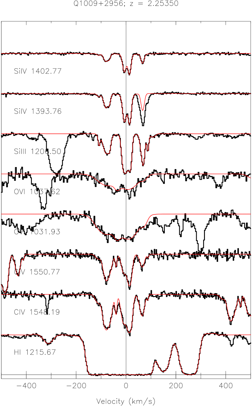
Figure 1: Stacked velocity plot of the $z=2.253$ system in Q1009+2956 (Described in Section 2.5.1 of the text). The thin solid line in this figure and all following velocity plots shows the best-fit model obtained from the VPFIT profile fitting software.

We conclude that the selection of O vi candidate systems based on doublet spacing and ratio, subject to constraints on nearby Ly-$\alpha$ and C iv , is effective at reducing the amount of contamination from the Ly-$\alpha$ forest to $\sim 2$ objects in a sample of 20, or $\sim 10\%$. For the 14 systems with $\Delta v_{{\rm C\;\mbox{\tiny IV}}-{\rm O\;\mbox{\tiny VI}}}<100$ km/s, the identification as O vi should be the most secure, while the contamination may be somewhat worse for the systems showing $100<\Delta v_{{\rm C\;\mbox{\tiny IV}}-{\rm O\;\mbox{\tiny VI}}}<1000$ km/s. Nevertheless, we include these systems in the analysis because of their potential physical importance. Table 2 presents a list of the 18 candidate systems which survived the selection process, along with a summary of basic properties derived from the Voigt profile fitting procedure. The table is organized by system, with columns indicating 1) the system redshift, 2) the number of individual O vi components in the system, 3) the total O vi column density, 4) the number of corresponding H i components with $N_{{\rm H\;\mbox{\tiny I}}}>10^{14.0}$, 5) the column density of the strongest single H i component, 6) the velocity separation between the system and the emission redshift of the background quasar, 7) the velocity separation between the strongest components of O vi and C iv , and 8) The figure number corresponding to the velocity plot for each system. When measuring O vi column densities, we found that the errors on individual components were often somewhat large; this was caused by blending between the components, which opens up a large region of $\chi^{2}$ space where adequate fits can be obtained by trading column density between different lines in the blend. In these cases the total column density is much better constrained than would be inferred from the sum of the errors for individual components. It is this better constrained value that is quoted in Table 2, with accompanying $1\sigma$ errors. Figure 1 presents stacked velocity plots of each system in several ions of interest, overlayed with the best-fit component model.

2.4 General Characteristics of Detected O vi Systems

The properties of our 19 O vi systems are not entirely uniform, and while an interpretation of their physical conditions is not possible without reference to ionization models, there are two classes of systems which can be distingiushed by inspection. The first group of absorbers in this category contains systems that are ejected from the background quasar. We find two such examples in the data (noted in Table 2), and they are characterized by broad absorption that is clearly matched in the O vi 1032Å and 1037Å profiles, but for which the optical depth ratio is too small. This phenomenon has been observed in other high redshift QSOs (Barlow & Sargent, 1997), and is thought to result from partial coverage of the continuum source by small, dense clouds close to the central engine of the QSO. These clouds give rise to saturated absorption over the covered fraction of the central engine, so the doublet ratio approaces unity for these patches. In the uncovered region, unattenuated continuum radiation is able to escape, raising the zero level of the flux to create the appearance of a pair of unsaturated lines with equal strength.

Another group of absorbers which we distinguish from the general population contains systems that are found in the immediate vicinity of the background quasar ($\Delta v<5000$ km/s). The ionization environment of these systems should differ significantly from the general IGM because of the locally enhanced UV radiation field (Weymann et al, 1981). Also, since QSOs are likely to be found in regions of high overdensity the inclusion of this class could skew statistical results because of clustering effects. Four systems (also noted in Table 2) fall into this class, which we hereafter refer to as the “proximity” systems.

After separating out the two populations which are local to the quasar environment, we are left with a total of 12 true cosmological O vi systems, which we call the “intergalactic” sample and which will form the principal focus of this paper. In 10 of these 12 systems, we have detected other highly ionized species within $\Delta v<100$ km/s of O vi , including at least C iv , but usually also Si iii , Si iv and other lower ionization species. These 10 also show strong, saturated Ly-$\alpha$ absorption with $\log N_{{\rm H\;\mbox{\tiny I}}}>14.55$, (for 9 of the 10, $\log N_{{\rm H\;\mbox{\tiny I}}}>15.2$). The identification of these systems as O vi appears to be very secure.

For the remaining 2 intergalactic systems, the O vi absorption is significantly offset from the nearest large concentration of C iv (by $336$ km/s and $772$ km/s). These systems are much more difficult to distinguish from chance Ly-$\alpha$ associations, as there is no closely aligned absorption from any ion other than O vi - including Ly-$\alpha$ and N v . Based on our detection of two reversed doublet systems for which $\Delta v<700$ km/s, these pairs might seem to be likely candidates for contamination. However, the two offset systems differ from the false pairs in that their nearest respective Ly-$\alpha$ systems are exceptionally rich. One shows a cluster of 5 lines with $\log N_{{\rm H\;\mbox{\tiny I}}}>15.5$ within a 700 km/s range, and other has an H i column density of $\log N_{{\rm H\;\mbox{\tiny I}}}=16.0$. Both also exhibit extensive metal line absorption including C iv , Si iv , and Si iii . No reversed doublet systems were observed in the vicinity of such strong Ly-$\alpha$ and C iv , and even the two reversed doublet systems showing $\Delta v_{{\rm C\;\mbox{\tiny IV}}-{\rm O\;\mbox{\tiny VI}}}<1000$ km/s did not have associated Si iv or Si iii . The proximity of the offset O vi candidates to several of the strongest absorption line systems in our survey, along with the fact that the offset velocities are exactly those expected in the infall/outflow scenarios discussed above, have led us to consider these systems as highly probable identifications despite the increased possibility of contamination.

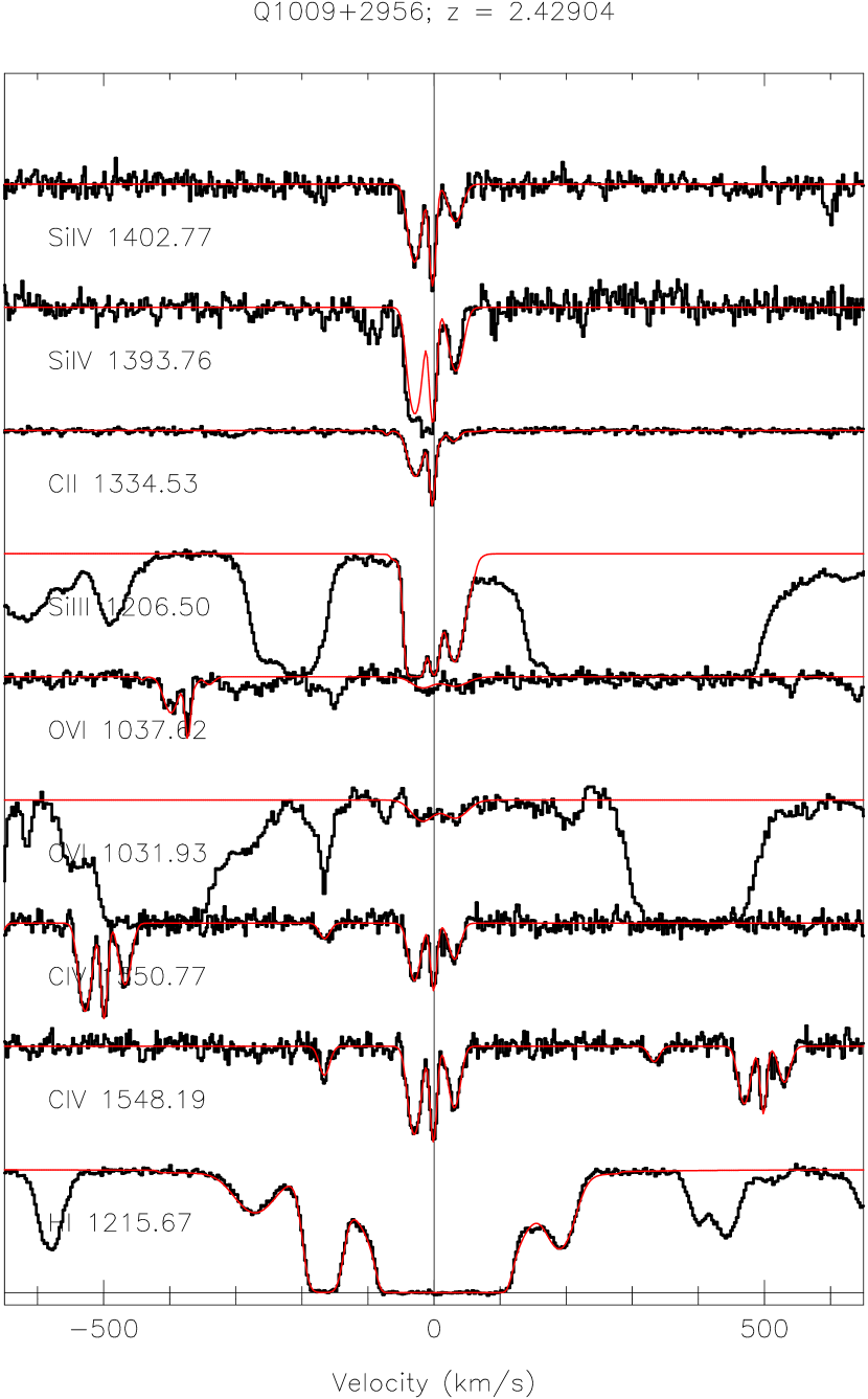
Figure 2: Stacked velocity plot of the $z=2.429$ system in Q1009+2956 (Described in Section 2.5.2 of the text).

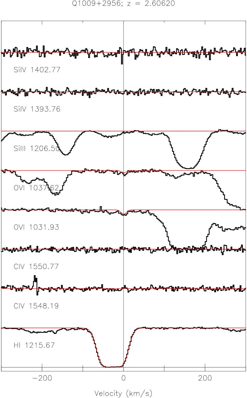
Figure 3: Stacked velocity plot of the $z=2.606$ system in Q1009+2956 (Described in Section 2.5.3 of the text). This system has been excluded from the cosmological statistics due to its proximity to the background quasar.

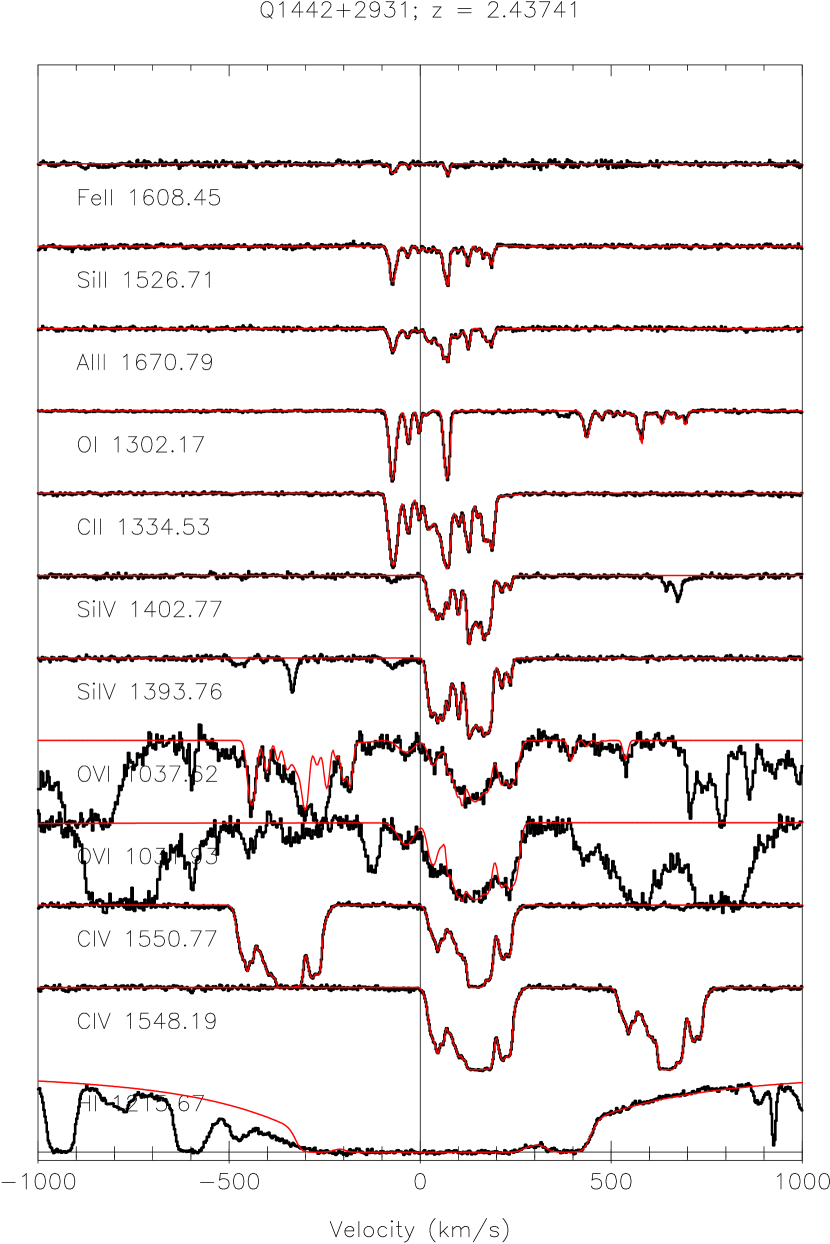
Figure 4: Stacked velocity plot of the $z=2.439$ system in Q1442+2931, which is a weak DLA and the strongest system in the survey (Described in Section 2.5.4 of the text). The additional absorption shown in the O vi 1037Å fit is due to the 1036Å transition of C ii . Likewise, the absorption at +500 km/s in the O i profile is caused by Si ii 1304Å.

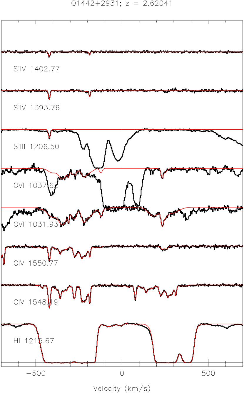
Figure 5: Stacked velocity plot of the $z=2.623$ system in Q1442+2931 (Described in Section 2.5.5 of the text). This system has been excluded from the cosmological statistics due to its proximity to the background quasar.

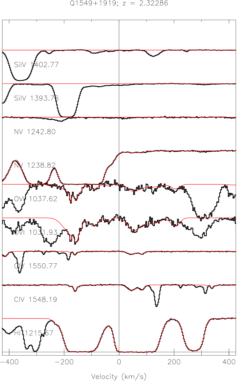
Figure 6: Stacked velocity plot of the $z=2.321$ system in Q1549+1919 (Described in Section 2.5.6 of the text). The O vi 1032Å profile has been adjusted to remove a Ly-$\beta$ line which was blended over the range 0-200 km/s in the figure.

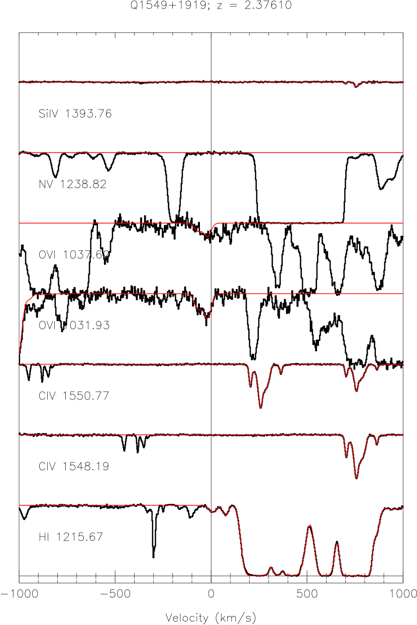
Figure 7: Stacked velocity plot of the $z=2.375$ system in Q1549+1919 (Described in Section 2.5.7 of the text).

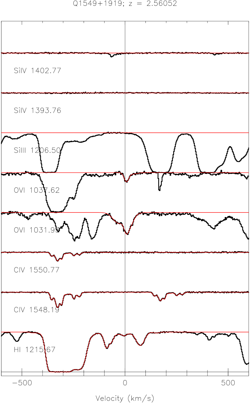
Figure 8: Stacked velocity plot of the $z=2.561$ system in Q1549+1919 (Described in Section 2.5.8 of the text).

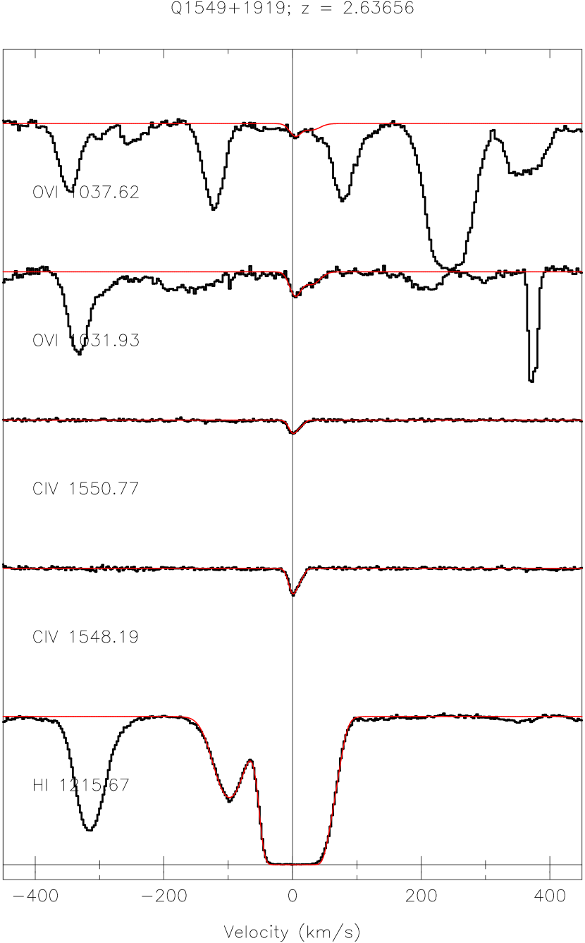
Figure 9: Stacked velocity plot of the $z=2.63$ system in Q1549+1919 (Described in Section 2.5.9 of the text).

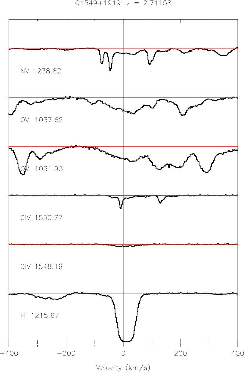
Figure 10: Stacked velocity plot of the $z=2.711$ system in Q1549+1919 (Described in Section 2.5.10 of the text). Because the O vi doublet ratio is unity over the whole profile, we classify this as an ejected system which is partially covering the continuum source.

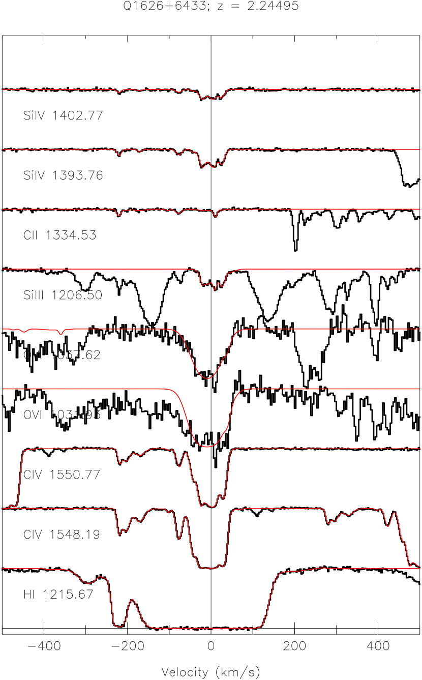
Figure 11: Stacked velocity plot of the $z=2.245$ system in Q1626+6433 (Described in Section 2.5.11 of the text).

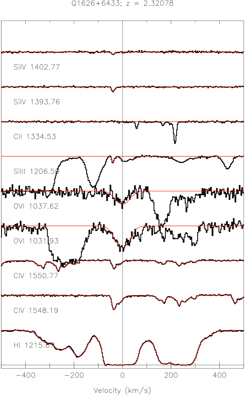
Figure 12: Stacked velocity plot of the $z=2.321$ system in Q1626+6433 (Described in Section 2.5.12 of the text). This system is located 200 km/s redward of the emission redshift of the QSO (measured from Ly-$\alpha$ ). It is therefore excluded from the cosmological statistics, though we believe it is likely caused by the QSO host galaxy itself or a very nearby companion.

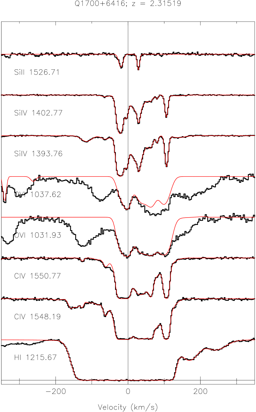
Figure 13: Stacked velocity plot of the $z=2.315$ system in Q1700+6416 (Described in Section 2.5.13 of the text).

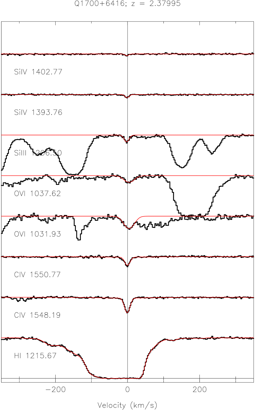
Figure 14: Stacked velocity plot of the $z=2.379$ in Q1700+6416 (Described in Section 2.5.14 of the text).

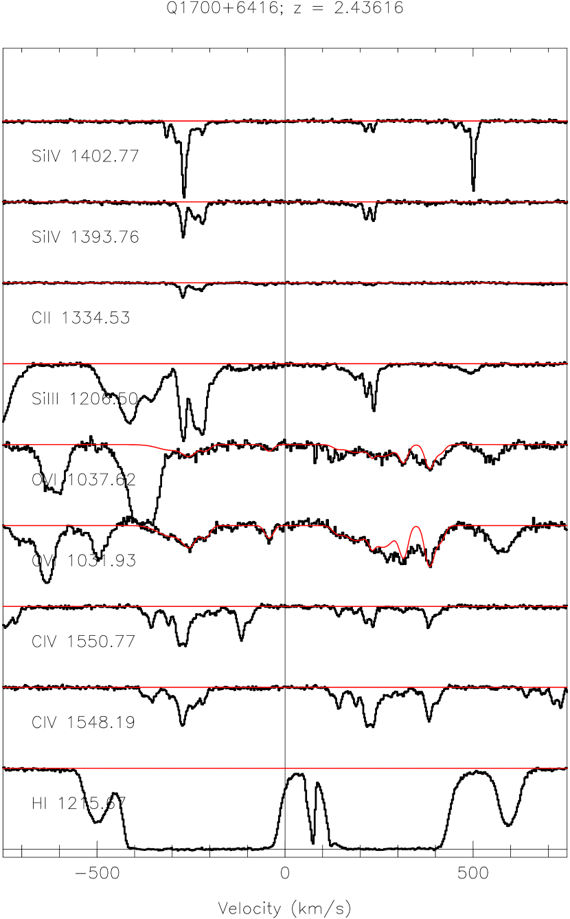
Figure 15: Stacked velocity plot of the $z=2.433/2.439$ system in Q1700+6416 (Described in Section 2.5.15 of the text). The O vi 1032Å profile has been adjusted to remove an interloping Ly-$\beta$ line at $z=2.463$ (+300 km/s), to better illustrate the correspondence of the O vi doublet profiles.

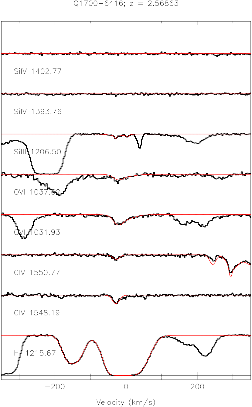
Figure 16: Stacked velocity plot of the $z=2.568$ system in Q1700+6416 (Described in Section 2.5.16 of the text).

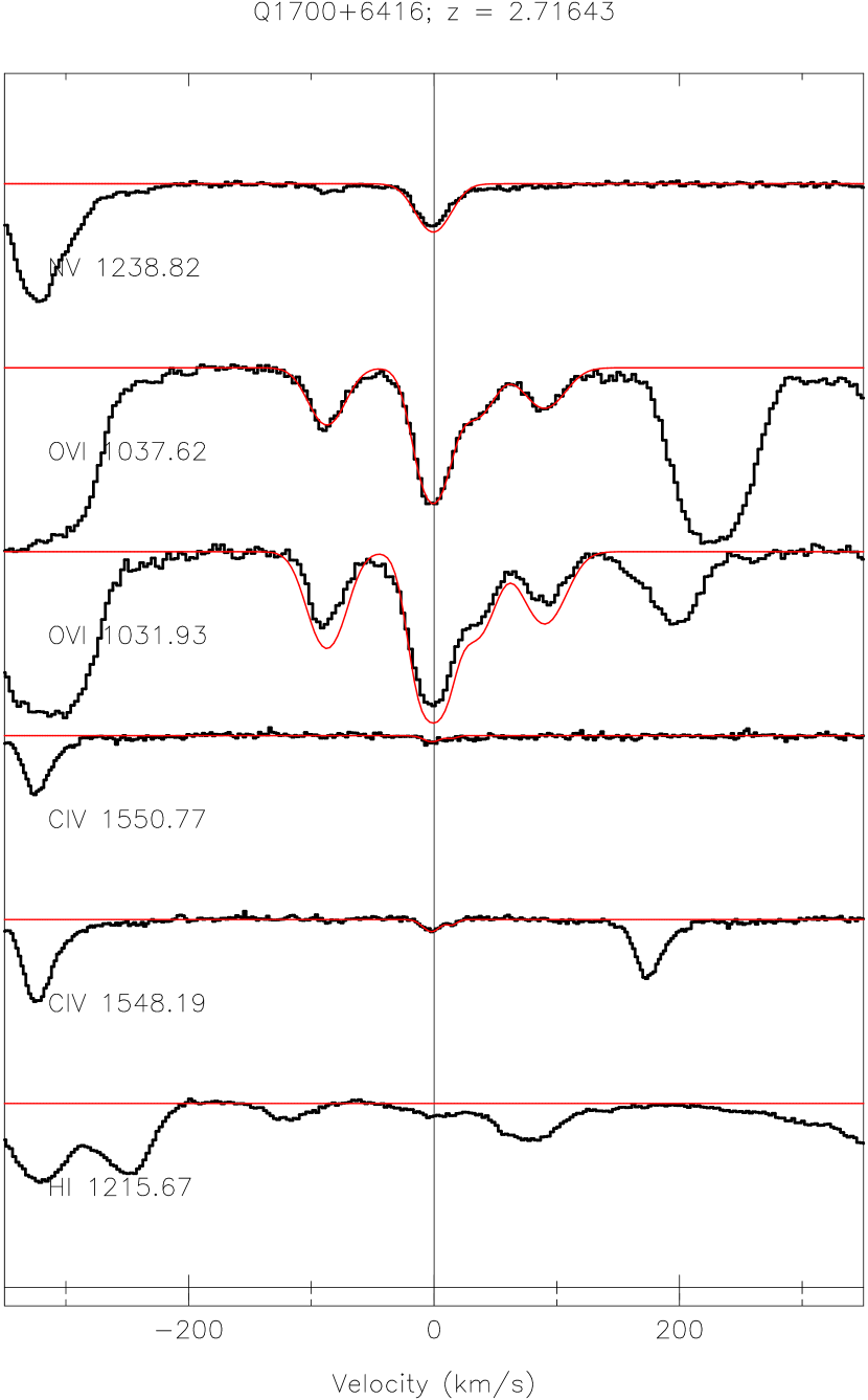
Figure 17: Stacked velocity plot of the $z=2.716$ system in Q1700+6416 (Described in Section 2.5.17 of the text). The model fit shown in the figure illustrates the expected strength of the O vi 1032Å line based on a fit to the 1037Å profile. Because the observed profile does not match the expected doublet ratio, we have surmised that this absorber is ejected from the background QSO and only partially covers the central engine. It has been excluded from the cosmological statistics.

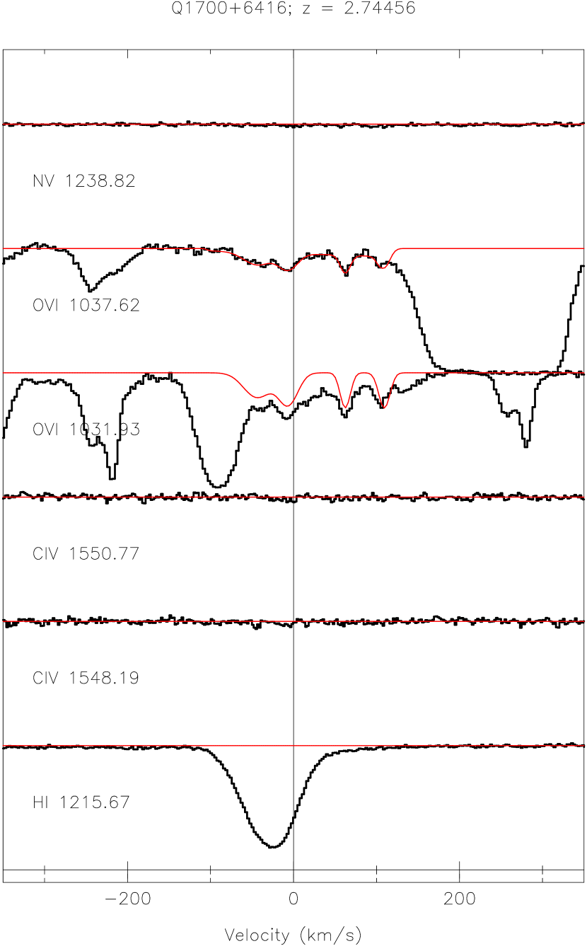
Figure 18: Stacked velocity plot of the $z=2.745$ system in Q1700+6416 (Described in Section 2.5.18 of the text). This system has been excluded from the cosmological statistics sue to its proximity to the background QSO.

From inspection of the final sample of 12 intergalactic systems in Table 2 and Figures 1-18, it is seen that our survey selects primarily strong absorbers, with saturated Ly-$\alpha$ and associated heavy element ions. All of the intergalactic systems show $\log(N_{{\rm H\;\mbox{\tiny I}}})\geq 14.5$ and observable levels of C iv - i.e. we have not detected any “O vi only” absorbers in the forest (although we do see two such cases in the proximity sample). In fact, we have not found a single example of an O vi doublet aligned with a Ly-$\alpha$ forest line in the column density range $13.5<\log N_{{\rm H\;\mbox{\tiny I}}}<14.5$. For many systems, such weak O vi lines would not have been detectable due to variations in the data quality and degree of Ly-$\alpha$ forest blending. Since we have not attempted to deblend lines from Ly-$\alpha$ and higher order H i until after they have already been identified, it is possible that we may be biased against the weakest O vi lines, since these are the first lost to blending from the forest. We have estimated that for lines with similar $N_{{\rm O\;\mbox{\tiny VI}}}$ and $b_{{\rm O\;\mbox{\tiny VI}}}$ to the ones picked out by our selection criteria, our survey is $\approx 40\%$ complete (see Section 3.1.4 for a detailed discussion of the completeness estimation). It is likely that the completeness is lower for the weakest systems - a tradeoff we have made in order to minimize the number of false positive detections in our sample.

Nevertheless, there are several systems in our sightlines where the data is of sufficient quality and the spectrum sufficiently clean of Ly-$\alpha$ lines that we would expect to detect O vi , even at levels nearly an order of magnitude below [O/H]=-2.5 if a Haardt & Madau (1996) shaped UV background is assumed. The detailed question of whether the number of such systems is significant, or whether it is consistent with the expected patchiness in the cosmic metallicity and/or ionizing radiation field is more complex and will be addressed in a companion paper.

Subject to the above caveats, the data and selection techniques presented here do not confirm the presence of photoionized metal lines in the low-density IGM at the [O/H]=-2.5 level . This result comes as a surprise, as previous statistical studies at higher redshift implied a widespread distribution of O vi in association with the forest (Schaye et al, 2000), and theoretical considerations had also pointed to O vi searches as the most effective way to test the widespread enrichment hypothesis (Chaffee et al, 1986; Rauch et al, 1997a; Hellsten et al, 1998). Our results agree more closely with those of Dave et al (1998), who find a significant downward gradient in metallicity toward low density regions of the IGM at $z\sim 3.25$. For the remainder of this paper, we limit the discussion to the strong systems which have been firmly identified in the survey.

2.5 Observed Properties of Individual Systems

In this section we present brief summaries of the notable spectral features in each O vi system. We limit the present discussion to actual observed properties; further discussion of the absorbers’ physical conditions is given in Section 3. The systems are organized by sightline, in order of increasing redshift.

2.5.1 Q1009+2956: $z=2.253$ (Figure 1)

Our first O vi candidate is located in the vicinity of a strong Lyman limit system (LLS, $\log N_{\rm{\rm H\;\mbox{\tiny I}}}=17.8$). Both Ly-$\alpha$ and Ly-$\beta$ were used to fit for the H i column density; higher order Lyman transitions could not be used due to the presence of another Lyman Limit system at higher redshift. Complex chemical absorption containing C iv , Si iv , and Si iii and spanning roughly 200 km/s is associated with the strongest H i absorption. The velocity structure in these ions is closely aligned, although the C iv /Si iv ratio varies across the profile, suggesting a spatial variation in ionization conditions. Our Voigt profile fits indicate that the alignment and relative widths of C iv and Si iv are consistent with pure thermal broadening of the profile at $T_{C,Si}=0.8-1.2\times 10^{5}$ K (reflecting the range for different individual components).

The O vi profile differs markedly from those of Si iv and C iv , and is characterized by a broad trough with little substructure. This smooth, blended nature causes the Voigt fit parameters to be poorly constrained - particularly the line widths. For this reason, and also because of blended Ly-$\alpha$ forest absorption in the O vi 1037 Å profile (seen to the blue in Figure 1a) any detailed physical conclusions about the O vi gas remain tentative. However, it is still evident from inspection of the profiles that the small amount of structure in the O vi line does not mirror that of C iv and Si iv . Taking the best-fit Voigt parameters at face value, the measured limits on the O vi temperature range from $T_{{\rm O\;\mbox{\tiny VI}}}\leq 0.2-2.1\times 10^{6}$ K for various components, or roughly an order of magnitude above the measured temperatures for C iv and Si iv .

2.5.2 Q1009+2956: $z=2.429$ (Figure 2)

This system is dominated by a single strong H i component, whose column density was measured at $\log(N_{\rm H\;\mbox{\tiny I}})=17.687$ using Ly-$\alpha$ ,$\beta,\gamma$ and $\delta$. As expected for such a strong H i system, significant absorption is present in lower ionization species including C ii , Si ii , and Al ii . The C iv , Si iv , and Si iii profiles are closely aligned, and contain at least one very narrow ($b_{{\rm C\;\mbox{\tiny IV}}}=4.8$ km/s) component that aligns with C ii and implies a temperature of $T<14,000$ K. Similar linewidths for the Si iv and C iv profiles indicate that their broadening may be largely non-thermal, and the temperatures even lower.

The O vi profile contains two subcomponents, neither of which align in velocity with the lower ionization lines. Their line widths of $b_{{\rm O\;\mbox{\tiny VI}}}=22.2,24.7$ km/s imply upper limits of $T_{{\rm O\;\mbox{\tiny VI}}}<5\times 10^{5}$ K.

2.5.3 Q1009+2956: $z=2.606$ (Figure 3)

This system consists of a single, isolated Ly-$\alpha$ line with associated O vi , but no absorption from any other heavy elements. The H i resembles a typical Ly-$\alpha$ forest line, at $\log(N_{{\rm H\;\mbox{\tiny I}}})=14.442$ and $b_{{\rm O\;\mbox{\tiny VI}}}=25.6$ km/s. A single O vi line is detected at the $\geq 3\sigma$ level, and is measured to have $\log(N_{{\rm O\;\mbox{\tiny VI}}})=12.709$ and $b_{{\rm O\;\mbox{\tiny VI}}}=8.0$ km/s ($T_{{\rm O\;\mbox{\tiny VI}}}\leq 6.2\times 10^{4}$ K). This is an example of the type of system we had expected to detect in large numbers in our survey. However, this particular absorber is located only 3050 km/s from the background quasar and its ionization state is likely to be affected by UV radiation from the QSO. It has therefore been grouped with the “proximity” sample and not included in our discussion of cosmological O vi absorbers. However, its detection illustrates that the survey is sufficiently sensitive to uncover O vi only systems, even though we have found none in the more tenuous regions of the IGM.

2.5.4 Q1442+2931: $z=2.438$ (Figure 4)

This O vi absorption is associated with a weak damped Ly-$\alpha$ (DLA) system. The damping wings of the profile spread over several echelle orders, complicating attempts to determine the exact H i column density. However, based on the presence of the modest damping wings, and a relatively weak saturation level in the core by DLA standards, we estimate that $\log N_{{\rm H\;\mbox{\tiny I}}}\sim 19.0-20.0$. A rich metal line structure is detected both in low ionization (O i , Si ii , Fe ii , Al ii , C ii ) and high ionization (C iv , Si iv ) species. The kinematic spread of the lowest ionization gas (e.g. Fe ii , O i ) spans a range of $\sim 200$ km/s and is centered near the strongest H i absorption. The highest ionization gas (C iv , Si iv , O vi ) also spans a $\sim 200-250$ km/s velocity interval, but is offset $\sim 200$ km/s to the red of the low ionization species. Several intermediate ionization lines (Si ii , C ii , Al iii ) bridge the velocity range between the high and low ionization species, sharing absorption components with both varieties of gas.

The O vi kinematics strongly resemble those of C iv , where a strong absorption trough at $z=2.390$ is flanked by two weaker structures at $\pm 100$ km/s. A detailed comparison of the central regions of the profiles is not possible because of saturation in the C iv core.

2.5.5 Q1442+2931: $z=2.623$ (Figure 5)

This O vi absorption is associated with a pair of strong H i systems, seen at $\sim\pm 300$ km/s in Figure 1f. The H i at $-300$ km/s splits into three strong components in higher order Lyman lines, and we measure these to have column densities of $\log(N_{{\rm H\;\mbox{\tiny I}}})=15.3,15.3,$ and $14.6$. The group at $+300$ km/s is dominated by a single line with $\log(N_{{\rm H\;\mbox{\tiny I}}})=15.8$. The whole complex is located near the background quasar at $\Delta v\approx 3100$ km/s, so we have grouped it in the proximity sample and excluded it from our cosmological statistics.

This system was originally identified as an O vi absorber based on the narrow line located near +250 km/s in the figure. Though this line is blended with Ly-$\alpha$ absorption from the forest in the 1032 Å component, a sharp core is quite visible in the profile that mirrors the shape of the uncontaminated O vi 1037 A line. The width of this core is relatively small at $b=7.41$ km/s, and implies an upper limit of $T_{{\rm O\;\mbox{\tiny VI}}}\leq 5.27\times 10^{4}$ K. A second, much broader component ($b=19$ km/s) is also seen in the red wing of this line. C iv is detected in the same velocity range as the sharp O vi component, further securing the O vi identification for the system. The O vi and C iv may come from the same gas, as the redshifts are identical to within the $1\sigma$ errors, and the velocity widths are also within $1\sigma$ of a simulateneous solution of $T_{{\rm C\;\mbox{\tiny IV}},{\rm O\;\mbox{\tiny VI}}}=8.5\times 10^{4}$ K. The column density ratio for these lines is $\log(N_{{\rm O\;\mbox{\tiny VI}}}/N_{{\rm C\;\mbox{\tiny IV}}})=0.454$.

The absorption complex at $-300$ km/s shows a much richer chemical structure, containing kinematically complex C iv , and also weak Si iv and Si iii . We did not originally identify O vi associated with this H i using our search strategy, because we could not be certain that much of the absorption in the 1037 Å profile over this range was not Ly-$\alpha$ contamination. However, in light of the nearby sharp O vi line discussed in the preceeding paragraph, the strong H i , C iv , Si iv , and Si iii , and the good match of the 1032 Å and 1037 Å profiles, we treat this as a possible, or tentative O vi identification. If this absorption actually represents O vi , its properties are different from those of the C iv and Si iv lines. Solving simultaneously for the temperature using the C iv and Si iv linewidths , we find $T_{C,Si}=1.2-2.6\times 10^{4}$ K, while attempts to fit the O vi profile yield linewidths in the range $b_{{\rm O\;\mbox{\tiny VI}}}=10.6-32.8$ km/s, or $T_{{\rm O\;\mbox{\tiny VI}}}\leq 1\times 10^{5}-1\times 10^{6}$ K. This system appears not to be unique in its association with a group of strong H i and metal lines rather than a single strong system (See for example Section 2.5.15).

2.5.6 Q1549+1919: $z=2.320$ (Figure 6)

This example contains a broad complex of O vi distributed over $\Delta v\sim 500$ km/s. The associated H i is once again not dominated by a single line, but rather by a cluster of three moderately strong lines ($\log N_{{\rm H\;\mbox{\tiny I}}}=15.195,14.627,14.111$) within a small velocity interval. The O vi in this system was originally identified by the presence of two narrow lines seen at the blue end of the profile. We detect a single weak C iv line associated with this narrow O vi component. Although the C iv and O vi do not align exactly in velocity, their doppler widths both indicate upper limits on the temperature which are quite cool, in the range $T\leq 3.2-7.4\times 10^{4}$ K. One of the O vi lines is extremely narrow at $1.46$ km/s ($T_{{\rm O\;\mbox{\tiny VI}}}\leq 2000$ K), although this may be a noise artifact.

A second pair of C iv lines is detected near the strongest Ly-$\alpha$ line in the system. This additional C iv is unusually broad and featureless - the velocity width of one of the two C iv components is measured at $b=19.67$ km/s, or $T_{{\rm C\;\mbox{\tiny IV}}}\leq 2.8\times 10^{5}$ K. Such an environment should be conducive to the production of other very highly ionized species, including O vi . However, we did not at first identify any O vi associated with the broad C iv because the O vi 1032 Å line was blended with a higher redshift Ly-$\beta$ line. The contamination was removed by fitting the corresponding Ly-$\alpha$ profile to infer the Ly-$\beta$ line strength, revealing the profile shown in the figure.

The shape of the deblended profile suggests that O vi exists over the entire range of H i absorption. Most of this O vi is lacking in detailed substructure. Our Voigt profile fits help to characterize several of the apparently broad features, although the errors on the fit parameters are significant because of the smoothness of the profile. The strongest distinct feature is a broad line near the strongest H i component and wide C iv ($+50$ km/s in Figure 6). Its measured $b_{{\rm O\;\mbox{\tiny VI}}}=26.43$ implies an upper limit on the temperature of $T\leq 6.7\times 10^{5}$ K. This matches the high temperature inferred from C iv to within $1\sigma$ errors, although the different shapes of the O vi and C iv profiles indicate that the absorption probably does not arise in the same gas.

2.5.7 Q1549+1919: $z=2.376$ (Figure 7)

This system is offset by more than $700$ km/s from the nearest C iv line. No absorption is seen from any ion including H i at the O vi redshift, so the identification rests on the similarity of the doublet profiles alone. These are identical to within the noise over most of their length, though some blending is present in the 1037Å component.

The nearest H i to this system is an unusual complex, containing five lines of $\log(N_{{\rm H\;\mbox{\tiny I}}})>14.0$ within a span of $600$ km/s. No single line dominates the complex; the strongest (located at $+750$ km/s from the O vi ) is measured at $\log(N_{{\rm H\;\mbox{\tiny I}}})=15.6$. C iv , Si iii , and Si iv are clearly detected in association with the strongest H i component, but the O vi profile suffers from heavy Ly-$\alpha$ forest blending in this region. Using profile fits of the C and Si ions to solve simulatneously for the gas temperature and non-thermal motions, we estimate $T_{C-Si}=2.2\times 10^{4}$ K.

Our best fit Voigt profile for the O vi (based primarily on the unblended 1032 Å component) requires two lines, with widths of $b=25.24,26.70$ km/s. The implied upper limits on the O vi temperature are $T_{{\rm O\;\mbox{\tiny VI}}}\leq 6.5\times 10^{5}$ K - over an order of magnitude higher than that of C or Si, although the O vi measurement is only an upper limit. High quality data in the C iv and N v regions ($\frac{S}{N}({\rm C\;\mbox{\tiny IV}})\approx 150,\frac{S}{N}({\rm N\;\mbox{\tiny V}})\approx 120$ per pixel) allow to set extremely strong limits on the non-detection of other ions associated with O vi : in particular $\log(N_{{\rm O\;\mbox{\tiny VI}}}/N_{{\rm N\;\mbox{\tiny V}}})>2.398$ and $\log(N_{{\rm O\;\mbox{\tiny VI}}}/N_{{\rm C\;\mbox{\tiny IV}}})>2.717$.

2.5.8 Q1549+1919: $z=2.560$ (Figure 8)

This system contains a single O vi line with no associated H i absorption, although a strong H i absorber of $\log(N_{{\rm H\;\mbox{\tiny I}}})=15.219$ is located $336$ km/s to the blue. The O vi 1032 Å line is blended with interloping H i , but a distinct narrow component is still visible in this blend, matching in redshift and doppler parameter with the clean O vi 1037 Å profile. The measured $b_{{\rm O\;\mbox{\tiny VI}}}=14.6$ km/s translates to an upper limit of $T_{{\rm O\;\mbox{\tiny VI}}}\leq 2.0\times 10^{5}$ K.

As in the preceding example, no absorption is seen from any other heavy elements at the redshift of the confirmed O vi : we measure limits of $\log(N({\rm O\;\mbox{\tiny VI}})/N({\rm C\;\mbox{\tiny IV}}))\geq 2.701$ and
$\log(N({\rm O\;\mbox{\tiny VI}})/N({\rm N\;\mbox{\tiny V}}))\geq 2.038$. However, a significant amount of C iv is associated with the Ly-$\alpha$ complex at $-336$ km/s. In this region, the detailed structure of the O vi 1032 Å profile seems to mirror that of the C iv , suggesting that there may be further O vi locked up in this system. Indeed, the observed O vi substructure is almost certainly not the product of chance Ly-$\alpha$ forest absorption, as it varies on velocity scales of $\sim 10$ km/s, whereas characteristic velocity widths in the Ly-$\alpha$ forest are $b>20$ km/s. Nevertheless, we do not claim a direct detection of O vi in this part of the profile, as the O vi 1037Å line is saturated by a blended Ly-$\alpha$ forest line, and further examination of the 1032Å component indicates that it suffers from blending as well.

2.5.9 Q1549+1919: $z=2.636$ (Figure 9)

This system has a particularly simple chemical and velocity structure. The Ly-$\alpha$ profile is dominated by a single H i line with $\log(N_{{\rm H\;\mbox{\tiny I}}})=15.220$, which places it among the weakest systems in the survey. Several other systems contain groups of lines with similar H i column densities, but this system is unusual in its isolation from other strong H i .

Heavy element absorption is only seen in C iv and O vi , both of which are adequately fit by a pair Voigt profile components. The velocity alignment between the ions is relatively close, but for both components the O vi linewidth exceeds that of C iv despite the fact that O vi is a heavier ion than C iv . The C iv linewidth constrains its temperature to be below $T_{{\rm C\;\mbox{\tiny IV}}}<5.0\times 10^{4}$ K, while the O vi linewidth permits temperatures in the range $T_{{\rm O\;\mbox{\tiny VI}}}<1.3,2.6\times 10^{5}$ K for the two components.

2.5.10 Q1549+1919: $z=2.711$ (Figure 10)

This absorber is an example of highly ionized ejecta from the background QSO, moving at $v_{ej}\approx 10,000$ km/s. A wide, sloping absorption profile is seen in O vi , C iv , and N v (only N v 1238 Å is shown, as the 1242 Å line is contaminated). The H i seen at the same redshift is not likely to be associated with the ejecta, as it shows no sign of the unusual kinematics that characterize the high ionization lines. The principal evidence for the ejection hypothesis comes from the doublet ratios of O vi , C iv , and N v , which are unity over their whole profiles rather than the value deduced from the oscillator strengths of different transitions (see Section 2.4 for a more thorough discussion of this phenomenon). Accordingly, we have excluded this system from our further statistical analysis.

2.5.11 Q1626+6433: $z=2.245$ (Figure 11)

This O vi system - our lowest redshift example - is somewhat difficult to interpret due blending and saturation in the O vi 1032 Å component, and a relatively low signal-to-noise ratio ($\sim 7$). It is associated with a multicomponent H i complex of total column density $\log(N_{{\rm H\;\mbox{\tiny I}}})=15.544$ seen as a single line in Ly-$\alpha$ , although a fit to Ly-$\beta$ reveals several subcomponents. The strongest of these is saturated in both Ly-$\alpha$ and Ly-$\beta$ , but higher order transitions could not be used in the fit because of their poor signal-to-noise ratios.

Heavy element absorption is seen in C ii , C iv , Si iv , and Si iii . In each case, the metals are in two clusters - one associated with the densest H i , and a second, weaker group near a smaller H i line at $-200$ km/s. The O vi absorption is only found near the stronger line, though a weak signal at $-200$ km/s could be masked by noise. Since the strong C iv profile is saturated in the 1548Å component, we have used only the unsaturated 1551Å component to measure the velocity profile. The individual elements of the C iv , Si iii , and Si iv absorption align well in velocity, and the fits indicate a temperature range of $T=2-8\times 10^{4}$ K for the Carbon and Silicon gas.

Because of lower data quality, it is difficult to judge whether the velocity structure of O vi matches that of the C iv and Si iv profiles. The overall velocity extent appears to be similar, but any substructure is lost in the noise. We have therefore compared two different approaches to measure the system’s properties. The first of these assumes that the O vi absorption comes from the same gas as C iv , Si iii , and Si iv , and is motivated by the similar extent of O vi and C iv in velocity space. To test the plausibility of this hypothesis, we have fit a model O vi profile that contains 8 components with the same redshifts and $b$ parameters (reweighted by $\sqrt{m_{{\rm C\;\mbox{\tiny IV}}}/m_{{\rm O\;\mbox{\tiny VI}}}}$) as the C iv profile. The column densities were then allowed to vary to achieve the best fit. The O vi line strengths measured in this way yield typical ratios of $\log(N_{{\rm O\;\mbox{\tiny VI}}}/N_{{\rm C\;\mbox{\tiny IV}}})\sim 0.3$ and $\log(N_{{\rm O\;\mbox{\tiny VI}}}/N_{{\rm Si\;\mbox{\tiny IV}}})=1.5-2.2$ for individual absorption components. We then compared these ratios with the predictions of ionization simulations (described in detail in section 3.1.3) to see if they are consistent with a photoioniation interpretation. From this exercise we found that if the C iv and Si iv are produced in the same gas, then the observed O vi line strength is much stronger then expected. We therefore consider it likely that the O vi gas is physially distinct from the C iv and Si iv gas, which is similar to what is seen in most other systems.

Our second approach assumes that the C and Si absorption are associated, but that the O vi is contained in a separate phase. A Voigt profile fit to the O vi 1037Å profile requires only two components to adequately represent the data ($\chi^{2}_{\nu}=1.02$). The fit does not match the 1032 Å profile exactly, but the discrepancy can be attributed to forest contamination. Most of the O vi absorption is contained in a single component with $\log(N_{{\rm O\;\mbox{\tiny VI}}})=14.8$ and $b_{{\rm O\;\mbox{\tiny VI}}}=38$ km/s ($T_{{\rm O\;\mbox{\tiny VI}}}\leq 1.4\times 10^{6}$ K). This total column density is actually quite similar to the total column measured using the first approach, but the upper limit on the temperature is significantly higher. This second hypothesis can be plausibly reconciled with collisoinal ionization predictions, so we consider it to be the more likely of the two scenarios.

2.5.12 Q1626+6433: $z=2.321$ (Figure 12)

This unusual system is actually located 300 km/s redward of the Ly-$\alpha$ emission line of the QSO, an effect that can be caused by a 300-500 km/s blueshift of of the Ly-$\alpha$ emission line relative to the “true” QSO redshift as measured from narrow forbidden lines (Tytler & Fan, 1992). However, the properties of this system favor its interpretation as an intervening rather than ejected absorption system. Ultimately we do not include it in the cosmological sample because of its proximity to the background quasar.

The H i structure consists of a group of four moderately strong lines ($14.0<\log N_{{\rm H\;\mbox{\tiny I}}}<15.5$) within a $\Delta v\sim 500$ km/s velocity interval - similar to what is seen in many of the other O vi absorbers we have detected. C iv , Si iii , Si iv , and O vi are all seen in the vicinity of the central, strongest H i line and the velocity structure in all of these ions is identical except for O vi . The velocity profiles of the moderate ionization lines are consistent with their production occurring in a single common gas phase at $T=2.25\times 10^{4}$ K.

The O vi profile is much stronger and broader than those of all the other observed species. A single $b_{{\rm O\;\mbox{\tiny VI}}}=37$ km/s Voigt profile provides our best fit to the data, and sets an upper bound on the temperature of $T_{{\rm O\;\mbox{\tiny VI}}}\leq 1.3\times 10^{6}$ K - almost two orders of magnitude higher than the lower ionization species.

One could interpret the large velocity width of O vi , and its high ionization state as a sign that the O vi gas is ejected from the QSO rather than intervening. While this possibility cannot be disproven, the 300 km/s redshift of the O vi line relative to Ly-$\alpha$ requires that the ejection velocity $v_{ej}\leq 200$ km/s even after including a +500 km/s correction to the Ly-$\alpha$ redshift. This velocity is very small compared to values of several thousand km/s typical of material ejected from QSOs (Turnshek, 1984). Furthermore, the close alignment of the O vi and other ions ($\Delta v<40$ km/s), the accuracy of the doublet ratio implying full coverage of the continuum source, and the quiescent kinematics of C iv and other lower ionization species, all point away from the ejection hypothesis for this absorber. We favor the interpretation that the absorption arises in intervening gas, possibly associated with the QSO host galaxy or a nearby companion.

2.5.13 Q1700+6416: $z=2.316$ (Figure 13)

This O vi absorption is associated with a Lyman limit system, of column density $\log(N_{{\rm H\;\mbox{\tiny I}}})=17.6$, although only Ly-$\alpha$ and Ly-$\beta$ could be used in the measurement and both were saturated. Rich heavy element absorption is seen in both high ionization species (C iv , Si iv , and O vi ) and low ionization species (C ii , Al ii , Si ii ).

The low ionization species all share a similar kinematic structure, concentrated around two lines separated by $\sim 45$ km/s in the very core of the H i profile. The narrow widths of these lines imply low temperatures in the range $T_{{\rm O\;\mbox{\tiny VI}}}\leq 0.7-7\times 10^{4}$ K, as would be expected in the central regions of a strong H i system.

The highly ionized species are very strong, and in the case of C iv we observe significant saturation. The velocity structure of the gas can be read from the Si iv line, which appears to match the C iv profile but is probably not related to O vi . The temperature of the C-Si phase derived from the Si iv line widths is quite cool, and resembles that of the low ionization gas at $T\leq 2-3\times 10^{4}$ K. However, the moderate ionization species are much more widespread, spanning $\sim 150$ km/s. The O vi profile is significantly contaminated by Ly-$\alpha$ forest absorption, particularly in the 1037 Å component. At least one line, located at $-20$ km/s in the Figure 1n, is clearly distinguished and may be associated with the strongest C iv and Si iv lines even though the redshifts do not align exactly. Our best-fit Voigt profile for this line contains two components, with $b$ parameters of $14.35$ and $11.53$ km/s ($T_{{\rm O\;\mbox{\tiny VI}}}=1.27-1.97\times 10^{5}$ K) and column densities of $\log(N_{{\rm O\;\mbox{\tiny VI}}})=14.0,14.2$. The column densities derived from fitting the rest of the profile are all similar, though the linewidths are larger ($b=15-25$ km/s). While this may be an indication of higher temperature gas, the model for this part of the O vi profile is highly uncertain because of the strong forest contamination.

2.5.14 Q1700+6416: $z=2.379$ (Figure 14)

This is the most kinematically simple O vi system we have detected in our survey; each of the observed metal lines contains only a single absorption component. The H i line is at the strong end of the Ly-$\alpha$ forest regime, with two dominant components at $\log(N_{{\rm H\;\mbox{\tiny I}}})=14.8,15.4$. Besides O vi , we detect most of the common high ionization species, including C iv , Si iii , and Si iv , however no N v is detected. We also do not see any low ionization lines.

Our fits to the Si and C lines may be accurately explained with a single gas phase, with $T_{C,Si}=3\times 10^{4}$ K, characteristic of low density gas in the Ly-$\alpha$ forest. The O vi line differs from these other species slightly in both redshift, which is offset by 10 km/s (a $6\sigma$ difference), and doppler width, measured at 19 km/s. This width admits the possibility of a high termperature gas, i.e. $T_{{\rm O\;\mbox{\tiny VI}}}\leq 3.4\times 10^{5}$ K. Although one might expect some uncertainty in the line widths because of blending in the O vi 1032 line, we have used only the 1037 A component of the doublet in our fit, and found that it matches the 1032 Å profile extremely well. The measured column densiy ratios for O vi , and Si iv are $\log(N_{{\rm O\;\mbox{\tiny VI}}}/N_{{\rm C\;\mbox{\tiny IV}}})=0.323$, and $\log(N_{{\rm O\;\mbox{\tiny VI}}}/N_{{\rm Si\;\mbox{\tiny IV}}})=1.570$. As was discussed in Section 2.5.12, these ratios do not agree with the predictions of simple photoionization models for C iv and Si iv , so it is quite likely that the O vi is physically distinct from these other species.

2.5.15 Q1700+6416: $z=2.436$ (Figure 15)

This complex system contains a number of lines distributed over $\sim 1000$ km/s. The lines are grouped into two distinct clusters separated by $\sim 5-600$ km/s, and each cluster contains absorption from both low ionization species (e.g. C ii ) and high ionization species, including C iv , Si iii , Si iv , and O vi .

The H i absorption in this system contains 8 lines with $\log(N_{{\rm H\;\mbox{\tiny I}}})>14.0$ in a $1000$ km/s velocity interval. The H i near the blue line cluster is dominated by a single line with $\log(N_{{\rm H\;\mbox{\tiny I}}})=16.943$. The red cluster’s H i splits into several components in the higher order Lyman lines, and is dominated by three lines with $\log(N_{{\rm H\;\mbox{\tiny I}}})=14.860,15.706$, and $15.806$. The sharp line seen between the two strong H i features is an unrelated Si iii 1206 line at $z=2.463$.

In both of the line clusters, blending from the Ly-$\alpha$ forest complicates the measurement of O vi parameters. This is apparent for the absorption at $-300$ km/s in Figure 1p, for which the 1037Å component is blended with a strong H i line. Though not obvious in the Figure, it is also true for the absorption at $+300$ km/s, which is blended with a $z=2.46$ Ly-$\beta$ line. By fitting the corresponding Ly-$\alpha$ line ($\log(N_{{\rm H\;\mbox{\tiny I}}})=14.4$), we were able to remove the Ly-$\beta$ contamination, revealing the profile shown in the figure.

Kinematically complex C iv is seen in the neighborhood of each of the absorption clumps, and Si iii and Si iv are also strong, through not as distributed in velocity. Low ionization species (C ii and Si ii ) are seen in the same vicinity as some Si iii and Si iv , though only near the strongest of the H i lines in the blue line cluster. The linewidths of the low and moderate ionization gas are consistent with thermal broadening at $T=4-7\times 10^{4}$ K.

The kinematics of the O vi gas are more difficult to constrain because of Ly-$\alpha$ forest contamination. For the blue line cluster, we have treated all the absorption in the O vi 1032 Å line as actual O vi . Under this assumption, a three component model is sufficient to describe the data. Two of the components can be matched to the 1037 Å profile in the wing of the blended Ly-$\alpha$ , but the third component is completely blended and therefore more suspect. All three of the lines are broad; the doppler widths for the two secure lines are $b_{{\rm O\;\mbox{\tiny VI}}}=22.14,23.48$ km/s, or $T_{{\rm O\;\mbox{\tiny VI}}}\leq 5.3\times 10^{5}$ K. In the redder cluster of lines, the velocity widths are difficult to measure because the profile is not easily described by discrete lines. Our best-fit model again shows lines that are broader than those of other ions, near $b_{{\rm O\;\mbox{\tiny VI}}}=15$ km/s or $T_{{\rm O\;\mbox{\tiny VI}}}\leq 2.2\times 10^{5}$ K. One line is much broader yet at $40$ km/s.

2.5.16 Q1700+6416: $z=2.568$ (Figure 16)

This system has a simple velocity structure, and is centered near a moderate Ly-$\alpha$ absorber ($\log N_{{\rm H\;\mbox{\tiny I}}}=14.5$). A single, narrow heavy element line with weak flanking absorption is seen in C iv and Si iii ; a very weak Si iv feature is also detected, but is not strong enough to provide detailed velocity information. The C iv linewidth is an intermediate $b=12.9$ km/s ($T\leq 1.2\times 10^{5}$), while Si iii is very narrow, implying $T\leq 2\times 10^{4}$ K.

The shapes of the O vi 1032 and O vi 1037 Å components do not match in detail, probably because of blending in the 1032 Å line. The O vi 1037 line profile does however resemble the shape of C iv , although our best fit shows it to be offset by 10-12 km/s. Our estimate of 17.8 km/s for the O vi linewidth implies a higher temperature for the O vi gas, with an upper limit of $T\leq 3.0\times 10^{5}$ K. However, we caution that blending in the O vi core makes it difficult to obtain a reliable measurement of the width. While the coincidence with C iv increases the probability of this system being O vi , we still regard its identification as tentative.

2.5.17 Q1700+6416: $z=2.716$ (Figure 17)

The system is another example of gas ejected from the background quasar, in this case at 2250 km/s. The system was identified by an unmistakable correspondence between the profiles of the O vi doublet components. Strong absorption is seen in O vi , C iv , and N v , and in each case the ratio of the line strengths for the two components of the doublet is smaller than the expected value, indicating partial coverage of the continuum source. Because this is an ejected rather than intervening source, we have excluded it from further analysis.

2.5.18 Q1700+6416: $z=2.744$ (Figure 18)

The last system we discuss contains four distinct components, neighboring a single weak H i line. No heavy elements other than O vi are detected. The measured linewidths for the three O vi components range from $7.14$ km/s to $15.27$ km/s ($T_{{\rm O\;\mbox{\tiny VI}}}\leq 5\times 10^{4}-2.2\times 10^{5}$ K. Since this system is extremely close to the background QSO, we do not include it in our cosmological statistics. The quasar is known to be ejecting O vi (see previous section), so the absorption could be caused by additional outflow.

3 Analysis

3.1 The Physical Environment of O vi Absorbers

The production of O vi is thought to take place in two very different environments: either low density, photoionized plasmas such as would be found in the Ly-$\alpha$ forest, or shock heated, collisionally ionized plasmas, as would be found at the interface between dense structures and the general IGM. The common association we observe between O vi absorbers and strong, metal-rich H i systems causes us to favor a priori the second hypothesis. In the following sections, we draw comparisons between the measured properties of the O vi absorption and the predictions of ionization simulations to see if the two are consistent with this qualitative conclusion.

For the ionization calculations, we have used the CLOUDY96 software package (Ferland et al, 1998). The gas was modeled as an optically thin plane-parallel slab in the presence of a Haardt & Madau (1996) shaped ionizing background spectrum for $z=2.5$. The intensity of the ionizing background was normalized to $J_{-21}=1.0$ (Scott et al, 2000), and the gas assumed to have a metallicity of $Z=\frac{1}{10}Z_{\sun}$ with solar relative abundances for the heavy elements. A grid of models was then computed by varying the gas density and examining the resulting ionization fractions and column densities of observable ions. For one of the runs, the temperature was allowed to converge on the thermal photoionization equilibrium value. Then, subsequent runs were performed at increasing fixed temperatures, to examine the effect of collisional processes on the ionization balance of the gas.

3.1.1 Pathlength and Gas Density Constraints

With the aid of the ionization simulations, it is straightforward to calculate the absorption pathlength through a cloud given its column density:

$$L={{N_{{\rm O\;\mbox{\tiny VI}}}}\over{n_{H}f_{{\rm O\;\mbox{\tiny VI}}}}}\left({{{O}\over{H}}}\right)^{-1}.$$ (2)

Here the Oxygen abundance is an input to the simulations, and the ionization fraction $f_{{\rm O\;\mbox{\tiny VI}}}=n_{{\rm O\;\mbox{\tiny VI}}}/n_{O}$ is output as a function of the gas number density $n_{H}$. Figure 19 depicts this relation for a cloud with $N_{{\rm O\;\mbox{\tiny VI}}}=10^{13.5}$ cm^-2  of O vi absorption, which corresponds approximately to the weakest system in the survey. The right axis of the plot shows the instrinsic line broadening expected for structures of different sizes due to Hubble expansion. Again, we assume a flat, $\Omega_{M}=0.3,\Omega_{\Lambda}=0.7$ cosmology, for which $H(z=2.5)=239h_{65}$ km s^-1 Mpc^-1. The solid line represents the photoionization equilibrium solution; other lines represent fixed temperature solutions as indicated.

By comparing the broadening due to the Hubble flow with the observed distribution of $b$ parameters, the data shown in Figure 19 may be used to constrain the sizes and gas densities of the O vi absorbing regions. In the figure, we have shaded the region above $\Delta v_{\rm Hubble}=48$ km/s, which represents the maximum $b$ parameter measured from the O vi lines in the survey. A series of tests has shown no substantial dropoff in the completeness of our sample with increasing $b$ out to $b\sim 50$ km/s, except for the weakest lines (See Section 3.1.4). We therefore expect that we could have detected modestly broader lines if they existed in the data, though it is possible that very broad lines ($b\sim 100$ km/s) might be missed.

Referring to Figure 19, the choice of $b_{max}=48$ km/s coupled with a pure photoionization model provides the most conservative lower limit on the O vi gas density, at $n_{H}\geq 2\times 10^{-5}$ for a cloud of size $L\leq 200$ kpc (shown as the unshaded region). According to this prescription, and assuming that $\Omega_{b}h_{100}^{2}=0.02$ (O’Meara et al, 2001) we find that at $z=2.5$ the O vi absorption lines arise in structures with $\rho/\bar{\rho}\geq 2.5$. In reality, most of the lines we observe are much narrower, with a median width of $b_{{\rm O\;\mbox{\tiny VI}}}=16$ km/s. Use of this value instead of the more conservative $48$ km/s yields a characteristic pathlength of $L\sim 60$ kpc, and a density limit roughly twice as high. If the model metallicity were reduced to $0.01Z_{\sun}$, the lower limit on $\rho/\bar{\rho}$ would rise further by a factor of $\sim 3$, or if the gas were hot and collisionally ionized $\rho/\bar{\rho}$ would increase by a factor of $\sim 3.5$.

In short, we find from comparison of the simulations to observed linewidths that O vi absorbers have sizes of $L\leq 200$ kpc and overdensities of $\rho/\bar{\rho}\geq 2.5$, with true typical values probably nearer $L\sim 60$ kpc and $\rho/\bar{\rho}\sim 10-30$. Cosmological simulations suggest that such structures may correspond to previously metal-enriched gas which is in transition from the cool, distributed Ly-$\alpha$ forest to a denser, more compact phase (Zhang et al, 1995; Cen et al, 1994; Cen & Simcoe, 1997). It is in this neighborhood ($10^{-5}<n_{H}<10^{-4}$) that the temperature-density relation for the photoionized Ly-$\alpha$ forest begins to break down due to shock heating of the infalling gas (McDonald et al, 2000).

3.1.2 Temperature Structure

In principle, one of the most powerful methods for distinguishing between photoionized and collisionally ionized O vi is simply to measure the temperature of the gas. Clouds found in the more tenuous regions of the IGM are in photoionization equilibrium, and exhibit a maximum characteristic temperature of $T\sim 40,000$ K. The effect of collisional ionization at this temperature is minimal. Indeed, collisional processes only become important above $T>10^{5}$ K, and as the temperature rises they soon dominate the physics of the gas regardless of its density. The O vi ionization fraction itself peaks at $T\approx 10^{5.5}$ K (Sutherland & Dopita, 1993).

In practice this ideal, bimodal distribution of O vi temperatures is not observed, because line broadening in low density photoionized gas is enhanced by Hubble expansion and peculiar velocities. However, we find that the statistical distribution of O vi linewidths relative to those of other species does provide some evidence that the O vi gas is distinct from that of the other ions. Figure 20 illustrates these distributions for C iv , Si iv , and O vi , expressed as the temperature $T_{max}=A(b/0.129)^{2}$, where $b$ is the measured line width and $A$ is the atomic mass number of each ion. Since this estimate of the temperature does not account for non-thermal broadening, $T_{max}$ represents only an upper bound on the gas temperature for a given line.

Despite this limitation, we find that the O vi distribution differs significantly from those of the other ions in the sense that it favors broader lines. A qualitative similarity between the Si iv and C iv distributions is confirmed by a Kolmogorov-Smirnov test, which indicates with $88\%$ probability that they are drawn from the same parent population. The probablility that the O vi shares the same parent distribution was found to be only $0.0006\%$. The evidence suggests that the gas producing the O vi absorption is physically distinct from, and probably hotter than a second phase which is the source of both C iv and Si iv . While the temperatures plotted represent only upper limits, it is intriguing that the O vi histogram is distributed roughly evenly about $\log(T_{\rm max})=5.5$, the temperature at which the collisional ionization of O vi peaks (shown as a solid vertical line). In fact, the median value of $T_{\rm max}$ for O vi is $2.1\times 10^{5}$ K, and and 62% of all systems lie in the range $5.0\leq\log T_{max}\leq 6.0$. While this does not constitute direct evidence of a hotter, O vi phase with significant collisional ionization, it is at least consistent with such an interpretation.

3.1.3 Multiphase Structure

The evidence presented thus far indicates that high redshift O vi is found in the neighborhood of complex systems where multiple gas phases coexist. In this section, we examine the CLOUDY predictions of relative absorption strengths for different ions, in an attempt to identify the distinguishing physical characteristics of these phases. We recall that for these calculations, the relative element abundances are held fixed at the solar level.

Figures 21 and 22 illustrate the predictions for the column density ratios C iv /Si iv and O vi /C iv (expressed in logarithmic units). In both plots, the solid line represents a thermal photoionization equilibrium (PIE) solution, and other lines represent runs made at fixed temperatures to isolate the effects of collisional ionization as the gas is heated. The PIE curve and the $T=10^{4.5}$ K curve are quite similar for both O vi /C iv and C iv /Si iv , indicating as expected that collisional processes have minimal effect on the ionization balance at low temperature. As the temperature rises, collisional processes tend to drive the column density ratios toward the expected value for pure collisional ionization equilibrium ($2.1$ for O vi /C iv , $1.9$ for C iv /Si iv , again in logarithmic units). This value is roughly density-independant, as the collisional ionization rate and recombination rate both vary as $n_{H}^{2}$. Accordingly, at high densities where PIE tends to favor lower ion ratios than does CIE, the ratios rise with temperature. In both cases this transition is quite abrupt - we see that the high density gas changes from a photoionization-dominated state to a collisionally ionized state over a factor of 3 range in temperature. At low densities, the tradeoff between collisional and photon processes differ in Figures 21 and 22. For C iv /Si iv , at low density the CIE ratio is actually lower than the PIE value, so an increase in temperature only increases the recombination rate, and drives the ratio downward. For the O vi /C iv case, the CIE and photoionization equilibrium ratios are similar, so the combined processes enhance the O vi /C iv ratio 7-10 times higher than the expected value for either process acting alone.

In Figure 21, we have shaded a region which approximates the $\pm 1\sigma$ range of values for C iv /Si iv that we detect in the survey. The only region where the data and models overlap is at high density and low temperature: the data rule out models with densities above $n_{H}\sim 3\times 10^{-3}$, or gas temperatures above $10^{5}$ K at any density. Evidently, the C iv and Si iv absorption arise in a fairly dense phase ($n_{H}\sim 5\times 10^{-3}$) which is in photoionizaton equilibrium with the UV background, at $T\sim 1-5\times 10^{4}$ K. Such a population is essentially identical to the C iv and Si iv systems commonly observed in all quasar spectra, and has been extensively characterized (Songaila & Cowie, 1996).

In Figure 22, we see that for the densities and temperatures inferred for C iv and Si iv , the predicted O vi strength should be quite small - 10-100 times weaker than C iv , and therefore likely undetectable. More generally, the ionization simulations imply that whenever coincident absorption of C iv and Si iv is observed, models require a separate, colder, condensed gas phase that is unlikely to be seen in O vi . This argument may be extended to other low ionization species such as Si ii , Si iii , or C ii as well. In other words, any strong O vi observed in connection with these systems cannot come from the same gas as the C iv and Si iv - it must be contained in a separate gas phase. This conclusion is consistent with the interpretation of the temperature distributions given in 3.1.2. It is also consistent with the visual appearance of the line profiles, whose C and Si substructures match closely, and appear to be independant of the O vi substructure.

It is difficult to place firm constraints on the ionization mechanism for O vi itself precisely because of this multiphase nature. In the C iv region, relatively strong and defined absorption from the cool Carbon-Silicon phase masks the presence of any weak C iv that might be associated with a hot O vi phase, rendering an accurate measurement of O vi /C iv impossible. In theory, the O vi /N v ratio should also provide a useful ionization probe, but unfortunately in our spectra the N v region is contaminated by interloping Ly-$\alpha$ forest absorption in nearly every O vi system.

For two systems, it is possible to obtain accurate lower limits on the O vi /C iv ratio due to velocity offsets between O vi and the cold C iv /Si iv phase. In Figure 22, we have shown these measurements as horizontal lines with arrows. We have extended the lines over the range in density framed by the complete photoionization model and the complete collisional ionization model, except where this violates the shaded constraints which are described below. For one of these systems (located at $\log(N_{\rm O\;\mbox{\tiny VI}}/N_{\rm C\;\mbox{\tiny IV}})\sim 2.5$) the lower limits cannot be explained except through collisional ionization. For the other (located at $\log(N_{\rm O\;\mbox{\tiny VI}}/N_{\rm C\;\mbox{\tiny IV}})\sim 1.4$ due to lower signal-to-noise in the C iv region) a pure photoionization model is allowed, but only at $n_{H}\sim 10^{-4}$. This is significantly lower than what is seen for the cooler C iv /Si iv phase present in many absorbers. Collisional solutions are also allowed for this system over a wide range of densities.

Given that the accuracy of direct O vi /C iv measurements is limited, we instead examine Figure 22 to determine which regions may be reasonably excluded from consideration. First, based on the pathlength/density constraints described in 3.1.1, we exclude the shaded region to the right of the figure corresponding to the $\rho/\bar{\rho}\sim 1-2.5$ Ly-$\alpha$ forest. The lower left region of the diagram, corresponding to a high density phase in PIE, may also be ruled out because it cannot be simultaneously reconciled with the C iv and Si iv line strengths.

Two allowed regions remain: one to the upper left of the diagram, and one covering the middle of the plot, in the density range $2\times 10^{-5}<n_{H}<2\times 10^{-4}$. The first of these corresponds to condensed structures with similar overdensities as the C-Si phase ($\rho/\bar{\rho}\geq 100$), but which are hot ($T>10^{5}$ K) and essentially entirely collisionally ionized. The second allowed region covers the overdensity range $3\leq\rho/\bar{\rho}\leq 30$, in the transition area between the Ly-$\alpha$ forest and condensed structures. Both photoionization and collisional ionization are viable mechanisms for O vi production in this regime. Since the density is only an order of magnitude higher than in the Ly-$\alpha$ forest the gas can be efficiently ionized by the UV background, but simulations also indicate that as structures with these densities collapse, shocks at the IGM interface heat the gas to $T=10^{5}-10^{7}$ K where collisional ionization should dominate (Cen & Ostriker, 1999; Fang & Bryan, 2001). It is likely that the ionization balance in this density range is actually governed by a mixture of the two processes, where gas that is already somewhat highly photoionized has its ionization level enhanced further upon rapid heating.

The results of this section may be summarized as follows. Comparison of O vi , C iv , and Si iv line ratios indicates that a multiphase structure is required to explain the simultaneous existence of highly ionized O vi and lower ionization species such as Si iv . The low ionization elements are contained along with C iv in a cool, condensed phase with overdensities of $\rho/\bar{\rho}>100$ and $T\sim 1-5\times 10^{4}$ K. This gas is in photoionization equilibrium with the UV background and its properties are identical to the C iv and Si iv systems commonly seen in quasar spectra. The O vi gas is contained in a separate phase, which traces either high density ($\rho/\bar{\rho}>100$), high temperature ($T>10^{5}$ K) gas, or structures of overdensity $3<\rho/\bar{\rho}<30$ at the boundary between condensed regions and the distributed IGM.

3.1.4 Constraints on Number Density and Cross-Section

Let us now examine constraints on the number density ($n$) and cross section ($\sigma$) of high redshift O vi systems. In this context, we refer to a “system” as a physical complex of gas, which may contain several individual subcomponents or lines. Assuming that both $n$ and $\sigma$ are constant throughout the survey volume, the expected number of O vi detections is given as:

$$N=f_{c}\left({n\sigma\times\frac{c}{H_{0}}\sum\Delta X}\right),$$ (3)

where $\sum\Delta X$ is the survey pathlength defined in Equation 2. The factor $f_{c}$ is an estimate of the survey’s completeness, and is included to account for lines that remain undetected due to blending from the Ly-$\alpha$ forest.

To quantify the completeness, we have run a series of tests where artificial O vi doublets were added to each survey sightline to measure the recovery efficiency of our seach method. The column densities and doppler $b$ parameters of these lines were assigned according to the same joint probability distribution $p(b,N)$ as the actual lines detected in the survey. Furthermore, we imposed a lower limit on the O vi column density of $\log(N_{{\rm O\;\mbox{\tiny VI}}})\geq 13.4$ - the strength of the weakest intergalactic system found in the survey. Five such realizations were generated for each quasar sightline, and the numbers and properties of the artificial lines were hidden from the users to avoid any bias in the search process. Such a sample does not test whether the systems detected in the survey are representative of the parent population of all O vi absorbers; however, it does provide an accurate estimate of the fraction of systems like those observed that remain undetected.

Upon searching the generated spectra in the same manner as the survey data, we consistently recovered $\sim 40\%$ of the artificial O vi lines with individual sightlines ranging from $38\%$ to $44\%$. Closer examination revealed that essentially all of the unrecovered lines were lost due to blending with H i rather than a poor signal-to-noise ratio. In clean portions of the spectra, our detection threshold varied between $12.0\leq\log(N_{{\rm O\;\mbox{\tiny VI}}})\leq 13.0$, which is almost an order of magnitude below the level where blending from the forest begins to cause completeness problems. Generally our search method was most effective at recovering systems with $\log(N_{{\rm O\;\mbox{\tiny VI}}})\geq 13.5$. Above this column density the completeness is probably $45-50\%$ and shows surprisingly little dependence on the doppler parameter until one reaches $b\leq 10-15$ km/s, at which point the efficiency goes up dramatically. For $b\geq 15$, the completeness is nearly constant with $b$ at $\sim 35\%$ all the way to $b\sim 50$, the largest doppler parameter measured in the survey. At column densities below $\log(N_{{\rm O\;\mbox{\tiny VI}}})=13.5$ the completeness begins to drop, and not surprisingly the lines that are lost tend to be broad, weak lines in blends. However, even at lower column density we recover the narrow lines ($b<20$ km/s) in roughly $20-25\%$ of the cases. For the calculations below, we have adopted a completeness level of $f_{c}=0.41$, which corresponds to the average for all sightlines, and includes the entire range of column densities and doppler parameters seen in the survey.

Given that we have detected 12 intergalactic systems in a path of $\sum\Delta X=6.90$, we can invert Equation 3 to constrain the product of the space density and size of the O vi absorbers. For spherical O vi clouds with (proper) radius $R$ and (proper) density $n$, we find

$$\left({{n}\over{{\rm 1~{}Mpc^{-3}}}}\right)\left({{R}\over{{\rm 17~{}kpc}}}\right)^{2}=1.0.$$ (4)

We note that a characteristic cloud size of $L=2R\sim 40$ kpc is roughly consistent with estimates made using the completely different method of pathlength calculation from ionization simulations described in 3.1.1. The implied volume filling factor for such clouds is quite small at $f_{v}=2.0\times 10^{-5}\left({{R}\over{18{\rm kpc}}}\right)$. Taking into account the size constraint $R=L/2<100$ kpc from Section 3.1.1, we estimate $f_{v}\leq 1.1\times 10^{-4}$. It therefore seems unlikely that the clouds are generally distributed, as in the Ly-$\alpha$ forest whose filling factor is much more substantial. Rather, the cross sectional constraint is more consistent with a compact topology, as one might expect to find in the surrounding areas of galaxies or clusters at the intersection of more extended, filamentary structures.

3.1.5 Clustering Behavior

In Figure 23, we show the observed two-point correlation function (TPCF) of the O vi absorbers. Special care was taken to account for the effects of spectral blockage from the Ly-$\alpha$ forest when calculating the TPCF. To produce the version shown in the figure, we have simulated 1000 realizations of the set of 5 sightlines from the survey. Selection functions were carefully constructed for each sightline, excluding regions where strong lines in the actual data prohibit O vi detection (roughly $\tau>0.5$). Each simulated sightline was populated with O vi at random redshifts, requiring that both components of the doublet fall in an unblocked region of the spectrum. The randomly distributed systems were then collated by pairwise velocity separation, and compared to the distribution of velocity separations in the data to calculate the correlation: $\xi(\Delta v)=N_{{\rm data}}(\Delta v)/N_{{\rm random}}(\Delta v)-1$.

Although we have only identified 12 O vi systems in the data, each system has several subcomponents and for the calculation of the correlation function we have used the full set of these subcomponents as determined by VPFIT. The TPCF constructed in this way probes the structure both within individual systems and between different systems. Poisson errorbars ($1\sigma$) are shown in the Figure to indicate the level of uncertainty due to finite sample size.

The data show evidence for strong clustering at separations of $\Delta v<300$ km/s, and a weaker signal out to $\Delta v\sim 750$ km/s. This clustering pattern differs from that of the Ly-$\alpha$ forest, which shows almost no signal except for a weak amplitude at the shortest velocity scales ($\Delta v\sim 100$ km/s, Cristiani et al 1997). We have also calculated the TPCF for the C iv absorption associated with our O vi selected systems, using the same window function, to test for differences between the O vi and C iv clustering properties within our sample. Except at the smallest velocity separations ($\Delta v<100$ km/s) which probably reflect the internal dynamics of the systems more than their spatial clustering, we find no statistically significant differences between the O vi and C iv clustering in the O vi selected systems. At small separations the O vi clustering amplitude is $\sim 50\%$ lower than that of C iv , likely a reflection of the smoothness of the O vi absorption profiles.

For reference, the Figure 23 also shows the TPCF for a larger sample of C iv absorbers that is not O vi selected, taken from Rauch et al (1996). In general, the O vi correlation resembles that of the larger C iv sample. There is some evidence for an enhancement of O vi clustering at the $\sim 2\sigma$ level for $70\leq\Delta v\leq 200$ km/s. This excess clustering is seen in the O vi selected C iv lines as well, and may reflect the qualitative impression that O vi is often associated with very strong, kinematically complex absorption systems. More inclusive samples such as Rauch et al (1996) pick up a larger fraction of weaker H i systems that have one or a few C iv components.

The range over which we measure correlation signal in O vi extends to larger values than the $100-200$ km/s typical of virialized, galactic scale structures. This could mean that the individual O vi lines, which arise in structures of $L\sim 60h_{65}^{-1}$ kpc, actually trace large scale structure in an ensemble sense. According to this picture, the signal at large velocity separations - corresponding to coherence at $L\sim 7-10h_{65}^{-1}$ comoving Mpc scales - results from chance alignments with cosmological filaments along the line of sight. The solid line in Figure 23 represents a simple power law fit to the TPCF over the range $100\leq\Delta v\leq 1000$ km/s, where the effects of peculiar motions should be less severe. We find:

$$\xi(\Delta v)=\left({{\Delta v}\over{750~{}{\rm km/s}}}\right)^{-1.68}.$$ (5)

The form of this power law is similar to its three dimensional analog measured in local galaxy redshift surveys, which find best fit exponents of $-1.7<\gamma<-1.8$ (Connolly et al, 2001; Nordberg et al, 2001; LeFevre et al, 1996; Loveday et al, 1995). For comparison, we have shown the correlation function of local galaxies measured from the APM survey (Loveday et al, 1995) as a dashed line in Figure 23. If the high velocity tail of the O vi TPCF is driven by cosmological expansion alone, then the correlation length for O vi at $z=2.5$ is $L=10.8h_{65}^{-1}$ comoving Mpc. This is slightly larger than the galaxy correlation length found in the APM and other local surveys, but it is less than that of clusters at the present epoch (Bahcall, 1988). At higher redshift, Lyman break galaxies show a similar power law slope, though the amplitude is somewhat weaker than for O vi (Giavalisco et al, 1998). In most structure formation models the the overall normalization of the power law is predicted to evolve with redshift (Benson et al, 2001) but not the slope. The -1.7 power law for the O vi TPCF is therefore a natural outcome if the O vi systems are tracing large scale structure.

Thus far we have ignored the effects of peculiar velocities on the TPCF. The signature of gas motions within the potential wells of $L^{*}$ type galaxies has been well documented (Sargent et al, 1988), and it is thought that such motions are unlikely to account for signals on scales of $\Delta v>150$ km/s. However, for highly ionized gas such as O vi one might expect to see correlations on larger velocity scales caused by galactic winds. In this scenario, pairwise velocity separations of $400-800$ km/s are produced in bidirectional outflows which drive material both towards and away from the Earth at projected velocities of $200-400$ km/s.

To characterize this effect on the TPCF, we consider a naive, spherically symmetric outflow model where all material is ejected from a central source at a common velocity $v_{0}$. Assuming the outflow is finite in size, the area over which a given velocity splitting $\Delta v$ can be observed scales as

$$A(\Delta v)\propto 1-\left({\Delta v}\over{2v_{0}}\right)^{2},$$ (6)

with a maximum observable $\Delta v=2v_{0}$ when the outflow vector is parallel to the line of sight. The area-weighted mean velocity splitting for this model is $\left<{\Delta v}\right>=\frac{3}{4}v_{0}$. For $v_{0}=400$ km/s, which is chosen to match the high-end cutoff in the TPCF for our data and represents a reasonable ejection velocity for starburst-driven winds (Lehnert & Heckman, 1996; Pettini et al, 2001), the model predicts a maximum in the correlation signal at $\Delta v\sim 300$ km/s. It also predicts that roughly equal numbers of pairs should be observed with splittings above and below $300$ km/s - i.e. the TPCF should be much flatter than what is actually observed. This problem with the wind model could in principle be solved by assuming a distribution in wind ejection velocities skewed toward low values, or a hybrid model where the correlation signal at low $\Delta v$ is dominated by motions within galaxy potentials and the large separation pairs are caused by winds. Given that such models would require significant tuning, and that a power law fit motivated by local observations of large scale structure matches the data reasonably well, the simplest interpretation is that the O vi TPCF signal is dominated by large scale structure.

Ultimately, comparison of the O vi TPCF with simulations of structure formation can provide a more realistic physical description than we attempt here. Also, we note that the lack of strong outflow signature in the O vi -O vi TPCF does not preclude the existence of O vi rich winds. In a bipolar outflow geometry, a single sightline might only encounter one of two lobes. In this case, velocity offsets between O vi and other ions such as C iv provide better probes of the wind physics than O vi -O vi comparisons.

3.2 The Contribution of Warm-Hot Gas to $\Omega_{b}$

Having completed our analysis at the level of individual systems, we now estimate the contribution of the total ensemble of O vi systems to the baryon budget. For this discussion, we shall use the term $\Omega_{\rm WH}$ to denote the cosmological mass density of the complete warm-hot gas mixture containing O vi ; when referring only to the contribution of quintuply ionized Oxygen atoms to the closure density we use the term $\Omega_{{\rm O\;\mbox{\tiny VI}}}$. The former contains ionization and abundance corrections which are highly uncertain, while the latter is a direct observable. For the calculation of $\Omega_{\rm WH}$, we use a slightly modified version of the the standard formula (Tripp et al, 2001; Burles & Tytler, 1996) for the cosmological mass density:

$$\Omega_{\rm WH}=\frac{1}{\rho_{c}}\times{{\mu m_{H}}\over{f_{{\rm O\;\mbox{\tiny VI}}}}}\left({\frac{O}{H}}\right)^{-1}\times{{\frac{1}{f_{c}}\sum N_{{\rm O\;\mbox{\tiny VI}},i}}\over{\frac{c}{H_{0}}\sum\Delta X_{i}}}.$$ (7)

The outer terms in this equation are easily calculated, the first being a normalization to the critical density at the present epoch, and the third being the cosmological number density of O vi ions, expressed as the ratio of the total O vi column density to the total comoving pathlength of the survey. The $\frac{1}{f_{c}}$ factor accounts for incompleteness, and its determination is described in Section 3.1.4. The second term - a conversion from number density of O vi ions to mass density of a gas mixture containing O vi - is highly uncertain and contains the abundance and ionization fraction corrections mentioned above. For ease of comparison with local O vi surveys, we have adopted the same values as Tripp et al (2000a) for these quantities - a mean atomic weight of $\mu=1.3$, an O vi ionization fraction of $f_{{\rm O\;\mbox{\tiny VI}}}=n_{{\rm O\;\mbox{\tiny VI}}}/n_{O}=0.2$, and an Oxygen abundance corresponding to $\frac{1}{2}Z_{\sun}$ for $\log\left({\frac{O}{H}}\right)_{\sun}=-3.17$ (Grevesse & Sauval, 1998). As noted by Tripp et al, the values for the ionization fraction and Oxygen abundance represent upper limits - indeed, at high redshift the abundance in particular is likely to be lower by as much as a factor of $50-100$. As such, the value of $\Omega_{\rm WH}$ we derive is only a lower bound.

Combining Equation 7 with our survey results, the assumptions described above, and the incompleteness correction, we obtain the following lower limit on the cosmological mass density of warm-hot gas:

$$\Omega_{\rm WH}h_{65}\geq 0.00032,$$ (8)

or about $0.5\%$ of the total $\Omega_{b}$. This result is consistent with the generally accepted model of the high redshift IGM, where most of the baryons ($\geq 90\%$) are contained in the relatively cool and less dense ($T\sim 10^{4}$ K, $\rho/\bar{\rho}\sim 1-5$) Ly-$\alpha$ forest network (Rauch et al, 1997b; Weinberg et al, 1997).

Our result is very similar to the most recent low redshift estimates of $\Omega_{\rm WH}$ from FUSE and STIS/HST, which indicate $\Omega_{\rm WH}h_{65}\geq 0.00046$ at $z\sim 0$ - only $\sim 25\%$ higher than our $z=2.5$ estimate (Savage et al, 2002) . It is also in agreement with the estimate of Burles & Tytler (1996) made at intermediate redshift ($0.5<z<2$) using lower resolution FOS data, provided one rescales their measured quantities to match our (and Tripp’s) assumptions.

The weak evolution we observe in $\Omega_{\rm WH}$ is in apparent contradiction with simulations, which describe the properties of low redshift O vi quite accurately, but predict a decrease in $\Omega_{\rm WH}/\Omega_{b}$ from $\sim 30-40\%$ at $z=0$ to $\sim 1-10\%$ at $z=2.5$ (Cen & Ostriker, 1999; Davé et al, 2001; Fang & Bryan, 2001; Chen et al, 2002). Both our measurements and those of Savage et al (2002) are only lower limits, but Equation 7 illustrates that with the observed quantities essentially constant, the only way to produce a strong decrease in $\Omega_{\rm WH}$ towards higher redshift is to let the product of $f_{{\rm O\;\mbox{\tiny VI}}}\times\left(\frac{O}{H}\right)$ increase with redshift. This is somewhat surprising since one generally expects the cosmic metallicity to be lower at earlier epochs.

A possible explanation for this effect could be that the type of system being traced by O vi differs at high and low redshift. For example, the low redshift O vi could be found in cosmological filaments and sample metallicies closer to the cosmic mean, whereas the high redshift systems could be located near galaxies or groups and be subject to local metallicity enhancements and/or heating processes. Such a scenario would explain both the agreement between low redshift observations and simulations, and also the similar values of $\Omega_{\rm WH}$ at low and high redshift.

Another factor is that the O vi we see in absorption does not trace the bulk of the mass in the warm-hot medium. In fact, from Figure 5 of Davé et al (2001), we see that most of the gas - particularly at low redshift - should be hotter than the optimal range for O vi production, at $T>10^{6}$ K. Prospects of detecting this gas are better in soft X-ray emission, or absorption from higher ionization lines such as O vii or O viii . Indeed spectra taken recently with Chandra-HETG may have already revealed the presence of intergalactic $T>10^{6}$ K gas through such absorption (Fang et al, 2002; Nicastro et al, 2002).

If the majority of the warm-hot intergalactic medium resides in a reservoir of higher temperature gas, the relatively weak evolution we observe in $\Omega_{\rm WH}$ might be explained if the O vi traces a short-lived phase in the cooling cycle of a pre-heated plasma. Recent cooling models for highly ionized plasmas (Benjamin et al, 2001) show a peak in the cooling curve over the range $10^{5}<T<10^{6}$, where O vi should be most abundant. The interpretation of evolutionary trends in $\Omega_{\rm WH}$ may be complicated if the O vi only measures an instantaneous snapshot of rapidly cooling non-equilibrium gas, rather than the total amount of shocked gas integrated over cosmic time.

3.2.1 Metallicity Constraints

Because of the multiphase nature of the O vi systems, it is impossible to directly measure the Oxygen abundance for individual absorbers. Typically, the cool phase that gives rise to C iv and Si iv also produces strong H i absorption which overwhelms the weaker H i signal from the hot gas, and leads to erroneously small estimates of [O/H]. Rather than attempting to disentangle the phase structure of these systems, we estimate the average metallicity of the gas in all O vi systems, using reasonable assumptions about the distribution of baryons in the high redshift universe.

Namely, if one assumes that the O vi systems we detect are distinct from the Ly-$\alpha$ forest, and that $\Omega_{{\rm Ly}\alpha}/\Omega_{b}\geq 0.9$ (i.e. $\Omega_{\rm WH}/\Omega_{b}\leq 0.1$; Rauch et al 1997b, Weinberg et al 1997), the solution of Equation 7 may be inverted to place constraints on the metallicity of the O vi absorbers:

$$f_{{\rm O\;\mbox{\tiny VI}}}\times\left({\frac{O}{H}}\right)\geq\frac{\mu m_{H}}{0.1~{}\Omega_{b}~{}\rho_{c}}~{}{{\frac{1}{f_{c}}\sum N_{{\rm O\;\mbox{\tiny VI}},i}}\over{\frac{c}{H_{0}}\sum\Delta X_{i}}}=4.3\times 10^{-6}$$ (9)

Combining this with our assumed upper limit of $f_{{\rm O\;\mbox{\tiny VI}}}\sim 0.2$, the corresponding limit on the metallicity is $[O/H]\geq-1.49$, or $Z\geq 0.03Z_{\sun}$. This limit is higher than the commonly quoted value of $[O/H]\sim-2.5$ for the generally distributed IGM (Songaila & Cowie, 1996; Ellison et al, 2000; Schaye et al, 2000), but it is close to the average abundance measured in damped Ly-$\alpha$ systems, which also exhibit only minimal evolution in number density and metallicity over a wide range of redshifts (Prochaska & Wolfe, 2000; Ellison et al, 2001). If correct, this high metallicity estimate suggests that the O vi systems in our survey are found near regions with significant local enrichment and do not probe the metal content of the more widespread IGM.

4 Discussion

In the preceeding sections, we have characterized O vi systems by their association with rare, high density environments in the early universe. However, we have not explicitly linked O vi production with any specific process occurring in this environment. In this section, we examine two of the most likely sources for O vi production: shock heating of the IGM as it falls onto dense structures (hereafter referred to as the infall hypothesis), and the ejection of galactic superwinds associated with high redshift star formation (hereafter the outflow hypothesis). Both of these processes play an important role in the assembly of galaxies and the chemical enrichment of the IGM, and both are known to occur at the redshifts probed by our survey. We cannot definitively distinguish which of these dominates on the basis of the O vi data alone, so we weigh the merits of each below.

4.1 O vi : Shocked Infall on Large Scale Structure?

There is currently little observational evidence either for or against the existence of large-scale gas inflows at high redshift, but clearly the process is required to take place at some time in any viable structure formation model. In particular, the notion of O vi as a tracer of a shock-heated, warm-hot phase of the IGM has generated recent enthusiasm, because warm-hot gas provides a natural source of “missing baryons” at low redshift, and simulations have been fairly succesful at reproducing the observed numbers and strengths of low redshift O vi lines (Cen et al, 2001; Davé et al, 2001; Fang & Bryan, 2001; Tripp et al, 2000b). In this scenario, low density gas in the IGM which has been chemically pre-enriched crosses shock boundaries as it settles onto large-scale structure. For post-shock temperatrues of $10^{5}-10^{7}$ K, Hydrogen Ly-$\alpha$ absorption is suppressed by collisional ionization and the production of O vi and other highly ionized species is enhanced. At $z=0$, the simulations predict that this O vi should be visible in absorption, and that most of the absorption should occur in widely distributed filamentary structure, away from the sites of formed galaxies.

While the prediction of a filamentary warm-hot phase at first seems to be at odds with the analysis presented here, it is important to note that this was made for the local universe, and that the warm-hot gas is expected to evolve strongly with time. Davé et al (2001) have examined some of the evolutionary properties of the WHIM, and demonstrated that as one moves to higher redshift, the production of warm-hot gas is governed by the amount of time structure has had to accumulate and shock heat infalling gas. We therefore expect that at high redshift O vi should trace more overdense structures than it does locally, since these regions should be the first to accrete significantly and form shocks strong enough to heat gas above the thermal photoionization equilibrium temperature.

The properties of the warm-hot gas whose evolution is explicity tracked by Davé et al seem to be in reasonable agreement with our observations at high redshift. For example, at $2<z<3$, the simulations predict that the mass of the Warm-Hot medium is dominated by structures with $10<\rho/\bar{\rho}<30$, which coincides with our crude overdensity estimates of $3<\rho/\bar{\rho}<30$ for O vi systems. Furthermore, the authors claim that warm-hot gas is distributed across a wide range in temperature, peaking near $10^{6}$ K with negligible effects from radiative cooling. If most of the gas is trapped in this hot state which is unable to radiatively dissipate the heat generated from shocks, then as time progresses, an increasing portion of the mass in the warm hot phase will pile up in this reservoir that is too hot to be seen in O vi . Essentially, all the gas that is heated to temperatures above the O vi range will remain in this hot state, while the gas which is heated only to O vi temperatures will cool very efficiently via line radiation until the O vi recombines and is no longer seen. This could provide an explanation for the similar values we observe for $\Omega_{\rm WH}$ at low and high redshift, as the O vi would effectively trace only the instantaneous amount of gas undergoing shock heating, rather than the total amount of gas which has passed through a shock at some time in its history.

The overdensities seen in our survey fall in the range where structures in cosmological simulations make a topological transition from connected filaments to isolated spheres. Because of computational limits it is difficult to accurately predict the both the numbers and sizes of these clouds: the large simulation cubes required to minimize shot noise in $n$ tend to resolve the structures of interest only marginally, while higher resolution grids tend to sample a small number of objects. For example, Cen & Simcoe (1997) use a large $10h^{-1}$ comoving Mpc box to estimate the numbers and sizes of discrete Ly-$\alpha$ “clouds” as a function of overdensity. For overdensities of $\rho/\bar{\rho}=30$, they distinguish $\sim 10$ clouds/Mpc^-3, which have a median size of $R\sim 26$ kpc. Comparing these numbers to the $n\sigma$ product in Equation 4, we find that the observed value is overestimated by a factor of $\sim 15$. However, the true spatial resolution of this simulation at $z=2.5$ is only $\sim 30$ physical kpc, so the structures of interest are not well-sampled. It is therefore possible that either the average cloud cross section is overestimated, or structures that would collapse to smaller highly overdense regions are smoothed by the simulation resolution, resulting in an overestimate of the number density.

The alternative approach is taken by Rauch et al (1997a), who simulate a much smaller $1.4h^{-1}$ comoving Mpc box at higher resolution to study the assembly of proto-galactic clumps (PGCs) and small galaxy groups. Mulchaey et al (1996) have also outlined the expected observational signature of these type of structures. Their main prediction is that quasar sightlines passing through small groups should penetrate multiphase absorbers with strong H i . One of the phases is hot, highly ionized, and seen principally in O vi - this represents the intra-group medium. A second, cooler phase with lower ionization species (e.g. C iv , Si iv ) is associated with the extended haloes of the galaxies themselves. The agreement between these predictions and our observations, as well as observations of galaxy clustering at high redshift (Steidel et al, 1998; Venemans et al, 2002), lend merit to this hypothesis.

In Rauch et al (1997a), the authors note the size of PGC structures at a given temperature, finding that gas with $T\geq 10^{5}$ K is found in spheroidal envelopes within $\sim 30$ kpc of PGCs at $z=3$. From their Figure 2, we estimate that $\sim 2-3$ such regions exist in a volume of approximately $0.23$ physical Mpc (scaled to $z=2.5$). From Equation 4 we see that the implied $n\sigma$ product is again overestimated by a factor of $\sim 15-20$. However, the volume for this high resolution grid is not entirely representative, in that it was explicity chosen to include several proto-galactic clumps and probably overestimates the true global number density. Even with this selection, the small number of PGCs results in significant poisson error in $n$.

If the mapping between O vi absorbers and structures in the simulations is correct, and if the size and density estimates of the simulations are accurate, the overestimate of the $n\sigma$ product would argue against the widespread intergalactic distribution of Oxygen, as has been suggested in connection with Population III enrichment scenaria. However, the good agreement between simulations and observations at low redshift suggests that inflow shocks are producing O vi at some level. Lacking direct access to simulations, our comparisons here are necessarily crude; a more sophisticated comparison with current and future generations of simulations is warranted to determine if the discrepancies at high redshift are essentially physical or numerical.

4.2 O vi : Tracer of Galactic Outflows at High Redshift?

The second, equally plausible mechanism we consider for O vi production is the collisional ionization of hot winds expelled from galactic environments. A desirable feature of this model is that it provides a natural explanation for the high metallicities implied by the arguments from Section 3.2.1. Also, unlike the infall hypothesis whose motivation is essentially theoretical, the outflow hypothesis draws upon direct observations of galactic winds at both high and low redshift (Pettini et al, 2001; Franx et al, 1997; Dawson et al, 2002).

The existence of large-scale galactic outflows is a well-documented phenomenon in the nearby universe, and is usually assocated with regions of intense star-forming activity (see Heckman 2001 for a review). Recent observations with the FUSE satellite have directly confirmed the presence of substantial O vi in a supernova-driven superbubble flowing out of the dwarf starburst NGC 1705 (Heckman et al, 2001). Many of this system’s properties strongly resemble those of the systems found in our survey. These include the wind velocity ($\Delta v\sim 100$ km/s), the gas metallicity ($[O/H]\sim-1.5$), and column density ($N_{{\rm O\;\mbox{\tiny VI}}}\sim 10^{14.3}$). The physical gas density in the NCG 1705 wind is somewhat higher than the range we have considered at $n_{H}\sim 0.03$, but since the O vi in a galactic wind is dominated by collisional ionization, the gas density of the high redshift systems is essentially unconstrained and could take on any value above $n_{H}\sim 2\times 10^{-5}$. The superbubble in NGC1705 appears to be in a “breakout” phase, where the shell of the bubble fragments in the wake of a superwind. The O vi is produced in a thin layer near the interface of the fragmenting shell and the onrushing wind, which is thought to be capable of escaping to large distances.

There is some evidence that winds may be even more frequent at high redshift, as the outflow signature is a ubiquitous feature in the spectra of Lyman Break galaxies at $z=3$ (Pettini et al, 2001). These winds are seen in interstellar absorption lines which are blueshifted by several hundred km/s from the H ii lines thought to trace the stellar population. As a simple consistency test, if we compare the comoving number density of LBGs ($\phi_{*}=0.004$ Mpc^-3; Adelberger & Steidel 2000) with our estimates of the $n\sigma$ product for O vi absorbers, we find that at $z=2.5$ LBGs can account for all of the observed O vi absorption in our survey if they blow winds out to radii of $41$ kpc. This is in close agreement with size estimates for the O vi absorbers based upon pathlength considerations, and is easily achieved in superwinds like those seen in low redshift star forming galaxies (Heckman, 2001). For winds moving at $100-200$ km/s, the timescale required for a wind to entrain this volume is $\tau_{\rm wind}\sim 250-500$ Myr, or about $15\%$ of the Hubble time at $z=2.5$. This wind timescale is in agreement with the median star formation age of $320$ Myr found from spectral fitting to the rest-frame optical colors of LBGs (Shapley et al, 2001). Clearly, this result does not establish a direct connection between LBGs and O vi production, but it demonstrates that known galaxy populations at high redshift could produce winds similar to those required to explain the properties of O vi .

5 Summary and Conclusions

We have performed a survey for O vi absorption in the intergalactic medium at $2.2<z<2.8$ along the lines of sight to five quasars. Eighteen O vi systems were identified, 12 of which constitute the primary sample for this paper. The remaining six systems are located near their respective background quasars, and are either ejected from the central engine or affected by the strong local radiation field. At high redshift, blending from the Ly-$\alpha$ forest is a significant limitation in O vi searches. Accordingly, we have provided quantitative estimates of both the completeness of the sample and its contamination level. The completeness - a measure of the fraction of true O vi systems that are detected (i.e. not blocked by the forest) - is found to be $f_{c}\approx 41\%$. The contamination level, which measures the number of Ly-$\alpha$ line pairs in the forest masquerading as O vi doublets, is estimated at $\leq 10\%$ of our identified O vi systems.

The intergalactic systems we have detected share the following directly observable properties:

1. They are located in highly overdense environments. These regions are characterized by strong Ly-$\alpha$ absorption, either as a Lyman-limit system or as a collection of several clouds with $N_{{\rm H\;\mbox{\tiny I}}}\sim 10^{15.5}$. One O vi system is associated with a weak damped Ly-$\alpha$ absorber.

2. C iv absorption is seen in the environment of every O vi system, and other lower ionization species (Si iv , C ii , Si iii , Si ii ) are often present as well.

3. The detailed velocity structure of O vi does not generally match that of the other heavy elements. The O vi profiles typically show less substructure than C iv or Si iv , and are sometimes offset from lower ionization lines by several hundred km/s.

Surprisingly, we have failed to detect any O vi lines associated with lower density regions of the Ly-$\alpha$ forest. Cosmological simulations (Hellsten et al, 1998; Rauch et al, 1997a) predict that photoionized O vi should be an efficient tracer of metals in clouds with $13.5<\log(N_{{\rm H\;\mbox{\tiny I}}})<14.5$, yet we detect no intergalactic O vi lines near regions with H i column densities below $\log(N_{{\rm H\;\mbox{\tiny I}}})=14.6$. The survey data were originally taken to the standards required to detect O vi in forest lines with [O/H]=-2.5, and we find several clean systems where O vi should be seen in the data at this level but is not. However, there are many systems where we would not detect weak O vi due to forest blending or noise, and it remains to be seen whether this finding is statistically significant or is simply a reflection of cosmological scatter in the Oxygen abundance or ionizing radiation field. These questions will be addressed in forthcoming work.

To aid in our interpretation of the detected systems, we have performed a suite of ionization simulations using the CLOUDY software package. Runs were made for the photoionization equilibrium case, and also at a range of fixed temperatures between $10^{4}-10^{6}$ K to investigate the onset of collisional O vi production. From comparisons between the observations and ionization calculations, we have assembled a basic physical description of high redshift O vi systems that may be summarized as follows:

1. Their physical extent and gas density may be conservatively constrained at $L\leq 200$ kpc and $\rho/\bar{\rho}\geq 2.5$. This was calculated by comparing the maximum observed O vi linewidth with the broadening expected for clouds of different sizes due to the Hubble flow. For the median observed value of $b_{{\rm O\;\mbox{\tiny VI}}}=16$ km/s, the inferred cloud sizes and densities are $L\sim 60$ kpc and $\rho/\bar{\rho}\sim 10-30$.

2. They possess at least two distinct gas phases. One of these gives rise to absorption in photoionized C iv and Si iv , and has temperatures in the range $T=20,000-40,000$ K, and overdensities of $\rho/\bar{\rho}\sim 500$. This is the same variety of gas which gives rise to the common C iv and Si iv absorption seen in all high redshift quasar spectra. The second phase is physically distinct, and traced only in O vi absorption. Its temperature is difficult to constrain because of uncertainties in the nonthermal contribution to line broadening. However, the distribution of $T_{\rm max}$ shown in Figure 20 indicates that the O vi temperature structure differs from that of C iv and Si iv , and favors higher temperatures where collisional production of O vi would be significant.

3. They are strongly clustered on velocity scales of $\Delta v=100-300$ km/s, and show weaker clustering signal out to $\Delta v=750$ km/s. The power law slope of the two-point correlation function is similar to that seen from local galaxy and cluster surveys, with a comoving correlation length of $\sim 11h_{65}^{-1}$ Mpc, intermediate between galactic and cluster scales. While the correlation at large velocities could be the signature of galactic winds, a simple geometric wind model does not accurately predict the shape of the TPCF over the entire velocity range where signal is seen. We have argued that the signal in the O vi TPCF is dominated by the signature of large scale clustering. This does not rule out the possibility that its shape is slightly modified by peculiar motions or outflows.

4. On average, they possess Oxygen abundances of $[O/H]\geq-1.5$, about 10 times higher than the level observed in the general IGM. This level of enrichment probably requires additional metal input above the level supposed to originate from Population III stars. This conclusion assumes that the O vi absorbers contain $\leq 10\%$ of the baryons at high redshift, i.e., that they are distinct from the more tenuous IGM that gives rise to the Ly-$\alpha$ forest and contains $\geq 90\%$ of the baryons.

5. The integrated mass of warm-hot gas at $z\sim 2.5$ amounts to $\geq 0.5\%$ of $\Omega_{b}$. This may be compared with the latest estimates of Savage et al (2002), who measure $\Omega_{\rm WH}$ at low redshift to be only $25\%$ higher using identical assumptions. If the average metallicity of the universe increases with time, the difference is even less pronounced. This relatively weak evolution may indicate that O vi is seen only during a short phase in the cooling history of pre-heated gas. In this case, the balance of the shock heated IGM, integrated over time, could reside in gas with $T>10^{6}$ K, which has long cooling timescales and is not efficiently traced by O vi .

Based on the absorption data alone, we cannot make a strong distinction between the scenario where O vi is produced in wind-induced shocks, and the scenario where it is produced in accretion shocks due to structure formation. The high average metallicity we have measured in the O vi absorbers seems to point towards the wind hypothesis, though we cannot measure metallicities on a system-by-system basis. The overdensities we associate with the observed O vi systems are between those observed in the Ly-$\alpha$ forest and collapsed structures. At the low end of the allowed density range, O vi with properties similar to those observed can be produced through either collisional ionization or photoionization, though some systems can only be explained by collisional processes even at low density. At higher densities than $n_{H}\sim 3\times 10^{-4}$ collisional ionization is required to explain the strength of O vi relative to other ions for solar relative abundances.

We have compared the O vi absorbers to structures of similar overdensity and temperature in cosmological simulations to test the plausibility of the accretion hypothesis. Using estimates of the number density and cross section of these structures, we find that the number of O vi detections predicted for the survey is too high by a factor of $\sim 15$. However, the comparison is not always straightforward because simulations in the literature typically contain either sufficient spatial dynamic range to resolve the scales of interest, or a large enough volume to minimize cosmic variance - but not both. The generation of simulations currently running should be able to address this question more accurately, to distinguish whether this discrepancy is physical or numerical.

A critical assessment of the wind model is also difficult, as current cosmological simulations are not capable of treating such a complex processes in full physical detail. However, we have compared our results with the most well studied population of wind-producing galaxies at high redshift, the Lyman break galaxies. Using current estimates of the LBG comoving number density, we find that they are capable of producing all of the observed O vi absorption if each LBG drives winds to a radius of $\sim 41$ kpc - similar to the size inferred from our pathlength analysis. Furthermore, the time required to drive winds to this distance at $v_{\rm wind}=100-200$ km/s is in agreement with recent estimates of the star formation ages of the LBGs. While this coincidence does not constitute a direct connection between LBGs and O vi absorbers, it does demonstrate that known galaxy populations could plausibly give rise to the amount of O vi seen in our survey.

Ultimately, much of the warm-hot gas that has been suggested as a baryon reservoir at low redshift may be hotter than $10^{6}$ K, and hence be undetectable in O vi . The fact that $T_{\rm max}$ for O vi spans the entire range from $10^{5}<T<10^{6}$ K without any clear peak suggests that the high temperature limit for O vi lines results from further ionization of the Oxygen, rather than the actual detection of a maximum gas temperature. Gas which is shocked to temperatures of $2\times 10^{6}$ K (near the peak of the predicted warm-hot temperature distribution from Davé et al 2001) at $\rho/\bar{\rho}\sim 5$ would have a cooling timescale of $\tau_{\rm cool}\sim 1.5$ Gyr, which amounts to $60\%$ of the Hubble time at $z=2.5$. At the same density, gas in the O vi temperature range cools $\sim 30$ times faster, owing to its lower initial energy, and its location at the peak of the cooling curve. If this is the case, then O vi absorption would trace the “tip of the iceberg” with respect to the total amount of warm-hot gas produced over cosmic time. In principle, the prospect of detecting the rest of the gas is better in O vii or O viii X-ray absorption, but the number of extragalactic objects bright enough for high resolution X-ray absorption spectroscopy on current instruments is small, and all are at low redshift. The indications from the O vi data, along with a handful of O vii and O viii detections, suggest that this hot gas exists, but it may be some time before it can be observationally characterized in a statistically robust sense.

Since the lifetime of gas in the O vi state is short, sources of energy input are needed to produce and maintain the high state of ionization in these systems. Hence, the primary utility of O vi may not be for measuring the total content of the warm-hot intergalactic medium, or tracing the metal content of the lowest density regions of the forest, but rather for probing physics at the interface between galaxies and the IGM. This connection has been suggested by the association of galaxy groups and O vi absorption at low redshift (Savage et al, 2002); an analogous connection at high redshift could aid in the characterization of processes thought to have significant impact on the thermal and chemical history of the IGM.

Appendix A Comparison with Other Recent O vi Surveys

During the revision stage of this manuscript, Carswell, Schaye & Kim (2002, hereafter CSK) have reported on a similar search for O vi in the spectra of $z\sim 2.5$ quasars, with the seemingly contradictory finding that the majority of O vi absorbers are low density, photoionized systems in the Ly-$\alpha$ forest. However, close examination of the two datasets reveals that the differences in interpretation are due largely to the selection criteria used to define our respective O vi samples. Given the large amount of Ly-$\alpha$ forest absorption at these redshifts, there are two different but useful approaches to O vi sample definition. We have chosen selection criteria designed to minimize the number of false positive identifications in our final sample at the expense of completeness, whereas CSK have chosen to minimize the incompleteness of their sample at the expense of a higher contamination level.

From comparison of the two samples, it seems that there may be two varieties of high redhift O vi absorbers. The first, traced by our selection criteria, shows strong H i absorption and multiphase structure, and is probably formed near the interface between high-redshift galaxies and the IGM. The strongest 1 or 2 systems in CSK’s sample are of this nature. This is roughly the number of strong systems one would expect to find in their survey from a simple rescaling of our results to the pathlength of their sightlines. In addition, CSK find many more weak O vi systems that did not meet our selection criteria, principally because one or both components of the doublet were blended with a Ly-$\alpha$ or higher order H i line. The properties of these systems are consistent with an origin in the tenuous regions of the Ly-$\alpha$ forest. We are currently engaged in a separate search for weak O vi absorption in our dataset; we therefore defer discussion on this topic to future work. Here, we simply note that the two studies may actually complement each other by sampling different segments of the total population of O vi absorbers.

Table 1: Table of Observations

Object	Total $\lambda$ coverage (Å)	$z_{em}$	$\Delta z_{\small OVI}$	$\Delta X_{OVI}$
Q1009+2956	3200-6075	2.62	2.10-2.56	1.48
Q1442+2931	3200-6150	2.63	2.19-2.57	1.24
Q1549+1919	3160-6084	2.83	2.06-2.77	2.31
Q1626+6433	3300-6180	2.32	2.15-2.26	0.36
Q1700+6416	3250-6140	2.72	2.20-2.66	1.51
Total:				6.90

Table 2: Summary of Observed Systems

Sightline	$z_{abs}$	${\rm N}_{{\rm comp},{\rm O\;\mbox{\tiny VI}}}$	$\log(N_{{\rm O\;\mbox{\tiny VI}},tot})$	${\rm N}_{{\rm H\;\mbox{\tiny I}}>14.0}$	$\log(N_{{\rm H\;\mbox{\tiny I}},max})$	$\Delta v_{\rm QSO}$	$\Delta v_{{\rm O\;\mbox{\tiny VI}}-{\rm C\;\mbox{\tiny IV}}}$	Fig.
Q1009+2956	2.253	4	14.626$\pm$ 0.014	2	17.806	$>10,000$	91.1	1
	2.429	2	13.602$\pm$ 0.030	3	17.687	$>10,000$	14.3	2
	2.606	1	12.709$\pm$ 0.083	1	14.442	1,162	$\cdots$	3
Q1442+2931	2.439	11	15.001$\pm$ 0.014	$3$	$\sim 19.500$	$>10,000$	$\approx 0$	4
	2.623	2	13.592$\pm$ 0.034	6	15.758	$3,300$	14.2	5
Q1549+1919	2.320	8	14.506$\pm$ 0.140	3	15.195	$>10,000$	9.6	6
	2.376	2	13.924$\pm$ 0.021	5	15.545	$>10,000$	772	7
	2.560	1	13.564$\pm$ 0.096	2	15.219	$>10,000$	336	8
	2.636	2	13.250$\pm$ 0.021	1	15.220	$>10,000$	5.4	9
	2.711	$\cdots$	$\cdots$	$\cdots$	$\cdots$	9,460	$\sim 0$	10
Q1626+6433	2.245	2	14.827$\pm$ 0.032	2	15.502	7,317	1.3	11
	2.321	1	14.256$\pm$ 0.024	4	15.423	-300	37.8	12
Q1700+6416	2.316	$\geq 4$	14.968$\pm$ 0.026	2	17.623	$>10,000$	13.7	13
	2.379	1	13.542$\pm$ 0.028	2	15.405	$>10,000$	6.8	14
	2.436	9	14.426$\pm$ 0.081	7	16.943	$>10,000$	$\approx 10$	15
	2.568	2	13.587$\pm$ 0.039	1	14.552	$>10,000$	7.5	16
	2.716	4	$\cdots$	$\cdots$	$\cdots$	2250	3.0	17
	2.744	3	13.782$\pm$ 0.058	0	13.840	1500	$\cdots$	18

Figure 19: O vi absorption pathlength for a line with $N_{{\rm O\;\mbox{\tiny VI}}}=10^{13.5}$ cm^-2, for different gas number densities, derived from CLOUDY calculations. The right axis shows the expected broadening $\Delta v=H_{(z=2.5)}L$ for lines corresponding to structures of different sizes. The solid line shows the photoionization equilibrium value; other lines indicate solutions at fixed temperatures as indicated. The shaded portions of the diagram are ruled out by the observed linewidths, which have an upper limit of $48$ km/s. The excluded region in density is derived from the most conservative model curve (the photoionization equilibrium model). Note that the density scale is shown decreasing to the right, for consistency with Figures 21 and 22.

Figure 20: Histogram of upper limits on the temperature for all O vi , C iv , and Si iv components observed in our systems, assuming completely thermal line broadening. The solid vertical line drawn at $\log(T_{\rm max})=5.5$ indicates the approximate temperature where collisional production of O vi should peak. The three vertical dashed lines indicate the mean value of $T_{\rm max}$ for each ion. The C iv and Si iv temperatures are clearly too low to support the collisional ionization of O vi , and appear to be contained in a diferent phase than the O vi . The distribution of $T_{\rm max}$ for O vi tentatively appears to favor hotter temperatures characteristic of collisionally ionized O vi , though the true distribution may be lower due to non-thermal (e.g. turbulent) line broadening.

Figure 21: C iv /Si iv column density ratio predicted by CLOUDY as a function of gas number density (Note that the density scale decreases to the right, corresponding to an increasing ionization parameter). The solid line is the photoionization equilibrium solution, other lines are at fixed temperatures. The shaded region indicates the $\pm 1\sigma$ range in the ratio measured in O vi systems where both Si iv and C iv were detected. Models with $T>10^{4.6}$ K are ruled out at any density; the most likely model is a photoionized gas with $n_{H}\geq 4\times 10^{-3}$ at $T=1-5\times 10^{4}$ K. This temperature is consistent with measurements of the C iv and Si iv linewidths, when one uses both ions to solve for the thermal and non-thermal contributions to line broadening simultaneously.

Figure 22: O vi /C iv column density ratio predicted by CLOUDY as a function of gas number density (Note that the density scale decreases to the right, as in Figure 21). Solid line represents a photoionization equilibrium solution, other lines are at fixed temperatures as indicated. Shaded region at right is excluded based on the pathlength arguments presented in Section 3.1.1. Shaded region at lower left is excluded based on the observed properties of C iv and Si iv . Horizontal solid lines indicate upper limits on the ratio from the two systems where a measurement could reliably be made. For most systems, an accurate measurement could not be made because of confusion in the C iv profile with absorption from the cooler Carbon-Silicon phase.

Figure 23: Two-point correlation funtion of O vi clouds along the line of sight for all intergalactic systems in the survey. The errorbars represent $1\sigma$ uncertainties due to finite sample size. The solid line denotes our best fit power law, given in Equation 5. For comparison, the C iv correlation function from Rauch et al (1996) is shown as a dotted line, and the correlation function of local galaxies (Loveday et al, 1995) is shown as a dashed line.

References

- Adelberger & Steidel (2000) Adelberger, K. & Steidel, C. 2000, ApJ, 544:218
- Bahcall (1988) Bahcall, N. 1988, ARA&A, 26:631
- Barlow & Sargent (1997) Barlow, T.A. & Sargent, W.L.W. 1997, AJ, 113:136
- Benjamin et al (2001) Benjamin, R.A., Benson, B.A. & Cox, D.P. 2001, ApJ, 554:L225
- Benson et al (2001) Benson, A., Frenk, C., Baugh, C., Cole, S. & Lacey, C. 2001, MNRAS, 327:1041
- Burles & Tytler (1996) Burles, S. & Tytler, D. 1996, ApJ, 460:584
- Burles & Tytler (1998) Burles, S. & Tytler, D. 1998, ApJ, 507:732
- Casrwell, Schaye & Kim (2002) Carswell, R., Schaye, J., & Kim, T.-S., 2002, astro-ph/0204370
- Cen et al (1994) Cen, R., Miralda-Escude, J., Ostriker, J. & Rauch, M. 1994, ApJ, 437:L9
- Cen & Simcoe (1997) Cen, R. & Simcoe, R.A. 1997, ApJ, 483:8
- Cen et al (2001) Cen, R., Tripp, T.M., Ostriker, J.P., & Jenkins, E.B. 2001, ApJ, 559L:5
- Cen & Ostriker (1999) Cen, R. & Ostriker, J. 1999, ApJ, 514:1
- Chaffee et al (1986) Chaffee, F.H., Foltz, C.B., Bechtold, J., & Weymann, R.J. 1986, ApJ, 301:116
- Chen et al (2002) Chen, X., Weinberg, D., Katz, N., & Davé, R., 2002, astro-ph/0203319
- Connolly et al (2001) Connolly, A. et al 2001, astro-ph/0107417
- Cowie et al (1995) Cowie, L.L., Songaila, A., Kim, T-S & Hu, E.M. 1995, AJ, 109:1522
- Cristiani et al (1997) Cristiani, S, D’Odorico, S., D’Odorico, V., Fontana, A., Giallongo, E. & Savaglio, S 1997, MNRAS, 285:209
- Davé et al (2001) Dave, R., Cen, R., Ostriker, J., Bryan, G., Hernquist, L, Weinberg, D., Norman, M., & O’Shea, B. 2001, ApJ, 552:473
- Dave et al (1998) Davé, R., Hellsten, U., Hernquist, L., Katz, N., & Weinberg, D.H. 1998, ApJ, 509:661
- Dawson et al (2002) Dawson, S., Spinrad, H., Stern, D., Dey, A., van Breugel, W., de Vries, W. & Reuland, M. 2002, astro-ph/0201194
- Ellison et al (2000) Ellison, S., Songaila, A., Schaye, J., & Pettini, M. 2000, AJ, 120:1175
- Ellison et al (2001) Ellison, S.L., Yan, L., Hook, I.L., Pettini, M., Wall, J.V., Shaver, P. 2001, A&A, 379:393
- Fang et al (2002) Fang, T., Marshall, H., Lee, J., Davis, D., & Canizares, C. 2002, in preparation.
- Fang & Bryan (2001) Fang, T. & Bryan, G. 2002, ApJ, 561:L31
- Ferland et al (1998) Ferland, G.J., Korista, K.T., Verner, D.A., Ferguson, J.W., Kingdon, J.B. & Verner, E.M. 1998, PASP, 110:761
- Franx et al (1997) Franx, M., Illingworth, G., Kelson, D., van Dokkum, P., Tran, K-V. 1997, 486:L75
- Giavalisco et al (1998) Giavalisco, M., Steidel, C., Adelberger, K., Dickinson, M., Pettini, M. & Kellogg, M. 1998, ApJ, 503:543
- Grevesse & Sauval (1998) Grevesse & Sauval 1998, Sp. Sci. Rev. 85:161
- Haardt & Madau (1996) Haardt, F. & Madau, P. 1996, ApJ, 461:20
- Haenhelt et al (1996) Haenhelt, M.G., Steinmetz, M. & Rauch, M. 1996, ApJ, 465:L95
- Heckman et al (2001) Heckmann, T., Sembach, K.R., Meurer, G.R., Strickland, D.K., Martin, C.L., Calzetti, D., & Leitherer, C. 2001, ApJ, 554:1021
- Heckman (2001) Heckman, T.M. 2001, Gas and Galaxy Evolution, ed. J.E. Hibbard, M.P. Rupen & J.H. van Gorkom (San Francisco: ASP) 240:345
- Hellsten et al (1998) Hellsten, U., Hernquist, L., Katz, N. & Weinberg, D.H. 1998, ApJ, 499:172
- Hellsten et al (1997) Hellsten, U., Davé, R., Hernquist, L., Weinberg, D.H. & Katz, N. 1997, ApJ, 487:482
- Hernquist et al (1996) Hernquist, L., Katz, N., Weinberg, D.H., & Miralda-Escude, J. 1996, ApJ, 457:L51
- Kim et al (1997) Kim, T.S, Hu, E.M., Cowie, L.L., & Songaila, A. 1997, AJ, 114:1
- Kim et al (2001) Kim, T.S, Cristiani, S., & D’Odorico, S. 2001, A&A, 373:757
- LeFevre et al (1996) LeFevre, O., Hudon, D., Lilly, S., Crampton, D., Hammer, F. & Tresse, L. 1996, ApJ, 461:534
- Lehnert & Heckman (1996) Lehnert, M.D. & Heckman, T. 1996, ApJ, 462:651
- Loveday et al (1995) Loveday,J., Maddox, S.J., Efstathiou, G., & Peterson, B.A., ApJ, 442:457
- McDonald et al (2000) McDonald, P., Miralda-Escidé, J., Rauch, M., Sargent, W.L.W., Barlow, T.A., & Cen, R. 2001, ApJ, 562:52
- Meyer & York (1987) Meyer, D.M. & York, D.G. 1987, ApJ, 315:L5
- Miralda-Escude et al (1996) Miralda-Escudé, J., Cen, R., Ostriker, J., & Rauch, M. 1996, ApJ, 471:582
- Mulchaey et al (1996) Mulchaey, J., Mushotsky, R., Burstein, D., & Davis, D. 1996, ApJ, 456:L5
- Nicastro et al (2002) Nicastro, F., Zezas, A., Drake, J., Elvis, M., Fiore, F., Fruscione, A., Marengo, M., Mathur, S. & Bianchi, S. 2002, astro-ph/0201058
- Nordberg et al (2001) Nordberg, P. et al 2001, MNRAS, 328:64
- O’Meara et al (2001) O’Meara, J., Tytler, D., Kirkman, D., Suzuki, N., Prochaska, J.X., Lubin, D. & Wolfe, A. 2001, ApJ, 552:718
- Petitjean et al (1995) Petitjean, P., Mueket, J. & Kates, R. 1995, A&A, 295:L9
- Pettini et al (2001) Pettini, M., Shapley, A., Steidel, C., Cuby, J., Dickinson, M., Moorwood, A., Adelberger, K. & Giavalisco, M. 2001, ApJ, 554:981
- Prochaska & Wolfe (2000) Prochaska, J., & Wolfe, A. 2000, ApJ, 533:L5
- Rauch et al (2001) Rauch, M., Sargent, W.L.W. & Barlow, T.A. 2001, ApJ, 554:823
- Rauch et al (1996) Rauch, M., Sargent, W.L., Womble, D.S. & Barlow, T.A. 1996, ApJ, 467:L5
- Rauch et al (1997a) Rauch, M., Haehnelt, M.G., & Steinmetz, M. 1997a, ApJ, 481:601
- Rauch et al (1997b) Rauch, M., Miralda-Escude, J., Sargent, W., Barlow, T., Weinberg, D., Hernquist, L., Katz, N., Cen, R. & Ostriker, J. 1997, ApJ, 489:7
- Richter et al (2001) Richter, P., Savave, B.D., Wakker, B.P., Sembach, K.R., Kalberia, P.M.W., 2001, ApJ, 549:281
- Sargent et al (1988) Sargent, W., Steidel, C., & Boksenberg, A. 1988, ApJS, 68:539
- Savage et al (2002) Savage, B., Sembach, K., Tripp, T.M., & Richter, P. 2002, ApJ, 564:631
- Scott et al (2000) Scott, J., Bechtold, J., Dobrzycki, A. & Kulkarni, V. 2000, ApJS, 130:67
- Schaye et al (2000) Schaye, J., Rauch, M., Sargent, W.L.W., & Kim, T-S 2000, ApJ, 541:L1
- Sembach et al (2001) Sembach, K., Howk, J.C., Savage, B.D., & Shull, J.M. 2001, AJ, 121:992
- Shapley et al (2001) Shapley, A., Steidel, C., Adelberger, K., Disckinson, M., Giavalisco, M., & Pettini, M. 2001, ApJ, 562:95
- Simcoe et al (2002) Simcoe, R.A., Sargent, W.L.W. & Rauch, M. 2002, in prep.
- Songaila & Cowie (1996) Songaila, A., & Cowie, L.L. 1996, AJ, 112:335
- Steidel et al (1998) Steidel, C., Adelberger, K., Dickinson, M., Giavalisco, M., Pettini, M., & Kellogg, M. 1998, ApJ, 492:428
- Sutherland & Dopita (1993) Sutherland, R. & Dopita, M. 1993, ApJS, 88:253
- Tripp et al (2000a) Tripp, T.M., & Savage, B.D. 2000a, ApJ, 542:42
- Tripp et al (2000b) Tripp,T.M., Savage, B.D.,& Jenkins, E.B. 2000b, ApJ, 534:L1
- Tripp et al (2001) Tripp, T.M., Giroux, M.L., Stocke, J.T., Tumlinson, J., & Oegerle, W.R. 2001, ApJ, 563:724
- Turnshek (1984) Turnshek, D. 1984, ApJ, 280:51
- Tytler & Fan (1992) Tytler, D. & Fan, X. 1992, ApJS, 79:1
- Tytler et al (1995) Tytler, D., Fan, X., Burles, S., Cottrell, L., Davis, C., Kirkman, D. & Zuo, L. 1995, QSO Absorption Lines, ed. G.Meylan (Berlin:Springer-Verlag) 289
- Venemans et al (2002) Venemans, B., Kurk, J., Miley, G., Rottgering, J., van Bruegel, W., Carilli, C., De Breuck, C., Ford, H., Heckman, T., McCarthy, P., Pentericci, L., 2002, ApJ, 569:L11
- Weymann et al (1981) Weymann, R., Carswell, R., Smith, M.G., 1981, ARA&A, 19:41
- Weinberg et al (1997) Weinberg, D., Miralda-Escude, J., Hernquist, L. & Katz, N. 1997, ApJ, 490:564
- Womble et al (1996) Womble, D.S., Sargent, W.L.W. & Lyons, R.S. 1996, Cold Gas at High Redshift, ed. M.N. Bremer and N.Malcolm (Dordrecht: Kluwer Academic) 206:249
- Zhang et al (1995) Zhang, Annios, P., Norman, M.L. 1995, J.T., Tumlinson, J., & Oegerle, W.R. 2001, ApJ, 563:724