Using Strong Lines to Estimate Abundances in Extragalactic H II Regions and Starburst Galaxies

Abstract

We have used a combination of stellar population synthesis and photoionization models to develop a set of ionization parameter and abundance diagnostics based only on the use of the strong optical emission lines. These models are applicable to both extragalactic H II regions and star-forming galaxies. We show that, because our techniques solve explicitly for both the ionization parameter and the chemical abundance, the diagnostics presented here are an improvement on earlier techniques based on strong emission-line ratios.

Our techniques are applicable at all metallicities. In particular, for metallicities above half solar, the ratio [N II]/[O II] provides a very reliable diagnostic since it is ionization parameter independant and does not have a local maximum. This ratio has not been used historically because of worries about reddening corrections. However, we show that the use of classical reddening curves is quite sufficient to allow this [N II]/[O II] diagnostic to be used with confidence as a reliable abundance indicator.

As we had previously shown, the commonly-used abundance diagnostic ${\rm R}_{23}$ depends strongly on the ionization parameter, while the commonly-used ionization parameter diagnostic [O III]/[O II] depends strongly on abundance. The iterative method of solution presented here allows both of these parameters to be obtained without recourse to the use of temperature-sensitive line ratios involving faint emission lines.

We compare three commonly-used abundance diagnostic techniques and show that individually, they contain systematic and random errors. This is a problem affecting many abundance diagnostics and the errors generally have not been properly studied or understood due to the lack of a reliable comparison abundance, except for very low metallicities, where the [O III] $\lambda$4363 auroral line is used. Here, we show that the average of these techniques provides a fairly reliable comparison abundance indicator against which to test new diagnostic methods.

The cause of the systematic effects are discussed, and we present a new ‘optimal’ abundance diagnostic method based on the use of line ratios involving [N II], [O II], [O III], [S II] and the Balmer lines. This combined diagnostic appears to suffer no apparent systematic errors, can be used over the entire abundance range and significantly reduces the random error inherent in previous techniques.

Finally, we give a recommended procedure for the derivation of abundances in the case that only spectra of limited wavelength coverage are available so that the optimal method can no longer be used.

1 Introduction

Powerful constraints on theories of galactic chemical evolution and on the star formation histories of galaxies can be derived from the accurate determination of chemical abundances either in individual star forming regions distributed across galaxies or through the comparison of abundances between galaxies.

The use of optical emission to estimate abundances in extragalactic ionized hydrogen (H II) regions dates back as early as the 1940s (Aller, 1942). The advent of linear detectors with high dynamic range, and the development of quantitative photoionization models provided the means whereby chemical abundances could be measured quantitatively in both galactic and extragalactic H II regions (eg., Peimbert, 1975; Pagel, 1986; Osterbrock, 1989; Shields, 1990; Aller, 1990). In such work, measurements of the Hydrogen and Helium recombination lines are used along with collisionally excited lines observed in one or more ionization states of heavy elements. Oxygen is commonly used as the reference element because it is relatively abundant, it emits strong lines in the optical regime, it is observed in several ionization states, and line ratios of frequently-observed lines can provide good temperature and density diagnostics (ie. O I $\lambda$6300, [O II] $\lambda$3727,7318,7324 [O III] $\lambda$4363,4959,5007). However, the densities of extragalactic H II regions are so low that the density-sensitive line ratios are rarely used.

Ideally, the oxygen abundance is measured directly from the ionic abundances obtained using a determination of the electron temperature of the H II region, and including an appropriate correction factor to allow for the unseen stages of ionization. This is known as the Ionization Correction Factor (ICF) method. Electron temperature is useful as an abundance indicator since higher chemical abundances increase nebular cooling, leading to lower H II region temperatures. The electron temperature can be determined from the ratio of the auroral line [O III] $\lambda$4363 to a lower excitation line such as [O III] $\lambda$5007. In practice, however, [O III] $\lambda$4363 is often very weak, even in metal-poor environments, and cannot be observed at all in higher metallicity galaxies. In addition, [O III] $\lambda$4363 may be subject to systematic errors when using global spectra. For example, Kobulnicky, Kennicutt & Pizagno (1999) found that for low metallicity galaxies, the [O III] $\lambda$4363 diagnostic systematically underestimated the global oxygen abundance, while for more massive, metal-rich galaxies, empirical calibrations using strong emission-line ratios can serve as reliable indicators of the overall oxygen abundance in H II regions.

With the rapidly increasing interest in the star formation history of the high-redshift universe, it has become much more important to determine the chemical evolutionary state of distant galaxies, even when only spatially unresolved (global) emission-line spectra are available (Steidel et al., 1996; Kobulnicky & Zaritsky, 1999; Kobulnicky, Kennicutt & Pizagno, 1999). However given the range of temperatures, ionization parameters, and metallicities encountered in different galactic systems, abundances derived using global spectra may often be subject to important systematic errors.

For such galaxies and other star-forming regions without a measurable [O III] $\lambda$4363 flux, abundance determinations become entirely dependent on the measurement of the ratios of the stronger emission-lines. These still have the potential to deliver reasonably accurate estimates. The most commonly used such ratio is ([O II] $\lambda$3727 + [O III] $\lambda\lambda$4959,5007)/H$\beta$ (otherwise known as ${\rm R}_{23}$), first proposed by Pagel et al. (1979). The logic for the use of this ratio is that it provides an estimate of the total cooling due to oxygen, which, given that oxygen is one of the principle nebular coolants, should in turn be sensitive to the oxygen abundance. However, the calibration of this ratio in terms of the abundance has proved to be rather difficult due to the lack of good-quality independent data. As discussed above, [O III] $\lambda$4363 is usually well-observed only for metal-poor (Z$<$0.5 ${\rm Z}_{\odot}$) star-forming regions. At higher metallicities, detailed theoretical model fits to the data must be used. As a result, many calibrations of ${\rm R}_{23}$ are available, including Pagel et al. (1979); Pagel, Edmunds & Smith (1980); Edmunds & Pagel (1984); McCall, Rybski & Shields (1985); Dopita & Evans (1986); Torres-Peimbert, Peimbert & Fierro (1989); Skillman, Kennicutt & Hodge (1989); McGaugh (1991); Zaritsky, Kennicutt & Huchra (1994); Pilyugin (2000), Charlot01. Recent calibrations of ${\rm R}_{23}$ produce oxygen abundances which are comparable in accuracy to direct methods relying on the measurement of nebular temperature, at least in the cases where these direct methods are available for comparison (McGaugh, 1991). Rather than calculating model fits to the data, some authors have favoured a more empirical approach. For example, Thurston, Edmunds, & Henry (1996) estimated the electron temperature from the easier-to-observe [N II] line, which was then calibrated against ${\rm R}_{23}$. However, this has the drawback that the strength of the [N II] must be calibrated separately, and we are dealing here with an element which has both primary and secondary nucleosynthesis components whose relative contributions depend on metallicity.

One drawback of using ${\rm R}_{23}$ (and many of the other emission-line abundance diagnostics) is that it depends also on the ionization parameter ($q$) defined here as:

$$q=\frac{S_{{\rm H}^{0}}}{n}$$ (1)

where $S_{{\rm H}^{0}}$ is the ionizing photon flux through a unit area, and $n$ is the local number density of hydrogen atoms. The ionization parameter $q$, can be physically interpreted as the maximum velocity of an ionization front that can be driven by the local radiation field. This local ionization parameter can be made dimensionless by dividing by the speed of light to give the more commonly used ionization parameter; ${\cal U}\equiv q/c.$ Some calibrations have attempted to take this into account (eg. McGaugh, 1991), but others do not (eg. Zaritsky, Kennicutt & Huchra, 1994). Another difficulty in the use of ${\rm R}_{23}$ and many other emission-line abundance diagnostics is that they are double valued in terms of the abundance. This is because at low abundance the intensity of the forbidden lines scales roughly with the chemical abundance while at high abundance the nebular cooling is dominated by the infrared fine structure lines and the electron temperature becomes too low to collisionally excite the optical forbidden lines. When only double-valued diagnostics are available, an iterative approach which explicitly solves for the ionization parameter also helps to resolve the abundance ambiguities, as will be described in this paper.

A combination of an extended IUE database, IRAS data, and the existence of better stellar evolutionary tracks which include mass loss and overshooting allowed large advances in the modelling of starburst emission spectra in recent years (Mas-Hesse & Kunth, 1991). With recent advances in nebular physics, detailed photoionization models have been produced which include self-consistent treatment of nebular and dust physics (eg., Dopita & Sutherland, 1996; Ferland et al., 1998). These can be used in conjunction with modern stellar population synthesis models to synthesize the spectra of starburst galaxies from the UV to the X-ray regime. These models have been used by us (Dopita et al., 2000; Kewley et al., 2001) to simulate the emission-line spectra of H II regions and starburst galaxies, respectively. Here, these models are used to develop an optimal scheme for abundance determination based on the range of possible combinations of bright optical or IR emission-lines which are likely to be available to the observer.

2 Models

The models used here are those described in Dopita et al. (2000). Briefly, the stellar population synthesis codes PEGASE (Fioc & Rocca-Volmerange, 1997) and STARBURST99 (Leitherer et al., 1999) were used to generate the ionizing EUV radiation field. We use instantaneous burst models at zero-age with a Saltpeter IMF and lower and upper mass limits of 0.1 and 120 ${\rm M}_{\odot}$ respectively. Metallicities were varied from 0.05 to 3 $\times$ solar. This range is restricted by the metallicities available in the population synthesis models. In Dopita et al. (2000), we show that the ionizing radiation fields are identical for the two codes, and that the zero-age instantaneous burst models are the most appropriate to use to model HII regions, when compared with continuous burst models.

The ionizing EUV radiation fields were input into our photoionization and shock code, MAPPINGS III (Sutherland & Dopita, 1993). We used plane parallel, isobaric models with $P/k$ = 10⁵ cm^-3K (for electron temperatures of 10⁴K. This pressure corresponds to a density of order 10 cm^-3; typical of giant extragalactic H II regions). Dust physics is treated explicitly through absorption, grain charging and photoelectric heating and the use of a standard MRN (Mathis, Rumpl & Nordsieck, 1977) grain size distribution for both carbonaceous and silicaceous grain types. We took the undepleted solar abundances to be those of Anders & Grevesse (1989). These abundances and the gas-phase depletion factors adopted for each element are shown in Table 1. For non-solar metallicities we assume that both the dust model and the depletion factors are unchanged, since we have no way of estimating what they may be otherwise. All elements except nitrogen and helium are taken to be primary nucleosynthesis elements. For helium, we assume a primary nucleosynthesis component in addition to the primordial value derived from Russell & Dopita (1992). This primary component is matched empirically to provide the observed abundances at SMC, LMC and solar abundances; Anders & Grevesse (1989), Russell & Dopita (1992). Nitrogen is assumed to be a secondary nucleosynthesis element above metallicities of $0.23$ solar, but as a primary nucleosynthesis element at lower metallicities. This is an empirical fit to the observed behaviour of the N/O ratio in H II regions (van Zee, Haynes & Salzer, 1997).

Photoionization models were calculated for the range of metallicities from 0.05 to 3$\times$${\rm Z}_{\odot}$and for ionization parameter (as defined in the Introduction) ranging from $q=5\times 10^{6}\,{\rm cm\,s}^{-1}$ to $q=3\times 10^{8}\,{\rm cm\,s}^{-1}$ ($\log({\cal U})=-3.78$ to $-2$). For our metallicities of 0.05, 0.1, 0.2, 0.5, 1.0, 1.5, 2.0, 3.0 times solar, the corresponding metallicities in log(O/H)+12 are 7.6, 7.9, 8.2, 8.6, 8.9, 9.1, 9.2, 9.4. Note that for the new value of solar abundance given in Allende Prieto, Lambert, & Asplund (2001), our metallicities become 0.09, 0.2, 0.4, 0.9, 1.7, 2.6, 3.5, 5.2 times solar.

3 Diagnostic Diagrams for the Ionization Parameter

Assuming that the metallicity and the shape of the EUV spectrum are defined, the local ionization state in an H II region is characterized by the local ionization parameter. All models with a similar ionization parameter will then produce very similar spectra. For plane-parallel photoionization models, this ionization parameter defined at the inner surface of the nebular ionized slab defines a unique ionization structure, and therefore a unique emission line spectrum for a given metallicity and EUV radiation field. In a spherical nebula, models are not unique because of the spherical divergence of the radiation field. What is usually done is to define an effective mean ionization parameter in terms of the Strömgren radius, $R_{{\rm s}}$:

$$q_{{\rm eff}}=\frac{Q_{{\rm H}^{0}}}{4\pi R_{{\rm s}}^{2}n}$$ (2)

where $Q_{{\rm H}^{0}}$ is the flux of ionizing photons produced by the exciting stars above the Lyman limit. If the thermal gas only occupies a fraction of the available volume, this definition must be modified accordingly.

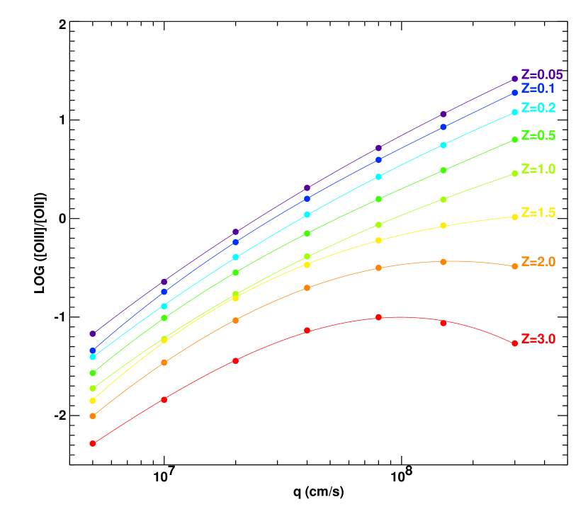
Figure 1: The log([O III] $\lambda 5007/$[O II] $\lambda\lambda 3726,9$) diagnostic versus ionization parameter. Curves for each metallicity between $Z=0.05$ to $3.0$ ${\rm Z}_{\odot}$ are shown. Filled circles represent the data points from our models at ionization parameters from left to right of $5\times 10^{6}$, $1\times 10^{7}$, $2\times 10^{7}$, $4\times 10^{7}$, $8\times 10^{7}$, $1.5\times 10^{8}$, $3\times 10^{8}$ cm/s. This figure is available in color from the on-line version of this article.

Many of the abundance diagnostics commonly used are sensitive to the ionization parameter, and for some ranges of metallicity, they are not useful unless the ionization parameter can be constrained within a small range of possible values. Provided that the EUV spectrum of the exciting source is reasonably well constrained, the ionization parameter is best determined using the ratios of emission-lines of different ionization stages of the same element. In general, the larger the difference in ionization potentials of the two stages, the better the ratio will constrain the ionization parameter. A commonly used ionization parameter diagnostic is based on the ratio of the [O III] $\lambda$5007 and [O II] $\lambda\lambda$3726,9 emission line fluxes; Figure 1.

The smooth curves are third order polynomial fits to the models for each set of metallicities. They have the form:

$$R=k_{0}+k_{1}x+k_{2}x^{2}+k_{3}x^{3}$$ (3)

where $R$ is the flux ratio, in this case, log([O III]/[O II]), $k_{0-3}$ are constants given in Table 2, and $x$ is the ionization parameter of the form $\log(q)$.

It is evident that [O III]/[O II] is not only sensitive to the ionization parameter, but is also strongly dependant on metallicity. An initial guess of metallicity is essential in order to allow a suitable constraint on the ionization parameter. This estimate could then be used in order to then obtain a second, more accurate estimate of the metallicity, and this iterative procedure can be continued until convergence on both parameters is obtained.

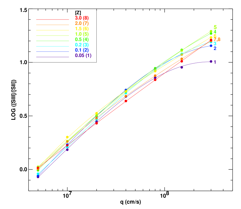
Figure 2: The log([S III] $\lambda\lambda 9069,9532$/ [S II] $\lambda\lambda 6717,31$) diagnostic versus ionization parameter. Curves for each metallicity between $Z=0.05$ to $3.0$ ${\rm Z}_{\odot}$are shown. Filled circles represent the data points from our models at ionization parameters from left to right of $5\times 10^{6}$, $1\times 10^{7}$, $2\times 10^{7}$, $4\times 10^{7}$, $8\times 10^{7}$, $1.5\times 10^{8}$, $3\times 10^{8}$ cm/s. This figure is available in color from the on-line version of this article.

If, however, instead of the oxygen line ratios, one has reliable fluxes for [S III] $\lambda$9069 and/or [S III] $\lambda$9532 as well as the [S II] $\lambda\lambda$6717,31 emission lines, then the [S III]/[S II] ratio provides a rather more useful ionization parameter diagnostic, as shown in Figure 2.

The lack of a strong metallicity dependence in this line ratio is largely due to the fact that the lines used are both in the red portion of the spectrum, and therefore remain strong to much higher metallicities than the [O II] $\lambda\lambda$3726,9 lines. The [O II] $\lambda\lambda$3726,9 lines can only be excited by relatively hot electrons, and so disappear in cooler, high-metallicity H II regions. The lack of a metallicity dependence indicates that the [S III]/[S II] line ratio should make a rather good diagnostic of the ionization parameter. An iterative solution only becomes necessary at the highest values of the [S III]/[S II] ratio; above $\log$([S III]/[S II])$>1.0$.

4 Abundance Sensitive Diagnostic Diagrams

In this section, we present a range of diagnostic diagrams for determining abundance. The choice of the appropriate diagram or combination of diagrams that are to be used by the observer depends on which of the bright emission lines are available. In some cases, an initial guess of metallicity is also useful.

4.1 The [N II]/[O II] Diagnostic Diagram

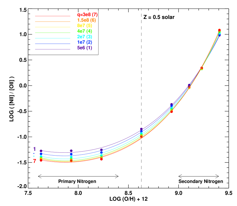
Figure 3: The log([N II] $\lambda 6584$/[O II] $\lambda\lambda 3726,9$) diagnostic for abundance versus metallicity. Curves for each ionization parameter between ${\rm q}=5\times 10^{6}$ to $3\times 10^{8}$ cm/s are shown. Filled circles represent the data points from our models at metallicities from left to right of 0.05, 0.1, 0.2, 0.5, 1.0, 1.5, 2.0, 3.0 ${\rm Z}_{\odot}$. This figure is available in color from the on-line version of this article.

Our calibration of the [N II] $\lambda$6584/[O II] $\lambda$3727 ratio as a function of oxygen abundance is shown in Figure 3 for a set of ionization parameters varying from ${\rm q}=5\times 10^{6}$ to $3\times 10^{8}$ cm/s . The advantages of using the [N II] and [O II] lines are that they are not affected by underlying stellar populations and that they are quite strong, even in low S/N spectra. They do however, need to be corrected for dust extinction.

The curves shown in Figure 3 are fits to the models based on fourth order polynomials of the form:

$$\log(R)=k_{0}+k_{1}x+k_{2}x^{2}+k_{3}x^{3}+k_{4}x^{4}$$ (4)

where $R$ is the flux ratio, in this case, [N II]/[O II], $k_{0-4}$ are constants given in Table 3, and the variable $x$ is the metallicity given in the form $\log({\rm O/H})+12$.

Figure 3 clearly shows that for Z $>$ 0.5 ${\rm Z}_{\odot}$   ($\log({\rm O/H})+12$ $\gtrsim 8.6$), [N II]/[O II] is a very useful diagnostic. Because ${\rm N}^{+}$ and ${\rm O}^{+}$ have similar ionization potentials, this ratio is almost independant of ionization parameter. However, it increases very strongly with metallicity for two reasons. Firstly, [N II] is predominantly a secondary element above metallicities of Z $>$ 0.5 (Alloin et al., 1979; Considère et al., 2000) and consequently the [N II] flux scales more strongly than the [O II] line with increasing metallicity until about 2.0 - 3.0 ${\rm Z}_{\odot}$, when the high metallicity and consequent low electron temperature in the nebula makes both lines very difficult to observe. Secondly, at high metallicity, the lower electron temperature gives fewer thermal electrons of high energy, leading to a strong decrease in the number of collisional excitations of the blue [O II] lines (which has a relatively high threshold energy for excitation) relative to the lower-energy [N II] lines.

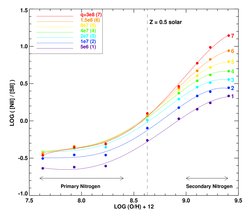
Figure 4: The log([N II] $\lambda 6584$/[S II] $\lambda\lambda 6717,31$) diagnostic for abundance versus metallicity. Curves for each ionization parameter between ${\rm q}=5\times 10^{6}$ to $3\times 10^{8}$ cm/s are shown. Filled circles represent the data points from our models at metallicities from left to right of 0.05, 0.1, 0.2, 0.5, 1.0, 1.5, 2.0, 3.0 ${\rm Z}_{\odot}$. This figure is available in color from the on-line version of this article.

For Z $<$ 0.5 ${\rm Z}_{\odot}$ ($\log({\rm O/H})+12$$<8.6$), the metallicity dependence of the [N II]/[O II] ratio is lost because nitrogen (like oxygen) is predominantly a primary nucleosynthesis element in this metallicity range. In addition, the nitrogen to oxygen abundance ratio shows large scatter from object to object. In this regime, nitrogen production increases as a function of time since the bulk of the star formation occurred (Edmunds & Pagel, 1978; Matteucci & Tosi, 1985; Dopita et al., 1997). Therefore, for a sample of H II regions, the varying age distribution of the stellar population from object to object will cause scatter in the N/O ratios observed. Good evidence for the primary dependence of nitrogen at low abundances can be found in Figure 4 of Considère et al. (2000), in which $\log({\rm N/O})$ derived from a large sample of H II regions is compared with the expected relations for a primary, secondary, and primary + secondary origin for nitrogen production (Vila-Costas & Edmunds, 1993).

We conclude that [N II]/[O II] provides an excellent abundance diagnostic for Z $>$ 0.5 ${\rm Z}_{\odot}$, but this ratio cannot be used at lower abundances.

For Z $>$ 0.5 ${\rm Z}_{\odot}$, the curves in Figure 3 can be fit by a simple quadratic, facilitating abundance determination using the [N II]/[O II] ratio, ie

$$\log({\rm O/H})+12=\log[1.54020+1.26602\,{\rm R}+0.167977\,{\rm R}^{2}]+8.93$$ (5)

where R is $\log($[N II]/[O II]), and $\log({\rm O/H})+12$ must be $\geq 8.6$ for this formula to give a reliable abundance.

Given the large separation in wavelength between the [O II] $\lambda\lambda$3726,9 and [N II] $\lambda$6584 lines, the size and accuracy of determination of the reddening correction remains a concern in the use of this diagnostic. However, we will show in Section 6 that reddening correction using the Balmer decrement and the classical reddening curves provides an adequate accuracy for the use of the [N II]/[O II] ratio in abundance determination. If there was any grounds for concern about the reddening correction used, then a direct measurement of the [O II] $\lambda\lambda$3726,9 to H$\delta$ and [N II] $\lambda$6584 to H$\alpha$ ratios followed by a correction using the theoretical Case B H$\delta$ to H$\alpha$ ratio ($\sim 11$) would provide an adequate reddening correction. An uncorrected reddening of E(B-V) of 0.5 will cause the abundance to be over-estimated by roughly 0.5 dex in $\log({\rm O/H})+12$.

4.2 The [N II]/[S II] Diagnostic Diagram

Our calibration of [N II] $\lambda$6584/[S II] $\lambda\lambda$6717,31 is shown in Figure 4.

As in other diagrams, the smooth curves are fourth order polynomial fits defined as in equation 4, and the coefficients are given in Table 3.

At high metallicity, nitrogen is a secondary nucleosynthesis element and sulphur is a primary $\alpha$-process element. Both lines are close to each other in wavelength, and therefore have similar excitation potentials. At high metallicity, therefore, this line ratio is a function of metallicity thanks primarily to the different nucleogenic status of the two elements. At low metallicity, both the elements are primary and the ratio becomes insensitive to metallicity. This diagnostic is not as useful as [N II]/[O II] for the determination of abundance, but it has the advantage of being far less sensitive to reddening. As [N II]/[S II] is also dependant on ionization parameter, one of the ionization parameter diagnostics should be used in combination with this diagnostic.

4.3 The ${\rm R}_{23}$ Diagnostic Diagram

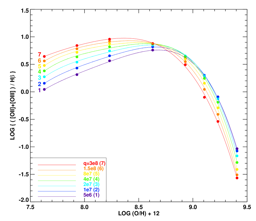
Figure 5: The $\log$(([O II] $\lambda$3727 + [O III] $\lambda\lambda$4959,5007)/H$\beta$) (${\rm R}_{23}$) diagnostic for abundance versus metallicity. Curves for each ionization parameter between ${\rm q}=5\times 10^{6}$ to $3\times 10^{8}$ cm/s are shown. Filled circles represent the data points from our models at metallicities from left to right of 0.05, 0.1, 0.2, 0.5, 1.0, 1.5, 2.0, 3.0 ${\rm Z}_{\odot}$. This figure is available in color from the on-line version of this article.

Since they were first introduced by Pagel et al. (1979), diagnostics based on the so-called ${\rm R}_{23}$ ratio, defined as ${\rm R}_{23}$$=$([O II] $\lambda$3727 + [O III] $\lambda\lambda$4959,5007)/H$\beta$ have found extensive application in the literature. Examples include Alloin et al. (1979); Edmunds & Pagel (1984); McCall, Rybski & Shields (1985); Dopita & Evans (1986); Pilyugin (2000); McGaugh (1991); Pilyugin (2001) and Charlot & Longhetti (2001). As explained in the introduction, ${\rm R}_{23}$ is sensitive to abundance, but is two-valued as a function of metallicity, reaching a maximum at somewhat less than solar abundance (see Figure 5). The smooth curves are fourth order polynomial fits to the models for each ionization parameter defined as in equation 4, with coefficients listed in Table 3 .

Because this ratio is two-valued with metallicity, the key problem associated with the use of this diagnostic to derive abundance is to determine which solution branch applies. This is best determined by the use of an initial guess of the metallicity based on an alternative diagnostic such as [N II]/[O II].

As has been shown in many previous studies, ${\rm R}_{23}$ depends on the ionization parameter, particularly for Z $<0.5$ ${\rm Z}_{\odot}$, but is less sensitive to metallicity in these ranges.

With such a diagnostic, a narrow range of possible ionization parameters can be found using an ionization parameter sensitive ratio such as [O III]/[O II]  and then solving for metallicity. Other methods have used an empirical ‘correction factor’ or ‘excitation parameter’ to correct the observed ${\rm R}_{23}$ for ionization parameter, such as in Pilyugin (2000); Charlot & Longhetti (2001). We prefer to estimate the ionization parameter explicitly, based upon the theoretical models.

4.4 The ${\rm S}_{23}$ Diagnostic Diagram

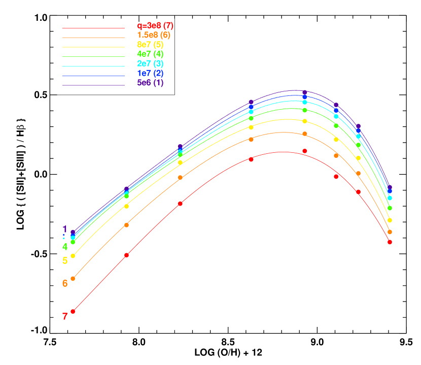
Figure 6: The $\log$(([S II] $\lambda\lambda$6717,31 + [S III] $\lambda\lambda$9069,9532)/H$\beta$) (${\rm S}_{23}$) diagnostic for abundance versus metallicity. Curves for each ionization parameter between ${\rm q}=5\times 10^{6}$ to $3\times 10^{8}$ cm/s are shown. Filled circles represent the data points from our models at metallicities from left to right of 0.05, 0.1, 0.2, 0.5, 1.0, 1.5, 2.0, 3.0 ${\rm Z}_{\odot}$. This figure is available in color from the on-line version of this article.

Our calibration of the ratio ([S II] $\lambda\lambda$6717,31 + [S III] $\lambda\lambda$9069,9532)/H$\beta$ (popularly known as ${\rm S}_{23}$) is shown in Figure 6. Again, we fit fourth order polynomials defined as in equation 4, and the coefficients are given in Table 3.

As is the case in all such ratios of forbidden to recombination lines, the ${\rm S}_{23}$ ratio has a maximum at a certain metallicity, and therefore is two valued at all other metallicities. For this particular ratio the maximum occurs at a somewhat higher abundance than for the ${\rm R}_{23}$ ratio; at metallicities of roughly solar ($\log({\rm O/H})+12$$\sim 8.8$). Again, to raise the degeneracy in the solutions, an initial guess of the metallicity must first be obtained from an alternative diagnostic.

${\rm S}_{23}$ is quite dependant on ionization parameter for all metallicities, and therefore the ionization parameter derived from the [S III]/[S II]  diagnostic should be used to eliminate this as a free variable.

4.5 The [N II]/H$\alpha$ Diagnostic Diagram

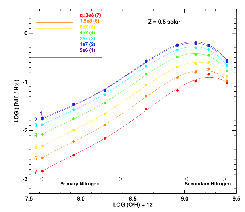
Figure 7: The log([N II] $\lambda 6584$/H$\alpha$) diagnostic for abundance versus metallicity. Curves for each ionization parameter between ${\rm q}=5\times 10^{6}$ to $3\times 10^{8}$ cm/s are shown. Filled circles represent the data points from our models at metallicities from left to right of 0.05, 0.1, 0.2, 0.5, 1.0, 1.5, 2.0, 3.0 ${\rm Z}_{\odot}$. This figure is available in color from the on-line version of this article.

In the absence of other emission lines, the [N II]/H$\alpha$ line ratio can be used as a crude estimator of metallicity. Our calibration of this ratio is shown in Figure 7, with polynomial fits as in equation 4 and coefficients given in Table 3

At very low metallicity, this ratio scales simply as the nitrogen abundance, to first order. However, it is known that in this metallicity regime, the nitrogen abundance shows a lot of scatter relative to the oxygen abundance, since the nitrogen abundance is much more sensitive to the history of star formation in the galaxy considered. As a result, this ratio is probably not very useful to estimate oxygen abundance except as a means of determining the solution branch for the later application of a ratio such as ${\rm R}_{23}$. When the secondary production of nitrogen dominates, at somewhat higher metallicity, the [N II]/H$\alpha$ line ratio continues to increase, despite the decreasing electron temperature. Eventually, at still higher metallicities, nitrogen becomes the dominant coolant in the nebula, and the electron temperature falls sufficiently to ensure that that the nitrogen line weakens with increasing metallicity. Since the [N II] line is produced in the low-excition zone of the H II region, [N II]/H$\alpha$ is also sensitive to ionization parameter.

4.6 The [N II]/[O III] Diagnostic Diagram

The advantage of using [N II] and [O III] lines is that they are unaffected by absorption lines originating from underlying stellar populations, they lie close to Balmer lines that can be used to eliminate errors due to dust reddening, and they are both strong and easily observable in the optical. Both empirical and theoretical relationships for the [N II]/[O III] ratio as a function of oxygen abundance currently exist (eg., Considère et al., 2000).

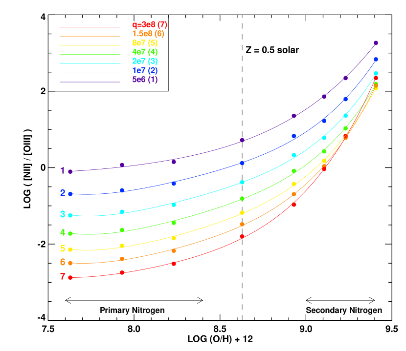
Figure 8: The log([N II] $\lambda 6584$/[O III] $\lambda 5007$ diagnostic for abundance versus metallicity. Curves for each ionization parameter between ${\rm q}=5\times 10^{6}$ to $3\times 10^{8}$ cm/s are shown. Filled circles represent the data points from our models at metallicities from left to right of 0.05, 0.1, 0.2, 0.5, 1.0, 1.5, 2.0, 3.0 ${\rm Z}_{\odot}$. This figure is available in color from the on-line version of this article.

Our calibration of the [N II]/[O III] ratio is shown in Figure 8. The fourth-order polynomial fit coefficients are given in Table 3.

Because the two ions have quite different ionization potentials, the [N II]/[O III] ratio depends strongly on the ionization parameter. Thus, if this diagnostic is to be useful for abundance determinations, it must be used in combination with an independant ionization parameter diagnostic. However, if the [O II] or [S II], and [S III] lines are available to determine the ionization parameter, then it would make more sense to use either the [N II]/[O II] or [N II]/[S II] abundance diagnostics rather than this one.

4.7 Abundance & Ionization Parameter from these Line Ratios

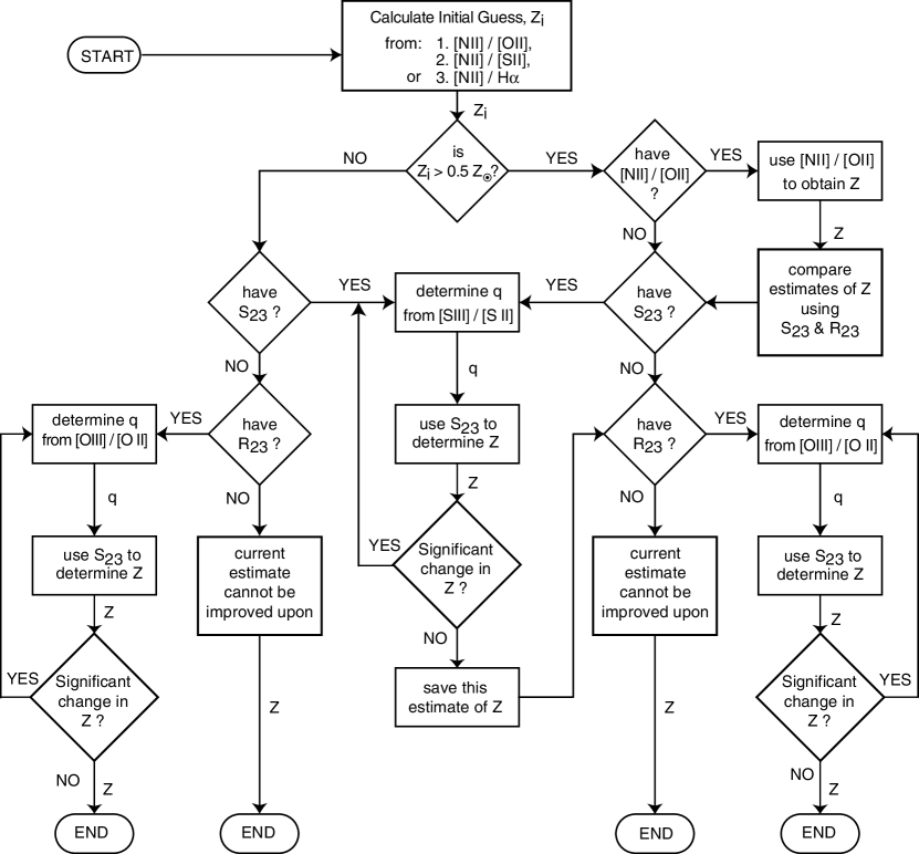
Figure 9: A logical flow diagram for determining abundance and ionization parameter using optical emission-line diagnostics. An IDL script is available from the first author which automatically carries out this process given a set of emission-line fluxes.

Since, in real data sets, we may have available only some of these line ratios, we have summarised in Figure 9 a logical process whereby as many estimates of both the chemical abundance and ionization parameters as are compatible with the data set can be obtained using the techniques described in this section. The process can be automated, and an IDL script to do this is available on request from the first author (LJK). However, we will describe a more direct method for the derivation of these parameters, in Section 7 below. From the comparative analysis with other authors’ techniques which follows, we are confident that this new technique will provide the most reliable abundance estimates currently possible.

5 Comparison with other Bright-Line Techniques

5.1 Comparison Data

Most of the data sets previously used to compare and calibrate abundance diagnostics had been selected in different and heterogeneous ways: some by galaxy (brightest H II regions, or brightest disk H II regions), some by objective prism searches (which are biased towards strong [O III] $\lambda\lambda$49595007), some by Galaxy type (such as dwarf irregulars). These different data sets are reflected in the differences between the various calibrations of abundance. Care must be taken therefore when comparing different abundance diagnostics to take into account biases (if any) introduced by the comparison data.

We chose to use observations of H II regions available from the large and homogeneous data set of van Zee et al. (1998). These authors observed 185 H II regions in 13 spiral galaxies with the Double Spectrograph on the Palomar 5m telescope. These data have the additional advantage of covering a large range in metallicity and ionization parameter, as was shown in Dopita et al. (2000).

Since [S III] measurements are not available for the van Zee H II regions, we have also used two additional data sets for the ${\rm S}_{23}$ diagnostic; Dennefeld & Stasinska (1983) and Kennicutt & Garnett (1996). These also cover a wide range in ionization parameter and metallicity. Using the ESO 3.6m telescope, Dennefeld & Stasinska (1983) observed $\sim 40$ H II regions in the the Magellanic Clouds and the Galaxy, while Kennicutt & Garnett (1996) observed a similar number of H II regions in M101 using the 2.1m telescope at Kitt Peak.

5.2 Comparison Techniques for deriving Abundance

As discussed in the introduction, a wide number of empirical and semi-empirical approaches already exist for the determination of abundances in H II regions. We compare three of the most commonly-used calibrations produced by McGaugh (1991), (hereafter M91), Zaritsky, Kennicutt & Huchra (1994) (hereafter Z94), and Charlot & Longhetti (2001)(herafter C01) with the results produced by our proposed theoretical diagnostics.

M91’s calibration of ${\rm R}_{23}$ makes use of detailed H II region models using the photoionization code CLOUDY (Ferland & Truran, 1981), which also includes the effects of dust and variations in ionization parameter. We have used the analytic expressions for the M91 models given in Kobulnicky, Kennicutt & Pizagno (1999). The Z94 calibration of ${\rm R}_{23}$ for the metal-rich regime is an average of the three calibrations given by Edmunds & Pagel (1984); Dopita & Evans (1986); McCall, Rybski & Shields (1985), with the uncertainty being estimated by the difference between the three determinations. A solution for the ionization parameter is not explicitly included in the Z94 calibration.

C01 gives a number of calibrations depending on the availability of observations of particular spectral lines. Their calibrations are based on a combination of stellar population synthesis and photoionization codes with a simple dust prescription, and include ratios to account for the ionization parameter. As the H II regions in our sample contain measurements of [O III], [O II], [N II]  [S II] and the Balmer lines, we use Case A of C01, which is based on the [N II]/[S II] ratio, with a small dependance on [O III]/[O II] for ionization parameter correction.

Figure 10 shows the oxygen abundances obtained using the Z94, M91 and C01 calibrations for the galaxies in our sample. These clearly show the systematic and random errors associated with each of these calibrations, but it is rather more difficult to estimate the absolute reliability of any particular technique.

The difference between the M91 and Z94 calibrations (Figure 10a) is due to a number of factors. The M91 calibration contains a correction factor based on the ([O III] $\lambda\lambda$49595007/ [O II] $\lambda$3727) ratio in order to account for ionization parameter variations, while the Z94 calibration does not. Z94’s diagnostic was calibrated against a large sample of disk H II regions which span the range $\log({\rm O/H})+12$$>8.35$. As a result, their calibration is only suitable for H II regions in the metal-rich regime, as noted by Kobulnicky, Kennicutt & Pizagno (1999). M91’s diagnostic was calibrated against H II regions from a large range of sources from the literature, including many H II galaxies from the Campbell (1988) objective prism sample, and is parametrized by one polynomial for the metal-poor regime and one for the metal-rich regime.

The C01 calibration when compared with either the Z94 or M91 results shows a large degree of scatter on these diagrams. The C01 calibration (case A) is based on [N II]/[S II]. This ratio is not as sensitive to abundance as ${\rm R}_{23}$, and therefore introduces a large degree of scatter. It is also quite dependant on ionization parameter, which can also increase the scatter. Any technique based on [N II]/[S II] will have a similar amount of scatter, or in other words, a higher uncertainty in the abundance determined. They are therefore not as useful when comparing relative abundances as the techniques with less uncertainty such as ${\rm R}_{23}$ or [N II]/[O II].

The problem of course when comparing abundances derived in this way, is that there is no definitive ‘correct’ answer, since we do not have the [O III] Auroral line as a comparison. In an attempt to overcome this we have taken the average of the abundances derived using all three methods above as a ‘comparison’ abundance. Recalling that the Z94 method is actually based on three previous abundance techniques, this ‘comparison’ abundance is then the average of five virtually independant methods. A single abundance diagnostic will be described below as ‘reliable’ if it can produce the abundances similar to the comparison abundance and also demonstrates a small degree of scatter. The solid line shown in the has the form $y=x$. In the ideal case, with the comparison abundance on one axis and the abundance estimate using a particular technique on the other axis, the data would lie along this solid line. Therefore, the error in an abundance technique can be represented by the root-mean-square distance (rms) of the data to this line. The rms error, given in Table 4, will naturally be increased by both a systematic shift and random scatter, so the rms error should be considered along with the corresponding figure to understand why a particular technique is different to the comparison abundance. Ideally, the rms error should be equal to the rms introduced by uncertainties in the emission-line fluxes measured, which we estimate to be $0.02-0.03$ rms in $\log({\rm O/H})$ for the van Zee data set. Note that an rms error of $\sim 0.1$ or more in $\log({\rm O/H})$ corresponds to an rms error of $>0.5\times$${\rm Z}_{\odot}$ at high abundances (2$\times$${\rm Z}_{\odot}$) and $>0.1\times$${\rm Z}_{\odot}$ at low abundances (0.2$\times$${\rm Z}_{\odot}$). For H II regions or star forming galaxies, this level of accuracy is quite adequate at low abundances, but it may not be sufficient at high abundances. An rms error close to $0.03$ in $\log({\rm O/H})$ ($\sim 0.1\times$${\rm Z}_{\odot}$) would be would be desirable at high abundances. This is especially important in, for example, studies of galactic abundance gradients using H II regions.

First let us see how each of the three comparison techniques; M91, Z94, and C01 compare with the average of all three, shown in Figure 11.

Care must be taken in the interpretation of the panels of Figure 11, since each technique used on the y-axis also contributes to the global average used on the x-axis. This tends to reduce any systematic shift and also decreases the random error. The rms scatter and systematic offsets estimated for any of these techniques are therefore lower limits

With these caveats, it is clear that the M91 method delivers a systematically lower abundance estimate than the average, and becomes quite unreliable for abundances $\log({\rm O/H})+12$$<8.5$. The M91 technique is based on ${\rm R}_{23}$  and as we have already seen, ${\rm R}_{23}$ becomes less sensitive to abundance in this regime. The Z94 method tends to give a higher abundance than the average, and is also not reliable for abundances $\log({\rm O/H})+12$$<8.5$ for the same reason. The observation that M91 and Z94 are not reliable for abundances $\log({\rm O/H})+12$$<8.5$ has also been made by van Zee et al. (1998) who found a similar problem with the ${\rm R}_{23}$ diagnostic of Edmunds & Pagel (1984). The C01 estimates appear to be reliable for all abundances, but is based upon the [N II]/[S II] method, which has a high degree of intrinsic scatter. This scatter is much reduced in this diagram because the C01 abundance estimate is also contributing significantly to the average here. This is verified by Figure 12, which compares the average of M91 and Z94 abundances with those of C01. Since the M91 and Z94 methods are tightly correlated (Figure 10a), the majority of the rms scatter of 0.09 arises with the C01 abundance estimates. Note that since there is no systematic shift observed in this diagram, the average of all three diagnostics should have little or no systematic errors, unless all three are subject to exactly the same form of systematic errors. The latter is a highly unlikely possibility given that all three methods are independantly derived, based on different line ratios, they use different models, and they are calibrated against different data sets. This gives us confidence that, within the scatter, the comparison abundance provides a reliable indicator of the true abundance of a particular H II region or star forming galaxy.

We now proceed to compare our techniques with the average of the comparison techniques. Note that since we have shown that [N II]/H$\alpha$ is relatively insensitive to abundance and is good for an initial guess only, it will not be used further in the analysis.

5.3 The [N II]/[O II] Diagnostic

Our estimate of abundance using [N II]/[O II] (Figure 3) is shown in Figure 13.

Clearly, this provides a very reliable abundance diagnostic. This diagram displays the smallest scatter of any of the techniques presented so far, with an rms error of 0.04. Such a strong correlation between our [N II]/[O II] technique and the average of five previous techniques gives confidence not only in the derived abundance, but also in the reddening correction which has been applied to the observed spectra using the ‘classical’ reddening curves. Clearly, the Balmer decrement has been reliably measured in the H II regions of the van Zee sample.

To better estimate the effect of reddened spectra on the [N II]/[O II] abundance determination, a random reddening corresponding to E(B-V) values between 0 and 1.0 was added to the dereddened fluxes measured in the van Zee H II region spectra. This simulates observations of a sample of H II regions with an average E(B-V) of 0.5.

If we were to then use the [N II]/[O II] diagnostic on this “reddened” sample without correction for reddening, then the abundances estimated are much more scattered, with a systematic shift to higher derived abundances, as shown in Figure 14. The rms error is now 0.14, and a systematic shift of $\log({\rm O/H})+12$ $=0.5$ is observed.

It is clear that, when the Balmer decrement (or another means to estimate E(B-V)) is unavailable, and reddening is believed to be important, the [N II]/[O II] method should not be used.

Note that for large samples of H II regions or starburst galaxies, the tightness of the [N II]/[O II] versus the comparison average may be a good means to test the reliability of the E(B-V) determination. If a shift in this abundance estimate is observed relative to other indicators, then E(B-V) is being systematically underestimated, and if there is a scatter greater than 0.04 rms, then the estimated reddening values should be treated with caution. A random effect such as this might be observed for example in a sample where differing dust geometry affects the reddening of each object in a different fashion.

5.4 The $\mathbf{{\rm R}_{23}}$ Diagnostic

For the ${\rm R}_{23}$ diagnostoc, an initial guess from [N II]/[O II] was used, and the ionization parameter determined using [O III]/[O II]. The abundance was then determined using ${\rm R}_{23}$, with the branch of the ${\rm R}_{23}$ curve chosen depending on whether the initial guess was greater or less than the ${\rm R}_{23}$ maximum ($\log({\rm O/H})+12$ $=8.5$). This process was iterated with [O III]/[O II] until the abundance did not vary. For 88% of the 185 galaxies in the van Zee sample, the abundance converged after 1 iteration. Results for ${\rm R}_{23}$ compared with the average of M91,Z94 and C01 are shown in Figure 15.

Abundances in the region $8.5\leq$$\log({\rm O/H})+12$$\leq 8.9$ cannot be reliably determined due to the maximum in the ${\rm R}_{23}$ versus abundance curve. We see two systematic effects operating in this abundance range. Firstly, there is a systematic shift towards higher estimated abundances than the comparison abundance, which is similar to shifts seen with other ${\rm R}_{23}$ diagnostics (eg. Figure 10a). This is a result of the rapidly declining sensitivity to abundance as the ${\rm R}_{23}$ curve reaches its local maximum at around $\log({\rm O/H})+12$ $=8.5$. The other systematic effect observed is for abundances between 8.5 and 8.8, where the ${\rm R}_{23}$ diagnostic estimates significantly lower abundances between 8.2 and 8.4, causing a branch to appear almost perpendicular to the $y=x$ solid line. This is also a result of the lack of sensitivity of the ${\rm R}_{23}$ diagnostic around its local maximum. If the comparison abundance is correct (and we believe that it is), then these H II regions mostly have an abundance of around $\log({\rm O/H})+12$ $=8.5-8.6$, which is exactly at the local maximum of ${\rm R}_{23}$. An H II region with an abundance of $\log({\rm O/H})+12$ $=8.5-8.6$ will produce ${\rm R}_{23}$ abundance estimates anywhere in the range $\sim 8.8$ or $\sim 8.3$, since this diagnostic is almost insensitive to metallicity throughout this range.

For $\log({\rm O/H})+12$$\geq 8.9$, our ${\rm R}_{23}$ method estimates a somewhat higher abundance estimate than the comparison abundance, but this model-dependent shift is no greater than that seen for other ${\rm R}_{23}$ -based diagnostics (M91 and Z94) in this region. For $\log({\rm O/H})+12$$\leq 8.5$, our ${\rm R}_{23}$ method shows no systematic shift, and gives an rms scatter of 0.07 , which for this abundance range corresponds to an rms of $\sim 0.1\times$${\rm Z}_{\odot}$. This is pleasing, when we consider that some other ${\rm R}_{23}$ techniques fail in this region (Figure 11a,b). The scatter we obtain is similar to that obtained in the C01 [N II]/[S II] method.

5.5 The [N II]/[S II] Diagnostic

Since the [N II]/[S II] diagnostic is primarily sensitive in the high metallicity range and is also sensitive to ionization parameter in this regime, the preferred method is to use an ionization parameter diagnostic such as [O III]/[O II] . However, if [O II] is available, then it would make more sense to use the [N II]/[O II] diagnostic to derive a more reliable abundance, since [N II]/[O II] is much more sensitive to abundance than the [N II]/[S II] ratio. Nevertheless, for completeness, Figure 16 compares the abundance obtained with our [N II]/[S II] method with the average of the three comparison techniques.

Figure 16 shows a large degree of scatter, similar to that seen in the C01 scheme, which is also based on the [N II]/[S II] ratio. This scatter is inherent to using the [N II]/[S II] ratio which is not as sensitive to abundance as other ratios, particularly in the lower metallicity range. In addition, [S II] is affected by the electron density of the line-emitting regions, and this may also contribute towards the scatter. There is also a systematic shift in our estimate of abundance, in the sense that our [N II]/[S II] technique will systematically underestimate the abundance by a factor of $\sim 0.2$ dex compared to the average of the comparison techniques. We believe this is a result either of the use of a different sulfur to oxygen abundance ratio or the depletion factors used in our models for [S II]. Both the large scatter and systematic shift result in a large rms of 0.18 .

The sulfur to oxygen abundance ratio has been found to be the least accurately determined amongst the elements which are usually observed in planetary nebulae (eg. Natta, Panagia & Preite-Martinez, 1980). The determination of the sulfur abundance is particularly difficult because of the large ionization correction factors that must be applied to correct for the presence of unobserved ionization states. These ionization correction factors are often made based on a procedure developed by Peimbert & Costero (1969), which assumes that ions with similar ionization potentials are equally populated. This procedure has been shown to overestimate the S⁺³ abundance by a factor of more than three for most H II regions (Natta, Panagia & Preite-Martinez, 1980). While it is possible to obtain reliable S/O ratios for some low and moderate excitation H II regions (Dennefeld & Stasinska, 1983), it is unreliable for high excitation H II regions (Garnett, 1989). Furthermore, Garnett showed that the [S II]/[S III] ratio is underpredicted by ionization models which produce [O II]/[O III] ratios comparable to observations. Garnett suggests this is a result of uncertainties in model stellar atmosphere fluxes or the atomic data for sulfur. In the light of this discussion, we can probably conclude that the systematic offset that we observe for [N II]/[S II] reflects the systematic errors inherent in any abundance or ionization parameter diagnostic involving sulfur.

5.6 The ${\rm S}_{23}$ Diagnostic

Despite the problems with modeling sulfur as discussed above, and our suspicion that the ${\rm S}_{23}$ diagnostic may not provide a reliable abundance estimate, we have nonetheless applied the ${\rm S}_{23}$ ratio to the H II region data from Dennefeld & Stasinska (1983) and Kennicutt & Garnett (1996) and derived abundances. The ionization parameter was first estimated using the [S III]/[S II] ratio. The ionization parameter obtained with this ratio is compared with that found with the [O III]/[O II] ratio in Figure 17.

This figure shows a large scatter between the two techniques (rms=0.15). Such a scatter in determinining the ionization parameter could introduce an rms scatter in abundance of between 0-0.2 in $\log({\rm O/H})+12$, depending on which diagnostic is used. If the error is concentrated mainly in the [S III]/[S II] ratio, then this alone would be sufficient to cause the large scatter obtained for the [N II]/[S II] diagnostic.

Figure 17 also shows that the [S III]/[S II] ratio gives an ionization parameter which is systematically $\sim 0.2$ dex smaller than that obtained from [O III]/[O II] . This means that all of the H II regions will have an estimated $q<1.5\times 10^{8}$ cm/s, the regime for which the ${\rm S}_{23}$ curve is actually not very sensitive to ionization parameter.

The abundance derived using our ${\rm S}_{23}$ diagnostic is compared with the comparison abundance in Figure 18. Clearly this diagnostic does not reliably estimate abundances for any metallicity range, and should therefore not be used. A reliable theoretical ${\rm S}_{23}$ diagnostic will have to await a resolution of the uncertainties associated with sulfur modeling.

The fact that ${\rm S}_{23}$ underestimates the abundance at low metallicities and overestimates at high metallicities means that the location of the peak of our ${\rm S}_{23}$ grid is too high. Both this and the systematic shift in abundance obtained for the [N II]/[S II] and [S III]/[S II] line ratios can be explained if the sulfur abundance in our models has been under-estimated and that the [S III]/[S II] ratio has been over-estimated. That the [S III]/[S II] ratio has been over-estimated in abundance modelling has been previously suggested by Garnett (1989) as discussed above.

Recently, Diaz & Pérez-Montero (2000) (hereafter DP00) suggested the use of an empirical ${\rm S}_{23}$ diagnostic which they tested using H II regions for which direct determinations for electron temperature were available. These include the Dennefeld & Stasinska (1983) H II regions. The DP00 abundance estimate is compared with the comparison abundance in Figure 19.

The DP00 diagnostic systematically underestimates the abundance relative to the comparison abundance. This underestimation becomes progressively worse at higher metallicity. There is also a very large scatter (rms=0.39). This is probably a result of the linear calibration used by DP00. From Figure 6, it is clear that ${\rm S}_{23}$ can only be fit by a linear calibration up to abundances of about $\log({\rm O/H})+12$$=8.4$, after which the curve begins to turn over. It is interesting that the systematic shift observed here is similar to that found by Kobulnicky, Kennicutt & Pizagno (1999), in that for low metallicity galaxies the [O III] $\lambda$4363 diagnostic systematically underestimated the global oxygen abundance. Nevertheless, in the absence of reliable theoretical ${\rm S}_{23}$ models, empirical calibrations such as that by Diaz & Pérez-Montero (2000) give hope that ${\rm S}_{23}$ can be used as an abundance diagnostic. Indeed, if we add an extra term to the DP00 calibration, such as

$$\log({\rm O/H})+12=1.53\,{\rm S}_{23}+8.27+\frac{1.0}{2.0-9.0\,({\rm S}_{23})^{3}}$$ (6)

(shown in Figure 20), we can produce a correlation between the comparison abundance and the abundance derived above, with a large but significantly reduced rms error of 0.22.

Clearly, more work needs to be done before we can derive a reliable ${\rm S}_{23}$ diagnostic.

6 Optimized abundance determination: Recommended method

As we have seen, with the exception of our [N II]/[O II] diagnostic, all of the comparison techniques and our ${\rm R}_{23}$, [N II]/[S II], and ${\rm S}_{23}$ schemes are plagued by systematic and/or random errors. Nonetheless, some of these techniques, individually or in combination, are reliable over limited ranges of metallicity. It is therefore possible to derive a combined technique which can be used over the entire range of abundances from $\log({\rm O/H})+12$$=8.2$ up to $\log({\rm O/H})+12$$=9.4$. Ideally, this technique will have a small rms, similar to that found with our [N II]/[O II] method, and display no systematic shift relative to the comparison abundance.

The technique presented here applies these criteria, and is applicable to objects for which the spectra include a range of bright emission lines, such as [N II], [O II], [O III], and [S II].

First, we have shown that our [N II]/[O II] diagnostic provides an excellent means of determining abundance for metallicities above $\log({\rm O/H})+12$$=8.6$. For this abundance range, the relationship between the [N II]/[O II] ratio and abundance can be fit by a simple quadratic:

$$\log({\rm O/H})+12=\log[1.54020+1.26602\,{\rm R}+0.167977\,{\rm R}^{2}]+8.93$$ (7)

where R is $\log($[N II]/[O II]). This applies for the high metallicity regime [$\log({\rm O/H})+12\geq 8.6$], and in this regime, the abundance derived from the above equation should be taken as a final abundance estimate. If required, the ionization parameter appropriate to the region observed can then be determined using Figure 1 (equation 3).

Next, if application of the above equation yields an abundance below 8.6, then the average of the M91 and the Z94 methods can be used to provide an abundance estimate. The equation for the Z94 (Zaritsky, Kennicutt & Huchra, 1994) method and the M91 (McGaugh, 1991) method as parametrized by Kobulnicky, Kennicutt & Pizagno (1999) are provided below for reference. Note that Kobulnicky, Kennicutt & Pizagno provided two equations for M91, one for the lower metallicity branch ($\log({\rm O/H})+12$$\leq 8.4$) and one for the upper metallicity branch ($\log({\rm O/H})+12$$>8.4$) The upper branch should be used here, the equation for which is given below.

$${\rm Z94}:\,\log({\rm O/H})+12 = 9.265-0.33\,{\rm R}_{23}-0.202\,{\rm R}_{23}^{2}-0.207\,{\rm R}_{23}^{3}-0.333\,{\rm R}_{23}^{4}$$ (8)

$${\rm M91(u)}:\,\log({\rm O/H})+12 = 12.0-4.944+0.767\,{\rm R}_{23}+0.602\,{\rm R}^{2}_{23}-$$ (9)

$$y\,(0.29+0.332\,{\rm R}_{23}-0.331\,{\rm R}^{2}_{23})$$

where

$$y=\log\left(\frac{[{\rm OIII}]\,\lambda\lambda 4959,5007}{[{\rm OII}]\,\lambda 3727}\right),$$ (10)

unlike the [O III]/[O II] used in our ionization parameter diagnostic or the C01 diagnostic, which are based on the [O III] $\lambda$5007 and [O II] $\lambda$3727 lines only.

The average of these two diagnostics produces reliable abundances down to a $\log({\rm O/H})+12$ of 8.5.

Finally, if this diagnostic gives an estimate below 8.5, then our ${\rm R}_{23}$ method can be used. There is a large degree of scatter inherent at this abundance range for our ${\rm R}_{23}$ method, very similar to that in the C01 method. This scatter is reduced considerably by taking the average of the two techniques. The abundance should first be estimated using the C01 method, as in the following equation, taken from from C01 (Charlot & Longhetti, 2001):

$$\log({\rm O/H})+12=\log\left\{5.09\times 10^{-4}\times\left[\left(\frac{{\rm[OII]/[OIII]}}{1.5}\right)^{0.17}\right]\left[\left(\frac{{\rm[NII]/[SII]}}{0.85}\right)^{1.17}\right]\right\}+12$$ (11)

Note that the line ratios are not used in the logarithmic form for the application of the C01 method, as they are for all the other equations given in this section. This abundance can now be used as an initial guess as input to estimate the ionization parameter to be used in our ${\rm R}_{23}$ method.

For abundances in this regime (below 8.5), the ionization parameter models for $R=\log($[O III]/[O II]) (Figure 1) can be fit by a simple equation of the form:

$$q=10^{({k_{0}+k_{1}*{\rm R}+k_{2}*{\rm R}^{2}})}$$ (12)

where $k_{0-2}$ are constants which depend on the initial guess provided by the C01 method, and are given in Table 2.

Now, with a knowledge of the ionization parameter, we can estimate the abundance using our ${\rm R}_{23}$ method. In this abundance regime the lower branch provides the appropriate solution, given by;

$$\log({\rm O/H})+12=\frac{-k_{1}+\sqrt{k_{1}^{2}-4k_{2}(k_{0}-{\rm R}_{23})}}{2k_{2}}$$ (13)

where $k_{0-2}$ are constants which depend on the ionization parameter derived above, and are given in Table 3.

The solution obtained by the application of this equation can be then substituted in equation 12 to solve again for the the ionization parameter, and the metallicity and the process can be iterated until the solution converges. Generally, we find that convergence is attained after the first iteration in 88% of cases.

The average of our ${\rm R}_{23}$ diagnostic and that given by the C01 method is then adopted for abundances less than $\log({\rm O/H})+12$$=8.5$.

The results of this combined technique is shown against the comparison abundance in Figure 21, and has an rms of 0.05. With the exception of the [N II]/[O II] diagnostic, the combined method outlined above minimizes the scatter inherent in any of the methods presented in this paper, either given by us or by C01, M91, and Z94. In addition, it eliminates the systematic errors which characterize many of the techniques when used alone.

There are four observed points out of 185 which lie off the tight correlation in this figure. These galaxies all have derived abundances based on the [N II]/[O II] ratio which are greater than 8.6, but have comparison abundances between 8.2 and 8.4. We have no reason not to believe our [N II]/[O II] abundance, especially when two of the three comparison abundance diagnostics between 8.2-8.4 (M91 and Z94) are not reliable (eg. Figure 10a,b). Without these four outliers, the rms scatter would reduce still further, to 0.04.

There is a clear gap at abundance $\log({\rm O/H})+12$ $\sim 8.45$. This is a result of the use of ${\rm R}_{23}$ diagnostics, which have a local maximum around this point. Objects which have a real abundance of 8.45 will typically have an abundance estimated from the ${\rm R}_{23}$ ratio of either 8.4 or 8.5, Relative to other errors, this is probably insignificant.

This diagram shows that with this procedure, and providing that we have spectra which include observations of [O II], [N II], [O III], [S II], and, of course, the Balmer lines, it is possible to derive reliable abundances over the whole range of abundances. This procedure utilizes the strengths of various methods, while at the same time minimizes their weaknesses.

7 Solving for Abundances with Limited Data Sets

As we have seen, due to the nature of the diagnostics, the excitation potentials of the lines involved, and their dependance on ionization parameter, different diagnostics are useful over different ranges of metallicity. Most line ratios display a local maximum, causing the metallicity determination to be double valued unless another line ratio can be used to determine on which branch the appropriate solution lies. Others are dependant on ionization parameter over some metallicity ranges, and if these are used, one needs first to solve for the ionization parameter. In many cases, spectra may not cover the full wavelength range needed for the application of the scheme recommended in the previous section. Here we summarize procedures that should provide the most reliable abundance, given such a limited set of emission-line fluxes.

1. [O II], H$\beta$, [O III], [N II], [S II]:

If all of the above lines are available, then our combined method in Section 6 should be used. However, if [N II]/[O II] cannot be corrected for reddening, and the reddening is expected to be significant, then the average of M91, Z94 and C01 will provide reasonable estimate for metallicities above 0.5$\times$solar.

2. [O II], [O III], H$\beta$, [N II]

In the absence of [S II], our combined method can still be used, but for $\log({\rm O/H})+12$ $<8.5$, our ${\rm R}_{23}$ method can be used alone rather than averaging its results with the C01 method. This will increase the rms error in this abundance range to 0.07.

3. [O II], [O III], H$\beta$

If only [O II], [O III], and H$\beta$  are available, then the ${\rm R}_{23}$ diagnostics must be used. Since all the ${\rm R}_{23}$ methods we have looked at contain systematic shifts which apply over particular abundance ranges, the average of the metallicities estimated by a number of ${\rm R}_{23}$ methods is desirable. Since the Z94 ${\rm R}_{23}$ method requires no initial guess, this should be used as an initial guess for both our ${\rm R}_{23}$ method and the M91 method to determine the appropriate solution branch on the ${\rm R}_{23}$ curve. Note that the initial estimate based on Z94 will be very inaccurate at low abundances ($\log({\rm O/H})+12$ $<8.5$), causing metallicities to be over-estimated by a factor of up to 0.5 in $\log({\rm O/H})+12$ in this range. Therefore, in cases where the second $\log({\rm O/H})+12$ estimate (as described below) is lower than the range shown, the abundance should be re-calculated using the method outlined below for the correct abundance range.

We then suggest the application of one of three cases based on this initial guess:

(a) $\log({\rm O/H})+12$ $>9.0$: First find the ionization parameter $q$ from [O III]/[O II] using the Z94 estimate. Next, use this ionization parameter to find which coefficients to use for our ${\rm R}_{23}$ abundance estimate. Estimate $q$ again and check whether it is sufficiently different from the previous estimate of $q$ to influence the abundance derived. Iterate until the abundance estimate converges. Finally, the abundance found with our ${\rm R}_{23}$ method should be averaged with those derived from M91 and Z94.

(b) $8.5<$$\log({\rm O/H})+12$ $\leq 9.0$: The abundances from M91 and Z94 should be averaged to obtain the abundance estimate in this range.

(c) $\log({\rm O/H})+12$ $\leq 8.5$: Our ${\rm R}_{23}$ method alone should be used to determine the abundance, since neither M91 nor Z94 give reliable results in this range. The ionization parameter should be found using [O III]/[O II] and iterated with the abundance as described in (a).

We applied this method to the van Zee H II regions and the results are shown in Figure 22. This method displays an rms scatter of 0.06. Note however, that this is a lower limit because we are using the Z94 and M91 methods for abundances greater than $\log({\rm O/H})+12$ $=8.5$, which also contribute towards the comparison average.

4. [N II], [O II]:

Suppose that only the red [N II] and blue-UV [O II] lines are available. This circumstance might arise, for example, if we are dealing with an intermediate-redshift galaxy ($1.2\leq z\leq 1.7$) in which the [O II] lines are observed in the red, but the H$\alpha$ and [N II] lines are observed in the IR. In this case, the [N II]/[O II] ratio should be used (Figure 3) with equation 4 after correction for reddening. Since this diagnostic is relatively independant of ionization parameter for this metallicity range, no further steps are required to obtain the metallicity. For ${\rm Z}<0.5\,{\rm Z}_{\odot}$ ($\log({\rm O/H})+12$ $\leq 8.6$), [N II]/[O II] is rather insensitive to abundance and the estimate will be affected by a large random error of 0.11 rms.

5. H$\alpha$, [N II], [S II]:

If only red spectra which include H$\alpha$, [N II] and [S II] are available, then the C01 [N II]/[S II] technique cannot be used since it requires a correction factor based on [O III]/[O II] . Our [N II]/[S II] method produces a systematic shift of 0.2 dex. It would be possible therefore to first use the [N II]/[S II] shifted in $\log({\rm O/H})+12$ by 0.2 dex combined with [N II]/H$\alpha$ for an assumed average ionization parameter of $q=2\times 10^{7}~{}cm/s$. Neither of these methods is ideal and both depend strongly on the ionization parameter, which cannot be solved for explicitly, so that this method will only give a very ”rough guess” of the abundance which is probably not useful for detailed abundance studies.

6. [S II], [S III] :

If the sulfur lines are the only ones available, then an empirical abundance diagnostic such as Diaz & Pérez-Montero (2000) as revised here (equation 6) should be used.

8 Conclusions

We have presented a range of diagnostics using current theoretical models for determining the abundances and ionization parameters of star forming regions. The appropriate diagnostics to be used depends on the wavelengths observed, and therefore on the availability of particular emission line ratios. Our diagnostics have been compared with those of McGaugh (1991), Zaritsky, Kennicutt & Huchra (1994) and Charlot & Longhetti (2001), and we arrive at the following conclusions;

1. Our [N II]/[O II] diagnostic is clearly the best diagnostic to use in the Z$>0.5$ ${\rm Z}_{\odot}$ ($\log({\rm O/H})+12$ $>8.6$) regime, as it produces a remarkably tight correlation with the abundance determined using the average of five previous techniques, none of which can reproduce such a tight correlation when used individually. The [N II]/[O II] diagnostic produces this tight correlation as a result of both its independance of ionization parameter and its strong metallicity sensitivity. We have investigated the effect of poorly reddening-corrected or un-corrected spectra on the derived abundance using this diagnostic. We show that this adds both a large degree of uncertainty in the abundance derived, and a systematic bias to estimate higher than average abundances. However, we have shown that ‘classic’ extinction correction methods such as those based on the Whitford reddening curve, provide sufficiently good extinction correction to allow the [N II]/[O II] diagnostic to be used for reliable abundance determinations.

2. As has been shown previously, the common abundance diagnostic ${\rm R}_{23}$ depends strongly on ionization parameter, and the common ionization parameter diagnostic [O III]/[O II] depends strongly on abundance. An iterative approach is often required to resolve these dependancies. Unlike previous methods, we provide techniques for explicitly determining the ionization parameter, rather than including this as a ‘correction factor’ to the abundance diagnostic.

3. Due to the local maximum in ${\rm R}_{23}$, for objects with abundances between $8.4<$ $\log({\rm O/H})+12$ $<8.8$ (ie $0.6<$ log(${\rm R}_{23}$) $<1.0$), a different diagnostic to ours in this range should be used to obtain a more reliable abundance estimate. For $\log({\rm O/H})+12$$\geq 8.9$, our ${\rm R}_{23}$ method delivers a slightly higher abundance than the comparison abundance, but this shift is equal to if not less than that seen for the other two ${\rm R}_{23}$ -based diagnostics (M91 and Z94) in this region. For $\log({\rm O/H})+12$$\leq 8.5$, our ${\rm R}_{23}$ method is much more reliable than the other two ${\rm R}_{23}$ based methods. The C01 [N II]/[S II] method is also reliable in this region, with a similar degree of scatter.

4. We have presented a new combined diagnostic based only on three ${\rm R}_{23}$ diagnostics: ours, M91 and Z94. This diagnostic eliminates the systematic shift inherent to all three techniques used on their own and significantly reduces the scatter or rms error.

5. The ionization parameter diagnostic [S III]/[S II] is independant of abundance, enabling a non-iterative approach to be used if [S III] and [S II] are available in the spectrum. However, our current models do not allow for reliable ionization parameter diagnostics using [S III]/[S II], or abundance determinations derived from ${\rm S}_{23}$. We believe this is a result of either the use of an incorrect sulfur to oxygen abundance ratio, errors in the sulfur depletion factor used, or errors in fundamental atomic data. If the sulfur lines are the only strong lines available, we recommend an empirical method such as that given in Diaz & Pérez-Montero (2000) or the modified Diaz & Pérez-Montero diagnostic presented here which significantly reduces the errors inherent in the Diaz & Pérez-Montero diagnostic alone.

6. Both the [N II]/[S II] and [N II]/H$\alpha$ ratios strongly depend on ionization parameter, so an ionization parameter diagnostic should be used to aid abundance determinations when using these ratios. Neither diagnostic is very sensitive to abundance and should be used with caution. In particular, [N II]/[S II] based diagnostics have a larger degree of uncertainty than schemes based on other ratios such as [N II]/[O II] or ${\rm R}_{23}$.

7. Finally, for spectra of H II regions or star-forming galaxies in which the [N II], [O II], [O III], [S II]  and the Balmer lines of Hydrogen are available, we present a method using a combination of techniques for optimally determining the abundance from these strong lines alone. This method takes advantage of the reliability of our [N II]/[O II] for the intermediate to high metallicity range, and our ${\rm R}_{23}$ diagnostic combined with the Zaritsky, Kennicutt & Huchra (1994), McGaugh (1991) and Charlot & Longhetti (2001) diagnostics for the lower abundance range. This technique can be used over the entire metallicity range, and appears to be prone to much smaller intrinsic errors than all other techniques presented, including those of McGaugh (1991); Zaritsky, Kennicutt & Huchra (1994); Charlot & Longhetti (2001). In addition, there is no systematic offset in the derived abundance when compared with the average of three previous techniques. We strongly recommend use of this technique if all the required emission-lines are available, and fluxes can be extinction corrected using classical methods.

9 Acknowledgements

This work has greatly benefited from discussions with Tim Heckman, Christy Tremonti,Margaret Geller, Rob Kennicutt, Michael Strauss, and Lei Hao. We thank Claus Leitherer and Brigitte Rocca-Volmerange for the use of STARBURST99 and PEGASE 2, and we thank the referee for his comments which made this a more thorough paper. L. Kewley gratefully acknowledges support from the Australian Academy of Science Young Researcher Scheme and from the French Service Culturel & Scientifique. M. Dopita acknowledges the support of the Australian National University and the Australian Research Council through his ARC Australian Federation Fellowship, and under the ARC Discovery project DP0208445.

Figure 10: Oxygen abundance for the van Zee et al. (1998) H II regions using McGaugh (1991) (M91), Zaritsky, Kennicutt & Huchra (1994) (Z94) and Charlot & Longhetti (2001) (C01).

Figure 11: Oxygen abundance for the van Zee et al. (1998) H II regions using McGaugh (1991) (M91), Zaritsky, Kennicutt & Huchra (1994) (Z94) and Charlot & Longhetti (2001) (C01) compared with the average of these three methods (comp - ave).

Figure 12: Oxygen abundance for the van Zee et al. (1998) H II regions found with Charlot & Longhetti (2001) (C01) compared with the average of the abundance from the McGaugh (1991) (M91) and Zaritsky, Kennicutt & Huchra (1994) methods.

Figure 13: Oxygen abundance for the van Zee et al. (1998) H II regions found with our (KD) [N II]/[O II] diagnostic compared with the average (comp - ave) of those found using McGaugh (1991), Zaritsky, Kennicutt & Huchra (1994) and Charlot & Longhetti (2001).

Figure 14: As in Figure 13, but for H II regions with random reddening of $0.0\leq{\rm E(B-V)}\leq 1.0$ added to their spectra.

Figure 15: Oxygen abundance for the van Zee et al. (1998) H II regions found with our (KD) ${\rm R}_{23}$ diagnostic compared with abundances found from the average (comp - ave) of McGaugh (1991), Zaritsky, Kennicutt & Huchra (1994) and Charlot & Longhetti (2001).

Figure 16: Oxygen abundance for the van Zee et al. (1998) H II regions found with our (KD) [N II]/[S II] diagnostic compared with abundances found from the average (comp - ave) of McGaugh (1991), Zaritsky, Kennicutt & Huchra (1994) and Charlot & Longhetti (2001).

Figure 17: Ionization parameter found with our (KD) [S III]/[S II] diagnostic versus ionization parameter found with our [O III]/[O II] diagnostic for the Kennicutt & Garnett (1996) and Dennefeld & Stasinska (1983) H II regions. Ionization parameter is in units of cm/s.

Figure 18: Oxygen abundance for the van Zee et al. (1998) H II regions found with our (KD) ${\rm S}_{23}$ diagnostic compared with abundances found from the average (comp - ave) of McGaugh (1991), Zaritsky, Kennicutt & Huchra (1994) and Charlot & Longhetti (2001).

Figure 19: Oxygen abundance found with the Diaz & Pérez-Montero (2000) (DP00) diagnostic compared with abundances found from the average (comp - ave) of McGaugh (1991), Zaritsky, Kennicutt & Huchra (1994) and Charlot & Longhetti (2001) for the Kennicutt & Garnett (1996) and Dennefeld & Stasinska (1983) H II regions.

Figure 20: Oxygen abundance found with the Diaz & Pérez-Montero (2000) diagnostic with an additional empirical term (DP00/KD) added compared with abundances found from the average (comp - ave) of McGaugh (1991), Zaritsky, Kennicutt & Huchra (1994) and Charlot & Longhetti (2001) for the Kennicutt & Garnett (1996) and Dennefeld & Stasinska (1983) H II regions.

Figure 21: Oxygen abundance for the van Zee et al. (1998) H II regions found with our (KD) combined diagnostic compared with abundances found from the comparison sample which is the average of McGaugh (1991), Zaritsky, Kennicutt & Huchra (1994) and Charlot & Longhetti (2001). This combined technique minimizes the scatter inherent in other techniques and shows no systematic shift compared with the comparison abundance.

Figure 22: Oxygen abundance for the van Zee et al. (1998) H II regions found with our ${\rm R}_{23}$ - only combined diagnostic compared with abundances found from the comparison sample which is the average of McGaugh (1991), Zaritsky, Kennicutt & Huchra (1994) and Charlot & Longhetti (2001). This combined technique minimizes the scatter inherent in other ${\rm R}_{23}$ techniques used alone and shows no systematic shift compared with the comparison abundance.

Table 1: Solar metallicity ($Z_{\odot}$) and depletion factors (D) adopted for each element.

Element	$\log({\rm Z_{\odot}})$	$\log({\rm D})$
H	0.00	0.00
He	-1.01	0.00
C	-3.44	-0.30
N	-3.95	-0.22
O	-3.07	-0.22
Ne	-3.91	0.00
Mg	-4.42	-0.70
Si	-4.45	-1.00
S	-4.79	0.00
Ar	-5.44	0.00
Ca	-5.64	-2.52
Fe	-4.33	-2.00

Table 2: Coefficients for Ionization Parameter Diagnostics

Diagnostic (R)		Z=0.05	0.1	0.2	0.5	1.0	1.5	2.0	3.0 ${\rm Z}_{\odot}$
$\log(\frac{[{\rm OIII}]}{[{\rm OII}]})$	$k_{0}$	-36.9772	-74.2814	-36.7948	-81.1880	-52.6367	-86.8674	-24.4044	49.4728
	$k_{1}$	10.2838	24.6206	10.0581	27.5082	16.0880	28.0455	2.51913	-27.4711
	$k_{2}$	-0.957421	-2.79194	-0.914212	-3.19126	-1.67443	-3.01747	0.452486	4.50304
	$k_{3}$	0.0328614	0.110773	0.0300472	0.128252	0.0608004	0.108311	-0.0491711	-0.232228
$\log(\frac{[{\rm OIII}]}{[{\rm OII}]})$	(Combined method, Section 6)
	$k_{0}$	7.39167	7.46218	7.57817	7.73013	$\cdots$	$\cdots$	$\cdots$	$\cdots$
	$k_{1}$	0.667891	0.685835	0.739315	0.843125	$\cdots$	$\cdots$	$\cdots$	$\cdots$
	$k_{2}$	0.0680367	0.0866086	0.0843640	0.118166	$\cdots$	$\cdots$	$\cdots$	$\cdots$
$\log(\frac{[{\rm SIII}]}{[{\rm SII}]})$	$k_{0}$	30.0116	16.8569	32.2358	-3.06247	-2.94394	-38.1338	-21.0240	-6.61131
	$k_{1}$	-14.8970	-9.62876	-15.2438	-0.864092	-0.546041	13.0914	6.55748	1.36836
	$k_{2}$	2.30577	1.59938	2.27251	0.328467	0.239226	-1.51014	-0.683584	-0.0717560
	$k_{3}$	-0.112314	-0.0804552	-0.106913	-0.0196089	-0.0136716	0.0605926	0.0258690	0.00225792

Table 3: Coefficients for Abundance Diagnostics

Diagnostic (R)		$q=5\times 10^{6}$	$1\times 10^{7}$	$2\times 10^{7}$	$4\times 10^{7}$	$8\times 10^{7}$	$1.5\times 10^{8}$	$3.0\times 10^{8}$
$\log(\frac{[{\rm NII}]}{[{\rm OII}]})$	$k_{0}$	616.294	859.253	1106.87	1307.93	1270.42	1067.21	751.533
	$k_{1}$	-298.819	-413.604	-532.154	-628.828	-612.566	-517.101	-367.682
	$k_{2}$	54.7919	75.1020	96.3733	113.802	111.214	94.4377	67.9579
	$k_{3}$	-4.51877	-6.11475	-7.81061	-9.20734	-9.02939	-7.72256	-5.64034
	$k_{4}$	0.141576	0.188586	0.239282	0.281264	0.276854	0.238784	0.177489
$\log(\frac{[{\rm NII}]}{[{\rm SII}]})$	$k_{0}$	-1042.47	-1879.46	-2027.82	-2080.31	-2162.93	-2368.56	-2910.63
	$k_{1}$	521.076	918.362	988.218	1012.26	1048.97	1141.97	1392.18
	$k_{2}$	-97.1578	-167.764	-180.097	-184.215	-190.260	-205.908	-249.012
	$k_{3}$	8.00058	13.5700	14.5377	14.8502	15.2859	16.4451	19.7280
	$k_{4}$	-0.245356	-0.409872	-0.438345	-0.447182	-0.458717	-0.490553	-0.583763
$\log$(${\rm R}_{23}$)	$k_{0}$	-3267.93	-3727.42	-4282.30	-4745.18	-4516.46	-3509.63	-1550.53
	$k_{1}$	1611.04	1827.45	2090.55	2309.42	2199.09	1718.64	784.26
	$k_{2}$	-298.187	-336.340	-383.039	-421.778	-401.868	-316.057	-149.245
	$k_{3}$	24.5508	27.5367	31.2159	34.2598	32.6686	25.8717	12.6618
	$k_{4}$	-0.758310	-0.845876	-0.954473	-1.04411	-0.996645	-0.795242	-0.403774
$\log$(${\rm S}_{23}$)	$k_{0}$	-1543.68	-1542.15	-1749.48	-1880.06	-1627.10	-1011.65	-81.6519
	$k_{1}$	761.018	758.664	855.280	914.362	790.891	497.017	55.3453
	$k_{2}$	-141.061	-140.351	-157.198	-167.192	-144.699	-92.2429	-13.7783
	$k_{3}$	11.6389	11.5597	12.8626	13.6119	11.7988	7.64915	1.46716
	$k_{4}$	-0.360280	-0.357261	-0.394978	-0.415997	-0.361423	-0.238660	-0.0563760
$\log(\frac{[{\rm NII}]}{{\rm H}\alpha})$	$k_{0}$	-2700.08	-2777.11	-2940.90	-3073.05	-3049.60	-2983.69	-3100.57
	$k_{1}$	1335.14	1369.97	1445.50	1505.94	1491.07	1454.45	1501.77
	$k_{2}$	-247.533	-253.434	-266.482	-276.829	-273.510	-266.015	-272.883
	$k_{3}$	20.3663	20.8100	21.8103	22.5946	22.2767	21.6024	22.0132
	$k_{4}$	-0.62692	-0.63942	-0.6681	-0.6903	-0.6792	-0.6566	-0.6646
$\log(\frac{[{\rm NII}]}{[{\rm OIII}]})$	$k_{0}$	912.833	3720.98	4180.19	4289.18	4209.16	4013.22	3246.13
	$k_{1}$	-461.733	-1792.96	-2011.36	-2064.05	-2032.26	-1950.99	-1604.38
	$k_{2}$	87.8445	324.052	362.929	372.477	367.999	355.774	297.497
	$k_{3}$	-7.45740	-26.0543	-29.1288	-29.9016	-29.6506	-28.8754	-24.5628
	$k_{4}$	0.238581	0.786768	0.877939	0.901534	0.897467	0.880623	0.762337
$\log(\frac{[{\rm NII}]}{[{\rm OII}]})$	(Combined method, Section 6)
	$k_{0}$	1.49089	1.51444	1.54020	1.55753	1.56152	1.55795	1.55354
	$k_{1}$	1.34637	1.31116	1.26602	1.22723	1.20101	1.19010	1.19062
	$k_{2}$	0.204543	0.191521	0.167977	0.145826	0.132789	0.131257	0.139017
$\log$(${\rm R}_{23}$)	(Combined method, Section 6)
	$k_{0}$	-27.0004	-31.2133	-36.0239	-40.9994	-44.7026	-46.1589	-45.6075
	$k_{1}$	6.03910	7.15810	8.44804	9.78396	10.8052	11.2557	11.2074
	$k_{2}$	-0.327006	-0.399343	-0.483762	-0.571551	-0.640113	-0.672731	-0.674460

Table 4: RMS Error measured from the solid $x=y$ line shown on the Figures given in column 1.

Figure	X-axis	Y-axis	RMS Error	Comments
10a	M91	Z94	0.18	strong systematic shift, tight correlation at high abundances
10b	M91	C01	0.11	large degree of scatter, systematic shift
10c	C01	Z94	0.13	large degree of scatter, small systematic shift
11a	Comp. Ave	M91	$>0.09$	M91 contributes to both axes, systematic shift.
11b	Comp. Ave	Z94	$>0.10$	M91 contributes to both axes, systematic shift.
11c	Comp. Ave	C01	$>0.06$	C01 contributes strongly to both axes
12	M91,Z94 Ave	C01	0.09	no systematic shift
13	Comp. Ave	KD - [NII]/[OII]	0.04	no systematic shift.
14	Comp. Ave	KD - [NII]/[OII] reddened	0.14	systematic shift, large degree of scatter
15	Comp. Ave	KD - ${\rm R}_{23}$	0.14	systematic shift, large scatter at low abundances.
16	Comp. Ave	KD - [NII]/[SII]	0.18	strong systematic shift and scatter.
17	KD - [SIII]/[SII]	KD - [OIII]/[OII]	0.25	strong scatter & systematic shift
18	Comp. Ave	KD - ${\rm S}_{23}$	0.32	strong systematic shift and scatter
19	Comp. Ave	DP00 ${\rm S}_{23}$	0.44	large scatter, systematic shift
20	Comp. Ave	DP00/KD ${\rm S}_{23}$	0.25	smaller scatter than DP00, but still significant
21	Comp. Ave	KD - combination scheme	0.05	no systematic shift, 4 outliers (rms is 0.04 without outliers)
22	Comp. Ave	${\rm R}_{23}$ only combined scheme	$>0.06$	no systematic shift

References

- Allende Prieto, Lambert, & Asplund (2001) Allende Prieto, C., Lambert, D. L., & Asplund, M. 2001, ApJ, 556, 63
- Aller (1942) Aller, L. H. 1942, ApJ, 95, 52
- Aller (1990) Aller, L. H. 1990, PASP, 102, 1097
- Alloin et al. (1979) Alloin, D., Collin-Souffrin, S., Joly, M. & Vigroux, L. 1979, A&A, 78, 200
- Anders & Grevesse (1989) Anders, E. & Grevesse, N. 1989, Geochim. & Cosmochim. Acta 53, 197
- Campbell (1988) Campbell, A. 1988, ApJ, 335, 644
- Charlot & Longhetti (2001) Charlot, S. & Longhetti, M. 2001, MNRAS, 323, 887
- Considère et al. (2000) Considère, S., Coziol, R., Contini, T. & Davoust, E. 2000, A&A, 356, 89
- Dennefeld & Stasinska (1983) Dennefeld, M. & Stasinska, G. 1983, A&A, 118, 234
- Diaz & Pérez-Montero (2000) Diaz, A. I. & Pérez-Montero 2000, MNRAS, 312, 130
- Dopita & Evans (1986) Dopita, M.A. & Evans, I.N. 1986, ApJ, 307, 431
- Dopita et al. (2000) Dopita, M. A., Kewley, L. J., Heisler, C. A., & Sutherland, R. S. 2000, ApJ, 542,224
- Dopita & Sutherland (1996) Dopita, M. A., & Sutherland, R. 1996, ApJS, 102, 161
- Dopita & Sutherland (2000) Dopita, M. A. & Sutherland, R. S. 2000 ApJ, 539, 742
- Dopita et al. (1997) Dopita, M. A, Vassiliadis, E., Wood, P. R., Meatheringham, S. J., Harrington, J. P., Bohlin, R. C., Ford, H. C., Stecher, T. P., & Maran, S. P. 1997, ApJ, 474, 188
- Edmunds & Pagel (1984) Edmunds, M.G. & Pagel, B.E.J. 1984, MNRAS, 211, 507
- Edmunds & Pagel (1978) Edmunds, M. G. & Pagel B. E. J., 1978, MNRAS, 185, 77P
- Ferland & Truran (1981) Ferland, G. J. & Truran, J. W. 1981, ApJ, 244, 1022
- Ferland et al. (1998) Ferland, G. J., Korista, K. T., Verner, D. A., Ferguson, J. W., Kingdon, J. B., & Verner, E. M. 1998, PASP, 110, 761
- Fioc & Rocca-Volmerange (1997) Fioc, M., & Rocca-Volmerange, B. 1997, A&A, 326, 950
- Garnett (1989) Garnett, D. 1989, ApJ, 345, 282
- Kennicutt & Garnett (1996) Kennicutt, R. C. & Garnett, D. R. 1996, ApJ, 456, 504
- Kewley et al. (2001) Kewley, L. J., Dopita, M. A., Sutherland, R. S., Heisler, C. A. & Trevena, J. 2001, ApJ, 556, 121
- Kobulnicky & Zaritsky (1999) Kobulnicky, H. A., & Zaritsky, D. 1999, ApJ, 511, 120.
- Kobulnicky, Kennicutt & Pizagno (1999) Kobulnicky, H. A., Kennicutt, R. C., & Pizagno, J. L. 1999, ApJ, 514, 544
- Leitherer et al. (1999) Leitherer, C., Schaerer, D., Goldader, J. D., Delgado, R. M. González, R. C., Kune, D. F., de Mello, Duília F., Devost, D., & Heckman, T. M. 1999, ApJS, 123, 3
- Mas-Hesse & Kunth (1991) Mas-Hesse, J. M. & Kunth, D. 1991, A&AS, 88, 399
- Mathis, Rumpl & Nordsieck (1977) Mathis, J.S., Rumpl, W. & Nordsieck, K.H. 1977, ApJ, 217, 425
- Matteucci & Tosi (1985) Matteucci, F. & Tosi, M. 1985, MNRAS, 217, 391
- McCall, Rybski & Shields (1985) McCall, M.L., Rybski, P.M. & Shields, G.A. 1985, ApJS, 57, 1
- McGaugh (1991) McGaugh, S.S. 1991, ApJ, 380, 140
- Natta, Panagia & Preite-Martinez (1980) Natta, A., Panagia, N., & Preite-Martinez, A. 1980, ApJ, 242, 596
- Osterbrock (1989) Osterbrock, D. E. 1989, Astrophysics of Gaseous Nebulae and Actuve Galactic Nuclei (Mill Valley; University Science Books)
- Pagel et al. (1979) Pagel, B. E. J. et al 1979, MNRAS, 189, 95
- Pagel, Edmunds & Smith (1980) Pagel, B. E. J., Edmunds, M. G., & Smith, G. 1980, MNRAS, 193, 219
- Pagel (1986) Pagel, B. E. J. 1986, PASP, 98, 1009
- Peimbert & Costero (1969) Peimbert, M. & Costero, R. 1969, Bol. Obs. Tonantzintla y Tacubaya, 5, 3
- Peimbert (1975) Peimbert, M., Rayo, J. F., Torres-Peimbert, S. 1975, RMxAA, 1, 289
- Pilyugin (2000) Pilyugin, L. S. 2000, A&A, 362, 325
- Pilyugin (2001) Pilyugin, L. S. 2001, A&A, 369, 594
- Russell & Dopita (1992) Russell, S. C. & Dopita, M.A. 1992, ApJ, 384, 508
- Shields (1990) Shields, J. C. 1990, ARA&A, 28, 525
- Skillman, Kennicutt & Hodge (1989) Skillman, E. D., Kennicutt, R. C., & Hodge, P. W. 1989, ApJ, 347, 875
- Steidel et al. (1996) Steidel, C. C., Giavalisco, M., Pettini, M., Dickinson, M., & Adelberger, K. L. 1996, ApJ, 462, 17
- Sutherland & Dopita (1993) Sutherland, R.S. & Dopita, M.A. 1993, ApJS, 88, 253
- Thurston, Edmunds, & Henry (1996) Thurston, T. R., Edmunds, M. G. & Henry, R. B. C. 1996, MNRAS, 283, 990
- Torres-Peimbert, Peimbert & Fierro (1989) Torres-Peimbert, S., Peimbert, M., & Fierro, J. 1989, ApJ, 345, 186
- van Zee et al. (1998) van Zee, L. et al. 1998, AJ, 116, 2805
- van Zee, Haynes & Salzer (1997) van Zee, L. Haynes, M.P. & Salzer, J.J. 1997, in IAU Symp. 187: “Cosmical Chemical Evolution”, 49
- Vila-Costas & Edmunds (1993) Vila-Costas, M. B., Edmunds, M. B. 1993, MNRAS, 265, 199
- Zaritsky, Kennicutt & Huchra (1994) Zaritsky, D., Kennicutt, R. C., & Huchra, J. P. 1994, ApJ, 420, 87