Cosmological Acceleration Through Transition
to Constant Scalar Curvature

Abstract

As shown by Parker and Raval, quantum field theory in curved spacetime gives a possible mechanism for explaining the observed recent acceleration of the universe. This mechanism, which differs in its dynamics from quintessence models, causes the universe to make a transition to an accelerating expansion in which the scalar curvature, $R$, of spacetime remains constant. This transition occurs despite the fact that we set the renormalized cosmological constant to zero. We show that this model agrees very well with the current observed type-Ia supernova (SNe-Ia) data. There are no free parameters in this fit, as the relevant observables are determined independently by means of the current cosmic microwave background radiation (CMBR) data. We also give the predicted curves for number count tests and for the ratio, $w(z)$, of the dark energy pressure to its density, as well as for $dw(z)/dz$ versus $w(z)$. These curves differ significantly from those obtained from a cosmological constant, and will be tested by planned future observations.

1 Introduction

Observational evidence appears increasingly strong that the expansion of the universe is undergoing acceleration that started at a redshift $z$ of order 1 (Riess et al., 1998, 2001; Perlmutter et al., 1998, 1999). Observations of scores of type-Ia supernovae (SNe-Ia) out to $z$ of about 1.7 support this view (Riess et al., 2001), and even glimpse the earlier decelerating stage of the expansion. It is fair to say that one of the most important questions in physics is: what causes this acceleration?

One of the more obvious possible answers is that we are observing the effects of a small positive cosmological constant $\Lambda$ (Krauss & Turner, 1995; Ostriker & Steinhardt, 1995; Dodelson, Gates, & Turner, 1996; Colberg et al., 2000). Another, less obvious possibility is that there is a quintessence field responsible for the acceleration of the universe (Caldwell, Dave, & Steinhardt, 1998; Zlatev, Wang, & Steinhardt, 1999; Dodelson, Kaplinghat, & Stewart, 2000; Armendariz-Picon, Mukhanov, & Steinhardt, 2001). Quintessence fields are scalar fields with potential energy functions that produce an acceleration of the universe when the gravitational and classical scalar (quintessence) field equations are solved. More recently, Parker & Raval (1999a, b, c, 2000, 2001) showed that a quantized free scalar field of very small mass in its vacuum state may accelerate the universe. Their model differs from any quintessence model in that the scalar field is free, thus interacting only with the gravitational field. The nontrivial dynamics of this model arises from well-defined finite quantum corrections to the action that appear only in curved spacetime. This was the first model to present a realization of dark energy with ratio of pressure to energy density taking values more negative than $-1$. Other models having this property have subsequently been proposed (Caldwell, 2002; Melchiorri et al., 2002).

The physics of the Parker-Raval model is based on quantum field theory in curved spacetime. The renormalized (i.e., observed) cosmological constant $\Lambda$ is set to zero. Several mechanisms have been proposed that tend to drive the value of $\Lambda$ to zero (Dolgov, 1983; Ford, 1987, 2002; Tsamis & Woodard, 1998a, b; Abramo, Tsamis, & Woodard, 1999), but these mechanisms play no role in this model. The energy-momentum tensor of the quantized field in its vacuum state is determined by calculating an effective action (Schwinger, 1951; DeWitt, 1965; Jackiw, 1974) in a general curved spacetime. The spacetime is unquantized, and is itself determined self-consistently from the Einstein gravitational field equations involving the vacuum expectation value of the energy-momentum tensor, as well as the classical energy momentum tensor of matter (including cold dark matter) and radiation. In solving the Einstein equations, the symmetries of the FRW spacetime are imposed, but the spacetime is not otherwise taken as fixed, and the initial value constraints of general relativity are satisfied. The acceleration is the result of including in the effective action a non-perturbative term involving the scalar curvature of the spacetime (Parker & Toms, 1985a, b, c; Jack & Parker, 1985). The minimal effective action that includes this non-perturbative effect and gives the correct trace anomaly of the energy-momentum tensor was used by Parker and Raval. In applying this effective action to the recent expansion of the universe, terms involving more than two derivatives of the metric were neglected. In this approximation, a solution was proposed in which the universe undergoes a rapid transition from a standard FRW universe dominated by cold dark matter to one containing significant contributions of vacuum energy and pressure. The proposal is that this negative vacuum pressure is responsible for the observed acceleration of the universe. The reaction back of this negative vacuum pressure on the expansion of the universe is such as to cause a rapid transition to an expansion of the universe in which the scalar curvature remains constant. The vacuum pressure and energy density are determined by a single parameter related to the mass of the scalar field. The transition to constant scalar curvature is the result of a rapid growth in the magnitudes of the vacuum pressure and energy density that occurs in this theory when the scalar curvature approaches a particular value, of the order of the square of the mass of the particle associated with the scalar field. The Einstein equations cause a reaction back on the metric such as to prevent further increase in the magnitudes of the vacuum pressure and energy density. (This effect is analogous to Lenz’s law in electromagnetism.)

The essential cosmological features of this model may be described quite simply. For times earlier than a time $t_{j}$ (corresponding to $z\sim 1$), the universe undergoes the stages of the standard model, including early inflation, and radiation domination followed by domination by cold dark matter. During the latter stage, at time $t_{j}$ the vacuum energy and (negative) pressure of the free scalar quantized field increase rapidly in magnitude (from a cosmological point of view). The effect of this vacuum energy and pressure is to cause the scalar curvature $R$ of the spacetime to become constant at a value $R_{j}$. The spacetime line element is that of an FRW universe:

$$ds^{2}=-dt^{2}+a(t)^{2}[(1-kr^{2})^{-1}dr^{2}+r^{2}d\theta^{2}+r^{2}\sin^{2}{\theta}d\phi^{2}]\;,$$ (1)

where $k={\pm 1}$ or $0$ indicates the spatial curvature. By joining at $t_{j}$ the matter dominated scale parameter $a(t)$ and its first and second derivatives to the solution for $a(t)$ in a constant $R$ universe, one uniquely determines the scale parameter $a(t)$ for times after $t_{j}$. This model is known as the vacuum cold dark matter (VCDM) model of Parker and Raval, or as the vacuum metamorphosis model (Parker & Raval, 1999c) to emphasize the existence of a rapid transition in the vacuum energy density and pressure.

The constant value, $R_{j}$, of the scalar curvature is a function of a single new parameter, $\bar{m}$, related to the mass of the free scalar field. Therefore, the function $a(t)$ for $t>t_{j}$ is fully determined by $\bar{m}$. The values of $\bar{m}$ and $t_{j}$ can be expressed in terms of observables, namely, the present Hubble constant $H_{0}$, the densities $\Omega_{m0}$ and $\Omega_{r0}$ of the matter and radiation, respectively, relative to the closure density, and the curvature parameter $\Omega_{k0}\equiv-k/(H_{0}^{2}a_{0}^{2})$. (Here $a_{0}\equiv a(t_{0})$ is the present value of the cosmological scale parameter.) These observables have been determined with reasonably good precision by various measurements that are independent of the SNe-Ia (Krauss, 2000; Freedman et al., 2001; Hu et al., 2001; Huterer & Turner, 2001; Turner, 2001; Wang, Tegmark, & Zaldarriaga, 2002). Therefore, the value of $\bar{m}$ is known to within narrow bounds, independently of the SNe-Ia observations.

The power spectrum of the CMBR depends largely on physical processes occurring long before $t_{j}$. The behavior of $a(t)$ in the VCDM model does not significantly differ from that of the standard model until after $t_{j}$. Therefore, the predicted power spectrum in the VCDM model differs only slightly from that of the standard model. We calculate the predicted power spectrum of the CMBR in the VCDM model (as described below), and find the range of values of the above observables that give a good fit to the CMBR observations.

From this range of observables, the corresponding range of the parameter $\bar{m}$ follows. Therefore, the prediction of the VCDM model for the magnitude versus redshift curve of the SNe-Ia is completely determined, with no adjustable parameters. We plot the predicted curves (obtained from this range of $\bar{m}$) for the distance modulus $\Delta(m-M)$ of the SNe-Ia as a function of $z$. Comparison with the observed data points, as summarized by Riess et al. (2001), shows that a significant subset of predicted curves fit the SNe-Ia data very well, passing within the narrow error bars of each of the binned data points, as well as of the single data point at $z\approx 1.7$.

We also give the curves predicted by the VCDM model for number counts of cosmological objects as a function of $z$ and for the ratio, $w(z)$, of the vacuum pressure to vacuum energy density, as well as for $dw/dz$ versus $w$ (parametrized by $z$). The predictions of the VCDM model differ significantly from those of the $\Lambda$CDM model. Accurate measurements of these quantities out to $z$ of about 2 would be very telling.

The model we consider here is the simplest of a class of models in which a transition occurs around a finite value of $z$ within the range of possible observation. This general class has been studied from a phenomenological point of view by Bassett et al. (2002a, b). They find that the CMBR, large scale structure, and supernova data tend to favor a late-time transition over the standard $\Lambda$CDM model. Although they considered only dark-energy equations of state, $w$, with $w>-1$, their phenomenological analysis can be generalized to include the present VCDM model. In addition, the VCDM model is readily generalized to include a nonzero vacuum expectation value of the low mass scalar field, which could bring $w$ into the range greater than $-1$. In the present paper, we are taking the simplest of the possible VCDM (or vacuum metamorphosis) models, so as to introduce no arbitrary parameters into the fit to the supernova data.

2 How Observables Determine $\bar{m}$

In this section, we explain how the value of $\bar{m}$ is obtained from $H_{0}$, $\Omega_{k0}$, $\Omega_{m0}$, and $\Omega_{r0}$ in the VCDM model. (Here, $\Omega_{m0}\equiv\Omega_{{\rm cdm}0}+\Omega_{b0}$, where $\Omega_{{\rm cdm}0}$ and $\Omega_{b0}$ are the present densities of cold dark matter and baryons, respectively, relative to the closure density.) The relation between $\bar{m}$ and these present observables follows from the Einstein equations, the previously described constancy of the scalar curvature $R=R_{j}$ for $t>t_{j}$, and continuity of $a(t)$ and its first and second derivatives at time $t_{j}$. For our present purposes, we may define the parameter $\bar{m}$ in terms of $R_{j}$, namely, by the relation $\bar{m}^{2}=R_{j}$. (At a microscopic level, $\bar{m}$ is proportional to the mass of the free quantized scalar field.)

The trace of the Einstein equations at time $t_{j}$ is

$$\bar{m}^{2}=R_{j}=8\pi G\rho_{mj}\;,$$ (2)

where $\rho_{mj}$ is the energy density of the non-relativistic matter present at time $t_{j}$. The density and pressure of the dark energy, $\rho_{v}$ and $p_{v}$, respectively, will be taken to be zero at $t_{j}$. We make this assumption in order to avoid introducing a second parameter in addition to $\bar{m}$. It should be noted for future reference that dropping this assumption will introduce another parameter that would affect mainly the behavior of the predicted SNe-Ia curve near the transition time $t_{j}$ from matter-dominated to constant-scalar-curvature universe. In the present paper, we do not relax this assumption of zero $\rho_{vj}$ and $p_{vj}$ because we find good agreement of the one parameter VCDM model with the current observational data.

For all $t>t_{j}$, the scalar curvature is taken to remain constant at the value $R_{j}=\bar{m}^{2}$. Thus,

$$6[(\dot{a}/a)^{2}+(\ddot{a}/a)+k/a^{2}]=\bar{m}^{2}\;,$$ (3)

where dots represent time derivatives. Defining the variable $x\equiv a^{2}$, this becomes

$$\frac{1}{2}\ddot{x}+k=\frac{1}{6}\bar{m}^{2}x\;.$$ (4)

The first integral of this equation is

$$\frac{1}{4}\dot{x}^{2}-\frac{1}{12}\bar{m}^{2}x^{2}+kx=E\;,$$ (5)

where $E$ is a constant.

One of the Einstein equations at time $t_{j}$ is

$$H_{j}^{2}+k/a_{j}^{2}=(8\pi G/3)\rho_{j}\;,$$ (6)

where $H_{j}\equiv{\dot{a}}(t_{j})/a(t_{j})$, $a_{j}\equiv a(t_{j})$, and $\rho_{j}\equiv\rho(t_{j})$ is the total energy density at time $t=t_{j}$. The last equation can be rewritten as

$$\frac{1}{4}\dot{x}_{j}^{2}+kx_{j}=(8\pi G/3)\rho_{j}x_{j}^{2}\;,$$ (7)

where subscript $j$ refers to quantities at time $t_{j}$. Comparing this with equation (5), one finds that

$$E=\left[(8\pi G/3)\rho_{j}-\frac{1}{12}\bar{m}^{2}\right]x_{j}^{2}\;.$$ (8)

Using $\rho_{j}=\rho_{mj}+\rho_{rj}$, where $\rho_{rj}$ is the radiation energy density at time $t_{j}$, and equation (2) to eliminate $\rho_{j}$ and $\rho_{mj}$ from the last expression for $E$, we find that

$$E=(8\pi G/3)\rho_{rj}x_{j}^{2}+\frac{1}{4}\bar{m}^{2}x_{j}^{2}\;.$$ (9)

Thus, equation (5) gives the following conserved quantity:

$$\frac{1}{4}\dot{x}^{2}-\frac{1}{12}\bar{m}^{2}x^{2}+kx=(8\pi G/3)\rho_{rj}x_{j}^{2}+\frac{1}{4}\bar{m}^{2}x_{j}^{2}\;.$$ (10)

This is readily written in terms of $a(t)$ and its derivatives. We have $\dot{x}/x=2\dot{a}/a\equiv 2H(t)$, and $x_{j}^{2}/x(t)^{2}=[a_{j}/a(t)]^{4}$. Hence, the radiation energy density satisfies

$$\rho_{rj}x_{j}^{2}/x(t)^{2}=\rho_{r}(t)\;,$$ (11)

and equation (10) is

$$H(t)^{2}+k/a(t)^{2}=(8\pi G/3)\rho_{r}(t)+\frac{1}{4}\bar{m}^{2}[a_{j}/a(t)]^{4}+\frac{1}{12}\bar{m}^{2}\;.$$ (12)

Solving for $[a_{j}/a(t)]^{4}$, we obtain (for $t\geq t_{j}$),

$$[a_{j}/a(t)]^{4}=\frac{4}{\bar{m}^{2}}\left[H(t)^{2}+k/a(t)^{2}-(8\pi G/3)\rho_{r}(t)\right]-\frac{1}{3}\;.$$ (13)

Returning to equation (2), we can now express $\bar{m}$ in terms of the present values of $\rho_{m}$, $\rho_{r}$, $H$, and $k/a$. We have

$$\bar{m}^{2}=R_{j}=8\pi G\rho_{m0}(a_{0}/a_{j})^{3}\;.$$ (14)

With equation (13), it follows that

$$\bar{m}^{2}=8\pi G\rho_{m0}\left\{\frac{4}{\bar{m}^{2}}\left[H_{0}^{2}+k/a_{0}^{2}-(8\pi G/3)\rho_{r0}\right]-\frac{1}{3}\right\}^{-3/4}.$$ (15)

Using the expression for the present critical density, $\rho_{c0}=3H_{0}^{2}/(8\pi G)$, equation (15) takes the dimensionless form,

$${m_{H0}}^{2}=3\Omega_{m0}\left\{(4/m_{H0}^{2})\left[1-\Omega_{k0}-\Omega_{r0}\right]-\frac{1}{3}\right\}^{-3/4},$$ (16)

where $m_{H0}\equiv\bar{m}/H_{0}$. This is readily solved numerically for $m_{H0}^{2}$. Alternatively, it can be put into the form of a fourth-order equation for $m_{H0}^{2}$ and solved analytically. Using the values $\Omega_{m0}=0.34^{+0.46}_{-0.14}$ and $H_{0}=65^{-16}_{+10}$ ${\rm km}~{}{\rm s}^{-1}~{}{\rm Mpc}^{-1}$ obtained in section 5 from the CMBR power spectrum (see fig. 2), as well as $\Omega_{r0}=8.33\times 10^{-5}$ and $\Omega_{k0}=0$, we find $m_{H0}=3.26^{-0.62}_{+0.10}$ and $\bar{m}=4.5^{-1.7}_{+0.9}\times 10^{-33}\;\;{\rm eV}$. (The uncertainties refer to the $95\%$ confidence level.) Note that the fitting of the CMBR power spectrum alone gives us a wide range for $\Omega_{m0}$ and $H_{0}$. In order to further restrict our results (thus being able to make stronger predictions), we will adopt the HST-Key-Project result $H_{0}=72\pm 8$ ${\rm km}~{}{\rm s}^{-1}~{}{\rm Mpc}^{-1}$ (Freedman et al., 2001) as a constraint. This narrows the range of our cosmological parameters down to $\Omega_{m0}=0.34^{+0.08}_{-0.14}$ and $H_{0}=65^{-1}_{+10}$ ${\rm km}~{}{\rm s}^{-1}~{}{\rm Mpc}^{-1}$, as can be seen from figure 2. Aiming at combining these two methods of determining the uncertainties of our results, hereafter we adopt the notation exemplified by $\Omega_{m0}=0.34^{+(0.46;0.08)}_{-0.14}$ and $H_{0}=65^{-(16;1)}_{+10}$ ${\rm km}~{}{\rm s}^{-1}~{}{\rm Mpc}^{-1}$, where the uncertainties appearing in parenthesis refer to the $95\%$ confidence level, without and with the HST constraint, respectively. (The sign appearing in front of the parenthesis is common to both uncertainties.) Thus, returning to the parameters $m_{H0}$ and $\bar{m}$, we have:

$$m_{H0}=3.26^{-(0.62;0.08)}_{+0.10}\;$$ (17)

and

$$\bar{m}=4.52^{-(1.76;0.18)}_{+0.84}\times 10^{-33}\;\;{\rm eV}\;.$$ (18)

Finally, the solution to equation (4) for $x(t)=a(t)^{2}$ is

$$a(t)^{2}/a_{0}^{2} = \cosh\left(\frac{\bar{m}}{\sqrt{3}}(t-t_{0})\right)$$ (19)

$$+\frac{2\sqrt{3}}{m_{H0}}\sinh\left(\frac{\bar{m}}{\sqrt{3}}(t-t_{0})\right)$$

$$-\frac{6\Omega_{k0}}{m_{H0}^{2}}\cosh\left(\frac{\bar{m}}{\sqrt{3}}(t-t_{0})\right)+\frac{6\Omega_{k0}}{m_{H0}^{2}}\;.$$

It then follows from $(1/2)\dot{x}(t)/x(t)=H(t)$, that

$$H(t)/H_{0} = a(t)^{-2}a_{0}^{2}\left[\cosh\left(\frac{\bar{m}}{\sqrt{3}}(t-t_{0})\right)\right.$$ (20)

$$\left.+\sqrt{3}\left(\frac{m_{H0}}{6}-\frac{\Omega_{k0}}{m_{H0}}\right)\sinh\left(\frac{\bar{m}}{\sqrt{3}}(t-t_{0})\right)\right]\;.$$

From equations (12), (14), and (16) one obtains the following expression in terms of the redshift, $z\equiv a_{0}/a-1$:

$$H(z)^{2}/H_{0}^{2}=(1-\Omega_{k0}-m_{H0}^{2}/12)(1+z)^{4}+\Omega_{k0}(1+z)^{2}+m_{H0}^{2}/12\;.$$ (21)

From equations (14) and (17) one finds the redshift $z_{j}$ at time $t_{j}$,

$$z_{j}=[m_{H0}^{2}/(3\Omega_{m0})]^{1/3}-1=1.19^{-(0.76;0.19)}_{+0.47}\;.$$ (22)

Moreover, from equation (21) we can obtain the redshift, $z_{a}$, at which the expansion of the Universe starts to accelerate. In fact, by looking at the deceleration parameter,

$$q\equiv-\frac{a\ddot{a}}{\dot{a}^{2}}=(1+z)\left[\ln\left(H/H_{0}\right)\right]^{\prime}-1\;,$$ (23)

where the prime sign stands for derivative with respect to $z$, we have that $z_{a}$ satisfies

$$(1+z_{a})H^{\prime}(z_{a})=H(z_{a})\;.$$ (24)

Thus, from equation (21) and the cosmological parameters mentioned above, we obtain for the spatially flat VCDM model

$$z_{a}=\left[\frac{m_{H0}^{2}/12}{1-\Omega_{k0}-m_{H0}^{2}/12}\right]^{1/4}-1=0.67^{-(0.59;0.15)}_{+0.35}\;.$$ (25)

This value is similar to the one obtained using the spatially flat $\Lambda$CDM model with $\Omega_{\Lambda 0}=0.67$:

$$z_{a\Lambda{\rm CDM}}\approx\left(\frac{2\Omega_{\Lambda 0}}{1-\Omega_{\Lambda 0}}\right)^{1/3}-1\approx 0.60\;.$$ (26)

3 The Dark Energy

In the VCDM model, the dark energy is the energy of the vacuum, denoted by $\rho_{v}$. This vacuum energy is not in the form of real particles, but may be thought of as energy associated with fluctuations (or virtual particles) of the quantized scalar field. Vacuum energy, $\rho_{v}$, and pressure, $p_{v}$, must be included as a source of gravitation in the Einstein equations. Thus, for $t>t_{j}$, one has

$$H(t)^{2}+k/a(t)^{2}=(8\pi G/3)\left[\rho_{r}(t)+\rho_{m}(t)+\rho_{v}(t)\right]\;.$$ (27)

The vacuum energy and pressure remain essentially zero until the time $t_{j}$ when the value of the scalar curvature $R$ has fallen to a value slightly greater than $\bar{m}^{2}$. Then in a short time (on a cosmological scale), the vacuum energy and pressure grow, and through their reaction back cause the scalar curvature to remain essentially constant at a value just above $R_{j}=\bar{m}^{2}$ (Parker & Raval, 1999a, b). Intuitively, this reaction back may be thought of as similar to what happens in electromagnetism when a bar magnet is pushed into a coil of wire. The current induced in the coil produces a magnetic field that opposes the motion of the bar magnet into the coil (Lenz’s Law). Similarly, in the present case, the matter dominated expansion of the universe causes the scalar curvature to decrease. But as it approaches the critical value, $\bar{m}^{2}$, the quantum contributions to the energy-momentum tensor of the scalar field grow large in such a way as to oppose the decrease in $R$ that is responsible for the growth in quantum contributions. The universe continues to expand, but in such a way as to keep $R$ from decreasing further.

Defining $t_{j}$ as the time at which $\rho_{v}$ and $p_{v}$ begin to grow significantly, we have to good approximation, equation (2). Evolving $\rho_{m_{j}}$ forward in time, then gives

$$8\pi G\rho_{m}(t)=\bar{m}^{2}\left[a_{j}/a(t)\right]^{3}.$$ (28)

One then finds from equation (27) and equation (12) that the vacuum energy density evolves for $t>t_{j}$ as

$$\rho_{v}(t)=\frac{\bar{m}^{2}}{32\pi G}\left\{1-4\left[a_{j}/a(t)\right]^{3}+3\left[a_{j}/a(t)\right]^{4}\right\}\;.$$ (29)

The conservation laws for the total energy density and pressure and for the energy densities and pressures of the radiation alone and of the matter alone, then imply that $\rho_{v}$ and the vacuum pressure, $p_{v}$, also satisfy the conservation law. It follows that

$$p_{v}(t) = -\frac{d}{dt}(\rho_{v}a^{3})/\frac{d}{dt}(a^{3})$$ (30)

$$= \frac{\bar{m}^{2}}{32\pi G}\left\{-1+\left[a_{j}/a(t)\right]^{4}\right\}\;.$$

At late times, as $a_{j}/a(t)$ approaches zero, one sees that the vacuum energy density and pressure approach those of a cosmological constant, $\Lambda=\bar{m}^{2}/4$. But at finite times, their time evolution differs from that of a cosmological constant.

One immediately sees from equations (28) and (29) that for $t>t_{j}$,

$$\rho_{v}(t)+\rho_{m}(t)=\frac{\bar{m}^{2}}{32\pi G}\left\{1+3\left[a_{j}/a(t)\right]^{4}\right\}\;.$$ (31)

Using equation (30), it now follows that

$$p_{v}(t)=(1/3)\left[\rho_{v}(t)+\rho_{m}(t)\right]-\bar{m}^{2}/(24\pi G)\;.$$ (32)

Since $p_{m}=0$, and $p_{r}=(1/3)\rho_{r}$, the total pressure, $p$, and energy density, $\rho$, satisfy the equation of state (Parker & Raval, 2000)

$$p(t)=(1/3)\rho(t)-\bar{m}^{2}/(24\pi G)\;.$$ (33)

From this equation of state and the conservation law, which can be written in the form, $d(\rho a^{3})/da+pd(a^{3})/da=0$, we find that for $t>t_{j}$,

$$\rho(a)=\left(\rho_{j}-\frac{\bar{m}^{2}}{32\pi G}\right)(a_{j}/a)^{4}+\frac{\bar{m}^{2}}{32\pi G}\;.$$ (34)

As the vacuum energy density is taken as zero at $t=t_{j}$, we have $\rho_{j}=\rho_{mj}+\rho_{rj}=\rho_{m0}a_{0}^{3}/a_{j}^{3}+\rho_{r0}a_{0}^{4}/a_{j}^{4}$, and then, from equation (14),

$$\rho_{j}=\bar{m}^{2}/(8\pi G)+\rho_{r0}\left[\bar{m}^{2}/(8\pi G\rho_{m0})\right]^{4/3}.$$ (35)

Then, with equation (28) and (for $t>t_{j}$) $(a_{j}/a)^{4}=(a_{0}/a)^{4}(8\pi G\rho_{m0}/\bar{m}^{2})^{4/3}$, equation (34) finally becomes

$$\rho(a)=\left[\rho_{m0}\,(3\Omega_{m0}/m_{H0}^{2})^{1/3}+\rho_{r0}\right]\,(a_{0}/a)^{4}+\bar{m}^{2}/(32\pi G)\;.$$ (36)

This expression will be used in the next section to calculate, among other things, the age of the Universe as predicted by the VCDM model.

4 Age of the universe

The values of $t_{j}$ and $t_{0}$ are found by integration:

$$t=\int_{0}^{t}\,dt=\int_{0}^{a(t)}\,da\,a^{-1}H(a)^{-1}.$$ (37)

From equation (27),

$$t=\int_{0}^{a(t)}\,da\,a^{-1}\,\left\{-k/a^{2}+(8\pi G/3)\left[\rho_{r}(a)+\rho_{m}(a)+\rho_{v}(a)\right]\right\}^{-1/2},$$ (38)

This integral is conveniently split in two at time $t_{j}$, and expressed in terms of variable of integration $y\equiv a/a_{0}$:

$$t_{j}=(H_{0})^{-1}\int_{0}^{a_{j}/a_{0}}\,dy\,\left(\Omega_{k0}+\Omega_{m0}y^{-1}+\Omega_{r0}y^{-2}\right)^{-1/2},$$ (39)

and from equation (36),

$$t_{0}-t_{j}=(H_{0})^{-1}\int_{a_{j}/a_{0}}^{1}\,dy\,\left\{\Omega_{k0}+\left[\Omega_{m0}\,(3\Omega_{m0}/m_{H0}^{2})^{1/3}+\Omega_{r0}\right]\,y^{-2}+(m_{H0}^{2}/12)\,y^{2}\right\}^{-1/2}.$$ (40)

Another interesting parameter to obtain is $t_{a}$, the time when the expansion of the Universe starts to accelerate:

$$t_{0}-t_{a}=(H_{0})^{-1}\int_{a_{a}/a_{0}}^{1}\,dy\,\left\{\Omega_{k0}+\left[\Omega_{m0}\,(3\Omega_{m0}/m_{H0}^{2})^{1/3}+\Omega_{r0}\right]\,y^{-2}+(m_{H0}^{2}/12)\,y^{2}\right\}^{-1/2},$$ (41)

where $a_{a}\equiv a(t_{a})$.

Using the cosmological parameters obtained in section 5 by fitting the VCDM model to the CMBR power spectrum data, we have (see eqs. [22] and [25]) $a_{j}/a_{0}=(1+z_{j})^{-1}=0.46^{+(0.24;0.04)}_{-0.08}$  and  $a_{a}/a_{0}=(1+z_{a})^{-1}=0.60^{+(0.32;0.06)}_{-0.10}$,  and  consequently,  $H_{0}t_{j}=0.354^{+(0.084;0.009)}_{-0.011}$, $H_{0}t_{a}=0.535^{+(0.126;0.013)}_{-0.017}$, and $H_{0}t_{0}=0.99^{-(0.26;0.07)}_{+0.16}$. Thus, using the correspondent values of $H_{0}$, we finally obtain

$$t_{j}=5.33^{+(3.41;0.22)}_{-0.84}\;{\rm Gyr}\;,$$ (42)

$$t_{a}=8.0^{+(5.2;0.4)}_{-1.2}\;{\rm Gyr}\;,$$ (43)

and

$$t_{0}=14.9\mp 0.8\;{\rm Gyr}\;.$$ (44)

Note that the uncertainty in $t_{0}$ is independent of whether or not we adopt the HST-Key-Project result as a constraint. This is because the dependence of $t_{0}$ on $H_{0}$ and $\Omega_{m0}$ is such that the $95\%$ confidence region shown in figure 2 happens to be stretched along lines of constant values of $t_{0}$. The same is true for the $\Lambda$CDM model, as discussed by Knox, Christensen, & Skordis (2001).

We can compare the values presented in equations (43) and (44) with the respective ones given by the spatially flat $\Lambda$CDM model. Using $\Omega_{\Lambda 0}=0.67$, the $\Lambda$CDM model gives $H_{0}t_{a}\approx 0.536$ and $H_{0}t_{0}\approx 0.938$. With the best-fit value of the Hubble constant obtained for our model, $H_{0}=65$ ${\rm km}~{}{\rm s}^{-1}~{}{\rm Mpc}^{-1}$ (see section 5), this gives $t_{a}\approx 8.1\;{\rm Gyr}$ and $t_{0}\approx 14.1\;{\rm Gyr}$. Therefore, we see that the age attributed to the Universe by the VCDM model is larger than the age predicted by the $\Lambda$CDM model, for essentially the same values of $\Omega_{m0}$ and $H_{0}$.

5 Fit to the CMBR power spectrum

In view of recent CMBR observations (Pryke et al., 2002; Masi et al., 2002; Netterfield et al., 2002; Abroe et al., 2001), there is a need to reexamine the results obtained by Parker & Raval (2001). In this section, we will obtain the cosmological parameters $\omega_{{\rm cdm}0}\equiv\Omega_{{\rm cdm}0}h^{2}$, $\omega_{b0}\equiv\Omega_{b0}h^{2}$, and $H_{0}\equiv 100h$ ${\rm km}~{}{\rm s}^{-1}~{}{\rm Mpc}^{-1}$ which give the best fit of the spatially flat VCDM model to the recent measurements of the CMBR power spectrum by Boomerang, MAXIMA, and DASI ($h$ is a dimensionless quantity defined by the latter expression). As we have seen, these parameters are the essential ingredients necessary to fix the parameter $\bar{m}$. [The other necessary parameter, $\Omega_{r0}=8.33\times 10^{-5}$, is independently obtained from the CMBR mean temperature and the number of relic neutrino species (Peebles, 1993).]

In order to obtain the CMBR power spectrum fluctuations predicted by the VCDM model, with given values of $\omega_{{\rm cdm}0}$, $\omega_{b0}$, and $H_{0}$, we use a slightly modified version of the CMBFAST computer code (Seljak & Zaldarriaga, 1996; Zaldarriaga & Seljak, 2000). The modifications made in the code, described by Parker & Raval (2001), consist of adding the vacuum contributions, $\rho_{v}$ and $p_{v}$, to the total energy density and pressure, respectively, for time $t>t_{j}$, i.e., after the transition to dark energy dominated epoch.

We set up the CMBFAST code to generate a numerical grid in the 3 dimensional cosmological parameter space ($\omega_{{\rm cdm}0}$, $\omega_{{\rm b}0}$, $H_{0}$). We introduce prior information on the value of the present day Hubble constant, $H_{0}$, to be in the range from 45 to 80 with units of km Mpc^-1 s^-1. Also, we set the value of the cosmological constant, $\Lambda$, to be zero. To perform our numerical analysis consistent with these priors, we generated a class of VCDM models with the following cosmological parameters and resolutions (in the form of “initial value”:“final value”:“step size”): $\omega_{b0}=(0.005:0.030:0.001)$, $\omega_{{\rm cdm}0}=(0.05:0.31:0.01)$, and $H_{0}=(45.0:80.0:1.0)$ ${\rm km}~{}{\rm s}^{-1}~{}{\rm Mpc}^{-1}$. We chose to vary these three parameters based on the fact that they determine directly $\bar{m}$, which is the one free parameter of the VCDM model. All models generated use the Radical Compression Data Analysis Package (RadPack) (Bond, Jaffe, & Knox, 2000) to compute a $\chi^{2}$ test statistic that compares the predicted CMBR spectrum to the experimental measurements of DASI (Pryke et al., 2002), Boomerang (Masi et al., 2002; Netterfield et al., 2002), and MAXIMA (Abroe et al., 2001) at particular multipoles $l$. We look for minima of $\chi^{2}$ in the class of cosmologies specified above. The particular VCDM model described by the parameters which give the minimum of $\chi^{2}$ in our parameter space is called the best fit model.

Table 1: Multipole numbers $l$ and associated power intensities $I_{l}$ of the first few peaks and troughs of the CMBR spectrum predicted by the spatially flat VCDM model (see fig. 1). The uncertainties $\Delta l$ and $\Delta I_{l}$ are calculated from the $\chi^{2}$ test statistic.

	$l$	$\Delta l$	$I_{l}\;(\mu{\rm K}^{2})$	$\Delta I_{l}\;(\mu{\rm K}^{2})$
Peaks	$230$	$\pm 1$	$5133$	$+22$/$-337$
	$558$	$+7$/$-5$	$2436$	$+162$/$-123$
	$848$	$+4$/$-9$	$2441$	$+291$/$-229$
Troughs	$427$	$+2$/$-7$	$1591$	$+132$/$-81$
	$700$	$+7$/$-20$	$1685$	$+173$/$-158$

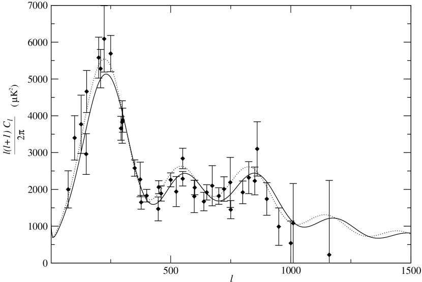
Figure 1: Plot of the best fit CMBR power spectrum for the spatially flat VCDM model (solid curve) and of the CMBR power spectrum for the spatially flat $\Lambda$CDM model with $\Omega_{\Lambda 0}=0.67$ (dashed curve). The diamond points and error bars correspond to DASI, Boomerang, and MAXIMA experimental data.

For the best fit VCDM model, we found $\omega_{b0}=0.022$, $\omega_{{\rm cdm}0}=0.12$, and $H_{0}=65.0$ ${\rm km}$ ${\rm s}^{-1}$ ${\rm Mpc}^{-1}$. This best fit has $\chi^{2}=\chi_{min}^{2}=48.84$, corresponding to a significance level $\alpha(\chi_{min})\equiv\int_{\chi_{min}^{2}}^{\infty}f(\chi^{2},n)\;d(\chi^{2})=0.187$, where $f(\chi^{2},n)=\left[2\Gamma(n/2)\right]^{-1}(\chi^{2}/2)^{n/2-1}e^{-\chi^{2}/2}$ is the $\chi^{2}$ probability density function (pdf) for $n$ degrees of freedom (the recent CMBR data we consider are constituted of $41$ experimental points). The three best fit cosmological parameters of the VCDM model are similar to the values obtained from the $\Lambda$CDM model fit to the CMBR power spectrum (Pryke et al., 2002; Abroe et al., 2001; Masi et al., 2002; Netterfield et al., 2002).

To find the 95$\%$ confidence region of our parameter space, we compute the quantity $\chi_{95\%}^{2}$ where $\alpha(\chi_{95\%})=0.05$, and then look for the subset of VCDM models with $\chi^{2}\leq\chi^{2}_{95\%}$ which lie in the parameter space given above. The results for the VCDM model are $H_{0}=65_{+10}^{-16}$ ${\rm km}~{}{\rm s}^{-1}~{}{\rm Mpc}^{-1}$, $\omega_{{\rm cdm}0}=0.12^{+0.06}_{-0.03}$, and $\omega_{b0}=0.022^{+0.003}_{-0.004}$. The uncertainties given above are obtained from the extrema of the 95$\%$ confidence region. The range of $\omega_{b0}$ is consistent with Big Bang Nucleosynthesis (Bean, Hansen, & Melchiorri, 2002), and the best fit value for $H_{0}$ lies within the range given by the HST Key Project (Freedman et al., 2001).

From the $95\%$ confidence region in the parameter space ($\omega_{{\rm cdm}0}$, $\omega_{b0}$, $H_{0}$) we can obtain the $95\%$ confidence region in the space ($\Omega_{m0}$, $H_{0}$), recalling that $\Omega_{m0}=(\omega_{{\rm cdm}0}+\omega_{b0})/h^{2}$ and $h\equiv H_{0}/\left(100\;{\rm km}\;{\rm s}^{-1}\;{\rm Mpc}^{-1}\right)$. This confidence region is presented in figure 2 (dark-gray region). The reason to concentrate in the parameter space ($\Omega_{m0}$, $H_{0}$) is that all quantities we are interested in (e.g., the age of the Universe, the luminosity distances of SNe-Ia, number count tests, the dark energy equation of state) depend directly on $\Omega_{m0}$, not on $\omega_{{\rm cdm}0}$ and $\omega_{b0}$ separately (except, obviously, the quantities directly related to the CMBR power spectrum). From figure 2 we see that $\Omega_{m0}=0.34^{+0.46}_{-0.14}$. This very wide range is just a consequence of the fact that the Hubble constant $H_{0}$ is not tightly constrained by the CMBR power spectrum. However, adopting the HST-Key-Project result $H_{0}=72\pm 8$ ${\rm km}~{}{\rm s}^{-1}~{}{\rm Mpc}^{-1}$ as a constraint (light-gray region in fig. 2), the acceptable range of $\Omega_{m0}$ can be narrowed down to $\Omega_{m0}=0.34^{+0.08}_{-0.14}$, which then allows us to make stronger predictions about the cosmological quantities mentioned above. Using the even stronger prior $H_{0}=65$ ${\rm km}~{}{\rm s}^{-1}~{}{\rm Mpc}^{-1}$ (the best-fit value) we obtain the “best-fit range” $\Omega_{m0}=0.34\pm 0.06$, which will be used in the next section to fit (with no free parameters) the luminosity distances of SNe-Ia.

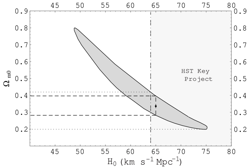
Figure 2: Plot of the $95\%$ confidence level (dark-gray region) in the parameters $\Omega_{m0}$ and $H_{0}$ obtained by fitting the CMBR power spectrum using the VCDM model. The extrema of this region, together with the best-fit values, define the ranges $\Omega_{m0}=0.34^{+0.46}_{-0.14}$ and $H_{0}=65^{-16}_{+10}$ ${\rm km}~{}{\rm s}^{-1}~{}{\rm Mpc}^{-1}$. Adopting the HST-Key-Project result ($H_{0}=72\pm 8$ ${\rm km}~{}{\rm s}^{-1}~{}{\rm Mpc}^{-1}$, represented by the light-gray region), the range in $\Omega_{m0}$ is narrowed down to $\Omega_{m0}=0.34^{+0.08}_{-0.14}$ (dotted lines). Fixing $H_{0}=65$ ${\rm km}~{}{\rm s}^{-1}~{}{\rm Mpc}^{-1}$, we have $\Omega_{m0}=0.34\pm 0.06$ (dashed lines).

For the CMBR power spectrum predicted by the best fit flat VCDM model (see fig. 1), the multipole numbers $l$ and power intensities $I_{l}\equiv l(l+1)C_{l}/(2\pi)$ of the first three peaks and two troughs are given in table 1. The uncertainties $\Delta l$ and $\Delta I_{l}$ correspond to the 95% confidence region of $\omega_{{\rm cdm}0}$, $\omega_{b0}$, and $H_{0}$. Comparing the values given in table 1 with the correspondent results presented by Durrer, Novosyadlyj, & Apunevych (2001), we see that our values for the first three peaks and two troughs are well within the ($1\sigma$) ranges for these quantities that can be obtained, in a model-independent way, from the combined Boomerang, MAXIMA, and DASI data. For instance, the last two columns of table 2 of Durrer, Novosyadlyj, & Apunevych (2001) give the multipole number and the power intensity of the first peak to be $l_{p_{1}}=213^{+35}_{-59}$ and $I_{p_{1}}=5041^{+1017}_{-1196}$ $\mu$K², respectively.

The results of this section show that the VCDM model gives a reasonable fit to the CMBR power spectrum with values of $\omega_{{\rm cdm}0}$, $\omega_{b0}$, and $H_{0}$ that are consistent with current observations. The future of CMBR observations looks very promising with a mixture of ground based interferometers (DASI), airborne interferometers (MAXIMA and Boomerang), and satellite experiments (Microwave Anisotropy Probe and the Planck satellite) that will further probe the CMBR anisotropies at higher and lower multipoles.

6 No-parameter fit to the SNe-Ia data

In the present section we compare the luminosity distance as a function of redshift predicted by the VCDM model to the measured values of the luminosity distances of SNe-Ia as summarized by Riess et al. (2001). Because all the relevant parameters of the model are determined by fitting the CMBR power spectrum (see sec. 5), this comparison is a no-parameter fit of the VCDM model to the SNe-Ia data.

We start by computing the luminosity distance as a function of redshift, $d_{L}(z)$. As a consequence of equation (1), the comoving coordinate distance $r(z)$ of objects observed with redshift $z$ satisfies

$$\frac{dr}{\sqrt{1-kr^{2}}}=\frac{dt}{a(t)}=\frac{dz}{a_{0}H(z)}\;,$$ (45)

which leads to

$$r(z)=\cases{\int_{0}^{z}\left[a_{0}H(z^{\prime})\right]^{-1}dz^{\prime}&, $k=0$\cr\left(a_{0}H_{0}\Omega_{k0}^{1/2}\right)^{-1}\sinh\left(H_{0}\Omega_{k0}^{1/2}\int_{0}^{z}H(z^{\prime})^{-1}dz^{\prime}\right)&, $k\neq 0$},$$ (46)

where $H(z)$ for the VCDM model is given by (see eq. [21])

$$\frac{H(z)}{H_{0}}=\cases{\left[\left(1-\Omega_{k0}-m_{H0}^{2}/12\right)\left(1+z\right)^{4}+\Omega_{k0}\left(1+z\right)^{2}+m_{H0}^{2}/12\right]^{1/2}&, $z<z_{j}$\cr\left[\Omega_{r0}\left(1+z\right)^{4}+\Omega_{m0}\left(1+z\right)^{3}+\Omega_{k0}\left(1+z\right)^{2}\right]^{1/2}&, $z\geq z_{j}$}.$$ (47)

The luminosity distance and the distance modulus are defined respectively as

$$d_{L}(z)\equiv a_{0}\left(1+z\right)r(z)$$ (48)

and

$$\Delta\left(m-M\right)(z)\equiv 5\log\left(\frac{d_{L1}(z)}{d_{L2}(z)}\right),$$ (49)

where $d_{L1}$ is the luminosity distance in the spatially flat VCDM model and $d_{L2}$ is the luminosity distance in an arbitrary fiducial model used as normalization. We will set $d_{L2}$ as the luminosity distance in an open and empty Universe [$a(t)=t$ and $k=-1$], which is the convention used by Riess et al. (2001).

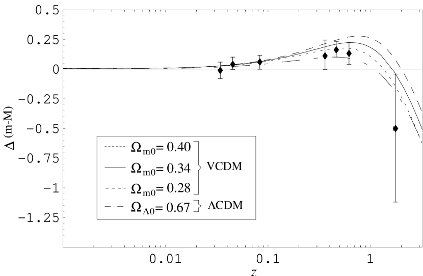
Figure 3: Plot of the type-Ia supernovae distance modulus (normalized to a spatially open and empty cosmos) as a function of redshift $z$ for the spatially flat VCDM (with $\Omega_{m0}=0.34\pm 0.06$) and $\Lambda$CDM (with $\Omega_{\Lambda 0}=0.67$) models.

It is important to note that the expression for $\Delta\left(m-M\right)$ does not depend explicitly on the present value of the Hubble constant $H_{0}$. However, if we adopt the results of the previous section summarized in figure 2, then fixing different values of $H_{0}$ in that figure lead to different $95\%$-confidence-level ranges for $\Omega_{m0}$, which in turn give rise to different predictions for the SNe-Ia luminosity distances. In particular, using for $H_{0}$ the best-fit value $H_{0}=65$ ${\rm km}~{}{\rm s}^{-1}~{}{\rm Mpc}^{-1}$ gives us $\Omega_{m0}=0.34\pm 0.06$ (see fig. 2). In figure 3 we plot the distance modulus as a function of redshift predicted by the VCDM model using this “best-fit range” for $\Omega_{m0}$, as well as the observed distance moduli of SNe-Ia. It can be seen from figure 3 that fixing the values of $\Omega_{m0}$ and $H_{0}$ that best fit the CMBR data also gives a very good no-parameter fit to the SNe-Ia data. Moreover, any value of $\Omega_{m0}$ in the “best-fit range” $\Omega_{m0}=0.34\pm 0.06$ gives a reasonably good fit to the SNe-Ia data, as shown by the dashed curves in figure 3. We also show in figure 3 the distance modulus predicted by the $\Lambda$CDM model with $\Omega_{\Lambda 0}=0.67$. We see that even though the predictions of both models differ significantly in the range $0.5\lesssim z\lesssim 1.5$, current data are still not able to make a clear distinction between them.

More numerous and accurate data on SNe-Ia luminosity distance are expected for the near future. The planned Supernova Acceleration Probe (SNAP), for instance, aims at cataloging up to 2,000 SNe-Ia per year in the redshift range $0.1\lesssim z\lesssim 1.7$. This improvement in our knowledge of the luminosity distances of SNe-Ia will provide a much stronger test of the VCDM model.

7 Number Counts

Counting galaxies or clusters of galaxies as a function of their redshift seems to be a very promising way to test different cosmological models (Huterer & Turner, 2001; Podariu & Ratra, 2001). The idea behind this procedure is that once we know, either by analytic calculations or by numerical simulations, the evolution of the comoving (i.e., coordinate) density of a given class of objects (e.g., galaxies or clusters of galaxies), counting the observed number of such objects, per unit solid angle as a function of their redshift, is equivalent to tracing back the area of the Universe at different stages that we can observe today. In other words, it is equivalent to determining our past light cone by constructing it from the area of these observed spherical sections of the Universe, parametrized by their redshift. Since this light cone is very sensitive to the underlying cosmological model, number counts provide a valuable tool for testing the mechanism which accounts for the accelerated expansion of the Universe.

This kind of test was first performed using galaxies brighter than certain (apparent) magnitudes by Loh & Spillar (1986), with the simplified assumptions that the comoving density of galaxies is constant and that their luminosity function retains similar shape over the redshift range $0.15\lesssim z\lesssim 0.85$. Using the photometric redshift of $406$ galaxies in that range, they were able to measure the ratio of the total energy density in the Universe to the critical density, obtaining $\Omega_{0}=0.9^{+0.6}_{-0.5}$. However, the validity of Loh & Spillar’s assumptions is still not clear due to the lack, to the present, of a complete theory of galaxy formation and evolution. In order to circumvent this problem, Newman & Davis (2000) then suggested that galaxies having the same circular velocity may be regarded as good candidates for number count tests, since the evolution of the comoving number density of dark halos having a given circular velocity can be calculated by a semi-analytic approach. Moreover, they claim, the comoving abundance of such objects at redshift $z\approx 1$ (relative to their present abundance) is very insensitive to the underlying cosmological model (under reasonable matter power spectrum assumptions). Other objects that one can count are clusters of galaxies (Bahcall & Fan, 1998; Blanchard & Bartlett, 1998; Viana & Liddle, 1999; Haiman, Mohr, & Holder, 2001; Newman et al., 2002), which are simpler objects than galaxies, in the sense that their formation and evolution, and therefore their density, depend mostly on well-understood gravitational physics.

Whatever class of objects one uses to perform the number count test, a key ingredient one needs to provide as an input, as stressed above, is the evolution of their comoving density,

$$n_{c}(z)\equiv\frac{\sqrt{1-kr^{2}}}{r^{2}}\frac{dN(z)}{drd\Omega}\;,$$ (50)

where $d\Omega\equiv\sin\theta d\theta d\phi$ is the solid-angle element and $dN(z)$ is the number of such objects, at the spatial section at redshift $z$, contained in the coordinate volume $r^{2}drd\Omega/\sqrt{1-kr^{2}}$. In order to find out the number of objects, per unit solid angle, with redshift between $z$ and $z+dz$, we have to use the fact that the objects we are observing today with redshift $z$ possess coordinate $r$ which satisfies the past light-cone equations (45) and (46). Thus, by making use of these equations to eliminate the explicit radial dependence in equation (50), we get the number of observed objects with redshift between $z$ and $z+dz$, per unit solid angle:

$$\frac{dN}{dzd\Omega}(z)dz=\cases{n_{c}(z)\left(a_{0}H_{0}\right)^{-3}E(z)^{-1}\left(\int_{0}^{z}E(z^{\prime})^{-1}dz^{\prime}\right)^{2}dz&, $k=0$\cr n_{c}(z)\left(a_{0}H_{0}\right)^{-3}E(z)^{-1}\left[\Omega_{k0}^{-1/2}\sinh\left(\Omega_{k0}^{1/2}\int_{0}^{z}E(z^{\prime})^{-1}dz^{\prime}\right)\right]^{2}dz&, $k\neq 0$},$$ (51)

with $E(z)\equiv H(z)/H_{0}$.

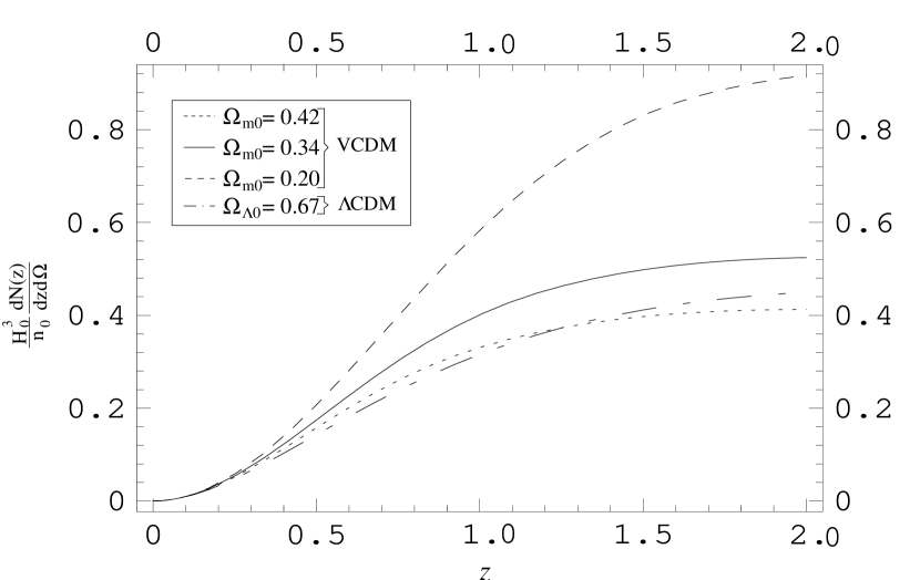
Figure 4: Plot of the predicted number counts of objects per redshift interval and per solid angle, $dN(z)/dzd\Omega$ (normalized by the present number of such objects in the volume $H_{0}^{-3}$) as functions of their redshift $z$, for the spatially flat VCDM (with $\Omega_{m0}=0.34^{+0.08}_{-0.14}$) and $\Lambda$CDM (with $\Omega_{\Lambda 0}=0.67$) models. In this plot, the comoving density is assumed to be constant.

In order to illustrate number counts predicted by the VCDM cosmological model, in figure 4 we plot $dN(z)/dzd\Omega$ given by equation (51), with $H(z)$ given by equation (47). Then, we apply the resulting formula to the spatially flat case and use the parameters obtained in section 5 adopting the HST-Key-Project constraint (see fig. 2), namely $\Omega_{m0}=0.34^{+0.08}_{-0.14}$. Also, we follow Podariu & Ratra (2001) and Loh & Spillar (1986) in assuming, for simplicity, the constancy of the comoving density, $n_{c}(z)=n_{0}a_{0}^{3}$ ($n_{0}$ is the proper density at the present epoch). For sake of comparison, we also plot the spatially flat $\Lambda$CDM prediction, with $\Omega_{\Lambda 0}=0.67$ and the same assumption of constant density. Obviously, the predictions could be improved by dropping this latter assumption and taking into account the density evolution of the observed objects, as mentioned earlier. However, calculating such evolution is beyond the scope of the present paper, not to mention the fact that it is still not completely clear which class of objects we should choose. Moreover, once a more precise $n_{c}(z)$ is known, it is a simple task to take it into account since $dN(z)/dzd\Omega$ is simply proportional to $n_{c}(z)$. From figure 4 we see that the VCDM model predicts more objects to be observed over redshifts $z\lesssim 2$ than the $\Lambda$CDM model. In fact, in a small redshift interval $\Delta z\ll 1$ around $z\approx 1$ the VCDM model predicts approximately $30\%$ more objects than the $\Lambda$CDM model for approximately the same value of $\Omega_{m0}$ (and the same value of $n_{0}/H_{0}^{3}$). Note that this last conclusion should also hold for the counts of galaxies at fixed circular velocities suggested by Newman & Davis (2000), since their comoving density, even though not constant, is very insensitive to the underlying cosmological model at $z\approx 1$. We did not mention here the presence of selection effects, since they highly depend on the measurement procedure itself. Notwithstanding, these effects may also be included in the computation via an “effective” $n_{c}(z)$, which then should be viewed as the number of objects at the spatial section with redshift $z$, per comoving volume, satisfying the detectability conditions.

Measurements of $dN/dzd\Omega$ will provide a valuable way to test the VCDM cosmological model and distinguish it from the $\Lambda$CDM model, when combined with CMBR anisotropy results. Such measurements will soon become available, as the DEEP (Deep Extragalactic Evolutionary Probe) Redshift Survey expects to complete its measurements of the spectra of approximately $65,000$ galaxies in the redshift range $0.7\lesssim z\lesssim 1.5$ by the year 2004.

8 Vacuum Equation of State

The dark-energy equation of state $\rho_{v}=\rho_{v}(p_{v})$ in the VCDM cosmological model with $k=\pm 1$ or $0$ can be easely obtained, for $t>t_{j}$, from equations (29) and (30):

$$\rho_{v}=3p_{v}+\frac{{\bar{m}}^{2}}{8\pi G}\left[1-\left(1+\frac{32\pi G}{{\bar{m}}^{2}}p_{v}\right)^{3/4}\right]\;.$$ (52)

Moreover, from the same pair of equations we also obtain the ratio $w\equiv p_{v}/\rho_{v}$ as a function of redshift:

$$w(z) = \frac{\zeta^{4}-1}{3\zeta^{4}-4\zeta^{3}+1}$$ (53)

$$= \frac{\zeta^{3}+\zeta^{2}+\zeta+1}{3\zeta^{3}-\zeta^{2}-\zeta-1}\;,\;\;0<\zeta<1\;,$$

where $\zeta\equiv a_{j}/a=(1+z)/(1+z_{j})$. Note that equations (29), (30), (52), and (53) are the same as the respective ones presented by Parker & Raval (2001) in dealing with the spatially flat VCDM model. (Note, however, that the spatial curvature changes the value of $z_{j}$; see eqs. [22] and [16].)

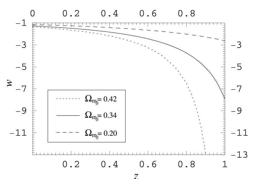
Figure 5: Plot of the predicted ratio $w\equiv p_{v}/\rho_{v}$ as a function of redshift $z$, for the spatially flat VCDM model with $\Omega_{m0}=0.34^{+0.08}_{-0.14}$ (the HST-Key-Project constraint was adopted). The present value of such ratio is $w_{0}=-1.28^{-0.08}_{+0.12}$. Moreover, $w\to-\infty$ as $z\to z_{j-}=(1.19^{-0.19}_{+0.47})_{-}$

In figure 5 we plot the redshift dependence of the ratio $w$, given by equation (53), for the spatially flat VCDM model using the cosmological parameters obtained in section 5 adopting the HST-Key-Project constraint. The present value of this ratio, $w_{0}\equiv w(z=0)$, using $\Omega_{m0}=0.34^{+(0.46;0.08)}_{-0.14}$, is $w_{0}=-1.28^{-(0.91;0.08)}_{+0.12}$. Note, from the expression for $w(z)$, that $w\to-\infty$ as $z\to z_{j-}$, which is simply a consequence of the previously mentioned fact that the vacuum energy approaches a negligibly small value (more rapidly than the vacuum pressure) as $z\to z_{j-}$. That no drastic consequence follows from the divergence of $w$ is evident from figure 6, where we plot, using equations (33) and (36), the ratio $w_{\rm tot}\equiv p/\rho$ between the total pressure $p$ and the total energy density $\rho$ present in the Universe, as a function of redshift. For the sake of comparison, we also plot in the same figure the correspondent ratio $w^{(\Lambda)}_{\rm tot}$ given by the spatially flat $\Lambda$CDM model,

$$w^{(\Lambda)}_{\rm tot} = \frac{p_{r}+p_{\Lambda}}{\rho_{r}+\rho_{m}+\rho_{\Lambda}}$$ (54)

$$= \frac{(\Omega_{r0}/3)(1+z)^{4}-\Omega_{\Lambda 0}}{\Omega_{r0}(1+z)^{4}+(1-\Omega_{r0}-\Omega_{\Lambda 0})(1+z)^{3}+\Omega_{\Lambda 0}}\;,$$

with $\Omega_{\Lambda 0}=0.67$ and $\Omega_{r0}=8.33\times 10^{-5}$. In the VCDM model note that for times earlier than $t_{j}$ (i.e., $z>z_{j}$), during the matter dominated era, the total energy density, $\rho\approx\rho_{m}$, and the total pressure, $p=\rho_{r}/3$, lead to a negligible value of the ratio $w_{\rm tot}$. After $t_{j}$ ($z<z_{j}$), the negative pressure of the vacuum grows very rapidly in magnitude, becoming dominant and determining a very sharp transition to the dark-energy dominated era. This is an important distinction between the VCDM (i.e., vacuum metamorphosis) model and the $\Lambda$CDM model, which presents a rather gradual transition (see fig. 6).

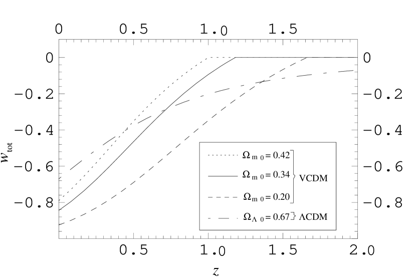
Figure 6: Plot of the ratio $w_{\rm tot}\equiv p/\rho$ as a function of redshift $z$, for the spatially flat VCDM model with $\Omega_{m0}=0.34^{+0.08}_{-0.14}$ and for the spatially flat $\Lambda$CDM model with $\Omega_{\Lambda 0}=0.67$. With these parameters, the present values of $w_{\rm tot}$ and $w^{(\Lambda)}_{\rm tot}$ are $w_{\rm tot}(z=0)=-0.85^{+0.06}_{-0.07}$ and $w^{(\Lambda)}_{\rm tot}(z=0)=-0.67$. Note that for the VCDM model the ratio $w_{\rm tot}$ is negligible for times earlier than $t_{j}$ (i.e., $z>z_{j}$), during the matter dominated era.

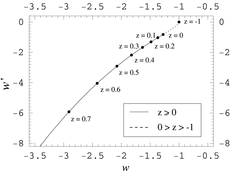
Figure 7: Plot of the curve $\left(w(z),w^{\prime}(z)\right)$, parametrized by the redshift $z$, for the spatially flat VCDM model with $\Omega_{m0}=0.34$. The solid-line curve corresponds to redshift $z\geq 0$ while the dashed-line one corresponds to $-1<z<0$. At the present epoch we have $\left(w_{0},w^{\prime}_{0}\right)=\left(-1.28,-0.8\right)$. Note that $\left(w(z),w^{\prime}(z)\right)\to\left(-1,0\right)$ as $z\to-1$, which means that the dark energy of the VCDM model behaves like a cosmological constant in the asymptotic future.

In order to analyze not only the value of $w$ but also its rate of change in redshift, we plot in figure 7, using $\Omega_{m0}=0.34$, the curve $\left(w(z),w^{\prime}(z)\right)$, where $w^{\prime}(z)\equiv dw(z)/dz$. The redshift $z$ is used as the parameter of the curve. The present value $w^{\prime}_{0}\equiv w^{\prime}(z=0)$ predicted by the spatially flat VCDM model is $w^{\prime}_{0}=-0.8^{-(4.2;0.3)}_{+0.4}$. Note that $w\to-1$ and $w^{\prime}\to 0$ as $z\to-1$, which means that in the asymptotic future (assuming that nothing new will prevent the unbounded expansion of the Universe) the dark energy of the VCDM model behaves like an effective cosmological constant, with value given by $\Lambda_{\rm eff}\equiv{\bar{m}}^{2}/4=5.1^{-(3.2;0.4)}_{+2.1}\times 10^{-66}~{}{\rm eV}^{2}$. For comparison, in a $\Lambda$CDM model with $H_{0}\approx 65$ ${\rm km}~{}{\rm s}^{-1}~{}{\rm Mpc}^{-1}$ and $\Omega_{\Lambda 0}\approx 0.67$, one would have $\Lambda=3\Omega_{\Lambda 0}H_{0}^{2}\approx 3.8\times 10^{-66}~{}{\rm eV}^{2}$.

The experimental determination of $w(z)$, avoiding model-dependent assumptions, relies basically on measurements that, at least in principle, will determine $H(z)$ with sufficient precision to provide also a reliable determination of $H^{\prime}(z)\equiv dH(z)/dz$ (Huterer & Turner, 2001). To see this, let us consider the conservation equation satisfied by the total energy density $\rho$ and the total pressure $p$, namely $d(\rho a^{3})+p\;d\left(a^{3}\right)=0$. Thus, with the (only) assumption that matter and radiation are separately conserved, we have that the energy density, $\rho_{X}$, and pressure, $p_{X}$, of dark energy (whatever it is) also satisfy the same conservation equation, which implies

$$\frac{1}{\rho_{X}}\frac{d\rho_{X}}{dz}=-\frac{(1+w_{X})}{a^{3}}\frac{d\left(a^{3}\right)}{dz}=3\frac{(1+w_{X})}{(1+z)}\;,$$ (55)

where $w_{X}\equiv p_{X}/\rho_{X}$ and we have used $1+z=a_{0}/a$. Considering the general expression for the Hubble parameter as a function of redshift (which is obtained from Einstein’s equation together with the assumption of separate conservation of matter and radiation),

$$\frac{H(z)^{2}}{H_{0}^{2}}=\Omega_{r0}(1+z)^{4}+\Omega_{m0}(1+z)^{3}+\Omega_{k0}(1+z)^{2}+\Omega_{X0}\frac{\rho_{X}(z)}{\rho_{X0}}\;$$ (56)

[with $\rho_{X0}$ being the present value of the dark-energy density and $\Omega_{X0}\equiv 8\pi G\rho_{X0}/(3H_{0}^{2})$], and using it and its redshift derivative to evaluate the left-hand-side of equation (55), we finally obtain the desired expression for $w_{X}(z)$:

$$w_{X}(z) = \frac{(1+z)}{3}\frac{\left[d\rho_{X}(z)/dz\right]}{\rho_{X}(z)}-1$$ (57)

$$= \frac{1}{3}\frac{\left[2(1+z)E^{\prime}(z)-3E(z)\right]E(z)-(1+z)^{2}\left[\Omega_{r0}(1+z)^{2}-\Omega_{k0}\right]}{E(z)^{2}-\Omega_{r0}(1+z)^{4}-\Omega_{m0}(1+z)^{3}-\Omega_{k0}(1+z)^{2}}\;,$$

where, again, $E(z)\equiv H(z)/H_{0}$ and $E^{\prime}(z)\equiv dE(z)/dz$. Thus, as stated above, $w_{X}(z)$ can be found from the determination of $H(z)$ and $H^{\prime}(z)$. The quantity $H(z)$ can be determined from the direct observables $d_{L}(z)$ and $dN(z)/dzd\Omega$, and the quantity $n_{c}(z)$ (Huterer & Turner, 2001). This is done by using equation (45) to express the derivative with respect to $r$ in equation (50) in terms of a derivative with respect to $z$, and then using equation (48) to express $r(z)$ in terms of $d_{L}(z)$. This leads to the following expression for $H(z)$:

$$H(z)=\frac{n_{c}(z)}{a_{0}^{3}}\left(\frac{dN(z)}{dzd\Omega}\right)^{-1}\frac{d_{L}(z)^{2}}{(1+z)^{2}}\;.$$ (58)

Thus, by considering measurements of luminosity distances and number counts, $H(z)$ can be regarded as a directly observable quantity, which gives $w_{X}(z)$ through equation (57). In this sense, future data provided by the proposed satellite SNAP on supernovae luminosity distances (see sec. 6) and by the DEEP redshift survey on number counts (see sec. 7) may greatly improve our knowledge of the dark-energy equation of state.

9 Conclusion

We have shown that the current observational data indicating that the expansion of the Universe is undergoing acceleration are quite consistent with the hypothesis that a transition to a constant-scalar-curvature stage of the expansion occurred at a redshift $z\sim 1$ in the spatially flat FRW universe having zero cosmological constant. This is the scenario proposed in the VCDM (or vacuum metamorphosis) model introduced by Parker and Raval. The late constancy of the scalar curvature at a value $R_{j}=\bar{m}^{2}$ is induced by quantum effects of a free scalar field of low mass in the curved cosmological background. The parameter $\bar{m}$, related to the mass of the field, is the only new relevant parameter introduced in this model, and can be expressed in terms of the present cosmological parameters $H_{0}$, $\Omega_{m0}$, $\Omega_{r0}$, and $\Omega_{k0}$ (see eq. [16]).

Comparison of the CMBR-power-spectrum data with the flat-VCDM-model prediction, without or with the HST-Key-Project result as a constraint (see figs. 1 and 2, and table 1), gives the values of the cosmological parameters to be $H_{0}=65^{-(16;1)}_{+10}$ ${\rm km}$ ${\rm s}^{-1}$ ${\rm Mpc}^{-1}$ and $\Omega_{m0}=0.34^{+(0.46;0.08)}_{-0.14}$. (Recall the definition of our notation in sec. 2: the uncertainties appearing in parenthesis refer to the $95\%$ confidence level, without and with the HST constraint, respectively.) Such values lead to $\bar{m}=4.52^{-(1.76;0.18)}_{+0.84}\times 10^{-33}$ ${\rm eV}$, and the best-fit values from the CMBR data give rise to a very good no-parameter fit to the SNe-Ia observational data. However, the SNe-Ia data are not accurate enough to draw a clear distinction between the VCDM and $\Lambda$CDM models. Other quantities of interest predicted by the VCDM model with the cosmological parameters mentioned above are the time and redshift at the transition between the matter-dominated and constant-scalar-curvature stages, ($t_{j}=5.33^{+(3.41;0.22)}_{-0.84}$ ${\rm Gyr}$ and $z_{j}=1.19^{-(0.76;0.19)}_{+0.47}$), the time and redshift when the accelerated expansion started ($t_{a}=8.0^{+(5.2;0.4)}_{-1.2}$ ${\rm Gyr}$ and $z_{a}=0.67^{-(0.59;0.15)}_{+0.35}$), and the age of the Universe, $t_{0}=14.9\mp 0.8$ ${\rm Gyr}$.

Regarding future tests of the VCDM model, we have presented the prediction of number counts as a function of redshift, and compared it with the analogous $\Lambda$CDM prediction (see fig. 4). For approximately the same cosmological parameters, the VCDM model predicts nearly $30\%$ more objects to be observed in a small redshift interval around $z\approx 1$ than the $\Lambda$CDM model. Data provided by the DEEP Redshift Survey in the near future will likely be able to distinguish these two models. Also, DEEP data combined with future measurements of SNe-Ia luminosity distances provided by the proposed SNAP satellite should greatly improve our knowledge of the dark energy equation of state, which bears the most distinct feature of the VCDM model: $w<-1$ and $w^{\prime}<0$ (see figs. 5 and 7).

It should be noted that we have here considered the simplest form of the VCDM model, in which the transition to constant scalar curvature is continuous and effectively instantaneous (see fig. 6). This form of the model makes definite predictions regarding the distance moduli of SNe-Ia and number counts. Thus, it is encouraging that it remains a viable model when confronted with the current observational data. Other natural parameters that may come into the VCDM model are the time interval over which the transition occurs, and the vacuum expectation value of the scalar field. A nonzero value of the transition time interval would mainly affect the predictions around $z\sim 1$, and a nonzero value of the vacuum expectation value is likely to increase the ratio of pressure to density, $w$. Future observational data will determine if it is necessary to consider nonzero values for these parameters.

References

- Abramo, Tsamis, & Woodard (1999) Abramo, L. R., Tsamis, N. C., & Woodard, R. P. 1999, Fortsch. Phys., 47, 389
- Abroe et al. (2001) Abroe, M. E., et al. 2001, MNRAS, in press (astro-ph/0111010)
- Armendariz-Picon, Mukhanov, & Steinhardt (2001) Armendariz-Picon, C., Mukhanov, V., & Steinhardt, P. J. 2001, Phys. Rev. D, 63, 103510
- Bahcall & Fan (1998) Bahcall, N. A., & Fan, X. 1998, ApJ, 504, 1
- Bassett et al. (2002a) Bassett, B. A., Kunz, M., Silk, J., & Ungarelli, C. 2002a, MNRAS, in press (astro-ph/0203383)
- Bassett et al. (2002b) Bassett, B. A., Kunz, M., Silk, J., & Ungarelli, C. 2002b, preprint (astro-ph/0205428)
- Bean, Hansen, & Melchiorri (2002) Bean, R., Hansen, S. H., & Melchiorri, A. 2002, Nucl. Phys. Proc. Suppl., 110, 167
- Blanchard & Bartlett (1998) Blanchard, A., & Bartlett, J. G. 1998, A&A, 332, L49
- Bond, Jaffe, & Knox (2000) Bond, J. R., Jaffe, A. H., & Knox, L. E. 2000, ApJ, 533, 19
- Caldwell, Dave, & Steinhardt (1998) Caldwell, R., Dave, R., & Steinhardt, P. J. 1998, Phys. Rev. Lett., 80, 1582
- Caldwell (2002) Caldwell, R. 2002, Phys. Lett. B, 545, 23
- Colberg et al. (2000) Colberg, J. M., et al. 2000, MNRAS, 319, 209
- DeWitt (1965) DeWitt, B. S. 1965, Dynamical Theory of Groups and Fields (New York: Gordon and Breach)
- Dodelson, Gates, & Turner (1996) Dodelson, S., Gates, E., & Turner, M. S. 1996, Science, 274, 69
- Dodelson, Kaplinghat, & Stewart (2000) Dodelson, S., Kaplinghat, M., & Stewart, E. 2000, Phys. Rev. Lett., 85, 5276
- Dolgov (1983) Dolgov, A. D. 1983, in The Very Early Universe, ed. G. W. Gibbons, S. W. Hawking, and S. T. C. Siklos (Cambridge: Cambridge University Press)
- Durrer, Novosyadlyj, & Apunevych (2001) Durrer, R., Novosyadlyj, B., & Apunevych, S. 2001, ApJ, submitted (astro-ph/0111594)
- Ford (1987) Ford, L. H. 1987, Phys. Rev. D, 35, 2339
- Ford (2002) Ford, L. H. 2002, preprint (gr-qc/0210096)
- Freedman et al. (2001) Freedman, W. L., et al. 2001, ApJ, 553, 47
- Haiman, Mohr, & Holder (2001) Haiman, Z., Mohr, J. J., & Holder, G. P. 2001, ApJ, 553, 545
- Hu et al. (2001) Hu, W., Fukugita, M., Zaldarriaga, M., & Tegmark, M. 2001, ApJ, 549, 669
- Huterer & Turner (2001) Huterer, D., & Turner, M. S. 2001, Phys. Rev. D, 64, 123527
- Jack & Parker (1985) Jack, I., & Parker, L. 1985, Phys. Rev. D, 31, 2439
- Jackiw (1974) Jackiw, R. 1974, Phys. Rev. D, 9, 1686
- Knox, Christensen, & Skordis (2001) Knox, L., Christensen, N., & Skordis, C. 2001, ApJ, 563, L95
- Krauss (2000) Krauss, L. M. 2000, Phys. Rep., 333, 33
- Krauss & Turner (1995) Krauss, L. M., & Turner, M. S. 1995, Gen. Rel. Grav., 27, 1137
- Loh & Spillar (1986) Loh, E. D., & Spillar, E. J. 1986, ApJ, 307, L1
- Masi et al. (2002) Masi, S., et al. 2002, preprint (astro-ph/0201137)
- Melchiorri et al. (2002) Melchiorri, A., Mersini, L., Odman, C. J., Trodden, M. 2002, preprint (astro-ph/0211522)
- Netterfield et al. (2002) Netterfield, C. B., et al. 2002, ApJ, 571, 604
- Newman & Davis (2000) Newman, J. A., & Davis, M. 2000, ApJ, 534, L11
- Newman et al. (2002) Newman, J. A., Marinoni, C., Coil, A. L., & Davis, M. 2002, PASP, 114, 29
- Ostriker & Steinhardt (1995) Ostriker, J. P., & Steinhardt, P. J. 1995, Nature, 377, 600
- Parker & Toms (1985a) Parker, L., & Toms, D. J. 1985a, Phys. Rev. D, 31, 953
- Parker & Toms (1985b) Parker, L., & Toms, D. J. 1985b, Phys. Rev. D, 31, 2424
- Parker & Toms (1985c) Parker, L., & Toms, D. J. 1985c, Phys. Rev. D, 32, 1409
- Parker & Raval (1999a) Parker, L., & Raval, A. 1999a, Phys. Rev. D, 60, 063512
- Parker & Raval (1999b) Parker, L., & Raval, A. 1999b, Phys. Rev. D, 60, 123502
- Parker & Raval (1999c) Parker, L., & Raval, A. 1999c, preprint (gr-qc/9908069)
- Parker & Raval (2000) Parker, L., & Raval, A. 2000, Phys. Rev. D, 62, 083503
- Parker & Raval (2001) Parker, L., & Raval, A. 2001, Phys. Rev. Lett., 86, 749
- Peebles (1993) Peebles, P. J. E. 1993, Principles of Physical Cosmology (Princeton: Princeton University Press)
- Perlmutter et al. (1998) Perlmutter, S., et al. 1998, Nature, 391, 51
- Perlmutter et al. (1999) Perlmutter, S., et al. 1999, ApJ, 517, 565
- Podariu & Ratra (2001) Podariu, S., & Ratra, B. 2001, ApJ, 563, 28
- Pryke et al. (2002) Pryke, C., Halverson, N. W., Leitch, E. M., Kovac, J., Carlstrom, J. E., Holzapfel, W. L., & Dragovan, M. 2002, ApJ, 568, 46
- Riess et al. (1998) Riess, A. G., et al. 1998, AJ, 116, 1009
- Riess et al. (2001) Riess, A. G., et al. 2001, ApJ, 560, 49
- Schwinger (1951) Schwinger, J. 1951, Phys. Rev., 82, 664
- Seljak & Zaldarriaga (1996) Seljak, U., & Zaldarriaga, M. 1996, ApJ, 469, 437
- Tsamis & Woodard (1998a) Tsamis, N. C., & Woodard, R. P. 1998a, Phys. Lett. B, 426, 21
- Tsamis & Woodard (1998b) Tsamis, N. C., & Woodard, R. P. 1998b, Phys. Rev. D, 57, 4826
- Turner (2001) Turner, M. S. 2001, ApJ, submitted (astro-ph/0106035)
- Viana & Liddle (1999) Viana, P. T. P., & Liddle, A. R. 1999, MNRAS, 303, 535
- Wang, Tegmark, & Zaldarriaga (2002) Wang, X., Tegmark, M., & Zaldarriaga, M. 2002, Phys. Rev. D, 65, 123001
- Zaldarriaga & Seljak (2000) Zaldarriaga, M., & Seljak, U. 2000, ApJS, 129, 431
- Zlatev, Wang, & Steinhardt (1999) Zlatev, I., Wang, L., & Steinhardt, P. J. 1999, Phys. Rev. Lett., 82, 896