Detection of molecular hydrogen in a near Solar-metallicity damped Lyman-$\alpha$ system at $z_{\rm abs}\approx 2$ toward Q 0551$-$366

We report the detection of H₂, C i, C i ^⋆, C i ^⋆⋆ and Cl i lines in a near Solar-metallicity ([Zn/H$]=-0.13$) damped Lyman-$\alpha$ (DLA) system at $z_{\rm abs}=1.962$ observed on the line of sight to the quasar Q 0551$-$366. The iron-peak elements, ${\rm X}={\rm Fe}$, Cr and Mn are depleted compared to zinc, [X/Zn$]\sim-0.8$, probably because they are tied up onto dust grains. Among the three detected H₂-bearing clouds, spanning 55 km s^-1 in velocity space, we derive a total molecular hydrogen column density $N($H${}_{2})=2.6\times 10^{17}$ cm^-2 and a mean molecular fraction $f=2N($H${}_{2})/(2N($H${}_{2})+N($H i$))=1.7\times 10^{-3}$. The depletion of heavy elements (S, Si, Mg, Mn, Cr, Fe, Ni and Ti) in the central component is similar to that observed in the diffuse neutral gas of the Galactic halo. This depletion is approximately the same in the six C i-detected components independently of the presence or absence of H₂. The gas clouds in which H₂ is detected always have large densities, $n_{\rm H}>30$ cm^-3, and low temperatures, $T_{\rm 01}\la 100$ K. This shows that presence of dust, high particle density and/or low temperature are required for molecules to be present. The photo-dissociation rate derived in the components where H₂ is detected suggests the existence of a local UV radiation field similar in strength to the one in the Galaxy. Star formation therefore probably occurs near these H₂-bearing clouds.

1 Introduction

Damped Lyman-$\alpha$ (DLA) absorption line systems observed in the spectrum of quasars are associated with large H i column densities ($N$(H i$)>2\times 10^{20}$ cm^-2). Therefore, they are probably associated with regions of the Universe where star formation occurs (Pettini et al. 1997). It is still unclear whether the gas producing the absorption lines is located in large, fast-rotating protogalactic discs (Wolfe et al. 1986, Prochaska & Wolfe 1997), in interacting building blobs (Haehnelt et al. 1998) or in density fluctuations of galaxy haloes (Ledoux et al. 1998).

Whatever the exact nature of DLA systems may be, molecules (especially H₂) are expected to be found in those clouds. However, despite intensive searches (e.g. Black et al. 1987, Ge & Bechtold 1999, Petitjean et al. 2000) only four detections of H₂ have been reported to date. Recently, a fifth case has been discovered serendipitously by Levshakov et al. (2002) at $z_{\rm abs}=3.025$ toward Q 0347$-$383.

The most recent survey for molecular hydrogen in 11 $z_{\rm abs}>1.8$ DLA systems, capitalizing on the unique capabilities of the UVES high-resolution spectrograph of the ESO Very Large Telescope, has given stringent upper limits, in the range $1.2\times 10^{-7}$ – $1.6\times 10^{-5}$, for the molecular fraction $f=2N($H${}_{2})/(2N($H${}_{2})+N($H i$))$ in nine of the systems (Petitjean et al. 2000). Two possible detections have also been reported at $z_{\rm abs}=2.374$ toward Q 0841$+$129 (Petitjean et al. 2000) and at $z_{\rm abs}=3.390$ toward Q 0000$-$263 (Levshakov et al. 2000) based, however, on the detection of only two weak features located into the Lyman-$\alpha$ forest. Petitjean et al. (2000) concluded that the non-detection of molecular hydrogen in most of the DLA systems could be a direct consequence of high kinetic temperatures, $T>3000$ K, implying low formation rates of H₂ onto dust grains. Therefore, most of the DLA systems probably arise in warm and diffuse neutral gas. Fig. 5 of Petitjean et al. (2000) also suggests that, even if the gas is warm, H₂ should invariably be detected with $f\la 10^{-6}$. Such very low molecular fractions probably result from high ambient UV flux.

In this paper, we present new results obtained from VLT-UVES high resolution spectroscopy of a DLA system at $z_{\rm abs}=1.962$ toward Q 0551$-$366. Details of the observations are given in Sect. 2. The metal content, dust depletion pattern and H₂ molecular content of the absorber are discussed in, respectively, Sects. 3, 4 and 5. Our results are finally summarized and their implications discussed in Sect. 6.

2 Observations

The Ultraviolet and Visible Echelle Spectrograph (UVES; see Dekker et al. 2000) mounted on the ESO Kueyen VLT-UT2 8.2 m telescope on Cerro Paranal in Chile has been used in the course of a survey to search for H₂ absorption lines in a sample of DLA systems.

High-resolution, high signal-to-noise ratio spectra of the $m_{\rm V}=17.6$, $z_{\rm em}=2.32$ Q 0551$-$366 quasar were obtained on October 20-23, 2000. Standard settings were used in both blue and red arms with Dichroic #1 (central wavelengths: 3460 and 5800 Å) and central wavelengths were adjusted to 4370 Å in the Blue (7500 Å in the Red) with Dichroic #2. This way, full wavelength coverage was obtained from 3050 to 7412 Å and from 7566 to 9396 Å accounting for the gap between red-arm CCDs. The CCD pixels were binned $2\times 2$ in both arms and the slit width was fixed to $1\arcsec$ yielding a spectral resolution $R=42500$. The total integration times were 5 hours using Dichroic #1 and 2h15min using Dichroic #2.

The data have been reduced with the UVES pipeline (Ballester et al. 2000) which is available as a context of the ESO MIDAS data reduction system. The main characteristics of the pipeline is to perform a precise inter-order background subtraction, especially for master flat-fields, and to allow for an optimal extraction of the object signal rejecting cosmic rays and performing sky-subtraction at the same time. The pipeline products were checked step by step. We then converted the wavelengths of the reduced spectra to vacuum-heliocentric values and scaled, weighted and combined together individual 1D exposures using the NOAO onedspec package of the IRAF software. The resulting unsmoothed spectra were re-binned to the same wavelength step, 0.0471 Å pix^-1, yielding an average signal-to-noise ratio per resolution element as high as 10 at 3200 Å, 25 at 3700 Å and 60 at 6000 Å.

3 Metal content

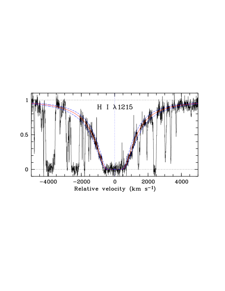
Figure 1: Portion of the normalized VLT-UVES spectrum showing the damped Lyman-$\alpha$ line at $z_{\rm abs}=1.962$ toward Q 0551$-$366. The best Voigt-profile fitting, $N($H i$)=(3.2\pm 0.6)\times 10^{20}$ cm^-2, is superimposed onto the data.

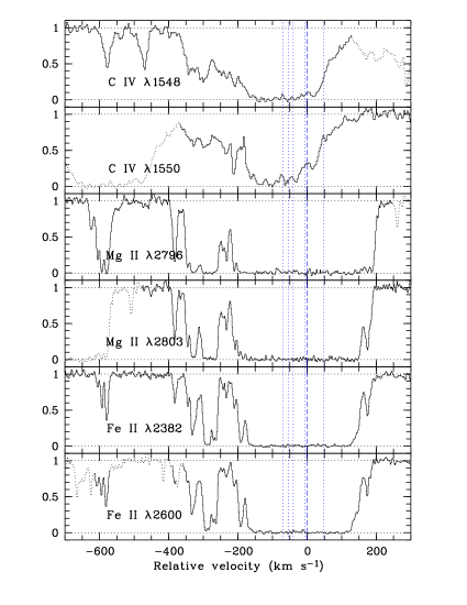
Figure 2: Absorption profiles related to the C iv $\lambda\lambda$1548,1550, Mg ii $\lambda\lambda$2796,2803 and Fe ii $\lambda\lambda$2382,2600 transition lines. Blended parts of the profiles are shown by dotted histogrammes. The location of the C i-detected components (see Fig. 4) is indicated by vertical lines with the origin of the velocity scale corresponding to $z_{\rm abs}=1.96221$.

   

   

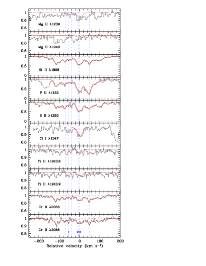
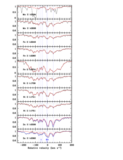
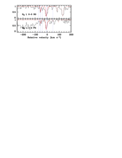
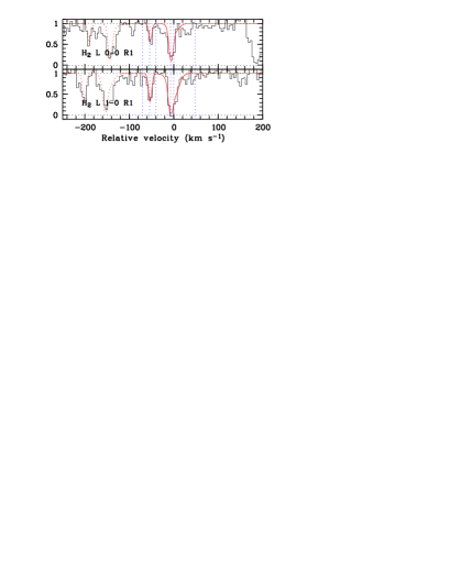
Figure 3: Comparison of the velocity profiles of metal lines (upper panels) with a few of the H₂ lines (lower panels) observed at $z_{\rm abs}=1.962$ toward Q 0551$-$366. The best fitting is superimposed onto the spectra. The position of the six components detected in C i is shown by vertical lines. The three components where H₂ is detected are given numbers.
Upper panels: for the fitting of the Zn ii $\lambda$2026 (resp. Zn ii $\lambda$2062) profile (light curves), the blending with Mg i (resp. Cr ii) lines has been carefully taken into account by fitting Mg i $\lambda\lambda$2026,2852, Cr ii $\lambda\lambda\lambda$2056,2062,2066 and Zn ii $\lambda\lambda$2026,2062 altogether (dark curves). Lower panels: dotted parts of the synthetic profiles correspond to other H₂ transitions than the ones indicated.

Table 1: Atomic data

Transition	$\lambda_{\rm vac}$	$f$	Ref.
	(Å)
H i $\lambda$1215	1215.6701	0.4164	a
C i $\lambda$1560	1560.3092	0.0719	b
C i ${}^{\star}\lambda$1560.6	1560.6822	0.0539	b
C i ${}^{\star}\lambda$1560.7	1560.7090	0.0180	b
C i ${}^{\star\star}\lambda$1561.3	1561.3402	0.0108	b
C i ${}^{\star\star}\lambda$1561.4	1561.4384	0.0603	b
C i $\lambda$1656	1656.9283	0.139	b
C i ${}^{\star}\lambda$1656.2	1656.2672	0.0589	b
C i ${}^{\star}\lambda$1657.3	1657.3792	0.0356	b
C i ${}^{\star}\lambda$1657.9	1657.9068	0.0473	b
C i ${}^{\star\star}\lambda$1657.0	1657.0082	0.104	b
C i ${}^{\star\star}\lambda$1658.1	1658.1212	0.0356	b
Mg ii $\lambda$1239	1239.9253	0.000554	c
Mg ii $\lambda$1240	1240.3947	0.000277	c
Si ii $\lambda$1808	1808.0129	0.00208	d
P ii $\lambda$1152	1152.8180	0.236	a
P ii $\lambda$1532	1532.5330	0.00761	a
S ii $\lambda$1250	1250.5780	0.00545	a
Cl i $\lambda$1188	1188.7742	0.0728	a
Cl i $\lambda$1347	1347.2396	0.153	e
Ti ii $\lambda$1910.6	1910.6090	0.104	f
Ti ii $\lambda$1910.9	1910.9380	0.098	f
Cr ii $\lambda$2056	2056.2569	0.105	g
Cr ii $\lambda$2062	2062.2361	0.0780	g
Cr ii $\lambda$2066	2066.1640	0.0515	g
Mn ii $\lambda$2594	2594.4990	0.271	a
Mn ii $\lambda$2606	2606.4619	0.193	a
Fe ii $\lambda$2249	2249.8768	0.00182	h
Fe ii $\lambda$2260	2260.7805	0.00244	h
Fe ii $\lambda$2374	2374.4603	0.0313	i
Ni ii $\lambda$1709	1709.6042	0.0324	j
Ni ii $\lambda$1741	1741.5531	0.0427	j
Ni ii $\lambda$1751	1751.9157	0.0277	j
Zn ii $\lambda$2026	2026.1371	0.489	g
Zn ii $\lambda$2062	2062.6604	0.256	g

From Voigt-profile fitting to the damped Lyman-$\alpha$ line, we find that the total neutral hydrogen column density of the system at $z_{\rm abs}=1.962$ toward Q 0551$-$366 is $\log N($H i$)=20.50\pm 0.08$ (see Fig. 1). The associated metal line profiles of low-ionization species are complex and span up to 850 km s^-1 in velocity space as observed from the Mg ii $\lambda\lambda$2796,2803 and Fe ii $\lambda\lambda$2382,2600 transitions (Fig. 2). In Fig. 3, we display the strongest part of the profiles, in the range [$-250$,$+200$] km s^-1 relative to $z_{\rm abs}=1.96221$, for a large number of ions. The (optically thin) line profiles were fitted together using the fitlyman programme (Fontana & Ballester 1995) running under MIDAS, and/or vpfit (Carswell et al., http://www.ast.cam.ac.uk/$\sim$rfc/vpfit.html). The oscillator strength values compiled in Table 1 were used.

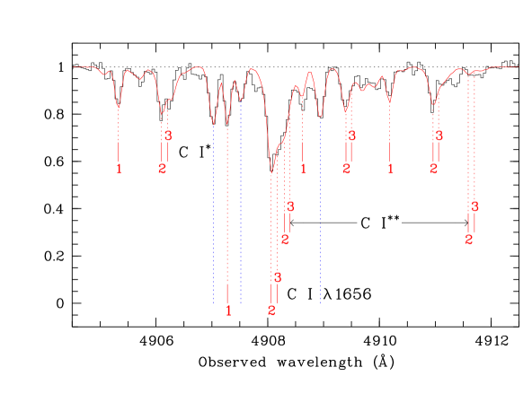
Figure 4: Absorption profile due to C i $\lambda$1656.9, C i ${}^{\star}\lambda\lambda\lambda$1656.2,1657.3,1657.9 and C i ${}^{\star\star}\lambda\lambda$1657.0,1658.1 transition lines at $z_{\rm abs}=1.962$. A total of six C i components is detected over 120 km s^-1. The three components where H₂ and C i ^⋆ absorption lines are both detected are indicated by numbers and vertical bars.

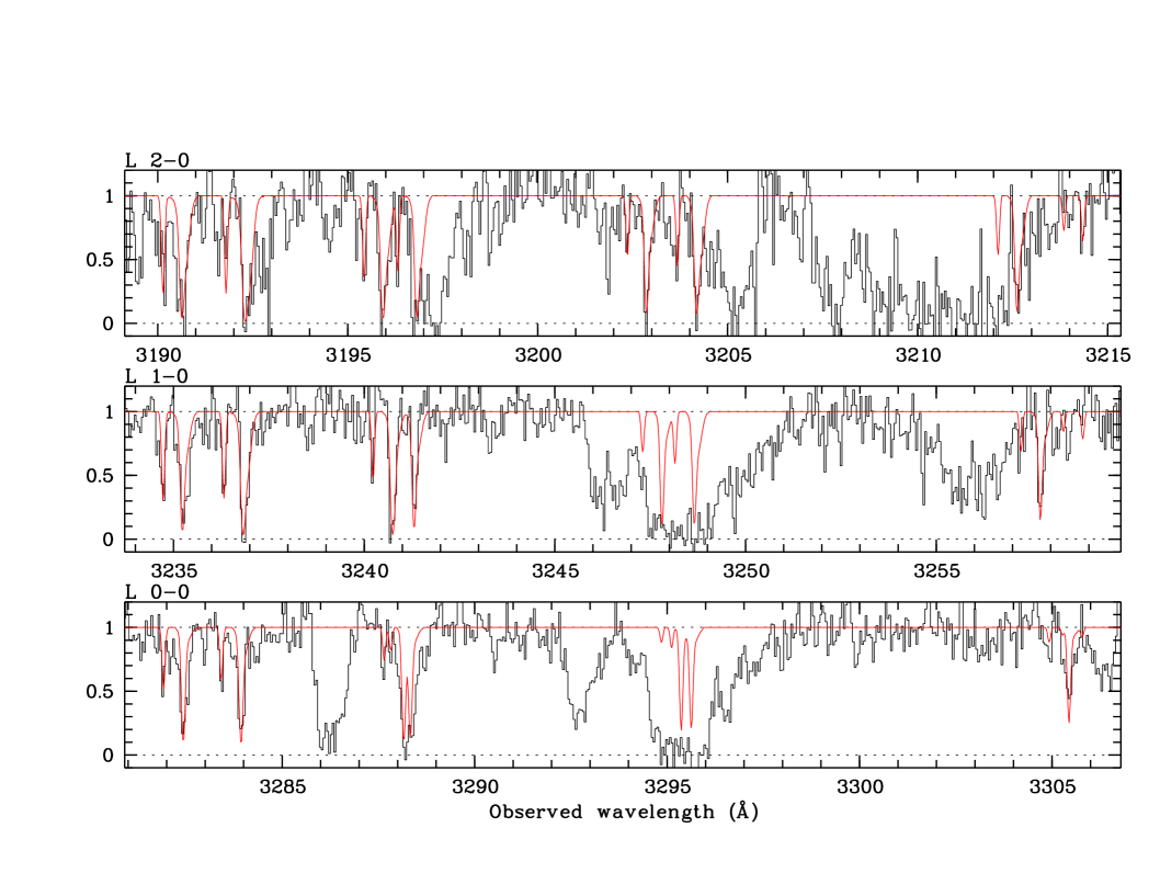
Figure 5: Selected transition lines from the $J=0$, 1, 2, 3 and 4 rotational levels of the vibrational ground-state of H₂ at $z_{\rm abs}=1.962$. H₂ molecules are detected in three different clouds with velocity separations ranging from 7 to 55 km s^-1.

Among the metal components, no less than six are detected in C i whose absorption line profiles are spread over $120$ km s^-1. The C i $\lambda\lambda$1560,1656 complexes have been fitted simultaneously thereby ensuring uniqueness of the fitting solution given that the relative positions of the C i, C i ^⋆ and C i ^⋆⋆ lines are different in the two wavelength ranges. Among the C i components, three actually show absorption lines from C i ^⋆, out of which two also show lines from C i ^⋆⋆ (see Fig. 4). Absorption lines due to different rotational levels of H₂ in its vibrational ground state (see Fig. 5) are detected in three of the components producing detectable C i ^⋆ lines.

Table 2: Metal abundances from the C i-detected components of the DLA system toward Q 0551$-$366

$z_{\rm abs}$	Ion	$\log N$	[X/H$]^{\rm a}$
1.962	H i	$20.50\pm 0.08$	…
	Si ii	$15.62\pm 0.06$	$-0.43\pm 0.10$
	P ii	$<14.03$	$<-0.04$
	S ii	$15.38\pm 0.11$	$-0.39\pm 0.14$
	Cr ii	$13.27\pm 0.06$	$-0.91\pm 0.10$
	Mn ii	$13.11\pm 0.05$	$-0.92\pm 0.09$
	Fe ii	$15.05\pm 0.05$	$-0.96\pm 0.09$
	Ni ii	$14.08\pm 0.06$	$-0.67\pm 0.10$
	Zn ii	$13.02\pm 0.05$	$-0.13\pm 0.09$

Table 3: Column densities of metal ions in C i-detected components

Ion	Transition	$\log N$	$b$
	lines used		(km s-1)
$z_{\rm abs}=1.96150$
Si ii	1808	$14.78\pm 0.03$a	$8.4\pm 0.6$b
P ii	1152,1532	$12.99\pm 0.11$a	”
S ii	1250	$14.60\pm 0.10$a	”
Cr ii	2056,2062,2066	$12.44\pm 0.04$a	”
Mn ii	2594,2606	$12.37\pm 0.04$a	”
Fe ii	2249,2260,2374a	$14.27\pm 0.02$a	”
Ni ii	1709,1741,1751	$13.34\pm 0.03$a	”
Zn ii	2026,2062	$12.11\pm 0.05$a	”
$z_{\rm abs}=1.96167$
Si ii	1808	$14.37\pm 0.05$a	$3.1\pm 0.5$b
P ii	1152,1532	$12.48\pm 0.25$a	”
S ii	1250	$14.01\pm 0.27$a	”
Cr ii	2056,2062,2066	$11.94\pm 0.09$a	”
Mn ii	2594,2606	$11.70\pm 0.11$a	”
Fe ii	2249,2260,2374a	$13.78\pm 0.04$a	”
Ni ii	1709,1741,1751	$12.80\pm 0.06$a	”
Zn ii	2026,2062	$11.67\pm 0.06$a	”
$z_{\rm abs}=1.96180$
Si ii	1808	$14.37\pm 0.08$a	$4.9\pm 0.6$b
P ii	1152,1532	$12.51\pm 0.25$a	”
S ii	1250	$14.23\pm 0.19$a	”
Cr ii	2056,2062,2066	$12.14\pm 0.08$a	”
Mn ii	2594,2606	$11.91\pm 0.06$a	”
Fe ii	2249,2260,2374a	$13.89\pm 0.05$a	”
Ni ii	1709,1741,1751	$12.95\pm 0.06$a	”
Zn ii	2026,2062	$11.92\pm 0.05$a	”
$z_{\rm abs}=1.96203,1.96212,1.96225$b
Mg ii	1239,1240	$\leq 15.42\pm 0.10$a	$21.2\pm 1.1$b
Si ii	1808	$15.34\pm 0.06$a	”
P ii	1152,1532	$<13.73$a	”
S ii	1250	$15.12\pm 0.07$a	”
Cl i	1188,1347	$12.87\pm 0.09$a	”
Ti ii	1910.6,1910.9	$\leq 12.40\pm 0.09$a	”
Cr ii	2056,2062,2066	$12.96\pm 0.06$a	”
Mn ii	2594,2606	$12.80\pm 0.04$a	”
Fe ii	2249,2260,2374a	$14.75\pm 0.05$a	”
Ni ii	1709,1741,1751	$13.79\pm 0.06$a	”
Zn ii	2026,2062	$12.74\pm 0.05$a	”
$z_{\rm abs}=1.96268$
Si ii	1808	$14.94\pm 0.03$a	$8.0\pm 0.6$b
P ii	1152,1532	$<13.58$a	”
S ii	1250	$14.63\pm 0.11$a	”
Cr ii	2056,2062,2066	$12.67\pm 0.03$a	”
Mn ii	2594,2606	$12.46\pm 0.05$a	”
Fe ii	2249,2260,2374a	$14.39\pm 0.03$a	”
Ni ii	1709,1741,1751	$13.35\pm 0.04$a	”
Zn ii	2026,2062	$12.39\pm 0.03$a	”

It is likely that most, if not all, of the neutral hydrogen originates from the C i components. Therefore, we derive total metal abundances using column densities of singly ionized species summed up over the detected C i components (see Table 2). The result of fitting to individual components is presented in Table 3. Weak additional, undetected C i components cannot represent more than 15 per cent of the total C i column density (i.e. 0.06 dex). The best-fitting curves shown in Fig. 3 have been determined in two steps. In order to derive accurate $b$ values, we first fitted transition lines from Fe ii covering a wide range of oscillator strengths with 22 components, six of which are C i-detected. Using fixed $b$ values as previously measured, we then fitted altogether the lines from Si ii, P ii, S ii, Cr ii, Mn ii, Fe ii, Ni ii and Zn ii. For a given component, the same Doppler parameter and redshift were used for all species. Due to the smoothness of the metal line profiles (see Fig. 3), we did not impose the Doppler parameters from the fitting to C i lines. It is well known that noise leads to overestimate the width of weak lines. Small shifts ($<3$ km s^-1) between the positions of the components in the metal and C i line profiles can be noted as well (see Tables 3 and 5). They are smaller than half of the FWHM of the observations however. This implies that the uncertainty on the absolute metallicities is of the order of 30% but this is much smaller on the abundance ratios.

The metallicity of the gas derived from the absolute abundance of zinc is close to Solar, [Zn/H$]=-0.13$. This is the first time such a high metallicity is observed in a DLA system at high redshift. The abundance of S relative to Zn is not oversolar but is on the contrary slightly undersolar, in agreement with the observations of Galactic thin disk stars (see Chen et al. 2002 and refs. therein). The iron-peak elements (${\rm X}={\rm Fe}$, Cr and Mn) are depleted compared to zinc, [X/Zn$]\sim-0.8$, probably because they are tied up onto dust grains. This is consistent with Si being slightly depleted compared to Zn.

4 Dust depletion pattern

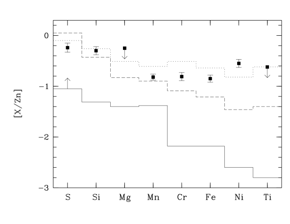
Figure 6: Depletion of heavy elements relative to zinc in the main sub-system (components at $z_{\rm abs}=1.96203$, 1.96212 and 1.96225) of the near Solar-metallicity DLA system toward Q 0551$-$366. The histogrammes show the values observed in cold (continuous line) and warm (dashed line) Galactic disc clouds, and warm Galactic halo clouds (dotted line; from Sembach & Savage 1996).

We compare in Fig. 6 the abundance pattern observed in the main (central) component, where absorption lines from a large number of heavy elements are detected (see Table 3), with the abundance patterns observed in different Galactic environments. To compute the depletion of an element relative to the abundance of zinc, we use the definition [X/Zn$]=\log[N($X$)/N($Zn$)]-\log[N($X$)/N($Zn$)]_{\odot}$ together with the Solar abundances from Savage & Sembach (1996). The error bars on the measurements are $1\sigma$ uncertainties. The continuous and dashed lines are the mean observed trends in the Galactic disc for cold and warm gas respectively, while the dotted line shows the abundance pattern of diffuse gas in the Galactic halo (from Sembach & Savage 1996). It is clear from Fig. 6 that the relative abundance pattern of this near Solar-metallicity DLA system is close to that observed in Galactic warm halo clouds.

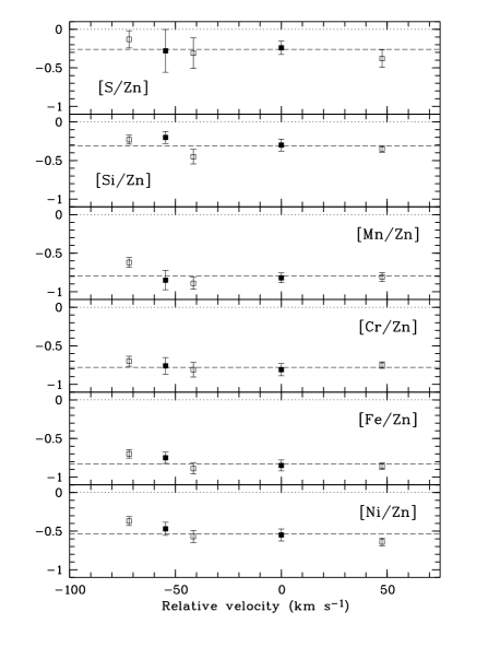
Figure 7: Depletion of heavy elements relative to Zn in the velocity sub-systems where C i is detected. The metal components at $z_{\rm abs}=1.96203$, 1.96212 and 1.96225 (see Table 3) are considered as a single sub-system at $z_{\rm abs}=1.96221$ ($V=0$ km s^-1). The horizontal dashed lines show the column density weighted-mean values of the ratios. Although the depletion pattern is similar in every components, only two of them (shown as filled squares) have detectable H₂ lines: this demonstrates that the presence of H₂ is not only related to the dust-to-metal ratio.

So as to probe any possible velocity dependence of the depletion pattern, we show in Fig. 7 the metal abundance ratios [X/Zn] measured in the C i-detected components. The horizontal dashed lines give the column density weighted-mean values of the abundance ratios. It is apparent that every component, whether absorption lines due to H₂ are present or not, show similar abundance patterns, and as a consequence similar dust-to-metal ratios, within observational uncertainties. This clearly demonstrates that in this DLA system the presence of molecules is not only related to the dust-to-metal ratio. This also suggests in this case that the gas has undergone uniform mixing of heavy elements.

A word of caution should be said here. Whereas the $-55$ km s^-1 component is clearly identified in the metal line profiles, this is not the case of the central components. The overall profiles of most of the metal lines are smooth with no predominant component. However, it is apparent from the Si ii profile that the narrow component at $z_{\rm abs}=1.96214$ ($V=-7$ km s^-1) is present at the bottom of the profile. This means that absorption lines due to the cold gas, i.e. related to C i components, can possibly be hidden by a more pervasive medium. This implies that absolute metallicities are not accurately determined in the neutral gas phase. This is probably not important for volatile elements as the dominant components actually produce the strongest lines, but could be of importance for Fe co-production elements which can be depleted. Consequently, absorption lines from the latter elements can be weak and lost in the overall profiles, which means we may underestimate the depletion factors in the central components and, in particular, the one at $z_{\rm abs}=1.96214$. As an example, a large depletion factor has been derived in a well-defined, weak H₂ component at $z_{\rm abs}=1.968$ observed on the line of sight to Q 0013$-$004 (Petitjean et al. 2002).

Note that Cl i is detected in the main component of the DLA system toward Q 0551$-$366, at $z_{\rm abs}=1.96221$, with $\log N($Cl i$)=12.87\pm 0.09$ (see Table 3). This translates to [Cl/Zn$]=-0.49\pm 0.10$ under the assumption that [Cl i$]\equiv[$Cl]. This is close to what is observed in the Galactic interstellar medium (ISM) toward 23 Ori (Welty et al. 1999). The small value of this ratio is probably a consequence of Cl i being partially ionized. This first detection of neutral chlorine in a DLA system should be related to the high metallicity of the gas as well as to the presence of H₂ with which Cl ii rapidly reacts to form Cl i.

5 H₂ molecular content

Table 4: Voigt-profile fitting results for different rotational levels of the vibrational ground-state transition lines of H₂

$z_{\rm abs}$	Level	$\log N($H${}_{2})$	$b$	$T_{\rm ex}$	Jex
			(km s-1)	(K)
1.96168	$J=0$	$15.19^{+0.46}_{-0.13}$	$2.1\pm 0.7$	…
	$J=1$	$15.23^{+0.33}_{-0.14}$	”	$76\pm 7$	0-1
	$J=2$	$14.76^{+0.27}_{-0.09}$	”	$248\pm 52$	0-2
	$J=3$	$14.72^{+0.18}_{-0.06}$	”	$281\pm 36$	0-3
	$J=4$	$<14.19^{\rm a}$	”	$<680$	0-4
	$J=5$	$<14.34^{\rm a}$	”	$<671$	0-5
1.96214	$J=0$	$16.83^{+0.47}_{-1.09}$	$2.1\pm 0.8$	…
	$J=1$	$17.12^{+0.46}_{-0.69}$	”	$81\pm 29$	0-1
	$J=2$	$16.56^{+0.84}_{-0.80}$	”	$378\pm 255$	0-2
	$J=3$	$16.24^{+1.12}_{-0.59}$	”	$378\pm 243$	0-3
	$J=4$	$14.35^{+0.05}_{-0.13}$	”	$420\pm 178$	0-4
	$J=5$	$<14.34^{\rm a}$	”	$<556$	0-5
1.96221	$J=0$	$14.74^{+0.05}_{-0.13}$	$12.8\pm 1.7$	…
	$J=1$	$15.18^{+0.03}_{-0.05}$	”	$97\pm 40$	0-1
	$J=2$	$14.93^{+0.02}_{-0.16}$	”	$357\pm 69$	0-2
	$J=3$	$14.96^{+0.01}_{-0.11}$	”	$352\pm 43$	0-3

Lyman-band absorption lines from H₂ are detected in two well-detached sub-systems at $z_{\rm abs}=1.96168$ and 1.9622 ($\Delta V\approx 55$ km s^-1) (see Fig. 3 and 5). The former sub-system, corresponding to the C i component labelled “1” in Fig. 3, is narrow and weak but clearly detected in the $J=0$, 1, 2 and 3 rotational levels of the vibrational ground-state of H₂. The latter sub-system, corresponding to C i components “2” and “3”, is broader and stronger. In this case, all unblended lines from the $J=0$, 1, 2 and 3 levels have been fitted together assuming the presence of two components at $z_{\rm abs}=1.96214$ and 1.96221 as observed in C i. The column density for each $J$ level was determined from several trials of Voigt-profile fitting using the oscillator strength values from Morton & Dinerstein (1976). The results are given in Table 4. Errors in the column densities were estimated taking into account the range of possible $b$ values (from the fitting to C i lines) and the level of saturation introduced by background subtraction uncertainties ($\sim 5$%). Errors in the column densities therefore correspond to a range of column densities and not to the rms error from fitting the Voigt profiles. The fifth Column of Table 4 gives the measured excitation temperatures relative to the $J=0$ level (see Srianand & Petitjean 1998). The mean and the error in the excitation temperatures were obtained from all the individual Voigt-profile fittings previously discussed.

The $z_{\rm abs}=1.96214$ component alone corresponds to 95 per cent of the total H₂ column density of the absorber, $N($H${}_{2})=2.6\times 10^{17}$ cm^-2. Note that, even if $b<1$ km s^-1 in the $z_{\rm abs}=1.96214$ component, the total H₂ column density can not exceed $10^{18}$ cm^-2. Unfortunately, the molecular fractions in individual components cannot be determined as the respective H i column densities are not known. The mean molecular fraction along the line of sight is $f=1.7\times 10^{-3}$. The kinetic temperature in H₂-bearing clouds can be approximated to a first order by the excitation temperature $T_{01}$ measured between the $J=0$ and 1 levels. We find $T_{01}=76\pm 7$, $81\pm 29$ and $97\pm 40$ K at $z_{\rm abs}=1.96168$, 1.96214 and 1.96221 respectively. These values are typical of what is measured in the halo of our Galaxy and along lines of sight through the LMC and SMC (Shull et al. 2000, Tumlinson et al. 2002) and are similar to what is derived in different components at $z_{\rm abs}=2.34$ toward Q 1232$+$082 and $z_{\rm abs}=1.97$ toward Q 0013$-$004 (Srianand et al. 2000, Petitjean et al. 2002).

Excitation temperatures for higher $J$ levels are also given in Table 4. In the case of the components at, respectively, $z_{\rm abs}=1.96168$ and 1.96221 toward Q 0551$-$366, the high $J$ level populations can be explained by a single excitation temperature within measurement uncertainties (respectively $T_{\rm ex}\approx 270$ and 350 K). These values are larger than the measured kinetic temperatures. This suggests that, in addition to collisions, other processes like UV pumping and formation pumping are at play to populate these levels. In the case of the $z_{\rm abs}=1.96214$ component, line blending, uncertainty in the position of the zero level and possible saturation of the low $J$ lines actually result in large errors in the column density measurement, and a single excitation temperature, $T_{\rm ex}\approx 380$ K, is also consistent with the observed high $J$ level populations. Incidentally, similar population ratios are observed along lines of sight through the Magellanic stream (Sembach et al. 2001, Richter et al. 2001).

6 Discussion

Table 5: Physical conditions in individual components

$z_{\rm abs}$	$\log N($C i$)$	$\log N($C i ${}^{\star})$	$\log N($C i ${}^{\star\star})$	$b$	$T_{\rm CMB}$	$T_{\rm 01}$	$n_{\rm H}$
				(km s-1)	(K)	(K)	(cm-3)
1.96152	$12.69\pm 0.07$	$<12.18$ :	$<11.94$ :	0$4.3\pm 1.4$	$\leq 10.5$	…	$<17$
1.96168	$12.64\pm 0.07$	$12.84\pm 0.07$	$<12.16$ :	0$2.1\pm 0.7$	$\leq 22.3$	$76\pm\phantom{0}7$	$170-185$
1.96180	$12.42\pm 0.13$	$<12.18$ :	$<11.94$ :	0$3.9\pm 2.3$	$\leq 12.9$	…	$<56$
1.96214	$12.66\pm 0.12$	$12.69\pm 0.11$	$12.11\pm 0.34$	0$2.1\pm 0.8$	$\leq 18.7$	$81\pm 29$	$\phantom{0}55-390$
1.96221	$13.16\pm 0.06$	$12.98\pm 0.09$	$12.26\pm 0.36$	$12.8\pm 1.7$	$\leq 14.5$	$97\pm 40$	$\phantom{0}30-150$
1.96268	$12.63\pm 0.08$	$<12.18$ :	$<11.94$ :	0$4.0\pm 1.8$	$\leq 10.0$	…	$<25$

Considering the cosmic microwave background radiation (CMBR) to be the only source of C i excitation (e.g. Srianand et al. 2000), we can derive upper limits on the CMBR temperature from the column densities of C i, C i ^⋆ and C i ^⋆⋆ that we measure in different components of the DLA system toward Q 0551$-$366 (see Table 5). In the components where H₂ is detected, the values are found to be much larger than what is predicted from standard Big-Bang cosmology (i.e. about 8 K). Under the conditions prevailing in these clouds, fluorescence is negligible in populating the excited levels of C i (see Fig. 2 of Silva & Viegas 2002). This means that excitation by collisions is important and, therefore, that the influence of local physical conditions (both density and temperature) is substantial in those clouds. Conversely, assuming the CMBR temperature to be 8 K and the kinetic temperature being approximated by the excitation temperature of the $J=1$ rotational level, we can estimate the hydrogen density from the relative populations of the C i fine-structure levels. For the components where H₂ is not detected, we assume $T_{\rm kin}=100$ K. As can be seen from Table 5, it is apparent that the densities are larger in the gas where H₂ is detected. Therefore, the non-detection of H₂ in components having similar dust-to-metal ratios and similar column densities of heavy elements is a consequence of lower densities and possibly higher temperatures. This is in line with the conclusions of Petitjean et al. (2000). The allowed range in pressure $p/k$ measured in the three H₂ components are respectively 12950$-$13770, 6050$-$20280 and 4170$-$8550 cm^-3 K. Such high pressures are seen only in $\leq 3$% of the C i gas of our Galaxy (Jenkins & Tripp 2001) but are consistent with the high pressures also derived in the case of Q 0013$-$004 (Petitjean et al. 2002). They probably indicate that the gas under consideration is undergoing high compression due to either collapse, merging and/or supernovae explosions.

It is difficult to measure the rate of H₂ formation onto dust grains in DLA systems because it is related to the amount of dust which is itself difficult to estimate. In the present DLA system, even if the mean metallicity is close to solar the observed mean depletion of Fe is an order of magnitude smaller than what is typically measured in Galactic cold disc clouds. Therefore, we can estimate that the rate of H₂ formation onto dust grains is about one tenth of the Galactic value, thus $R\sim 3\times 10^{-18}$ cm³ s^-1. Using the simple model proposed by Jura (1975) and the column densities and densities estimated above, we derive the photo-absorption rate of the Lyman and Werner bands of H₂: $\beta_{0}=1.4\times 10^{-11}-2.8\times 10^{-10}$ s^-1 for the component at $z_{\rm abs}=1.96214$. This value is similar to the average value measured in the Galactic ISM, $\beta_{0}=5\times 10^{-10}$ s^-1, while the average for the intergalactic radiation field is $\beta_{0}\approx 2\times 10^{-12}$ s^-1 with $J_{21}({\rm 912\leavevmode\nobreak\ \AA})=1$. This shows that there is in-situ star-formation close to the absorbing clouds and that H₂ can survive, at least with such molecular fractions, even in the presence of a strong UV radiation field because the gas has a high particle density. One should keep in mind that the rate of H₂ formation goes linearly with the density of dust grains while it goes as the second power of the H i density. Therefore, it is natural that, even though the presence of dust is a crucial factor for the formation of molecules, local physical conditions such as particle density, temperature and local UV field, play an important role in governing the molecular fraction of a given cloud in DLA systems.

- (1) Ballester, P., Modigliani, A., Boitquin, O., et al. 2000, The Messenger, 101, 31
- (2) Bergeson, S. D., & Lawler, J. E. 1993a, ApJ, 408, 382
- (3) Bergeson, S. D., & Lawler, J. E. 1993b, ApJ, 414, L137
- (4) Bergeson, S. D., Mullman, K. L., & Lawler, J. E. 1994, ApJ, 435, L157
- (5) Bergeson, S. D., Mullman, K. L., Wickliffe, W. E., et al. 1996, ApJ, 464, 1044
- (6) Biémont, E., Gebarowski, R., & Zeippen, C. J. 1994, A&A, 287, 290
- (7) Black, J. H., Chaffee, F. H. Jr., & Foltz C. B. 1987, ApJ, 317, 442
- (8) Chen, Y. Q., Nissen, P. E., Zhao, G., & Asplund, M. 2002, A&A, in press, astro-ph/0206075
- (9) Dekker, H., D’Odorico, S., Kaufer, A., Delabre, B., & Kotzlowski, H. 2000, Proc. SPIE, Vol. 4008, p. 534
- (10) Fedchak, J. A., Wiese, L. M., & Lawler, J. E. 2000, ApJ, 538, 773
- (11) Fontana, A., & Ballester, P. 1995, The Messenger, 80, 37
- (12) Ge, J., & Bechtold, J. 1999, in Carilli C. L., Radford S. J. E., Menten K. M., & Langston G. I., eds., Highly redshifted Radio Lines, ASP Conf. Series, Vol. 156, p. 121
- (13) Haehnelt, M. G., Steinmetz, M., & Rauch, M. 1998, ApJ, 495, 647
- (14) Jenkins, E. B., & Tripp, T. M. 2001, ApJS, 137, 297
- (15) Jura, M. 1975, ApJ, 197, 581
- (16) Ledoux, C., Petitjean, P., Bergeron, J., Wampler, E. J., & Srianand, R. 1998, A&A, 337, 51
- (17) Levshakov, S. A., Molaro, P., Centurión, M., et al. 2000, A&A, 361, 803
- (18) Levshakov, S. A., Dessauges-Zavadsky, M., D’Odorico, S., & Molaro, P. 2002, ApJ, 565, 696
- (19) Morton, D. C. 1991, ApJS, 77, 119
- (20) Morton, D. C., & Dinerstein, H. L. 1976, ApJ, 204, 1
- (21) Petitjean, P., Srianand, R., & Ledoux, C. 2000, A&A, 364, L26
- (22) Petitjean, P., Srianand, R., & Ledoux, C. 2002, MNRAS, 332, 383
- (23) Pettini, M., Smith, L. J., King, D. L., & Hunstead, R. W. 1997, ApJ, 486, 665
- (24) Prochaska, J. X., & Wolfe, A. M. 1997, ApJ, 474, 140
- (25) Richter, P., Sembach, K. R., Wakker, B. P., & Savage, B. D. 2001, ApJ, 562, L181
- (26) Savage, B. D., & Sembach, K. R. 1996, ARA&A, 34, 279
- (27) Sembach, K. R., & Savage, B. D. 1996, ApJ, 457, 211
- (28) Sembach, K. R., Howk, J. C., Savage, B. D., & Shull, J. M. 2001, AJ, 121, 992
- (29) Shull, J. M., Tumlinson, J., Jenkins, E. B., et al. 2000, ApJ, 538, L73
- (30) Silva, A. I., & Viegas, S. M. 2002, MNRAS, 329, 135
- (31) Srianand, R., & Petitjean, P. 1998, A&A, 335, 33
- (32) Srianand, R., Petitjean, P., & Ledoux, C. 2000, Nature, 408, 931
- (33) Tumlinson, J., Shull, J. M., Rachford, B. L., et al. 2002, ApJ, 566, 857
- (34) Welty, D. E., Hobbs, L. M., Lauroesch, J. T., et al. 1999, ApJS, 124, 465
- (35) Wiese, W. L., Fuhr, J. R., & Deters, T. M. 1996, J. Phys. Chem. Ref. Data, Monograph No. 7
- (36) Wiese, L. M., Fedchak, J. A., & Lawler, J. E. 2001, ApJ, 547, 1178
- (37) Wolfe, A. M., Turnshek, D. A., Smith, H. E., & Cohen, R. D. 1986, ApJS, 61, 249