1 Introduction

The high isotropy of the cosmic microwave background radiation (CMBR) testifies that the universe was a quiet child at photon decoupling time. This does not prevent it, however, to have been a quite turbulent baby!

Several violent and interesting phenomena may have taken place before the universe became matter dominated. Phase transitions, and re-heating at the end of inflation are examples (we will discuss another one below) of processes which may have taken the universe through a phase during which thermal equilibrium and homogeneity can be temporarily lost. Turbulence is expected to have developed under such conditions due to the huge value of the Reynolds number. It would be extremely interesting for cosmologists to detect any observable relic of such turbulent periods as this may shed light on the early stages of the universe and on fundamental physics which is not yet probed in the laboratories. Unfortunately, due to the finite thickness of the last scattering surface, density or metric perturbations which may have been produced by any causal process before the matter radiation equality time than can hardly give rise to detectable imprints on the CMBR. The detection of cosmological background(s) of gravitational waves (GWs) may offer the only possibility to probe turbulence in the remote past. Although any direct detection of GWs is still missing, this subject is not any more purely academic as a new class of ground and space based observatories of GWs are under construction or in advanced project. The amplitude and frequency sensitivity of some of these instruments are in the proper range to probe many interesting astrophysical and cosmological processes [1]. The most interesting project from our point of view is LISA (Laser Interferometer Space Antenna) which is scheduled to be launched around the end of this decade and will possibly achieve a sensitivity in $h_{0}^{2}\Omega_{\rm gw}$ of $10^{-12}$ at milliHertz frequencies [2].

So far the interest on GWs produced by cosmological turbulence has been mainly stimulated by the possibility that turbulence could have been generated at the end of the electroweak phase transition (EWPT) [3, 4, 5]. The idea is that, if the EWPT is first order, turbulence should have been produced when the expanding walls of bubbles containing the broken symmetry phase, or the shock waves preceding them, collide at the end of the transition. As discussed in [4, 5] the stochastic background of GWs produced during this process may be detectable by LISA.

Recently two of us [6] noticed that another, possibly detectable, background of GWs may have been produced before neutrino decoupling, that is much later than the EWPT. This mechanism requires that the net lepton number density ($N_{a}({\bf x})\equiv n_{\nu_{a}}({\bf x})-n_{\bar{\nu}_{a}}({\bf x})$,  $a=e,\mu,\tau$) of one, or more, neutrino species was not uniform and changed in space over some characterist scale which was smaller than the Hubble horizon at the neutrino decoupling time. A net flux of neutrinos should then be produced along the lepton number gradients when the neutrino mean free path became comparable to the size of the fluctuations in the neutrino number. It was shown that, depending on the amplitude of the fluctuations, such a flux of neutrinos may be able to stir chaotically the cosmic plasma producing magnetic fields and GWs. Fluctuations in the neutrino number, as those which are required to power all this rich set of effects, can be a by-product of leptogenesis at the GUT scale (this is possible for example in the Affleck-Dine [7] scenario of leptogenesis) or be a consequence of active-sterile resonant neutrino conversion before neutrino decoupling [8].

The aim of this paper is to estimate the characterists amplitude and spectral distribution of GWs produced by the mechanism discussed in [6] and during a first order phase transition. Our treatment follows that of Kosowsky, Mack and Kahniashvili [4] (KMK) and extend it by introducing some physically relevant generalizations.

In Sec. 2 we will show how the Kolmogorov spectrum of turbulence (which is that adopted by KMK) is modified when energy injection into the primordial plasma takes place over a continuos range of scales. This is motivated by the observation that neutrino number fluctuations, which might power turbulence, generally will not have a unique size but have a more complex spectral distribution. The same consideration can be naturally applied to other kind of stochastic sources. Since strong magnetic fields are expected to be produced by the mechanism presented in Ref. [6] and during first order phase transitions [9, 10], in Sec. 3 we will also investigate possible Magneto-Hydro-Dynamical (MHD) effects on the turbulent spectrum. We will see that these kind of effects may give rise to quite drastic consequences on the expected GW signal. In Sec. 4 we apply the results of the previous two sections to determine the general expression of the GW power spectrum produced by cosmological turbulence. In Sec. 5 we estimate the signal to be expected at LISA because of GWs generated by neutrino inhomogenoeus diffusion. In Sec. 6 we will determine the characteristics of the GW signal produced by a first order phase transition paying particular attention to the case of the EWPT. We will show that MHD effects may play a crucial role by enhancing the expected signal. Finally Sec. 7 contains our conclusions.

2 Turbulence spectrum from stirring at any scale

Three-dimensional turbulence shows a cascade of energy from larger length scales to smaller ones (direct cascade): largest eddies form at the scale at which the stirring source acts and after a few revolutions they break down into smaller eddies; this process goes on until the damping scale is reached (see below). Call $\varepsilon_{k}$ the rate at which a (momentum) scale $k$ receives turbulent energy (normalized to the enthalpy $w\equiv\rho+p$ of the fluid)

$$\varepsilon_{k}\equiv\frac{1}{(\rho+p)}\frac{(d\rho_{k})_{\rm in}}{dt}\sim\frac{(du_{k}^{2})_{\rm in}}{dt}\;,$$ (1)

where $u_{k}$ is the typical fluid velocity at the scale $k$, and we assumed constant energy density $\rho$ and pressure $p$, i.e. that the fluid is incompressible. If the process is (almost) stationary, $\varepsilon_{k}$ must equal the rate at which energy is transferred to smaller scales, i.e.

$$\varepsilon_{k}\sim u_{k}^{3}k~{},$$ (2)

where we assumed (as it is usually done) that the rate at which an eddy breaks down into smaller ones is roughly its turnover angular frequency $\omega_{k}\sim ku_{k}$.

In general stirring of the fluid by an external source does not take place at a single scale. Rather, turbulence in the early universe is likely to be produced by stochastic sources injecting energy over a finite range of wavenumbers. Consider any momentum $k$ within this interval. An infinitesimally larger momentum $k+dk$, apart from the energy from the turbulent cascade, will receive an additional external power $P_{\rm ext}(k)dk$, due to the external stirring at $k+dk$, that is

$$\frac{d\varepsilon_{k}}{dk}=P_{\rm ext}(k)\;.$$ (3)

This is different from conventional Kolmogorov type turbulence where energy is supposed to be injected at a single scale and $\varepsilon_{k}=\varepsilon$ is momentum independent.

Following a standard approach (see e.g. [11, 12] for a pedagogical introduction to turbulence) we define the energy spectrum $E(k)$ by

$$\langle{\bf u}^{2}({\bf x})\rangle\equiv\int_{0}^{\infty}E(k)dk\;,$$ (4)

with $\langle\cdots\rangle$ standing for ensemble averages; by combining eqs. (2–4), and noticing that eddies satisfy the “uncertainty” relation $\Delta k/k\sim 1$ , we find the spectrum

$$E(k)\sim\left[\int_{k_{S}}^{k}P_{\rm ext}(k^{\prime})dk^{\prime}\right]^{2/3}k^{-5/3}\;,$$ (5)

where $k_{S}$ is the largest length scale at which we inject energy in turbulent motions. Note that eq. (5) reduces to the usual Kolmogorov spectrum for a delta-like stirring spectrum $P_{\rm ext}$.

The energy cascade stops at the damping scale $k_{D}$, characterized by a local Reynolds number $\displaystyle{\rm Re}_{D}\equiv\frac{u_{D}}{k_{D}\>\eta}$ of order unity, i.e.

$$k_{D}\sim\varepsilon_{\rm tot}^{1/4}\>\eta^{-3/4}\;,$$ (6)

where $\varepsilon_{\rm tot}\equiv\int P_{\rm ext}(k)dk$ is the total external stirring power. The energy spectrum $E(k)$ has $k_{D}$ as “ultraviolet” cutoff since any energy injected at $k>k_{D}$ is dissipated into heat.

We expect substantial deviations from Kolmogorov spectrum if the integral appearing in eq. (5) is substantially increasing with $k$; in such cases we parametrize it as a power law function of $k$ for $k\gg k_{S}$,

$$\varepsilon_{k}=\int_{k_{S}}^{k}P_{\rm ext}(k^{\prime})dk^{\prime}=\varepsilon_{S}\left(\frac{k}{k_{S}}\right)^{3\gamma/2}\;,$$ (7)

with $\gamma>0$; this gives

$$E(k)\sim\varepsilon_{S}^{2/3}\>k_{S}^{-\gamma}\>k^{\gamma-5/3}\;.$$ (8)

Again, Kolmogorov spectrum would correspond to $\gamma=0$.

It is helpful to rewrite the spectrum and all the other quantities parametrizing them with the largest-scale characteristic velocity $u_{S}$ rather than with the characteristic rate $\varepsilon_{S}$. This permits a more intuitive and direct generalization to the relativistic case (see below). From eqs. (2) and (7) we obtain

$$u_{k}\sim\left(\frac{\varepsilon_{k}}{k}\right)^{1/3}=u_{S}\left(\frac{k}{k_{S}}\right)^{\gamma/2-1/3}\;,$$ (9)

where $u_{S}=(\varepsilon_{S}/k_{S})^{1/3}$. We thus have

$$\omega_{k}~{} \!\sim\! \!~{}u_{S}\>k_{S}^{1/3-\gamma/2}\>k^{\gamma/2+2/3}$$ (10)

$$E(k)~{} \!\sim\! \!~{}u_{S}^{2}\>k_{S}^{2/3-\gamma}\>k^{\gamma-5/3}$$ (11)

$$k_{D}^{4/3-\gamma/2}~{}\! \!\sim\! \!~{}\frac{u_{S}\>k_{S}^{1/3-\gamma/2}}{\eta}\;.$$ (12)

Notice that for $\gamma>2/3$ the characteristic velocity $u_{k}$ increases with $k$: this means that even if on large scales the plasma has non-relativistic turbulent velocities, it will reach relativistic velocities at a certain $k_{R}$, if the latter is smaller that the damping wave number $k_{D}$. In such a case the characteristic turbulent velocity for $k>k_{R}$ will be saturated at $u_{k}\sim 1$ : clearly this will be the most interesting case for the production of gravitational waves. In order to extend to that relativistic case all the formulae we will derive throughout the paper, it is sufficient to replace $\gamma$ with 2/3 and $u_{S}$ with 1: this is straightforward to understand by noticing that with those formal replacements eq. (9) produces a costant velocity spectrum with $u_{k}$ equal to 1. In particular, by applying that prescription to Eqs. (10–12) we obtain

$$u_{k}\sim 1\Rightarrow\left\{\begin{array}[]{l}\omega_{k}\sim k\\ E(k)\sim k^{-1}\\ k_{D}\sim 1/\eta\end{array}\right.\;.$$ (13)

A final remark to this section is in order. The standard theory of turbulence, on which we based our previous considerations, has been formulated and tested only for non-relativistic fluid velocities. A relativistic theory of turbulence is, unfortunately, not yet available. Therefore, it is fair to say that by applying our results to situations with relativistic velocities we do a somewhat blind extrapolation. We think, however, that our results provide a correct order of magnitude estimate of the real physical quantities. The same attitude was adopted by the authors of previous works on the subject [3, 4].

3 Velocity and magnetic field spectrum for MHD turbulence

Turbulence in an electrical conducting fluid in the presence of magnetic fields is known as MHD turbulence. The dynamics of MHD turbulent energy cascade may differ considerably from that of conventional, Navier-Stokes (NS) turbulence, which we discussed in the previous section. The main reason of such different behaviour resides in the so called Alfvén effect [12]: in the presence of a strong background magnetic fields ${\bf B}_{0}$ the velocity and magnetic field fluctuations become strongly correlated, i.e. ${\bf v}\simeq\pm\,\delta{\bf B}/{\sqrt{4\pi(\rho+p)}}$. Fluctuations of this kind correspond to linearly polarized Alfvén waves propagating along the field ${\bf B}_{0}$ with velocity

$$v_{A}=\frac{B_{0}}{\sqrt{4\pi(\rho+p)}}~{},$$ (14)

the so called Alfvén velocity. In the absence of external magnetic fields ${\bf B}_{0}$ has to be intented as the average field computed over a scale $L_{0}\gg L=2\pi/k$ . In our case we may assume $L_{0}$ to coincide with $L_{S}=2\pi/k_{S}$. MHD corrections to the turbulent cascade can only be neglected if the turbulent velocity $u_{k}$ is larger than $v_{A}$. In the opposite limit MHD turbulence sets-in which may be figured as an ensemble of stochastic Alfvén waves.

Let’s define $k_{\rm eq}$ as the wavenumber at which $u_{k}$ first becomes equal to $v_{A}$. In the case $u_{k}$ is a decreasing function of $k$, i.e. $\gamma<2/3$, we may assume a NS type spectrum for $k<k_{\rm eq}$ and determine $k_{\rm eq}$ by equating eq. (9) to (14). It is evident that MHD turbulence will never develop if $k_{\rm eq}>k_{D}$, where $k_{D}$ is the damping momentum for the NS turbulence. In the opposite case, however, there will be a range of momenta $k_{D}>k>k_{\rm eq}$ where we may expect noticeable corrections to the expressions written is Sec. 2. Indeed, since the Alfvén velocity is larger than $u_{k}^{\rm NS}$ in this range, the time of interaction of two eddies with similar momentum $T_{A}\sim 1/kv_{A}$ is smaller than the turnover time $T_{k}$. Since many interaction events are necessary to change the wave packet amplitude appreciably, the energy transfer time becomes longer [12]

$$T_{k}\rightarrow T^{\prime}_{k}\equiv T_{A}\left(\frac{T_{k}}{T_{A}}\right)^{2}=\frac{T_{k}^{2}}{T_{A}}\gg T_{k}~{}.$$ (15)

This effect leads to a milder turbulent spectrum. In the case of stationary energy injection localized to a single momentum $k_{S}$, eq. (15) implies

$$\varepsilon_{k} \simeq u_{k}^{4}\frac{k}{v_{A}}$$ (16)

$$E(k) \simeq (\varepsilon v_{A})^{1/2}~{}k^{-3/2}$$ (17)

which is the so called Iroshnikov-Kraichnan spectrum. In the case of a continuous external stirring power $P_{\rm ext}$ and $\gamma<2/3$, ensuring a decreasing slope of the velocity $u_{k}$, eq. (8) generalizes to

$$E(k)\sim(\varepsilon_{S}v_{A})^{1/2}k_{S}^{-\frac{3}{4}\gamma}~{}k^{\frac{3}{2}\left(\frac{\gamma}{2}-1\right)}~{}.$$ (18)

Since the magnetic fields at the GW emission time is not a direct observable, it is convenient to express the previous results in terms of $k_{\rm eq}$ which may be directly observed in the GW power spectrum.

From our previous considerations it follows that $k_{\rm eq}$ is defined by

$$u^{2}(k_{\rm eq})=\varepsilon_{S}^{2/3}k_{S}^{-\gamma}k_{\rm eq}^{\gamma-\frac{2}{3}}\equiv v_{A}^{2}~{}.$$ (19)

By substituting this expression in eq. (18) we get the result

$$E(k)\sim\left\{\begin{array}[]{ccl}\varepsilon_{S}^{2/3}k_{S}^{-\gamma}k^{\gamma-5/3}\;,&&k<k_{\rm eq}\\ \varepsilon_{S}^{2/3}k_{S}^{-\gamma}k_{\rm eq}^{\frac{\gamma}{4}-\frac{1}{6}}~{}k^{\frac{3}{2}\left(\frac{\gamma}{2}-1\right)}\;,&&k>k_{\rm eq}\;.\end{array}\right.$$ (20)

Since the GW power spectrum is directly related to $E(k)$ (see section 4), we can already anticipate here that possible observations of a variation in the the slope of the GW power spectrum, fitting the power laws reported in eq. (20), would provide information about the very presence and the strength of a smooth (non-turbulent) magnetic field component at the GW emission time.

Since Alfvén waves carry the same amount of magnetic and kinetic energy, approximate equipartition between kinetic and magnetic turbulent energies should hold for $k\geq k_{\rm eq}$. According to the authors of Ref. [13], tangled magnetic fields will also contribute to GW emission. Furthermore magnetic fields may have produced observable effects on the CMB anisotropies [13, 14] and provided the seeds of galactic and intergalactic magnetic fields [10]. Therefore it is worthwhile to write here also the magnetic field turbulent fluctuation spectrum. By neglecting the turbulent magnetic energy above the equipartition scale we have

$$E_{M}(k)\sim\left\{\begin{array}[]{ccl}0\;,&&k<k_{\rm eq}\\ \varepsilon_{S}^{2/3}k_{S}^{-\gamma}k_{\rm eq}^{\frac{\gamma}{4}-\frac{1}{6}}~{}k^{\frac{3}{2}\left(\frac{\gamma}{2}-1\right)}\;,&&k>k_{\rm eq}\;,\end{array}\right.$$ (21)

where $E_{M}(k)$ is the spectrum of energy stored in magnetic field fluctuations per unit enthalpy of the fluid.

In order to cast the spectrum (20) in a more symmetric form, we define a new parameter $\delta$ and a new scale $k^{\prime}_{S}$

$$\delta=\frac{3}{4}\gamma+\frac{1}{6}\;,\qquad\qquad{k^{\prime}_{S}}^{-\delta}\equiv k_{S}^{-\gamma}k_{\rm eq}^{\frac{\gamma}{4}-\frac{1}{6}}\;,$$ (22)

so that eq. (20) becomes

$$E(k)\sim\left\{\begin{array}[]{ccl}\varepsilon_{S}^{2/3}k_{S}^{-\gamma}k^{\gamma-5/3}\;,&&k<k_{\rm eq}\\ \varepsilon_{S}^{2/3}{k^{\prime}_{S}}^{-\delta}k^{\delta-5/3}\;,&&k>k_{\rm eq}\;.\end{array}\right.$$ (23)

The same procedure with the same $\delta$ and $k^{\prime}_{S}$ works for the relation between a turbulent scale $k$ and the corresponding characteristic frequency $f_{k}$, because $f_{k}\simeq\frac{1}{2\pi}k^{3/2}E(k)^{1/2}$, see eqs. (10) and (11). Thus we have

$$f_{k}\simeq\left\{\begin{array}[]{ccl}\frac{1}{2\pi}\>\varepsilon_{S}^{1/3}\>k_{S}^{-\gamma/2}\>k^{2/3+\gamma/2}\;,&&k<k_{\rm eq}\\ \frac{1}{2\pi}\>\varepsilon_{S}^{1/3}\>{k^{\prime}_{S}}^{-\delta/2}\>k^{2/3+\delta/2}\;,&&k>k_{\rm eq}\;.\end{array}\right.$$ (24)

In section 4 we will compute the amount of relic GWs from NS turbulence. The only specific features of NS turbulence that we will use are the turbulent spectrum $E(k)$ and the relation between frequency and length scale. With the above results in mind, this means that all the formulae of section 4 are straightforwardly applicable to MHD turbulence by the formal replacements $\gamma\to\delta$ and $k_{S}\to k^{\prime}_{S}$.

For $\gamma\geq 2/3$ MHD corrections will be relevant only if $u_{S}<v_{A}$ . It is easy to verify that all the previous expressions which were derived for $\gamma<2/3$ can be applied to the $\gamma\geq 2/3$ case by simply inverting their range of validity with respect to $k$. Namely, we get a MHD turbulent spectrum for $k<k_{\rm eq}$ and, if $k_{\rm eq}<k_{D}$, a NS spectrum for $k>k_{\rm eq}$.

4 Relic gravitational waves

We now want to compute the amount of GWs produced by cosmological turbulence. We are interested in the present-day energy spectrum normalized to the critical density,

$$\Omega_{\rm gw}(f)\equiv\frac{1}{\rho_{c}}\frac{d\rho_{\rm gw}}{d\log f}\;.$$ (25)

We will partly make use of the recent results of Kosowsky et al. [4]: these were derived under the assumptions that the turbulence has a Kolmogorov spectrum ($\gamma=0$, in the notations of section 2) and that it lasts for a time interval $\tau$ which is very short compared to the Hubble time at that epoch. We will perform a more general calculation, including the possibility that the plasma is stirred at any scale and develops a general turbulent spectrum, as discussed in section 2. We also consider the case that the time interval during which turbulence is active is long and comparable to the Hubble time. We deal with this case assuming that the coherence time of turbulence, which will be of the order of the characteristic turnover time of a single turbulent eddy, is substantially smaller than the Hubble time, so that all the machinery developed in the small $\tau$ approximation is applicable, because different eddies act as uncoherent sources of GWs. The latter requirement is automatic if we consider eddies whose characteristic length scale is well inside the horizon and whose characteristic velocity is not too small.

Our convention for the Fourier transform of any function $F({\bf x})$ at fixed time is

$$F({\bf k})\equiv\frac{1}{V}\int\!d^{3}x\>e^{+i{\bf k}\cdot{\bf x}}F({\bf x})\;,$$ (26)

where ${\bf x}$ and ${\bf k}$ are physical quantities and we keep the reference volume $V$ for dimensional convenience.

Let us consider a turbulent fluid in the Friedmann-Robertson-Walker (FRW) Universe at a fixed time $t_{*}$ and denote its velocity field as ${\bf u}({\bf x})$. The turbulent motions of the fluid will produce a stochastic background of GWs. We define the perturbed metric as $g_{\mu\nu}=\hat{g}_{\mu\nu}(t)+h_{\mu\nu}({\bf x},t)$ where $\hat{g}_{\mu\nu}$ is the FRW unperturbed metric. Under the assumptions that the fluid is incompressible and that turbulence is statistically homogeneous and isotropic, the velocity correlator of the fluid can be parameterized as

$$\langle\>u_{i}({\bf k},t)\>u_{j}^{*}({\bf k}^{\prime},t)\>\rangle=\frac{(2\pi)^{3}}{V}(\delta_{ij}-\hat{k}_{i}\hat{k}_{j})\>\delta^{3}({\bf k}-{\bf k}^{\prime})\>P(k).$$ (27)

It is straightforward to show that the velocity spectrum $P(k)$ is related to the turbulent energy spectrum $E(k)$ defined in section 2 by

$$E(k)\equiv\frac{1}{\rho+p}\frac{d\rho_{\rm turb}}{dk}=\frac{V}{\pi^{2}}k^{2}P(k)\;.$$ (28)

If the source acts during a short time interval $\Delta t_{*}$ (see the discussion above), much smaller than the Hubble time at $t_{*}$, we can neglect the expansion of the Universe, and use the result of Kosowsky et al. [4] for the correlator of GWs produced during the interval $\Delta t_{*}$,

$$\langle\>h_{ij}({\bf k},t_{*})\>h_{ij}^{*}({\bf k}^{\prime},t_{*})\>\rangle\simeq\frac{9\sqrt{2}\>(16\pi G)^{2}\>\Delta t_{*}\>w^{2}}{16\>k^{3}}\delta^{3}({\bf k}-{\bf k}^{\prime})\int\!d^{3}q\>P(q)P(|{\bf k}-{\bf q}|)\;,$$ (29)

where $w\equiv\rho+p$ is the enthalpy density of the fluid .

For a power-law spectrum $P(k)=A\>k^{-\alpha}$ in the range $k_{S}<k<k_{D}$, the integral appearing in eq. (29) is well approximated by [4]

$$\int\!d^{3}q\>P(q)P(|{\bf k}-{\bf q}|)\simeq 4\pi A^{2}\left[-\frac{k^{3-2\alpha}\>\alpha}{(3-\alpha)(3-2\alpha)}+\frac{k_{D}^{3-2\alpha}}{3-2\alpha}-\frac{k^{-\alpha}k_{S}^{3-\alpha}}{(3-\alpha)}\right]$$ (30)

for $k_{S}<k<k_{D}$ and 0 outside that interval. Eq. (30) holds for $\alpha>3/2$: for $\alpha\leq 3/2$ the integral must be computed more carefully, but this case will not be of interest for us. There are three qualitatively different regimes of eq. (30): for $\alpha>3$ the last term of the r.h.s. is dominant, while for $\alpha<3$ the first dominates. The limiting case $\alpha\to 3$ gives a term which behaves like $k^{-3}\log k$, coming from the sum of the first and the last term. Taking into account the relations $\alpha=11/3-\gamma$ and $A\>V/\pi^{2}=u_{S}^{2}\>k_{S}^{2/3-\gamma}$, coming from comparing eqs. (28) and (11), we obtain

$$\int\!d^{3}q\>P(q)P(|{\bf k}-{\bf q}|)\simeq\frac{4\pi^{5}}{V^{2}}\>u_{S}^{4}\>k_{S}^{4/3-2\gamma}\times\left\{\begin{array}[]{ccl}\frac{3}{2-3\gamma}\>k_{S}^{-2/3+\gamma}\>k^{-11/3+\gamma}\;,&&\gamma<2/3\\ \frac{3(11-3\gamma)}{(3\gamma-2)(13-6\gamma)}\>k^{-13/3+2\gamma}\;,&&\gamma>2/3\\ k^{-3}\log\frac{k}{k_{S}}\;,&&\gamma\to 2/3\end{array}\right.$$ (31)

as leading contributions.

It is now straightforward to compute the energy spectrum of gravitational waves $h^{2}_{0}\Omega_{\rm gw}(f)$ for the three different cases of eq. (31). In the Appendix we present all the details of the computation. Here we summarize only the strategy and the results. From eq. (29) one computes the real-space correlation function

$$\langle\>h_{ij}({\bf x},t_{*})\>h_{ij}({\bf x},t_{*})\>\rangle=\frac{V^{2}}{(2\pi)^{6}}\int\!d^{3}kd^{3}k^{\prime}e^{i({\bf k^{\prime}}-{\bf k})\cdot{\bf x}}\langle\>h_{ij}({\bf k},t_{*})\>h_{ij}^{*}({\bf k}^{\prime},t_{*})\>\rangle\;,$$ (32)

and from that the characteristic amplitude $h_{c}(f)$ of GWs at frequency $f$, defined by (see ref. [1] for details)

$$\langle\>h_{ij}({\bf x},t)\>h_{ij}({\bf x},t)\>\rangle\equiv 2\int_{0}^{\infty}\frac{df}{f}h^{2}_{c}(f,t)\;,$$ (33)

where one has to express everything in terms of the frequency $f$ of a turbulent scale $k$ by means of the relation

$$f_{k}=\frac{\omega_{k}}{2\pi}\simeq\frac{1}{2\pi}\>u_{S}\>k_{S}^{1/3-\gamma/2}\>k^{2/3+\gamma/2}$$ (34)

following from eq. (10).

The expansion of the Universe redshifts the frequency and damps the amplitude of GWs: both are inversely proportional to the scale factor $a$. If the subscripts 0 and $*$ stand respectively for the present time and the time of production, we have

$$\frac{a_{*}}{a_{0}}\simeq 1.7\times 10^{-10}\left[\frac{10.75}{g_{*}}\right]^{1/3}\left[\frac{\rm MeV}{T_{*}}\right]\;;$$ (35)

the frequency we observe today is thus

$$f_{0}\simeq 1.15\times 10^{-7}\>{\rm mHz}\>\left[\frac{f_{*}}{H_{*}}\right]\left[\frac{T_{*}}{\rm MeV}\right]\left[\frac{g_{*}}{10.75}\right]^{1/6}\;,$$ (36)

where we used the fact that the Hubble parameter at time of production is

$$H_{*}=1.66\>g_{*}^{1/2}\>\frac{T_{*}^{2}}{M_{P}}\simeq 4.5\times 10^{-22}\>{\rm MeV}\left[\frac{T_{*}}{\rm MeV}\right]^{2}\left[\frac{g_{*}}{10.75}\right]^{1/2}$$ (37)

and that $1\>{\rm mHz}\simeq 6.7\times 10^{-25}\>{\rm MeV}$. From eq. (36) we see that in order to have detectable (i.e. high enough: for instance LISA operates at $f\sim$ mHz) frequencies we must have turbulent motions at length (time) scales well below the horizon and at large temperatures $T_{*}\;\raise 1.29167pt\hbox{$>$\kern-7.5pt\raise-4.73611pt\hbox{$\sim$}}\;1$ MeV. For such a reason we will be interested in the high-frequency region of the spectrum: the maximum frequency we can expect today, in terms of the damping scale $k_{D}$ at time of production, is

$$f_{\rm max}\equiv\frac{a_{*}}{a_{0}}f_{k_{D}}\simeq 2\times 10^{-8}\>{\rm mHz}\left(\frac{k_{D}}{H_{*}}\right)^{2/3+\gamma/2}u_{S}\left[\frac{k_{S}}{H_{*}}\right]^{1/3-\gamma/2}\left[\frac{T_{*}}{\rm MeV}\right]\left[\frac{g_{*}}{10.75}\right]^{1/6}\;.$$ (38)

The characteristic amplitude measured today at a frequency $f$ is

$$h_{c}(f,t_{0})=\frac{a_{*}}{a_{0}}h_{c}(f_{*}=\frac{a_{0}}{a_{*}}f,t_{*})\;,$$ (39)

and the energy spectrum we are interested in is related to that by [1]

$$h_{c}(f)=1.3\times 10^{-15}\left(\frac{\rm mHz}{f}\right)\sqrt{h_{0}^{2}\Omega_{\rm gw}(f)}\;.$$ (40)

Applying this procedure to the three different cases of eq. (31) leads to (see the Appendix for the details)

$$\gamma<2/3\quad\Rightarrow\quad h_{0}^{2}\Omega_{\rm gw}(f) \simeq 6\times 10^{-4}\>\frac{\Delta t_{*}}{H_{*}^{-1}}u_{S}^{6}\left[\frac{k_{S}}{H_{*}}\right]^{-1}\left[\frac{g_{*}}{10.75}\right]^{-1/3}\>C_{\gamma}\>\left(\frac{f}{f_{S}}\right)^{-\frac{2(7-6\gamma)}{4+3\gamma}}$$ (41)

$$\gamma>2/3\quad\Rightarrow\quad h_{0}^{2}\Omega_{\rm gw}(f) \simeq 6\times 10^{-4}\>\frac{\Delta t_{*}}{H_{*}^{-1}}u_{S}^{6}\left[\frac{k_{S}}{H_{*}}\right]^{-1}\left[\frac{g_{*}}{10.75}\right]^{-1/3}\>D_{\gamma}\>\left(\frac{f}{f_{S}}\right)^{-\frac{18(1-\gamma)}{4+3\gamma}}$$ (42)

$$\gamma\simeq 2/3\quad\Rightarrow\quad h_{0}^{2}\Omega_{\rm gw}(f) \simeq 4\times 10^{-5}\>\frac{\Delta t_{*}}{H_{*}^{-1}}u_{S}^{6}\left[\frac{k_{S}}{H_{*}}\right]^{-1}\left[\frac{g_{*}}{10.75}\right]^{-1/3}\>\left(\frac{f}{f_{S}}\right)^{-1}\log\frac{f}{f_{S}}\;,$$ (43)

where $C_{\gamma}=\frac{1}{(2-3\gamma)(4+3\gamma)}$ and $D_{\gamma}=\frac{(11-3\gamma)}{(3\gamma-2)(4+3\gamma)(13-6\gamma)}$ are ${\cal{O}}(0.1)$ numerical coefficients and $f_{S}$ is the properly redshifted frequency corresponding today to the largest length scale at time of production,

$$f_{S}\simeq 2\times 10^{-8}\>u_{S}\frac{k_{S}}{H_{*}}\left[\frac{T_{*}}{\rm MeV}\right]\left[\frac{g_{*}}{10.75}\right]^{1/6}\>{\rm mHz}\;.$$ (44)

In the Kolmogorov case we get

$$\gamma=0\quad\Rightarrow\quad h_{0}^{2}\Omega_{\rm gw}(f)\simeq 6\times 10^{-32}\>\frac{\Delta t_{*}}{H_{*}^{-1}}\left(\frac{\rm mHz}{f}\right)^{7/2}u_{S}^{19/2}\left[\frac{k_{S}}{H_{*}}\right]^{5/2}\left[\frac{T_{*}}{\rm MeV}\right]^{7/2}\left[\frac{g_{*}}{10.75}\right]^{1/4}\;.$$ (45)

Apart for the factor 4 which we already discussed, this expression is consistent with the result of KMK [4]. It is evident from eq. (45) that a Kolmogorov turbulent spectrum give rise to an undetectable GW intensity at mHz frequencies if $T\sim 1~{}{\rm MeV}$ and the energy injection scale is comparable to the Hubble horizon size. However, as we will see in more details below, observationally more promising intensities can be obtained, even for a Kolmogorov spectrum, for larger emission temperatures especially in those case in which the injection momentum $k_{S}$ increases more rapidly than $H_{*}$ with $T_{*}$.

For $\gamma>2/3$ the dependence of $h_{0}^{2}\Omega_{\rm gw}$ on $f$ is milder than in the $\gamma<2/3$ case: for $\gamma>1$ the spectrum is even increasing with $f$. For $\gamma=1$ the spectrum is flat,

$$\gamma=1\quad\Rightarrow\quad h_{0}^{2}\Omega_{\rm gw}\simeq 10^{-4}\>\frac{\Delta t_{*}}{H_{*}^{-1}}\>u_{S}^{6}\left[\frac{H_{*}}{k_{S}}\right]\left[\frac{10.75}{g_{*}}\right]^{1/3}\;.$$ (46)

4.1 Time-integration

If the time during which turbulence is active is long, i.e. of the order of the Hubble time $H_{*}^{-1}$, we have to perform an integration over production time $t_{*}$ in order to get the correct $h_{0}^{2}\Omega_{\rm gw}$. To be more specific, let’s consider the case of GWs produced at the time of neutrino decoupling which we will illustate in more details in the next section. Consider for simplicity a turbulent spectrum saturated at relativistic velocities $u_{k}\sim 1$: as discussed in section 2, it is well described by the $\gamma=2/3$, $u_{S}=1$ case. The energy density of GWs produced in a short time interval $dt_{*}$ is given by eq. (43) with the $u_{S}$ factor set to 1. Neglecting for simplicity the logarithmic factor (this a conservative assumption since $f>f_{S}$) and using eq. (44) we obtain

$$h_{0}^{2}\Omega_{\rm gw}(f) \simeq 8\times 10^{-13}\int_{t_{\rm on}}^{t_{\rm off}}\!\frac{dt_{*}}{H_{*}^{-1}}\left(\frac{\rm mHz}{f}\right)\left[\frac{T_{*}}{\rm MeV}\right]\left[\frac{10.75}{g_{*}}\right]^{1/6}$$ (47)

$$\simeq 8\times 10^{-13}\left(\frac{\rm mHz}{f}\right)\left[\frac{10.75}{g_{*}}\right]^{1/6}\int_{T_{\rm off}}^{T_{\rm on}}\!d\left({T_{*}}/{\rm MeV}\right)$$

$$\simeq 8\times 10^{-13}\left(\frac{\rm mHz}{f}\right)\left[\frac{T_{\rm on}}{\rm MeV}\right]\left[\frac{10.75}{g_{*}}\right]^{1/6}\;,$$

where we assumed $T_{\rm on}\gg T_{\rm off}$ and $g_{*}\simeq\rm const$.

The cutoff frequency is (see eq. (38))

$$f_{\rm max}\simeq 2\times 10^{-8}\>{\rm mHz}\left(\frac{k_{D}}{H_{*}}\right)\left[\frac{T_{*}}{\rm MeV}\right]\left[\frac{g_{*}}{10.75}\right]^{1/6}\;.$$ (48)

For the relativistic case $u_{k}\sim 1$ the damping scale is $k_{D}\sim 1/\eta$, see section 2; in the case discussed in section 5 the viscosity is $\eta=\frac{4\>\rho_{\nu}}{15(\rho+p)}\>\ell_{\nu}\simeq\frac{1}{30}\ell_{\nu}$. The mean free path $\ell_{\nu}$ scales like $T^{-5}$, and at neutrino decoupling it is equal to the horizon length. This gives

$$f_{\rm max}\sim 1\>{\rm mHz}\left[\frac{T_{\rm on}}{40\>\rm MeV}\right]^{4}\left[\frac{g_{*}}{10.75}\right]^{1/6}\;,$$ (49)

where we used $T_{d}\simeq$ 1 MeV.

5 GWs from turbulence produced by neutrino inhomogeneous diffusion

In Ref. [6] two of us showed that if isocurvature fluctuations existed in the early universe under the form of a space dependent neutrino net number ($N_{a}({\bf x})\equiv n_{\nu_{a}}({\bf x})-n_{\bar{\nu}_{a}}({\bf x})$,  $a=e,\mu,\tau$) turbulence should have developed in the primordial plasma before neutrino decoupling. Such an effect arises as a consequence of neutrino currents which flow along the lepton number gradients when the neutrino mean free path $\ell_{\nu}(T)$ becomes comparable to the characteristic size $\lambda$ of the isocurvature fluctuation. The residual elastic scattering of the diffusing neutrinos onto electrons and positrons will then accelerate these particles together with the photons and the rest of the neutrinos to which $e^{-}$ and $e^{+}$ are still tightly coupled (baryons can be disregarded at that time). A random distribution of fluctuations will generally give rise to vortical motion of this composite fluid. Depending on the velocity and the size of the eddies, turbulence may then develop in the interval of time during which the random forces due to neutrino elastic scattering overcome the shear viscosity force . It was showed that the fluid velocity can approach the speed of light if the amplitude of the fluctuation $\delta N/N$ is not too much smaller than 1. In such a case the authors of [6] claimed that turbulence should give rise to a stochastic background of GWs at a level which may be detectable by LISA space observatory or by its upgrading. In this section we investigate this issue in more details.

The fluid acceleration mechanism is suitably described by kinetic theory in an expanding geometry [15]. The first step of the computation is to determine the neutrino momentum flux by solving the transport equation for the neutrinos in the presence of a source term given by the fluctuation of $N_{a}$ and a collision term due to neutrino-electron(positron) scattering.

Let’s first introduce some useful notation: $x\equiv\frac{t}{t_{d}}$ is time in units of the neutrino decoupling time $t_{d}$; $H(t)=\frac{1}{2t_{d}}\>x^{-1}$ and $H_{d}=\frac{1}{2t_{d}}$ are the Hubble rates for $t_{QCD}<t<t_{d}$ and at $t=t_{d}$; $\lambda(t)=2t_{d}\>\tilde{\lambda}\>x^{1/2}$ and $\tilde{\lambda}\equiv\lambda(t_{d})\>H_{d}$ is the fluctuation wavelength in natural units and in units of $H_{d}^{-1}$; $k(t)=\frac{1}{2t_{d}}\>\tilde{k}\>x^{-1/2}$ and $\tilde{k}\equiv k(t_{d})/H_{d}$ are the corresponding wavenumbers; $\ell_{\nu}(t)=\tau=2t_{d}\>x^{5/2}$ are the neutrino mean free path and collision time; ${\bf K}_{a}({\bf x},t)\equiv\frac{1}{\rho}_{\nu_{a}}\int{\bf k}\>f_{\nu_{a}}(E,{\bf k})\frac{d^{3}k}{(2\pi)^{3}}$ is the specific momentum flux of $\nu_{a}$; finally, we define the derivative $(\>\>)^{\prime}\equiv\frac{\partial}{\partial x}(\>\>)=t_{d}\frac{\partial}{\partial t}(\>\>)$. Then the momentum transport equation can be written [6]

$$\frac{\partial}{\partial t}{\bf K}_{a}\simeq-\frac{1}{3}{\bf\nabla}\left(\frac{\delta N_{a}}{N_{a}}\right)-4H\>{\bf K}_{a}-\frac{2}{\tau}\left({\bf K}_{a}-{\bf v}\right)\;,$$ (50)

where ${\bf v}$ is the macroscopic velocity of the $e^{+}e^{-}\gamma$ fluid. The Euler equation for ${\bf v}$ is

$$\frac{\partial}{\partial t}{\bf v}\simeq\frac{4}{\tau}\>\frac{\rho_{\nu}}{\gamma^{2}(\rho+p)}\>\left({\bf K}_{a}-\bf v\right)-H{\bf v}+\eta\nabla^{2}\left({\bf v}-{\bf K}_{a}\right)\;,$$ (51)

where $\eta=\frac{4\>\rho_{\nu}}{15(\rho+p)}\>\ell_{\nu}$ is the shear viscosity due to neutrino diffusion and we assumed for simplicity to have the same inhomogeneities in the density of $\nu$’s and $\bar{\nu}$’s, i.e. ${\bf K}_{\nu}\simeq{\bf K}_{\bar{\nu}}$ . Finally, the evolution of the fluctuations $\delta N_{a}/N_{a}$ is governed by the continuity equation

$$\frac{\partial}{\partial t}N_{a}=-\nabla\cdot\left(N_{a}{\bf K}_{a}\right)\;.$$ (52)

By making explicit the $x$ dependences and passing to the Fourier space we transform the last three coupled equations into

$$\left\{\begin{array}[]{l}{K_{k}}^{\prime}=-\frac{i}{6}\>\tilde{k}\>\delta_{k}\>x^{-1/2}-2x^{-1}\>K_{k}-x^{-5/2}\left(K_{k}-v_{k}\right)\\ v_{k}^{\prime}=2r\>x^{-5/2}\>(K_{k}-v_{k})-\frac{1}{2}x^{-1}\>v_{k}-\frac{2r}{15}\>\tilde{k}^{2}\>x^{3/2}\left(v_{k}-K_{k}\right)\\ \delta_{k}^{\prime}=-\frac{i}{2}x^{-1/2}\>\tilde{k}\>K_{k}\end{array}\right.$$ (53)

where $\delta_{k}$ is the Fourier transform of $\left(\frac{\delta N_{\nu}}{N_{\nu}}\right)$ and we defined $r\equiv\frac{\rho_{\nu}}{\rho+p}\>$. In eq. (53) we kept only the first order in $\delta_{k}$ and we ignored the Lorentz factor $\gamma$ of eq. (51) . The initial conditions at $x=0$ are $K_{k}=v_{k}=0$, $\delta_{k}=\delta_{k}^{0}$.

The characteristic decay time $\bar{x}$ of the fluctuation $\delta_{k}$ can be calculated by exactly solving the system (53). For $x\ll\bar{x}$ the fluctuation can be considered frozen at its initial value $\delta_{k}^{0}$; at that early time the system (53) reduces to

$$\left\{\begin{array}[]{l}{K_{k}}^{\prime}=-\frac{i}{6}\>\tilde{k}\>\delta_{k}^{0}\>x^{-1/2}-2x^{-1}\>K_{k}-x^{-5/2}\left(K_{k}-v_{k}\right)\\ v_{k}^{\prime}=2r\>x^{-5/2}\>(K_{k}-v_{k})-\frac{1}{2}x^{-1}\>v_{k}\;,\end{array}\right.$$ (54)

where we kept the leading order in $1/x$. The system (54) is easily diagonalized and approximately solved by

$$K_{k}(x\ll\bar{x})\simeq v_{k}(x\ll\bar{x})\simeq-\frac{i}{6}\>\tilde{k}\>\delta_{k}^{0}\>\frac{2r}{1+5r}x^{1/2}\;,$$ (55)

with $K_{k}-v_{k}={\cal{O}}(x^{2})$. Plugging this into the continuity equation for $\delta_{k}$ gives $\bar{x}\simeq\frac{6(1+5r)}{r\>\tilde{k}^{2}}$ as characteristic decay time. At later times $x\;\raise 1.29167pt\hbox{$>$\kern-7.5pt\raise-4.73611pt\hbox{$\sim$}}\;\bar{x}$ the source term is negligible and the neutrino momentum $K_{k}$ and the fluid velocity $v_{k}$ are damped by the expansion of the Universe (the viscosity term $\sim\tilde{k}^{2}\;x^{3/2}\left(v_{k}-K_{k}\right)$ will become important even later). Therefore the $e^{+}e^{-}\gamma$ fluid reaches the maximum velocity at time $x\sim\bar{x}$,

$$v_{k}^{\rm max}\sim v_{k}(\bar{x})\sim\delta^{0}_{k}\sqrt{\frac{2r}{3(1+5r)}}\;,$$ (56)

which has the same $k$ dependence as the initial fluctuation $\delta^{0}_{k}$. This rough analytic estimate is confirmed and made more precise by exact numerical integration of the coupled equations (53): eq. (56) overestimates the actual value of $v_{k}^{\rm max}$ by a factor $1.2-1.3$.

As an illustration, let’s first consider GW production in the simple case of isocurvature fluctuations peaked at a single comoving wavenumber ${\tilde{k}}_{S}$. When $\ell_{\nu}$ becomes comparable to $k_{S}$, let’s call this time $t_{*}$, neutrino diffusion give rise to a vortical velocity field according to the mechanism discussed in the above. Let’s assume for simplicity that the peak velocity $v_{k_{S}}\equiv u_{S}$ is reached instantaneously. This velocity will be maintained for a time of the order of the Hubble time $H_{*}^{-1}\simeq t_{*}$. Since, the velocity turnover time is of the order $k_{S}^{-1}$, which is supposed to be much smaller than $H_{*}^{-1}$, turbulent energy cascade from $k_{S}$ down to $k_{D}$ have all the time to develop. This is not enough, however, to conclude that fully developed turbulence is actually formed. In order to verify if this is the case we have to verify if the Reynolds number is much larger than unity. We have

$${\rm Re}=\frac{u_{S}k_{S}^{-1}}{\eta}\simeq 30\>u_{S}$$ (57)

where we used the expression $\eta=\frac{4\>\rho_{\nu}}{15(\rho+p)}\>\ell_{\nu}\simeq\frac{1}{30}\ell_{\nu}$ for the viscosity and we assumed $k_{S}^{-1}\sim\ell_{\nu}$. For a localized stirring source the standard theory of turbulence would not hold for such a low Reynolds number. This is because the required statistical isotropy and homogeneity of the turbulent velocity field cannot be achieved in this case. The situation may however be different if the stirring source is stochastic itself providing statistical isotropy and homogeneity from the very beginning. We assume that in such a situation the results of Secs.2 and 3 can be applied also for order unity Reynolds numbers, provided that $k_{D}$ is larger than $k_{S}$. Furthermore, as follows from eq. (12), $k_{D}$ increases with respect to $k_{S}$ when $\gamma>0$. The most favourable case is that in which isocurvature fluctuations give rise to fluid velocity close to unity over a wide range of wavenumbers. As we discussed in Sections 2 and 4, this give rise to a saturated turbulent spectrum with $\gamma=2/3$. In such a case eq. (43) holds for the GW energy density.

In general the turbulent velocity power spectrum will depends on the power spectrum of the neutrino number fluctuations which in turn will depend on the mechanism responsible for their generation. The computation of such spectrum is beyond the aim of this paper. In Ref. [6] the authors considered two possible scenarios. In the first one $N_{\nu}$ fluctuations with amplitude of order 1 are produced as a consequence of active-sterile neutrino oscillations according to the mechanism proposed by Di Bari [8] (see also Ref. [16]). The seeds of the neutrino domains are tiny fluctuations in the baryon number which may have been produced during the QCD phase transition or the inflation. Their power spectrum will determine that of neutrino domain hence also that of GWs. A continuous spectrum is generally to be expected. Although in principle this mechanism may naturally give rise to very large amplitude isocurvature fluctuations and GW signal, unfortunately it would be probably hardly detectable by LISA. This is a consequence of the low critical temperature at which neutrino domains may have been formed which turns into a low GW frequency (see eq. (49)). Better observational perspectives are offered by the second mechanism considered in [6] which is based on a generalization of the Affleck-Dine baryogenesis mechanism [7, 17]. In this case neutrino domains may be formed during inflation when a scalar field carrying lepton number rolls along (nearly) flat directions of the superpotential. Isocurvature fluctuations of amplitude as large as 1 may be formed without invoking too extreme assumptions. Although the fluctuations power spectrum is expected to be strongly model dependent, a nearly flat spectrum is a quite reasonable possibility. As we discussed above, a flat spectrum of the neutrino number fluctuations of amplitude close to 1 should give rise to a GW signal as given by eq. (43) which may be detectable by LISA. Although this model does not provide an existence proof of GWs produced by neutrino inhomogeneous diffusion it gives, in our opinion, at least a reasonable plausibility argument.

5.1 MHD effects

In Ref. [6] it was showed that magnetic fields should be produced during the fluid acceleration process. This is a consequence of parity violation in the standard model which turns into a difference between the $\nu_{a}e^{-}$ and $\nu_{a}e^{+}$ cross sections. It follows that an electric current ${\bf J}_{\rm ext}$ appears in the $e^{+}~{}e^{-}$ plasma in the presence of a net flux of neutrinos. Although the magnetic field produced by this current is initially very small, the coherent motion of the fluid induced by the neutrino flow amplifies this seed exponentially with time until equipartition is reached between the magnetic and fluid kinetic energies. Numerical simulations [6] show that in the range of parameters which is interesting from the point of view of GW detection, equipartition is reached well before fluid motion is damped by the viscosity and the universe expansion. It is clear that in such a situation the effects of the magnetic field on turbulence development have to be taken into proper account.

The results we derived in Sec. 3 find here a natural application. Let us first observe that, since equipartition is reached already during the stirring phase, the equality $u_{S}\simeq v_{A}$ holds in this case. As we discussed in Sec. 3, depending on the characteristic of the energy injection spectrum $P_{\rm ext}(k)$ two cases have to be distinguished. If $P_{\rm ext}(k)$ is a decreasing function of $k$ ($\gamma<2/3$), or it is a delta-function peaked at $k=k_{S}$ ($\gamma=0$, as for Kolmogorov type turbulence), the turbulent velocity will be always smaller than the Alfvèn velocity. This means that MHD corrections can never be disregarded and the second of eqs. (20) ($k>k_{\rm eq}$) applies for the turbulent velocity spectrum. If, however, $P_{\rm ext}(k)$ is growing with $k$ ($\gamma>2/3$), or it is a constant ($\gamma=2/3$, this is the case for a saturated spectrum), we always have $u_{k}\geq v_{A}$ and MHD effects are less important.

6 GWs from turbulence produced by a first-order phase transition

A first order phase transition proceeds through the nucleation of bubbles of the true-vacuum phase inside the false vacuum. Once a bubble is nucleated, if its radius is larger than a critical value, it begins to expand at velocity $v_{b}$, which for very strong phase transitions can approach the speed of light [3]. Once the bubble walls begin to collide, they break spherical symmetry and thus stir up the plasma at a scale comparable with their radii at the collision time. If the Reynolds number of the plasma is high enough, the energy released in coherent motions of the fluid is transferred to smaller scales and a turbulent spectrum establishes. It must be stressed that the stirring process must last for an enough long time in order to give rise to a fully developed turbulence. If this is not the case, as long as we are interested in GW production we can treat the resulting partially developed turbulence as if it were a fully developed one persisting for a time interval of the order of the turnover time on the largest stirring scale [4].

The rate of nucleation of one critical bubble per unit volume, $\Gamma$, is suppressed by the exponential of the bubble Euclidean action. As the temperature of the Universe decreases the rate $\Gamma$ gets larger and larger; when at time $t_{*}=0$ the rate becomes comparable to $H^{4}$ the transition begins. In a neighbourhood of that time one can expand the Euclidean action, thus getting [18]

$$\Gamma\sim H_{*}^{4}\>e^{\beta t}\;;$$ (58)

$\beta^{-1}$ sets the time scale of the process: in a time interval of order $\beta^{-1}$ the transition is complete, i.e. all the volume has been converted to the true vacuum phase. The characteristic length scale of the process is thus $v_{b}\>\beta^{-1}$. As pointed out in ref. [18], in realistic cases $\beta$ is much larger than $H_{*}$, so that cosmic expansion can be neglected for the whole duration of the process.

We now want to understand what turbulent spectrum one can expect from such a first order phase transition. At generic time $t$ the distribution of bubbles with a given radius $R$ is [18]

$$\frac{dN}{dR}(t)=\frac{1}{v_{b}}\>\Gamma(t_{R})\>p(t_{R})\;,$$ (59)

where $p(t)$ is the probability that at time $t$ a random point is in the false vacuum state and $t_{R}=t-R/v_{b}$ is the time of nucleation of a bubble that at time $t$ has radius $R$ (the radius at time of nucleation is completely negligible). The factor $p(t_{R})$ suppresses the bubble distribution at small radii, because smaller bubbles were nucleated at later times, when the fraction of volume still in false vacuum phase was smaller. We will show that collisions of small bubbles give a negligible contribution to the stirring of the plasma, so that from now on we will conservatively set $p(t_{R})=1$.

The energy carried by the expansion of a bubble of radius $R$ is proportional to its volume $R^{3}$. The energy distribution of bubbles at time $t$ is thus $\frac{dE}{dR}(t)\propto e^{\beta t}\>R^{3}\>e^{-\beta R/v_{b}}$, which in momentum space reads

$$\frac{dE}{dk}(t)\propto e^{\beta t}\>k^{-5}\>e^{-\frac{2\pi\beta}{v_{b}k}}\;,$$ (60)

where we set $k=2\pi/R$. The plasma stirring process takes place when two (or more) bubbles collide: we expect that a collision will release energy in bulk motions at a scale comparable to the radius of the smaller colliding bubble, and the amount of energy released will be approximately proportional to its energy. Since the energy distribution of small bubbles at any time $t$ decreases like $k^{-5}$, from eq. (5) we expect to have no substantial deviation at large $k$ from Kolmogorov spectrum when turbulence develops. On the other hand, in principle we can expect deviation from Kolmogorov spectrum at scales $k\sim\frac{2\pi\>\beta}{v_{b}}$, i.e. at the characteristic scale of the transition. In order to understand if this is the case we must estimate the width of the stirring spectrum $P_{\rm ext}(k)$: it is reasonable to assume that to be of the same order of magnitude of the width of the bubble energy distribution (60). The latter is peaked at

$$k_{S}=\frac{2\pi\beta}{5v_{b}}$$ (61)

and has a width $\Delta k\simeq 1.4\times k_{S}$, if we define the width as the range of momenta $k$ out of which the energy distribution $dE/dk$ gets smaller than $1/e$ times its maximum value $dE/dk|_{k_{S}}$.

The width $\Delta k$ is small, i.e. most of the energy of the transition is carried by bubbles of characteristic scale very close to $k_{S}$. This means that the stirring spectrum $P_{\rm ext}(k)$ has a width which is below (or comparable to) the precision of the results on turbulent motions, which are usually derived under the uncertainty condition $\Delta k/k\sim 1$ (see section 2). Therefore, we do not expect any substantial deviation from Kolmogorov spectrum in the case of turbulence produced by a first order phase transition, i.e. we can set $\gamma=0$ in all the formulae of section 4.

It is interesting to deal with the electroweak phase transition (EWPT), because it takes place at the temperature $T_{*}\sim 100$ GeV and therefore, if it is of the first order, it gives rise to a GW background peaked at a the frequency (see eqs. (44) and (61))

$$f_{S}\simeq 3\times 10^{-3}\>u_{S}\>v_{b}^{-1}\frac{\beta}{H_{*}}\left[\frac{T_{*}}{100\>\rm GeV}\right]\left[\frac{g_{*}}{100}\right]^{1/6}\>{\rm mHz}\;,$$ (62)

which is in the range of maximum sensitivity of LISA if $u_{S}$ is relativistic and $\beta/H_{*}\sim 100$. As pointed out in ref. [4] the duration of the turbulent source of GWs is roughly the turnover time on the largest length scale, $\Delta t_{*}\sim\beta^{-1}v_{b}/u_{S}$. The amount of relic GWs at milliHertz frequencies is thus (see eq. (45))

$$h_{0}^{2}\Omega_{\rm gw}(f)\simeq 6\times 10^{-14}\>\left(\frac{\rm mHz}{f}\right)^{7/2}u_{S}^{17/2}\>v_{b}^{-3/2}\left[\frac{\beta}{H_{*}}\right]^{3/2}\left[\frac{T_{*}}{100\>\rm GeV}\right]^{7/2}\left[\frac{g_{*}}{100}\right]^{1/4}\;.$$ (63)

If the bubbles expand as detonation fronts, i.e. faster than sound, the expansion velocity of the bubbles, $v_{b}$, and the turbulent velocity on the largest scale, $u_{S}$, can be derived in terms of $\alpha$, the ratio between the false vacuum energy and the plasma thermal energy at the transition time [3, 4]. One obtains

$$v_{b}(\alpha) \simeq \frac{1/\sqrt{3}+\left(\alpha^{2}+2\alpha/3\right)^{1/2}}{1+\alpha}$$ (64)

$$u_{S}(\alpha) \sim \left(\alpha\>\frac{0.72\>\alpha+4/27\>\sqrt{3\alpha/2}}{1+0.72\>\alpha}\right)^{1/2}\;;$$ (65)

plugging these velocities into eq. (63) and taking the weak transition-small $\alpha$ limit one gets the result of ref. [4], apart from the factor of order 4 discussed in section 4. This turns out to be a signal too low for LISA. Clearly a more interesting signal can be reached in the strong transition-large $\alpha$ limit: this case could be motivated by supersymmetric extensions of the Standard Model, which in some small regions of parameter space give rise to a very strong first order EWPT. This strong transition, apart from creating a large amount of relic GWs, can be responsible for the generation at the electroweak scale of the observed baryon asymmetry in the Universe (see Ref. [19] for a review). An extensive numerical study of such EWPTs in the Minimal Supersymmetric Standard Model and in the Next-to-MSSM has been performed in ref. [5]. If the transition is very strong $\alpha$ is close to 1 and both velocities $v_{b}$ and $u_{S}$ reaches relativistic values; the intensity of relic GWs from turbulence thus becomes

$$\alpha\simeq 1\quad\Rightarrow\quad h_{0}^{2}\Omega_{\rm gw}(f)\simeq 5\times 10^{-15}\left(\frac{\rm mHz}{f}\right)^{7/2}\left[\frac{\beta}{H_{*}}\right]^{3/2}\left[\frac{T_{*}}{100\>\rm GeV}\right]^{7/2}\left[\frac{g_{*}}{100}\right]^{1/4}\;.$$ (66)

The stronger is the transition and the smaller is $\beta/H_{*}$, because the system experiences a larger degree of supercooling. However, for a strong EWPT $\beta/H_{*}\sim 100$ is not unusual (see ref. [18] for analytic estimates and ref. [5] for exact numerical computations in specific examples). Such values of $\beta/H_{*}$ would give a signal above the planned sensitivity of LISA.

6.1 MHD effects

So far we ignored possible MHD effects which may arise because of the presence of magnetic fields during the EWPT. This approach, however, is not always justified since magnetic fields may have been produced before or during the EWPT by a number of different processes (for a review see [10]). Quite solid arguments in favor of magnetic field generation at a first order EWPT were presented by Baym, Bödeker and McLerran [9]. Magnetic fields are seeded by the motion of the dipole charge layer which is produced across the bubble boundaries because of the small excess of top quarks over top anti-quarks and of the potential barrier which quarks face at the bubble wall. Even if the seed fields are initially very tiny, they are amplified exponentially with time by the strong turbulence which is produced when bubble walls collide. This process is very effective due to the high bubble wall velocities and the high value of the Reynolds number at that time, $\rm{Re}\sim 10^{12}$ [9]. The amplification processes ends when energy equipartition is reached between the magnetic field and the turbulent velocity field. We will show now that the result of Baym et al. may have relevant consequences for the GW signal to be expected at LISA.

We apply here the results we derived in sec. 3. We have shown there that the MHD turbulent energy spectrum takes the same form as for the Navier-Stokes type of turbulence upon a simple rescaling of the parameter $\gamma$ (defined in eq. (7)) and of the wavenumber $k_{S}$ (see Eqs. (22)). Due to the huge Reynolds number we think it is a reasonable approximation to assume that equipartion is reached already at the maximal stirring scale, i.e. $k_{\rm eq}=k_{S}$. Furthermore, since we showed above that $\gamma=0$ for the EWPT with no magnetic fields, in the MHD we have just to replace $\gamma$ with $\delta=1/6$. By replacing this value in eq. (41) and following the same procedure we used to derive eq. (63), we get

$$h_{0}^{2}\Omega_{\rm gw}(f)\simeq 2\times 10^{-11}\>\left(\frac{\rm mHz}{f}\right)^{8/3}u_{S}^{23/3}\>v_{b}^{-2/3}\left[\frac{\beta}{H_{*}}\right]^{2/3}\left[\frac{T_{*}}{100\>\rm GeV}\right]^{8/3}\left[\frac{g_{*}}{100}\right]^{1/9}\;.$$ (67)

This is a quite interesting result! For instance, by taking $\alpha\simeq 1$ the velocities (64) and (65) becomes relativistic and the overall numerical factor in eq. (67) becomes $1.8\times 10^{-12}$: by comparing it with eq. (66) we see that, even taking into account the smaller enhancement due to the $2/3$ exponent for $\beta/H_{*}$, MHD effects amplify the signal to be expected at LISA by one order of magnitude. This signal is certainly within the planned sensitivity of the instrument [2]. The strong enhancement with respect to eq. (66) is easily explained by the milder slope of the MHD turbulent energy spectrum at high frequencies with respect to the Kolmogorov’s.

Figure 1: The figure shows whether an EWPT characterized by a pair $(\alpha,\beta)$ gives rise to a GW background from turbulence which is detectable by LISA. The shaded region is “detectable”; the dashed and continuous lines refer respectively to the Navier-Stokes and to the Magneto-Hydro-Dynamical case.

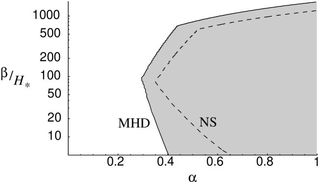
By fixing the temperature at which EWPT happens at $100$ GeV, eqs. (63) and (67) are functions of $\alpha$, $\beta$ and $f$; the LISA (expected) sensitivity in $h_{0}^{2}\Omega_{\rm gw}$ clearly depends only on frequency $f$ and it is roughly $10^{-11}$ at $0.1$ mHz, $10^{-12}$ at $1$ mHz and $10^{-11}$ at $10$ mHz (see [1] for the LISA sensitivity curve). Figure 1 shows the values of $\alpha$ and $\beta$ for which there exists at least a range of frequency in which the signals (63) and (67) are above the sensitivity of LISA. Clearly large values of $\alpha$, i.e. strong transitions, are favoured. Notice that too large values of $\beta/H_{*}$ are disfavoured, because in such cases the characteristic frequency (62) is too high for LISA. Notice the effect of the MHD corrections, which substantially enhance the detectability of the signal mostly at small values of $\beta/H_{*}$, because in such cases the characteristic frequency (62) is quite below the sensitivity window of LISA.

Furthermore, we should keep in mind that tangled magnetic fields act themselves as a source of GWs [13]. Assuming that magnetic fields are in equipartition with the turbulent velocity field, this source should enhance the expected GW signal by a factor of two in all the frequency range over which equipartition is established (see eq. (21)).

7 Conclusions

In this paper we investigated the characteristics of the GW signal sourced by turbulence in the early universe. We extended previous work on the subject by considering the effects on the turbulence energy spectrum of a continuous stirring power and of magnetic fields. In the first part of our work we derived a suitable parameterization for the turbulent energy spectrum in the case of a continuous stirring power with and without external magnetic fields. Interestingly we found that the MHD turbulent spectrum can be written in the same form as the Navier-Stokes ones upon a simple rescaling of only two parameters. Our treatment is original and may find applications which go beyond the aims of this paper. Following the approach of Kosowsky et al. [4], who consider only Kolmogorov type of turbulence, we used our formulation to determine the characteristics of the GW signal produced by cosmological turbulence with a more general energy spectrum. In the Kolmogorov case we found minor discrepancies with the result reported in [4]. Deviations from the Kolmogorov spectrum may have relevant consequences for the GW signal. Indeed, since the modified spectra are generally less steep than the Kolmogorov’s, these deviations will result in a stronger signal at high frequencies. Furthermore, our analysis may allow to extract valuable informations about the nature of the turbulence source and the presence of primordial magnetic fields from the GW background power spectrum which may be measured by forthcoming experiments.

We applied our results to estimate the GW expected signal for two possible kind of sources. In sec. 5 we considered GW production by neutrino inhomogeneous diffusion according to the mechanism proposed in Ref. [6]. We showed that a detectable signal can be produced only if the amplitude of the lepton number fluctuations is close to unity over a wide range of wavenumbers. This possibility is not unreasonable as active-sterile neutrino oscillations or some models of leptogenesis based on the Affleck-Dine scenario can indeed give rise to domains with opposite lepton number. Although we argued that the former scenarios can hardly give rise to GW signal detectable by LISA, the latter scenario offers more promising observational perspectives.

Finally in sec. 6 we considered GW production by turbulence at the end of a first order phase transition. In the absence of strong magnetic fields no substantial deviations have to be expected from the results of Ref. [4] based on the assumption of a Kolmogorov turbulence spectrum. In the case of the EWPT the GW signal may be above the LISA planned sensitivity only if the transitions is very strong with large bubble wall velocities. This may be achieved in next to minimal extensions of the supersymmetric standard model [5]. A more favorable situations may be obtained if strong magnetic fields were present at the end of the transition. This is actually to be expected in the case of the EWPT if it is first order [9]. We showed that in this case the signal can be strongly enhanced with respect to the non-magnetic case and be detectable by LISA if bubble wall velocity was not too much smaller than unity. Similar consideration may apply to other physical situations like, for example, during reheating at the end of inflation. These results open new perspectives for a successful detection of GWs backgrounds produced in the early universe.

Acknowledgments

The authors thanks G. Falkovich for useful comments. D. G. thanks the CERN theory division for ospitality during the last writing of this paper.

Appendix

Computation of the spectrum $h_{0}^{2}\Omega_{\rm gw}(f)$

In this appendix we work out the detailed computation of the relic spectrum $h_{0}^{2}\Omega_{\rm gw}(f)$ in the three cases $\gamma<2/3$, $\gamma\simeq 2/3$ and $\gamma>2/3$, along the strategy described in section 4.

If $\gamma<2/3$ eq. (29) becomes

$$\langle\>h_{ij}({\bf k},t_{*})\>h_{ij}^{*}({\bf k}^{\prime},t_{*})\>\rangle\simeq\frac{27\cdot 64\sqrt{2}\>\pi^{7}(Gw)^{2}}{(2-3\gamma)V^{2}}\>\Delta t_{*}\>\>u_{S}^{4}\>k_{S}^{2/3-\gamma}\>\delta^{3}({\bf k}-{\bf k}^{\prime})\>k^{-20/3+\gamma}\;,$$ (68)

which in real space reads

$$\langle\>h_{ij}({\bf x},t_{*})\>h_{ij}({\bf x},t_{*})\>\rangle \simeq \frac{27\cdot 4\sqrt{2}\>\pi^{2}\>(Gw)^{2}}{2-3\gamma}\>\Delta t_{*}\>\>u_{S}^{4}\>k_{S}^{2/3-\gamma}\int^{k_{D}}_{k_{S}}k^{-14/3+\gamma}dk$$ (69)

$$= \frac{27\cdot 4\sqrt{2}\>\pi^{2}\>(Gw)^{2}}{2-3\gamma}\>\Delta t_{*}\>\>u_{S}^{4}\>k_{S}^{-3}\int^{k_{D}}_{k_{S}}\left(\frac{k}{k_{S}}\right)^{-\frac{11-3\gamma}{3}}\frac{dk}{k}\;.$$ (70)

Changing variable from the turbulent scale $k$ to the characteristic frequency $f$ (see eq. (34)), we have

$$\langle\>h_{ij}({\bf x},t_{*})\>h_{ij}({\bf x},t_{*})\>\rangle\simeq\frac{81\cdot 8\sqrt{2}\>\pi^{2}\>(Gw)^{2}}{(2-3\gamma)(4+3\gamma)}\>\Delta t_{*}\>\>u_{S}^{4}\>k_{S}^{-3}\int^{f_{D}}_{f_{S}}\left(\frac{f}{f_{S}}\right)^{-\frac{2(11-3\gamma)}{4+3\gamma}}\frac{df}{f}\;,$$ (71)

where $f_{S}\equiv f_{k_{S}}$ is the characteristic frequency of the largest length scale. The characteristic amplitude squared is thus

$$h_{c}^{2}(f,t_{*})=\frac{81\cdot 4\sqrt{2}\>\pi^{2}\>(Gw)^{2}}{(2-3\gamma)(4+3\gamma)}\>\Delta t_{*}\>u_{S}^{4}\>k_{S}^{-3}\left(\frac{f}{f_{S}}\right)^{-\frac{2(11-3\gamma)}{4+3\gamma}}\;.$$ (72)

The characteristic amplitude squared measured today at a frequency $f$ (see eq. (39)) is

$$h_{c}^{2}(f,t_{0})\simeq\frac{3.3\times 10^{-18}}{(2-3\gamma)(4+3\gamma)}\>u_{S}^{4}\left[\frac{\Delta t_{*}}{H_{*}^{-1}}\right]\left[\frac{k_{S}}{H_{*}}\right]^{-3}\left[\frac{T_{*}}{\rm MeV}\right]^{-2}\left[\frac{g_{*}}{10.75}\right]^{-2/3}\left(\frac{f}{f_{S}}\right)^{-\frac{2(11-3\gamma)}{4+3\gamma}}\;,$$ (73)

where we used $Gw=H_{*}/(2\pi)$ and both frequencies $f$ and $f_{S}$ have been redshifted. By means of eqs. (40) and (44) we finally have the spectrum, eq. (41).

The above computations can be easily generalized to the $\gamma>2/3$ case:

$$\langle\>h_{ij}({\bf k},t_{*})\>h_{ij}^{*}({\bf k}^{\prime},t_{*})\>\rangle\simeq\frac{27\cdot 64\sqrt{2}\>\pi^{7}(Gw)^{2}\>(11-3\gamma)}{(3\gamma-2)(13-6\gamma)V^{2}}\>\Delta t_{*}\>\>u_{S}^{4}\>k_{S}^{4/3-2\gamma}\>\delta^{3}({\bf k}-{\bf k}^{\prime})\>k^{-\frac{2(11-3\gamma)}{3}}\;,$$ (74)

i.e.

$$\langle\>h_{ij}({\bf x},t_{*})\>h_{ij}({\bf x},t_{*})\>\rangle\! \!\simeq\! \!\frac{27\cdot 4\sqrt{2}\>\pi^{2}(Gw)^{2}\>(11-3\gamma)}{(3\gamma-2)(13-6\gamma}\>\Delta t_{*}\>\>u_{S}^{4}\>k_{S}^{-3}\int^{k_{D}}_{k_{S}}\left(\frac{k}{k_{S}}\right)^{-\frac{13-6\gamma)}{3}}\frac{dk}{k}$$ (75)

$$\!\simeq\! \!\frac{81\cdot 8\sqrt{2}\>\pi^{2}(Gw)^{2}\>(11-3\gamma)}{(3\gamma-2)(13-6\gamma)(4+3\gamma)}\>\Delta t_{*}\>\>u_{S}^{4}\>k_{S}^{-3}\int^{f_{D}}_{f_{S}}\left(\frac{f}{f_{S}}\right)^{-\frac{2(13-6\gamma)}{4+3\gamma}}\frac{df}{f}$$

$$h^{2}_{c}(f,t_{*})\! \!\simeq\! \!\frac{81\cdot 4\sqrt{2}\>\pi^{2}(Gw)^{2}\>(11-3\gamma)}{(3\gamma-2)(13-6\gamma)(4+3\gamma)}\>\Delta t_{*}\>\>u_{S}^{4}\>k_{S}^{-3}\>\left(\frac{f}{f_{S}}\right)^{-\frac{2(13-6\gamma)}{4+3\gamma}}\;.$$ (76)

The characteristic amplitude measured today is

$$h_{c}^{2}(f)\simeq\frac{3.3\times 10^{-18}\>(11-3\gamma)}{(3-\gamma)(13-6\gamma)(4+3\gamma)}\>u_{S}^{4}\left[\frac{\Delta t_{*}}{H_{*}^{-1}}\right]\left[\frac{k_{S}}{H_{*}}\right]^{-3}\left[\frac{T_{*}}{\rm MeV}\right]^{-2}\left[\frac{g_{*}}{10.75}\right]^{-2/3}\left(\frac{f}{f_{S}}\right)^{-\frac{2(13-6\gamma)}{4+3\gamma}}\;,$$ (77)

which, combined with eq. (40), gives eq. (42).

Looking at eq. (31) we see that the intermediate case $\gamma\simeq 2/3$ is formally the same as $\gamma<2/3$ case, with the replacements $\gamma\to 2/3$ and $\frac{3}{2-3\gamma}\to 1$, and with an extra logarithmic factor. The present-day observable are thus

$$h_{c}^{2}(f)\simeq 1.8\times 10^{-19}\>u_{S}^{4}\left[\frac{\Delta t_{*}}{H_{*}^{-1}}\right]\left[\frac{k_{S}}{H_{*}}\right]^{-3}\left[\frac{T_{*}}{\rm MeV}\right]^{-2}\left[\frac{g_{*}}{10.75}\right]^{-2/3}\left(\frac{f}{f_{S}}\right)^{-3}\log{\frac{f}{f_{S}}}$$ (78)

and the spectrum given in eq. (43).

As a cross-check, notice that the $\gamma\simeq 2/3$ case is also equal to the $\gamma<2/3$ one, again modulo proper replacements and the logarithmic factor. The present-day observable computed in the two ways are equal.

References

- [1] M. Maggiore, “Gravitational wave experiments and early universe cosmology,” Phys. Rept. 331, 283 (2000) [arXiv:gr-qc/9909001].
- [2] “LISA: Laser Interferometer Space Antenna for the detection and observation of gravitational waves, pre-phase-A report, December 1995,” MPQ-208; K. Danzmann, “LISA - an ESA cornerstone mission for a gravitational wave observatory,” Class. Quant. Grav. 14, 1399 (1997).
- [3] M. Kamionkowski, A. Kosowsky and M. S. Turner, “Gravitational radiation from first order phase transitions,” Phys. Rev. D 49, 2837 (1994) [arXiv:astro-ph/9310044].
- [4] A. Kosowsky, A. Mack and T. Kahniashvili, “Gravitational radiation from cosmological turbulence,” Phys. Rev. D, in press (2002) [arXiv:astro-ph/0111483].
- [5] R. Apreda, M. Maggiore, A. Nicolis and A. Riotto, “Supersymmetric phase transitions and gravitational waves at LISA,” Class. Quant. Grav. 18, L155 (2001) [arXiv:hep-ph/0102140]; “Gravitational waves from electroweak phase transitions,” Nucl. Phys. B 631, 342 (2002) [arXiv:gr-qc/0107033].
- [6] A. D. Dolgov and D. Grasso, “Generation of cosmic magnetic fields and gravitational waves at neutrino decoupling,” Phys. Rev. Lett. 88, 011301 (2002) [arXiv:astro-ph/0106154].
- [7] A. D. Dolgov and D. P. Kirilova, J. Moscow Phys. Soc. 1, 217 (1991).
- [8] P. Di Bari, “Amplification of isocurvature perturbations induced by active-sterile neutrino oscillations,” Phys. Lett. B 482, 150 (2000) [arXiv:hep-ph/9911214].
- [9] G. Baym, D. Bödeker and L. McLerran, “Magnetic fields produced by phase transition bubbles in the electroweak phase transition,” Phys. Rev. D 53, 662 (1996).
- [10] D. Grasso and H. R. Rubinstein, “Magnetic fields in the early universe,” Phys. Rept. 348, 163 (2001) [arXiv:astro-ph/0009061].
- [11] W. Frost and T. T. Moulden, “Handbook of Turbulence,” Plenum Pub. Corp. (1977); D. Bernard, “Turbulence for (and by) amateurs,” arXiv:cond-mat/0007106.
- [12] D. Biskamp, “Nonlinear Magnetohydrodynamic,” Cambridge, Cambridge University Press (1993).
- [13] R. Durrer, P.G. Ferreira and T. Kahniashvili, “Tensor microwave anisotropies from a stochastic magnetic field,” Phys. Rev. D 61 043001 (2000) [arXiv:astro-ph/9911040].
- [14] J. Adams, U. H. Danielsson, D. Grasso and H. Rubinstein, “Distortion of the acoustic peaks in the CMBR due to a primordial magnetic field,” Phys. Lett. B 388, 253 (1996) [arXiv:astro-ph/9607043]; K. Jedamzik, V. Katalinic and A. V. Olinto, “A Limit on Primordial Small-Scale Magnetic Fields from CMB Distortions,” Phys. Rev. Lett. 85, 700 (2000) [arXiv:astro-ph/9911100]; A. Mack, T. Kahniashvili and A. Kosowsky, “Vector and Tensor Microwave Background Signatures of a Primordial Stochastic Magnetic Field,” Phys. Rev. D 65, 123004 (2002) [arXiv:astro-ph/0105504].
- [15] J. Bernstein, “Kinetic Theory In The Expanding Universe,” Cambridge, USA, University Press (1988).
- [16] A. D. Dolgov, “Neutrinos in cosmology,” to be published in Phys. Rept. [arXiv:hep-ph/0202122].
- [17] A. D. Dolgov, “NonGUT baryogenesis,” Phys. Rept. 222, 309 (1992).
- [18] M. S. Turner, E. J. Weinberg and L. M. Widrow, “Bubble nucleation in first order inflation and other cosmological phase transitions,” Phys. Rev. D 46, 2384 (1992).
- [19] A. Riotto and M. Trodden, “Recent progress in baryogenesis,” Ann. Rev. Nucl. Part. Sci. 49, 35 (1999) [arXiv:hep-ph/9901362].