An investigation of gravitational lens determinations of ${\rm H_{o}}$ in quintessence cosmologies

Abstract

There is growing evidence that the majority of the energy density of the universe is not baryonic or dark matter, rather it resides in an exotic component with negative pressure. The nature of this ‘quintessence’ influences our view of the universe, modifying angular diameter and luminosity distances. Here, we examine the influence of a quintessence component upon gravitational lens time delays. As well as a static quintessence component, an evolving equation of state is also considered. It is found that the equation of state of the quintessence component and its evolution influence the value of the Hubble’s constant derived from gravitational lenses. However, the differences between evolving and non-evolving cosmologies are relatively small. We undertake a suite of Monte Carlo simulations to examine the potential constraints that can be placed on the universal equation of state from the monitoring of gravitational lens system, and demonstrate that at least an order of magnitude more lenses than currently known will have to be discovered and analysed to accurately probe any quintessence component.

1 Introduction

The searches for supernovae at cosmological distances have proved very successful, providing evidence that, while topologically flat, the majority of energy in the Universe is in the form of an exotic component with negative pressure (Riess et al. 1999; Perlmutter et al. 1999). The recent identification of a supernova at $z=1.7$ (Riess et al. 2001)  has provided further weight to these claims (Turner & Riess 2001), which suggest that this component may differ from the classical cosmological constant $\Lambda$. Termed ‘quintessence’, or more colloquially ‘dark energy’, this has an equation of state of the form $P=w\rho$, where $P$ is the pressure and $\rho$ the density. A $w<-\frac{1}{3}$ opposes the action of gravity and drives the cosmological expansion to accelerate. Linder (1988a; 1988b) has examined the physical nature of various quintessence components; with $w=0$ equating to non-relativistic matter (dust), $w=\frac{1}{3}$ being radiation and $w=-1$, a classical cosmological constant. More exotic components are; massless scalar fields $w=1$, cosmic string networks $w=-\frac{1}{3}$, and two-dimensional topological defects $w=-\frac{2}{3}$. As well as the supernova programs, other approaches, such as gravitational lensing statistics (Cooray & Huterer 1999), geometrical probes of the ${\rm Ly_{\alpha}}$ forest (Hui, Stebbins & Burles 1999) and galaxy distributions (Yamamoto & Nishioka 2001), and classical angular-size redshift tests (Lima & Alcaniz 2001), will provide complementary probes of the universal equation of state.

The value of the quintessence component, $w$, influences our view of the universe, modifying the various distances used in mapping the cosmos. This paper concerns itself with the influence of $w$ on angular diameter distances, especially in relation to the determination of the Hubble’s constant from the measurement of time delays in gravitational lens systems. Unlike local determinations of Hubble’s constant (e.g. Freedman et al. 2001), the cosmological nature of gravitational lenses means that they are more sensitive to the underlying cosmological parameters. Section 2 briefly covers the basic formulae for generalized angular diameter distances in quintessence cosmologies, while in Section 3 we consider the influence of $w$ on the determination of $H_{o}$ from lensed systems. Section 4 extends this analysis to simple models of an evolving quintessence component. In Section 5 a series of Monte Carlo simulations are undertaken to estimate the efficacy of this approach in probing the cosmological equation of state, while in Section 6 we speculate on the possability that current observations of gravitational lens systems may suggest that $w<-1$. The conclusions of this study are presented in Section 7.

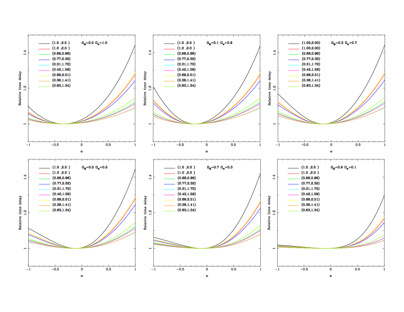
Figure 1: The relative time delays for several flat cosmologies as a function of the equation of state, $w$. Each curve is is for the lowest value of the time delay (the redshift of the lens-source pair is given in brackets). Each panel presents a different combination of $\Omega_{m}$ and $\Omega_{w}$; note that $w=0$ corresponds to a universe composed entirely of matter in all cases.

2 Generalized Angular Diameter Distances

While there has been a resurgence in quintessence cosmology, the generalized cosmological equations for such universes were presented more than a decade ago by Linder (1988a;1988b), including a generalized form of the Dyer-Roeder equation for the evolution of a bundle of rays traveling from a distant source (Dyer & Roeder 1973). Expressing the angular diameter distance as $D=(c/H_{o})r$, the generalized beam equation is given by

$$\ddot{r}+\left[\frac{3+q(z)}{1+z}\right]\dot{r}+\sum_{w}\frac{3r(1+w)\alpha_{w}(z)\Omega_{w}(z)}{2(1+z)^{2}}=0$$ (1)

where $\Omega_{w}(z)$ is the density, in units of the critical density $\rho_{c}(z)$, of a contributor to the total energy-density of the universe with an equation of state $w=P/\rho$, and where $P$ is its pressure and $\rho$ is its density. This is given by

$$\Omega_{w}(z)\equiv\frac{\rho_{w}(z)}{\rho_{c}(z)}=\Omega_{w}(0)(1+z)^{3(1+w)}\left[\frac{H_{o}}{H(z)}\right]^{2}$$ (2)

where $\Omega_{w}(0)$ is the contribution of this component to the present energy-density budget at the present epoch, and the critical density is given by $\rho_{c}(z)=3H(z)^{2}/8\pi G$. Here, $H(z)$ is a generalized form of the Hubble parameter and is given by;

$$H(z)=H_{o}\left[\sum_{w}\Omega_{w}(0)(1+z)^{3(1+w)}-K(1+z)^{2}\right]^{\frac{1}{2}}$$ (3)

where $K=\Omega_{o}-1$, and $\Omega_{o}\equiv\Omega(0)=\sum_{w}\Omega_{w}(0)$, is related to the overall curvature of the universe. $q(z)$ is a generalized form of the deceleration parameter and is given by

$$q(z)=\frac{1}{2}\frac{\sum_{w}\Omega_{w}(0)(1+3w)(1+z)^{1+3w}}{\sum_{w}\Omega_{w}(0)(1+z)^{1+3w}-K}$$ (4)

Finally, Equation 1 also contains the parameter $\alpha_{w}(z)$ which represents how much of the fluid lies in the beam and influences the the evolution of a ray bundle. For a universe containing matter, the solution to Equation 1 with $\alpha_{0}(z)=1$ represents the classic Dyer-Roeder ‘filled beam’ distance, while $\alpha_{0}(z)=0$ is the ‘empty beam’ distance (Dyer & Roeder 1973).

Figure 2: The top panel presents the angular diameter distance of a source at $z$ for an observer at $z=0$, for the evolutionary $w$ models discussed in the text. The thick lines correspond to universes with $w_{0}=-1$, while the thin line represents $w_{0}=-0.7$. The solid line represents a non-evolving model with $w_{1}=0$, while the dashed lines evolve as $w_{1}=0.2$ and the dot-dashed lines as $w_{1}=0.4$. The lower panel presents the percentage difference between the evolving models and non-evolving model.

When solving Equation 1, the boundary conditions need to be defined. These are

$$r(z_{0},z_{0})=0,$$ (5)

$$\left.\frac{dr(z_{0},z)}{dz}\right|_{z=z_{0}}=(1+z_{0})^{-1}\left[\frac{H_{o}}{H(z)}\right]$$ (6)

Equation 1 was integrated using a Runge-Kutta scheme (the rksuite package from www.netlib.org) and compared to both analytic results and the minimum angular extent redshifts in quintessence cosmologies as tabulated in Lima & Alcaniz (2000); excellent agreement was found. Throughout this work, filled-beam distances $\alpha_{w}(z)=1$ are employed.

Figure 3: As for Figure 2, but for an observer at $z=1.0$.

3 Gravitational lens time delays

Refsdal (1964) was the first to note that cosmological parameters could be determined from the measurement of a time delay between the relative paths taken by light though a gravitational lens system. Since the discovery of multiply-imaged quasars, this has become the goal of a number of monitoring campaigns (e.g. Cohen et al. 2000; Oscoz et al. 2001; Patnaik & Narashima 2001), although these analyses are frustrated by degeneracies in the derived mass models. The cosmological model simply enters the determination of Hubble’s constant;

$$H_{o}\Delta t\propto\frac{r_{ol}r_{os}}{r_{ls}}$$ (7)

where $r_{ij}$ are the normalized angular diameter distances between and observer $(o)$, lens $(l)$ and source $(s)$, and $\Delta t$ is the measured time delay between an image pair.

Giovi & Amendola (2001) examined the influence on a quintessence component on gravitational lens time delays and the determination of Hubble’s constant. Their analysis, however, was mainly concerned with the influence of the clumping of material and the dependence on $H_{o}$ of whether distances are empty-beam or full-beam. Here, a different approach is considered; Solving Equation 1, Equation 7 is evaluated for a range of quintessence components. For the study, the redshifts of the lens and source in seven gravitational lens systems that are favourable for time delay measures were considered [Table 2 in Giovi & Amendola (2001), Q0957+561 and B1608+656], plus two fiducial redshift pairs of $(z_{l}=1.5,z_{s}=2.5)$ and $(z_{l}=1.0,z_{s}=2.0)$. While there are currently no lensed systems with established time delays at these particular redshifts, there are several potential systems; e.g. the quadruple lens H1413+117 at a redshift of 2.55, with a lens redshift, established from prominent absorption features, at $\sim 1.5$ and HE1104-1805 at a redshift of 2.31 and an estimated lens redshift of $z\sim 1$. It is assumed throughout that the universe is flat, $\Omega_{m}+\Omega_{w}=1$.

$\Omega_{m}$	$\Omega_{w}$	$w_{min}$
0.0	1.0	-0.33
0.1	0.9	-0.22
0.3	0.7	-0.15
0.5	0.5	-0.12
0.7	0.3	-0.10
0.9	0.1	-0.09

Table 1: The minima for the curves in Figure 1 for the various cosmologies under consideration.

Figure 1 presents the results of this analysis; six panels are presented, each for a different combination of $\Omega_{m}$ and $\Omega_{w}$. A greyscale-coded line for each redshift pair is presented. The abscissa presents the equation of state parameter, $w$, while the ordinate presents the relative time-delay; this represents the change in the time delay for a fixed Hubble’s constant. Conversely, this is the relative value of $H_{o}$ for a system with a fixed time delay. Each curve is normalized to the minimum value of the time delay. The relative time delay depends quite strongly on the value of $w$, with the $(z_{l}=1.5,z_{s}=2.5)$ possessing changes of $\sim 40\%$ at $w=1$ as compared to $w\sim 0$, although, for the observed lensing systems, the same range in $w$ produces a change of $\sim 10\%$ in the same quantity. Interestingly, for a fixed combination of $\Omega_{m}$ and $\Omega_{w}$, all the curves, irrespective of the redshift of the lens and source possess a minimum at the same value of $w$. The location of the minimum is tabulated in Table 1.

At present, the general analytic solution to Equation 1 is quite complex (Giovi & Amendola 2001) and it is difficult to further analyze the minimum seen in Figures 1. For one case, where $\Omega_{m}=0.0$ and $\Omega_{w}=1.0$, however, analytic solutions for the relative angular diameter distance are straight forward. As the overall curvature is flat, the angular diameter distance between us and a distant source is

$$D_{A}(z)=\frac{D_{c}(z)}{1+z}$$ (8)

where $D_{c}(z)$ is the comoving distance and is given by

$$D_{c}(z)=\frac{c}{H_{o}}\int_{o}^{z}\frac{dz^{\prime}}{E(z^{\prime})}$$ (9)

where $E(z)=\Omega_{w}(0)(1+z)^{\frac{3}{2}(1+w)}$. Again, as the overall cosmology is flat, the angular diameter distance between the source and the lens is given by;

$$D_{A}(z_{1},z_{2})=\frac{1}{1+z_{2}}\left[D_{c}(z_{2})-D_{c}(z_{1})\right]$$ (10)

With this, the relative time delays for differing values of $w$ is seen to be:

$$H_{o}\left[z_{1},z_{2}\right]\propto\frac{1}{1+z_{1}}\frac{2}{1+3w}\left[\frac{(1-(1+z_{1})^{f})(1-(1+z_{2})^{f})}{(1+z_{1})^{f}-(1+z_{2})^{f}}\right]$$ (11)

where $f=-\frac{1}{2}(1+3w)$. This function possesses a minimum at $w=-\frac{1}{3}$, which is independent for the redshift pairs under consideration, as seen in Figure 1.

The preceding section has considered arbitrary combinations of cosmological parameters. Here, the impact of the choice of $w$ on the estimation of $H_{o}$ in the favoured cosmological model with $\Omega_{m}=0.3$ and $\Omega_{w}=0.7$ (top right panel in Figure 1) is examined in more detail. Often, a cosmological model where $\Omega_{m}=1$ is choosen when estimating $H_{o}$ from time delays, which is equivalent to considering $w=0$ in Figure 1. An accelerating cosmology, as suggested from the cosmological supernovae programs, requires $w<-\frac{1}{3}$. It is interesting to note that in this cosmology, the minimum $H_{o}$ occurs at $w=-0.15$ (Table 1) the values of $H_{o}$ derived at $w=0$ or $w=-\frac{1}{3}$ will be very similar. Considering more negative values of $w$, adopting classical cosmological constant, with $w=-1$ results in $H_{o}$ values that are $\sim 5\%$ different to the all matter case ($w=0$). For several combinations of redshifts, however, (including the chosen fiducial points) more substatial differences of $\sim 12-15\%$ in the determined value of $H_{o}$. Considering $w<-1$ results in more significant discrepancies, a point that will be returned to later.

4 Evolving quintessence

One interesting aspect of quintessence cosmology is that, unlike classical $\Omega_{m},\Omega_{\Lambda}$ cosmologies, it is possible that the equation of state $w$ may vary over the cosmic history of the universe. Typically, a linear model where $w(z)\sim w_{0}+w_{1}z$ has been adopted (e.g. Goliath et al. 2001). In the following analysis, it is assumed that $\Omega_{m}=0.3$ and $\Omega_{w}=0.7$, consistent with the recent supernova experiments (Riess et al. 1999; Perlmutter et al. 1999) results. Four models for the evolution of $w$ are adopted [taken from Linder (2001)], namely, $(w_{0},w_{1})=(-0.7,0.2),(-0.7,0.4),(-1.0,0.2)$ and $(-1.0,0.4)$. As the cosmology is flat, we follow the approach outlined in Equations 8, 9 and 10, with

$$E(z)=\sqrt{(1+z)^{3}\Omega_{m}+f_{w}(z)\Omega_{w}}$$ (12)

and

$$f_{w}(z)=\exp\left[3\int_{o}^{z}\frac{1+w(z^{\prime})}{1+z^{\prime}}dz^{\prime}\right].$$ (13)

$z_{l}$	$z_{s}$	$(-1.0,0.2)$	$(-1.0,0.4)$	$(-0.7,0.2)$	$(-0.7,0.4)$
1.50	2.50	0.997	1.003	1.012	1.043
1.00	2.00	1.000	1.005	1.010	1.029
0.68	0.96	1.003	1.007	1.007	1.015
0.77	2.32	1.001	1.005	1.009	1.026
0.31	1.72	1.002	1.005	1.005	1.012
0.42	1.59	1.002	1.006	1.006	1.014
0.89	2.51	1.000	1.005	1.010	1.030
0.36	1.41	1.002	1.006	1.005	1.012
0.63	1.34	1.002	1.006	1.008	1.017

Table 2: The ration of the time delay (or conversely $H_{0}$) for the cosmologies with linearly evolving quintessence. The first two columns are the lens and source redshifts, while the next four columns present the time delays for $(w_{0},w_{1})$. Those with $w_{0}=-1$ are normalized with respect to $(-1.0,0.0)$, while those with $w_{0}=-0.7$ are normalized with respect to $(-0.7,0.0)$.

Figures 2 and 3 present the angular diameter distance in these evolving models for an observer at $z=0$ and $z=1$ respectively. It is interesting to note that for an observer at redshifts greater than zero the fractional difference between the angular diameter distances for an evolving and non-evolving quintessence component does not converge to zero as $z_{s}\rightarrow z_{l}$, rather, as seen in the lower box of Figure 3, they converge to a non-zero value. This seems somewhat counter-intuitive given the convergence of distances for an observer at redshift zero (Figure 2). Employing Equation 10 and setting $z_{2}=z_{1}+\Delta z$, the angular diameter distance becomes;

$$D_{A}(z_{1},z_{1}+\Delta z)\sim\frac{\Delta z}{1+z_{1}}\left.\frac{dD_{c}(z)}{dz}\right|_{z=z_{1}}$$ (14)

where $\Delta z\ll 1+z_{1}$. Therefore, the asymptotic ratio of the angular diameter distance in a non-evolving cosmology, with a constant $w_{0}$, and one where $w(z)=w_{0}+zw_{1}$, as $z_{2}\rightarrow z_{1}$ simply becomes;

$$\frac{D_{A}(z_{1},w_{0})}{D_{A}(z_{1},w(z))}=\sqrt{\frac{\Omega_{m}(1+z_{1})^{3}+\Omega_{w}(1+z_{1})^{3(1+w_{0})}}{\Omega_{m}(1+z_{1})^{3}+\Omega_{w}g(z_{1})}},$$ (15)

where

$$g(z)=\exp\left\{3(zw_{1}+(1+w_{o}-w_{1})\log[1+z])\right\}.$$ (16)

With the values under consideration in Figure 3, this is precisely the asymptote seen.

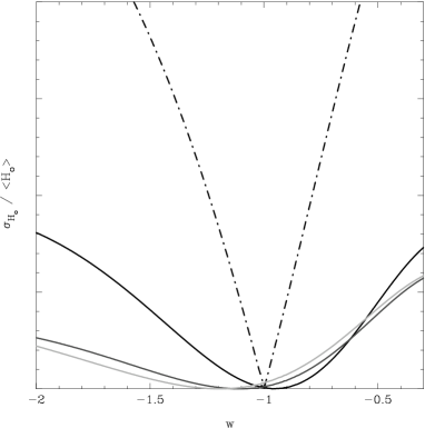
Figure 4: The cosmological minimization function, $\sigma_{H_{o}}/\left<H_{o}\right>$, versus the quintessence equation of state for the chosen fiducial cosmology and a sample of one hundred gravitational lens system. The dot-dash line represents the ideal case with no noise; as can be seen this is zero at $w=-1$. The black line assumes an uncertainty in the time-delay and lens modeling of 5%, the lighter curve of 10% and the lightest 15%. A DC component has been subtracted from these latter curves.

As seen from Equation 7, the cosmological component of the measure of Hubble’s constant is dependent upon a combination of angular diameter distances. Table 2 presents the relative values in the measured Hubble’s constant for the linear evolution models described above, for the lens systems in Section 3. The largest changes are seen in the first two rows which represent fiducial models; these possess the highest lens redshifts in the sample. For the observed lens system, it is clear that the evolving quintessence models do differ from non-evolving models, this difference is not substantial, being typically less than a few percent for evolution models with $w_{1}=0.4$.

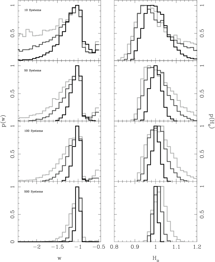
Figure 5: The results of the Monte Carlo simulations of the determination of the quintessence equation of state and Hubble’s constant from the measurement of samples of gravitational lens time delays. The black line assumes an uncertainty in the time-delay and lens modeling of 5%, the lighter curve of 10% and the lightest 15%

5 Monte Carlo Simulations

How many lensed systems are required before firm limits can be made? To address this question a number of Monte Carlo simulations were undertaken with a population of lensed sources, assuming that for each a time delay could be determined to a specified accuracy. For real lensed systems, additional uncertainty is introduced from the lens modeling. Here, however, it is assumed that the lens modeling introduces no systematic uncertainty and that the random error is taken into account as an additional source of uncertainty in the time delay.

A number of programs have examined the relative statistics of gravitational lensing (e.g. Kochanek 1993a; 1993b; Williams 1998; Falco et al. 1998; Helbig et al. 1999). The complex analyses in these studies go beyond this paper and a more straight forward approach was adopted; this was to examine the distribution of source and lens redshift pairs in the CASTLES database (Muñoz et al. 1998). This is seen to be a scatter plot of sources between redshifts 1 and 4, with lenses between 0.2 and 1.1. Source $(z_{s})$ and lens $(z_{l})$ redshifts where, therefore, selected randomly in these range, but ensuring that $z_{s}>4z_{l}-2.2$. This cut ensures that lens and sources are always reasonably separated in redshift space.

In choosing a background cosmology, a fiducial model with $\Omega_{m}=0.3$ and $\Omega_{w}=0.7$ with a $w=-1$ and $H_{o}=1$ was employed. In an ideal universe, where there are no measurement errors and where gravitational lens models can be uniquely determined, the analysis of a sample of systems may still produce a distribution of $H_{o}$ values, as an incorrect choice of cosmological parameters, including the quintessence equation of state $w$, influences differently each system (e.g. Figure 1). In this ideal universe, however, all one would need to do is to vary the cosmological parameters until all systems yielded the same value for the Hubble constant. In this way, not only would $H_{o}$ be measured, but the underlying cosmology would be determined as well.

In the real universe, however, the influence of measurement uncertainties needs to be considered. Instead of obtaining a unique value of Hubble’s constant, one could vary the cosmological parameters such that the dispersion in the resultant $H_{o}$’s are minimized. An example of this for a population of one hundred gravitational lens systems is given in Figure 4; note that the function that is minimized is $\sigma_{H_{o}}/\left<H_{o}\right>$ as it is the fractional dispersion of the results that is of interest. The dot-dashed line is the ideal universe case, where there are no sources of uncertainty, which possesses a minimum value (of zero) at the chosen fiducial value. The solid curves represent varying values of noise in the determination of the time delay, the black being 5% noise, grey 10% and light grey 15% noise. Clearly this function broadens as more noise is added, and the minimum is not necessarily at the fiducial value of $w$.

	10	50	100	500
5%	(-3.52,-0.14)	(-1.39,-0.78)	(-1.25,-0.89)	(-1.10,-0.92)
10%	(-4.41,-0.13)	(-3.85,-0.15)	(-1.70,-0.54)	(-1.23,-0.92)
15%	(-4.45,-0.13)	(-4.52,-0.13)	(-4.09,-0.14)	(-1.48,-0.88)
5%	(0.91,1.30)	(0.97,1.07)	(0.98,1.04)	(0.99,1.02)
10%	(0.88,1.39)	(0.92,1.36)	(0.95,1.13)	(0.99,1.05)
15%	(0.87,1.42)	(0.92,1.42)	(0.93,1.39)	(0.99,1.10)

Table 3: The 95% confidence intervals for $w$ (upper values) and $H_{o}$ (lower values) for the Monte Carlo samples described in the text. The sample sizes are given across the top of the table, and each row is for an assumed error in the determination of the time delay. Note that in calculating these confidence intervals, outlying points with $w>0$ have been neglected so that they represent the width of the distribution.

Figure 5 presents the results of undertaking this procedure for various samples of gravitational lens systems. The left panel presents the probability distribution for the quintessence equation of state $w$ while the right hand panel is the corresponding distribution in Hubble’s constants; note that all the distributions have been normalized to a peak value of one. The top row is for a sample of ten gravitational lens systems, akin to the situation today, followed by 50, 100 and 500 systems. Ten thousand realizations were undertaken for each sample size. Each line on the plot corresponds to a different level of uncertainty in the gravitational lens time delay as outlined in the previous paragraph. Clearly today, where there are but a handful of gravitational lens systems for which we have determined the time delay, with overall uncertainties exceeding 5-10%, then the resultant Hubble’s constant and $w$ that can be derived from the sample are unlikely to accurately represent the underlying values.

Table 3 presents the 95% confidence interval for the estimation of $w$ and $H_{o}$ for the various samples. Increasing the sample size greatly improves the situation, although even with 500 lenses and 15% noise, the values of $w$ and $H_{o}$ are not strongly constrained. One is led to conclude, therefore, that a large sample of lenses with very accurately determined time delays and lens models is required to significantly determine the the underlying cosmological parameters. Given the observational effort in such a task, other approaches to probing the cosmological equation of state are likely to prove more fruitful. Given this, the analysis was not extended to consider the smaller influences of quintessence evolution (see Section 4).

6 Do current lens systems suggest $w<-1$?

Can the current observations of time delays in gravitational lens systems tell us anything about the equation of state of the quintessence component? In recent years, dedicated monitoring of a number of lensed systems has provided accurate $(\sim 10-20\%)$ time delay determinations (e.g. Fassnacht et al. 1999; Koopmans et al. 2000). An examination of the Hubble’s constant derived from such studies reveals that, typically, it is less than the value determined from local studies, even accounting for standard cosmological differences (e.g. Impey et al. 1998; Koopmans et al. 2001; Winn et al. 2002). This very question was also recently addressed by Kochanek (2002) who suggests that this discrepancy is potentially due to galaxies possessing concentrated dark matter halos with a constant mass-to-light ratios, at odds with expectations from cold dark matter structure models. Here, an alternative solution is considered.

Examining the panel in Figure 1 corresponding to an $\Omega_{m}=0.3,\Omega_{w}=0.7$ cosmology, it is apparent that choosing $\Omega_{m}=1$ (equivalent to setting $w=0$) results in almost the lowest possible determination of $H_{o}$. Considering a cosmology with a classical cosmological constant ($w=-1$) increases the determined value of $H_{o}$ by $\sim 5-20\%$ (dependent upon the source and lens redshifts), but as noted above, the currently determined values still tend to lie below the 72${\rm km/s/Mpc}$ derived locally (Freedman et al. 2001). Assuming that the gravitational lens models are correct, one way to reach concordance between the two approaches is that $w<-1$; such a conclusion is consistent with the recently derived limit of $w<-0.85$ from an analysis of a combination of cosmic microwave background, high redshift supernovae, cluster abundances and large scale structure data (Wang et al. 2000; Bean & Melchiorri 2001). While tantalizing, however, it must be conceded that the current differences in the approaches are not statistically significant, especially given the relatively large uncertainty in the modeling of gravitational lens mass distributions (see, for example, the range of $H_{o}$ values obtained from the modeling of PG 1115+080; Kochanek 2002). Given a large sample of gravitational lens systems, however, the determination of a systematic difference in the derived Hubble’s constant could be made.

7 Conclusions

This paper has investigated the role of a quintessence component on angular diameter distances, specifically their influence on the determination of Hubble’s constant from the measurement of a time delay in multiply imaged quasars.

For flat universes, with an unevolving quintessence component, its seen that, for a gravitational lens system in which the time delay has been measured, the resultant Hubble’s constant is dependent upon the value of the equation of state parameter $w$. Interestingly, the dependence of the determined value of the Hubble’s constant as a function of $w$ possesses a minimum which is independent on the lens and source redshift.

Several models of evolving quintessence were also examined, consisting of a linear evolution of the equation of state with redshift. The cosmologies resulted in significantly different forms of the angular diameter distance. Hence, our view of the cosmos would be different in the various cosmologies. When considering the specific combination of angular diameter distances that constitute the cosmological contribution to the gravitational lensing determination of Hubble’s constant, it is seen that the resulting variations between cosmologies is very small, a matter of only a few percent, relative to an unevolving case with the same present day constitution.

A number of Monte Carlo simulations of the determination of Hubble’s constant and the quintessence equation of state, $w$, were undertaken to explore the efficacy of this approach. These revealed that the present situation with only a handful of lensed systems does not allow an accurate determination of the cosmic equation of state, and that at least an order of magnitude more lenses are truly required to provide a reasonably robust determination of the underlying cosmology. The next generation of all-sky surveys are presently underway (e.g. Sloan Digital Sky Survey) or are being planned (e.g. VISTA, PRIME), and these datasets will greatly increase the number of lensed quasars available for monitoring studies. Cooray & Huterer (1999) estimate that $\sim 2000$ lensed quasars will be identified from the SDSS database alone, and a much larger number can be expected from the deeper VISTA and PRIME surveys. The number of these sources amenable for follow-up monitoring campaigns will naturally be much smaller, but one can confidently expect a sample of several hundred systems to eventually become available. However, given the effort required to first find such systems, as well as monitor them to determine the time delays and the modeling procedure, it is likely that $w$ will be first determined using one of the other various techniques currently being proposed. We conclude, therefore, that gravitational lens time delays are likely to prove poor probes of the universal equation of state.

References

- [sdrer] Bean, R., Melchiorri, A., 2001, astro-ph/0110472
- [Caldwell et al. 1998] Caldwell R. R., Dave R., Steinhardt P. J., 1998, Ap&SS, 261, 303
- [Cohen et al. 2000] Cohen A. S., Hewitt J. N.,Moore C. B., Haarsma D. B., 2000, ApJ, 545, 578
- [Cooray & Huterer 1999] Cooray A. R., Huterer D., 1999, ApJ, 513, L95
- [Dyer & Roeder 1973] Dyer C. C., Roeder R. C., 1973, ApJ, 180, L31
- [Falco et al. 1998] Falco E. E., Kochanek C. S., Munoz J. A., 1998, ApJ, 494, 47.
- [Fassnacht et al. 1999] Fassnacht C. D., Pearson T. J., Readhead A. C. S., Browne I. W. A., Koopmans L. V. E., Myers S. T., Wilkinson P. N., 1999, ApJ, 527, 498
- [Freedman et al.(2001)] Freedman, W. L. et al. 2001, ApJ, 553, 47
- [Futamase & Yoshida 2001] Futamase T., Yoshida S., 2001, Progress of Theoretical Physics, 105, 887
- [Giovi & Amendola 2001] Giovi F., Amendola L., 2001, MNRAS, 325, 1097
- [Goliath et al. 2001] Goliath, A., Amanulah, R., Astier, P., Goobar, A., Pain, R., 2001, A&A, 380, 6
- [Helbig et al. 1999] Helbig P., Marlow D., Quast R., Wilkinson P. N., Browne I. W. A., Koopmans L. V. E., 1999, A&AS, 136, 297.
- [Impey et al. 1998] Impey C. D., Falco E. E., Kochanek C. S., Lehár J., McLeod B. A., Rix H.-W., Peng C. Y., Keeton C. R., 1998, ApJ, 509, 551.
- [Kochanek 1993] Kochanek C. S., 1993a, ApJ, 419, 12
- [Kochanek 1993] Kochanek C. S., 1993b, ApJ, 417, 438
- [Kochanek 1993] Kochanek C. S., 2002, astro-ph/0204043
- [koop] Koopmans, L. V. E. et al., 2001, PASA, 18, 179
- [Koopma] Koopmans, L. V. E., de Bruyn, A. G., Xanthopoulos, E., & Fassnacht, C. D. 2000, A&A, 356, 391
- [Lewis & Ibata 2001] Lewis G. F., Ibata R. A., 2001, MNRAS, 324, L25
- [Lima & Alcaniz 2000] Lima J. A. S., Alcaniz J. S., 2000, A&A, 357, 393
- [Linder 1988] Linder E. V., 1988a, A&A, 206, 190
- [Linder 1988] Linder E. V., 1988b, A&A, 206, 175
- [Linder 2001] Linder E. V., 2001, astro-ph/0108280
- [Hui et al. 1999] Hui L., Stebbins A., Burles S., 1999, ApJ, 511, L5
- [Mörtsell et al. 2001] Mörtsell E., Gunnarsson C., Goobar A., 2001, ApJ, 561, 106
- [Muñoz et al. 1998] Muñoz J. A., Falco E. E., Kochanek C. S., Lehár J., McLeod B. A., Impey C. D., Rix H.-W., Peng C. Y., 1998, Ap&SS, 263, 51
- [Oscoz et al. 2001] Oscoz A., Alcalde D.,Serra-Ricart M., et al., 2001, ApJ, 552, 81
- [Patnaik & Narasimha 2001] Patnaik A. R., Narasimha D., 2001, MNRAS, 326, 1403
- [Peacock et al. 2001] Peacock J. A., Cole S.,Norberg P., et al., 2001, Nature, 410, 169
- [Perlmutter et al. 1999] Perlmutter S., Aldering G., Goldhaber G., et al., 1999, ApJ, 517, 565
- [Refsdal 1964] Refsdal S., 1964, MNRAS, 128,307
- [Riess et al. 1998] Riess A. G., Filippenko A. V., Challis P., et al., 1998, AJ, 116, 1009
- [Riess et al. 2001] Riess A. G. et al. 2001, ApJ, 560, 49
- [Schechter et al. 1997] Schechter P. L., Bailyn C. D., Barr R., et al., 1997, ApJ, 475, L85.
- [Turner & Riess 2001] Turner, M. S., Riess, A. G., 2001, astro-ph/0106051
- [Wang et al. 2000] Wang L., Caldwell R. R., Ostriker J. P., Steinhardt P. J., 2000, ApJ, 530, 17.
- [Williams 1998] Williams L. L. R., 1998, New Astronomy Review, 42, 81
- [Winn] Winn, J. N., Kochanek, C. S., McLeod B. A., Falco, E. E., Impey, C. D., Rix H.-W., 2002, astro-ph/0201551
- [Yamamoto & Nishioka 2001] Yamamoto K., Nishioka H., 2001, ApJ, 549, L15