The Mg-$\sigma$ Relation and the Genesis of Early-Type Galaxies

Abstract

Available data on the magnesium - velocity dispersion (Mg-$\sigma$) relation for $\sim$2000 early-type galaxies is collected and compared. As noted previously, the Mg residuals from a fitted line are roughly Gaussian near the mean but have an asymmetric blue tail, probably from subpopulations of relatively young stars. We define statistics for scatter and asymmetry of scatter in the Mg dimension and find impressive uniformity among data sets. We construct models of galaxy formation built to be as unbiased as possible toward the question of the importance of mergers in the formation of early type galaxies. The observational constraints (Mg-$\sigma$ width, asymmetry, and mean Mg strength, plus mean age and width of abundance distribution) are severe enough to eliminate almost all of models. Among the casualties are: models with merger rates proportional to $(1+z)^{n}$ with $n>0$, models that assume early formation followed by recent drizzling of new stars, merger-only models where the number of mergers exceeds $\approx$80, merger-only models with less than $\approx$20 mergers, and models with a cold dark matter power spectrum even with biasing included. The most successful models were those with merger probability constant with time, with the number of mergers needed to form the galaxy around 40. These models are characterized by mean light-weighted ages of 7-10 Gyr (consistent with spectroscopic studies), a narrow abundance distribution, and a lookback time behavior nearly indistinguishable from passive evolution of old stellar populations.

Galaxies : Abundance — Galaxies : Elliptical — Galaxies : Evolution — Galaxies : formation — Galaxies : Stellar content.

1 Introduction

The process of formation of early-type galaxies is still largely unknown. Under study since Larson (1975), the choice between formation of elliptical galaxies by a single brief collapse or via merging is still disputed in the astronomical literature.

Some properties of early-type galaxies are very uniform, suggesting a homogeneous and probably ancient origin. Elliptical and S0 galaxies have smooth light profiles and very low gas and dust content, like overgrown globular clusters. As a class, they display scaling relations such as a tight Fundamental Plane (FP: Djorgovsky & Davies (1987); Dressler et al. (1987)) among the variables luminosity, size, and velocity dispersion, a narrow Mg-$\sigma$ relation between integrated starlight absorption line strength and velocity dispersion Bender et al. (1993); Ziegler & Bender (1997), and an orderly color-magnitude relation. Many authors note that elliptical galaxies nearby and at intermediate redshift have properties consistent with old, passively evolving systems (Stanford et al., 1998; van Dokkum & Franx, 1996; Kelson et al., 1997; Ellis et al., 1997; Kodama & Arimoto, 1997; Kodama et al., 1998; Bender et al., 1998; van Dokkum et al., 1998).

Confusingly, there is also a great deal of evidence that favors a messier, ongoing formation process for early-type galaxies. Some galaxy mergers are caught in the act (Toomre, 1977) with the theoretical expectation that the remnant will soon relax to resemble an elliptical, with an exponential light profile. The tails, ripples, shells, and other morphological aftereffects of merging are seen in many nearby elliptical galaxies (Schweizer et al., 1990; Schweizer & Seitzer, 1992; Goudfrooij et al., 2001; Bardelli et al., 2002; Markevitch et al., 2002). Measurements of the integrated stellar absorption features compared with stellar population models indicate light-weighted mean ages for the near-nuclear regions of elliptical galaxies that range from ancient through a median of $\sim$7 Gyr to a few that appear less than 1 Gyr old (González, 1993; Worthey, 1997; Terlevich & Forbes, 2002). Young stellar populations are much brighter than old populations, so that a relatively modest burst of young stars may be able to skew the mean age of an essentially old galaxy to appear much younger than a mass-weighted mean age, but the presence of any youthful subpopulation contradicts the uniform-and-old hypothesis.

With this paper we attempt to bring clarity to the issue. To simplify, we consider only the relation between the central velocity dispersion $\sigma$ and the strength of the integrated stellar Mg and MgH features around 5100Å. The advantages of this relation are its distance independence and its small scatter (Jørgensen et al., 1996; Bender et al., 1998). One disadvantage is that age and metallicity both have a similar effect on the Mg strength (Worthey, 1994; Forbes et al., 2001; Colless et al., 1999): an older galaxy has a stronger Mg feature, but Mg strength can also be increased by Mg abundance. It is clear that the origin of the relation itself is primarily one of abundance: larger galaxies have more heavy elements. Intrinsic scatter exits in the $Mg_{2}$-$\sigma_{0}$ relation ($\sigma_{0}$ refers to an aperture-corrected central velocity dispersion). This scatter is not correlated with the appearance of the galaxies, with the degree of velocity anisotropy, with their environment (Dressler et al., 1987; Burstein et al., 1990), or with deviation of the objects within (or perpendiculiar) to the FP. Bender et al. (1993) intrepreted this as a combination of age and/or metallicity differencies among ellipticals with similar luminosity, and Colless et al. (1999) find that both mean age and metallicity vary, probably in a correlated manner with younger-appearing galaxies tending to be somewhat more metal-rich. This correlation is also seen with Balmer-metal indicators (Worthey, Trager, & Faber, 1995; Terlevich & Forbes, 2002)

The residuals of $Mg_{2}$ have a Gaussian core, but the galaxies with weaker $Mg_{2}$ at given $\sigma_{0}$ form a tail. That is, the residual distribution is skewed with an excess of Mg-weak galaxies (Bender et al., 1993). This is suggestive of late star formation: A youthful galaxy will have weak Mg strength from the presence of bright, hot stars with weak Mg strength and will appear as a low outlier.

We test two opposing hypotheses. In both cases, the Mg-$\sigma$ relation is a mass-abundance correlation. In the “ancient formation” hypothesis, elliptical galaxies formed at the epoch of galaxy formation at high redshift (we assume $z_{f}$=5). The Mg-$\sigma$ relation was put in place at that time. Furthermore, the symmetric portion of the scatter was put in place at formation. (We could be even more extreme and suggest that the asymmetric part of scatter was also imprinted at formation by an asymmetric abundance distribution, but the implication of this is trivial: except for the effect of passive stellar evolution the Mg-$\sigma$ relation would remain unchanged back to $z_{f}$.) In the “ancient formation” hypothesis, mergers, as inconsequential as possible, cause occasional bursts of star formation that drive a few galaxies to weak Mg strength and cause the asymmetry of the observed relation. In the “maximum merger” hypothesis, the underlying Mg-$\sigma$ relation is very tight, and all scatter, symmetric or not, is caused by merging events (convolved with observational error).

To compare these two views, we first collect and analyze published Mg-$\sigma$ data sets of E and S0 galaxies from field, group, and cluster environments. We use these data to find robust statistics to help us evaluate the expected asymmetrical scatter. In $\S$3 we describe special-purpose models that predict Mg-$\sigma$ relations given input parameters such as the number of mergers and gas fraction of each merger. Results are discussed in $\S$4, and a summary of conclusions is given in $\S$5.

2 Observational Data

We analyse the Mg-$\sigma$ relation in 7 different data sets for E and S0 galaxies. There are three Lick/IDS system Mg indices: Mg₁, Mg₂, Mg$b$ (Worthey et al., 1994), plus the variant $<$Mg${}_{2}>$ index introduced by Davies et al (1987), and defined by :

$$<Mg_{2}>=0.6\,Mg_{2}+0.4\,Mg^{{}^{\prime}},\ {\rm with}\ Mg^{{}^{\prime}}=0.03+2.1\,Mg_{1}-62Mg^{4}_{1}.$$

$<$Mg${}_{2}>$ uses the additional signal available in Mg₁ to improve the precision of the Mg₂ index. There does not appear to be any substantial mismatch between $<$Mg${}_{2}>$ and Mg₂ definitions in ultimate index behavior, although differences are detectable (Trager et al., 1998). We summarize the literature data that we collected with a few words and a table of characteristics in table 1.

Data set 1 is a subset of data extracted from Trager et al. (1998), it consists of 256 galaxies observed at the Lick Observatory between 1972 and 1984. Average errors for Mg₂, Mgb, and $<$Mg${}_{2}>$ indices were 0.008 mag, 0.23 Å, 0.006 mag, respectively. For velocity dispersion the error is less than 10 $\%$. The advantage of these data is that they define the Lick system and are very homogeneous. The disadvantage is that no aperture corrections for distance have been included. This appears to have no measureable consequence (see Table 1).

Data set 2 is part of the ENEAR database from Bernardi et al (1998) that does not overlap any other samples. It is separated into 3 data sets according to whether the galaxies were assigned to field, group or cluster environments. Measurements of $\sigma$ are accurate to 5%-13%, Mg₂ to 0.005-0.011 mag.

Data set 3: Dressler et al. (1991) have presented 136 cluster and group elliptical and S0 galaxies in the direction of the large-scale streaming flow attributed to the great attractor. The typical errors are 0.05 dex for log$\sigma$ and 0.017 mag for Mg₂.

Data set 4: The 528 galaxies available with the Mg₂ index in Hudson et al. (2001) are from 56 galaxy clusters. Uncertainties on log$\sigma$ are 5% and 0.009 mag for Mg₂.

Data set 5: We culled almost 150 galaxies taken from the EFAR data (Wegner et al., 1999). The whole sample is much larger but we considered only those galaxies that had errors of 7% or less in $\sigma$. Errors for Mg₂ were 0.015 mag and for Mg$b$ 0.37 Å.

Data set 6: Davies et al (1987) (the 7 Samurai) computed $\sigma$ and lines indices for 600 galaxies from all environments. The scatter of measurements indicates an uncertainty of 10 % and 0.009 mag for $\sigma$ and $<$Mg${}_{2}>$, respectively. We use an updated 7 Samurai data set kindly provided by D.Burstein (1999, private communication).

Data set 7: This data set of 650 ellipticals and SO galaxies was extracted from Prugniel & Simien (1996). It is a literature compilation with considerable overlap with the 7 Samurai data set but with different procedures for homogenization. The data are in $\sigma$ (same error: 10%), and in Mg₂ (error : 0.009 mag).

With the data in hand we then sought suitable statistics to describe the scatter and asymmetry of the residuals from a linear fit to the data. The linear fit itself was tried several ways. A line fit via least-squares method was too sensitive to the presence of outliers. Even when we clipped the outliers in a rejection loop we judged that the resulting line was too unstable. Finally, we binned the data in log$\sigma$, found the median Mg index value of each bin, weighted each datum by $\frac{1}{\sqrt{N}}$, and performed a least-squares fit on the array of medians. This method is outlier-insensitive and very stable. Unless specified otherwise in this paper, the fit was computed only for $150<\sigma<320$ km/s; medium-sized and large galaxies. In table 1, we report the number of galaxies really used for our fit.

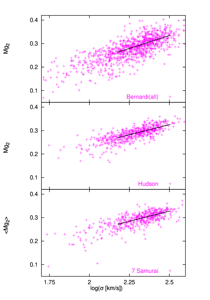
Figure 1: Observational Mg₂-$\sigma$ relation for 3 of our data sets : Bernardi (all galaxies), Hudson, and 7 Samurai. The median fit line is shown within the limits we chose for calculating statistics : 150 $<\,\sigma\,<$ 320 km/s.

There is a small amount of systematic drift among the data sets. The Table 1 column marked “Mg 300” is the value of the Mg index fit for $\sigma=300$ km/s. This quantity is 0.327 $\pm$ 0.039 for Mg₂, 5.1 $\pm$ 0.085 for Mg$b$, and 0.333 $\pm$ 0.007 for $<$Mg${}_{2}>$, averaged over the data sets. For illustration, we plot three data sets and the computed median line in Figure 1.

Once the line was fit, we sought statistics to characterize the distribution of Mg index residuals in terms of both width and asymmetry. For width, the standard deviation has the advantage that everyone is familiar with it, but it is quite sensitive to outliers due to its $x^{2}$ dependence. We prefer the average deviation, or ADev (mean absolute deviation). It is an estimator of width less sensitive to outliers than the standard deviation. It is defined by :

$$ADev(x_{1}\dots x_{N})=\frac{1}{N}\,\sum^{N}_{j=1}|x_{j}-\bar{x}|$$

but in this case we substitute the median-fit line value $x_{med}$ for $\bar{x}$.

For measuring asymmetric tails we need another statistic. We considered the skewness, a dimensionless number which describes only the shape of the distribution. We take the usual definition :

$$Skew(x_{1}\,\dots\,x_{N})=\frac{1}{N}\sum^{N}_{j=1}\left(\begin{array}[]{c}\frac{x_{j}-\bar{x}}{\sigma}\end{array}\right)^{3}$$

where $\sigma$ is the distribution’s standard deviation. A positive value of skewness signifies a distribution with an asymmetric tail extending out towards more positive $x$. A negative value signifies a distribution whose tail extends out towards more negative $x$. We expect a negative skewness if galaxies scatter preferentially toward weaker Mg index values.

Because we wish to be outlier-insensitive, we also define an “average deviation ratio” (ADR) of the ADevs above and below the fitted line, that avoids the $x^{3}$ dependence of traditional skewness. Since we expect more weak-lined galaxies than strong-lined, we define the ADR so that it will be greater than one for asymmetries toward weak Mg index values.

$$ADR_{Mg_{2}}=\frac{\sum^{N}_{j=1}|x_{j}-\bar{x}|_{``bottom^{\prime\prime}}}{\sum^{N}_{j=1}|x_{j}-\bar{x}|_{``top^{\prime\prime}}}$$

The results are summarised in table 1. The value of the standard deviation is relatively stable at 0.027 $\pm$ 0.003 for Mg₂, 0.474 $\pm$ 0.052 for Mg$b$ and 0.035 $\pm$ 0.003 for $<$Mg${}_{2}>$ among the different data sets. The skewness is definitely negative, between -0.052 and -1.75 for Mg₂, around -0.7 for Mg$b$ and -4. for $<$Mg${}_{2}>$, but shows too much scatter to be very useful.

The ADev and ADR are more stable due to their relative insensitivity to outliers (ADev: 0.0206$\pm$ 0.0014, 0.346 $\pm$ 0.032, 0.02 $\pm$ 0.001 and ADR: 1.265 $\pm$ 0.058, 1.105 $\pm$ .12, 1.7 $\pm$ 0.09 for Mg₂, Mg$b$, $<$Mg${}_{2}>$ respectively). So for the rest of our study we prefer focusing on these two statistics.

Bender et al. (1993) noted that Mg residuals could be described by a Gaussian core with extra galaxies at weak Mg strength. The width of this Gaussian core is also of crucial interest for the “ancient formation” hypothesis because it represents the amount of scatter imprinted on the Mg-$\sigma$ relation at formation. In order to find its width from the various data sets, we compute the number of galaxies within bins of 0.01 mag in both Mg₂ and $<$Mg${}_{2}>$ residual, and within bins of 0.1 Å in Mg$b$.

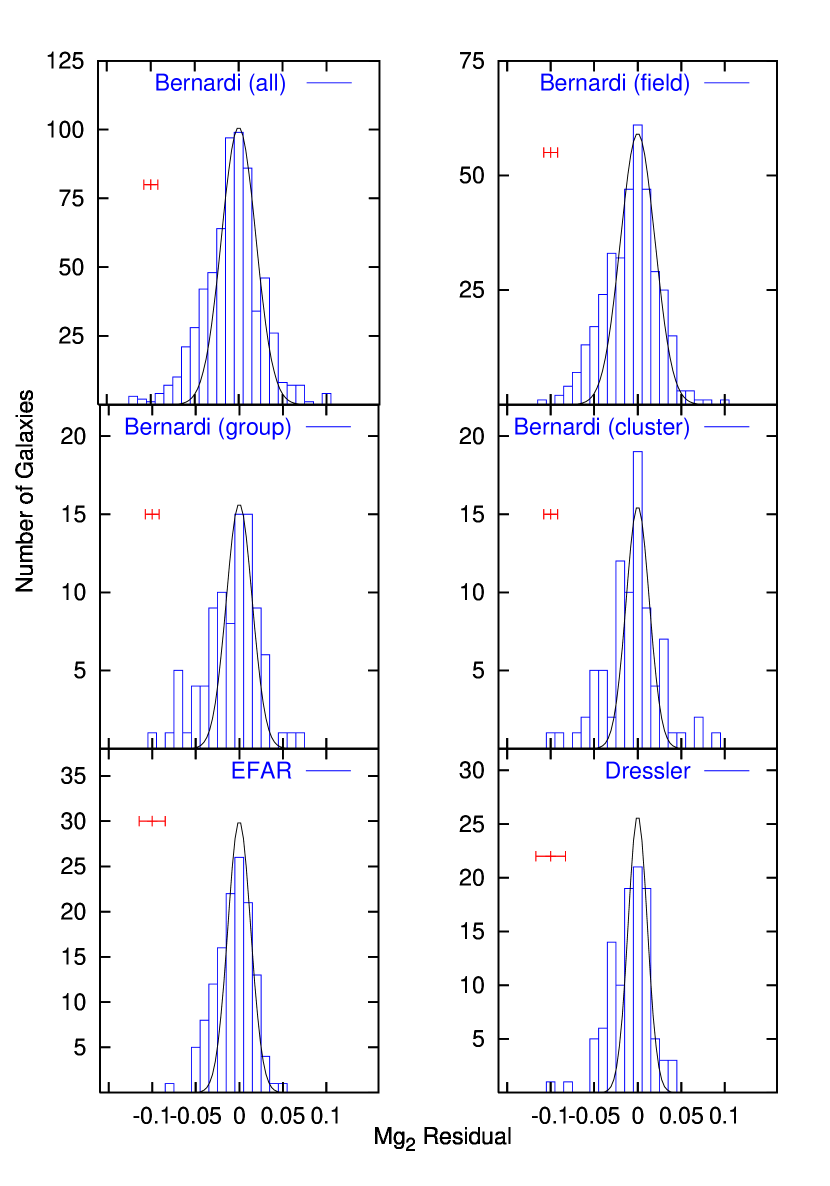
Figure 2: Number of galaxies versus Mg₂ residual. The curve is the Gaussian fit for the peak at zero. The bar at top left shows the typical uncertainty on the measurements.

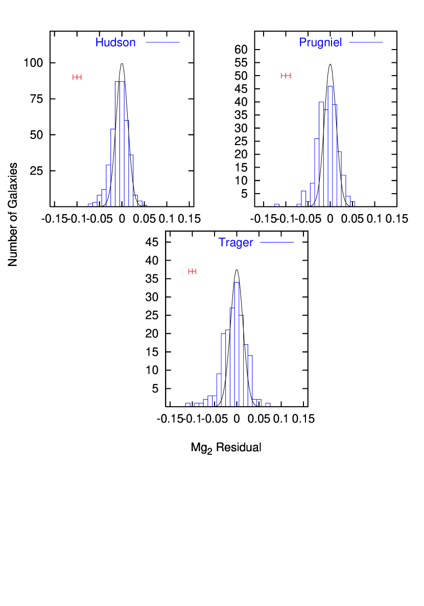
Figure 3: Number of galaxies versus Mg₂ residual. The curve is the Gaussian fit for the peak at zero. The bar at top left shows the typical uncertainty on the measurements.

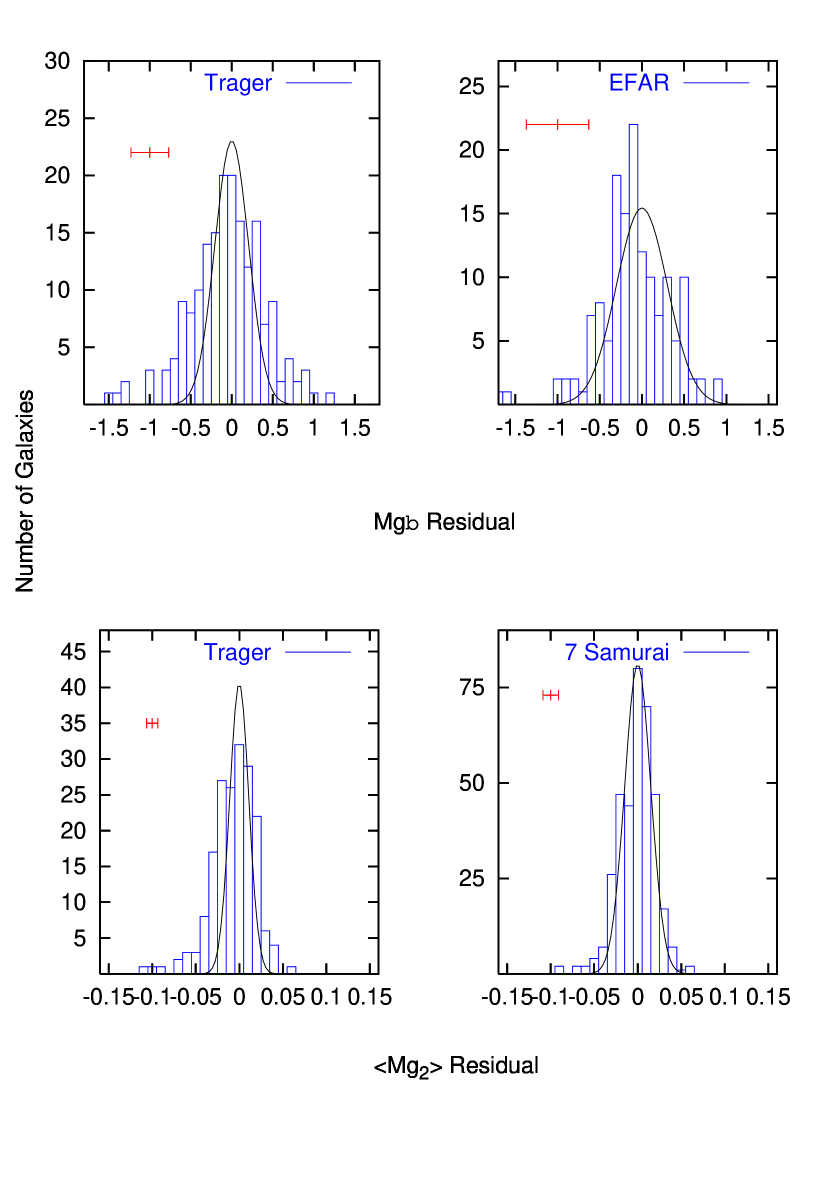
Figure 4: Number of galaxies versus Mg$b$ (or $<$Mg${}_{2}>$) residual. The curve is the Gaussian fit for the peak at zero. The bar at top left shows the typical uncertainty on the measurements.

We fit with a Gaussian the principal peak from Mg residual distributions, weighting by $\sqrt{N}$ in each bin (See fig 2, fig 3 and fig 4). These fits yielded widths that were very close for all the data sets except for the EFAR and Dressler et al. (1991) samples. But these are also the samples with the largest observational errors, and we conclude that this is why the fitted Gaussians are more broad. On average, we found $\sigma_{g}$ equal to 0.0147 $\pm$ 0.002 for Mg₂, and 0.013 $\pm$ 0.002 for $<$Mg${}_{2}>$. Because of the difference of units, $\sigma_{g}$ for the Mg$b$ index is broader: $\sigma_{g}=0.25\pm 0.05$.

All data sets give remarkably similar characteristics. We see no statistically significant difference in width or asymmetry among E and S0 galaxies in different environments (field, group or cluster). Also note that our method of line-fitting yields Mg₃₀₀ field-group-cluster offsets even smaller than those computed by Bernardi et al (1998) from the same data.

For the remainder of the paper, we prefer the ADev and ADR statistics for providing the first-order discriminant for the synthetic Mg-$\sigma$ diagrams, whose generation discuss in the following section.

3 Merger Models

In order to understand the effects of galaxy merging on the scatter in the Mg-$\sigma$ relation we constructed hybrid models that contain simple galaxy merging trees and rudimentary chemical evolution but a relatively rigorous treatment of the effect of stellar ages on Mg feature strength. The aim of the resultant Monte Carlo simulation is to make a synthetic Mg-$\sigma$ diagram where the stretch along the $\sigma$ axis is heuristic and approximate but where the scatter in the Mg strength direction is modeled well. Also, relative zeropoint changes in Mg strength are reliable; for example, the weakening of Mg feature strength with increasing lookback time is well modeled (if one can assume that ellipticals today were also ellipticals in the past).

There are several simplifying assumptions in the models. Chemical enrichment proceeds in a schematic way. A mass-[Mg/H] relation is assumed, and a pre-merger galaxy fragment is assumed to have the [Mg/H] appropriate for its mass. Upon merging, newly incorporated gas is assumed to become stellar with an [Mg/H] derived from the post-merger mass. Only the gas enriches in this way; the stellar portion of the merger fragments retain their original abundance. Using this scheme, the Mg abundance is driven toward higher values in larger galaxies, as is observed. This is one of the more heuristic elements of the models, the chief intent being to produce a spread of galaxy Mg strengths. Almost any mechanism that accomplishes this is sufficient for the purposes of this exercise since it is the spread of Mg strength from stellar age effects that is under study, not the origin of the relationship itself.

The choice of [Mg/H] rather than [Fe/H] is mandated by observation. At high metallicities, elliptical galaxies are seen to have approximately constant Fe-feature strength as a function of velocity dispersion (Trager et al., 1998). Mg-feature strengths increase with velocity dispersion, and the tight relation between the two variables is the cause of this investigation. Scaled-solar stellar population models predict that both species should increase together with increasing metallicity (e.g. Worthey (1994)), so it is mostly Mg (and presumably other light metals) that drives the increase of abundance in the largest galaxies. Since the deep Mg feature at 5100Å is the easily measured, [Mg/H] becomes our abundance parameter. We choose [Mg/H]$\approx$0.6 for the most extreme $\sigma$=390 km/s, $M$=10¹⁴ M_⊙ giant ellipticals, and [Mg/H]$\approx$0 for $\sigma$=150 km/s, $M$=5.7$\times$10¹² M_⊙ smaller elliptical galaxies.

The relation between velocity dispersion and mass is a projection of the fundamental plane. Specifically, a relation in Kappa-space from Bender et al. (1992) was chosen to pass from compact ellipticals through giant ellipticals, namely $\kappa_{2}=2.2+0.2\kappa_{1}$. This translates to a rough relation between galaxy mass and velocity dispersion: $M=0.0322\sigma_{0}^{-3.394}$. This relation is used in the simulations to translate mass (the fundamental variable in the simulations) to velocity dispersion. The artificiality of this relation does not affect the conclusions of this paper, and its simplicity allows us to explore the stellar population effects caused by complex merger histories.

The part of the models that is not approximate is the treatment of the stellar populations. Quick interpolation tables were summarized from Worthey (1994) models using both the original Yale/VandenBerg evolution and the Bertelli et al. (1994) isochrones for younger ages. Lookups can be done for $V$ luminosity and the three Mg indices. The simulation delivers a galaxy formed at several (or many) epochs. These are collected as a list of ages, masses, and [Mg/H] abundances. Index strengths are computed as a function of age and [Mg/H] and weighted by $V$ luminosity computed as a function of age, [Mg/H], and mass for each tagged star parcel within the final galaxy assemblage.

The main parameters in the models are four. The number of equal-mass merger fragments that will eventually combine to form the final galaxy, the fraction of the final galaxy that formed at the redshift of formation $z=z_{f}$, the gas fraction of the mergers $F_{\rm gas}=m_{\rm gas}/m_{\rm total}$, and a probablility envelope that is either flat with time between $z_{f}$ and $z=0$ or is proportional to $(1+z)^{n}$, where $n$ is a free parameter.

Other parameters control cosmology, set $z_{f}$, set the number of galaxies to be generated and their mass range, introduce artificial scatter into the computed Mg-$\sigma$ relation, and provide for extra (or not as much) Mg enrichment at each star formation episode.

Throughout this paper we adopt $H_{0}=60\,km/s/Mpc$, $\Omega=.2$, $\Omega_{R}=.8$, $\Omega_{\Lambda}=0$. With these parameters, the universe is 13.8 Gyr old, and $z_{f}=5$ corresponds to a lookback time of 12.3 Gyr. We flagged galaxies that experienced star formation within the last 50 Myr as “star forming” and they are omitted from all statistical calculations. As the majority of data sets feature the Mg₂ index, we use this index for all of the following discussion even though the models predict all index varieties.

4 Merger Model Discussion

4.1 Basic Model Behavior

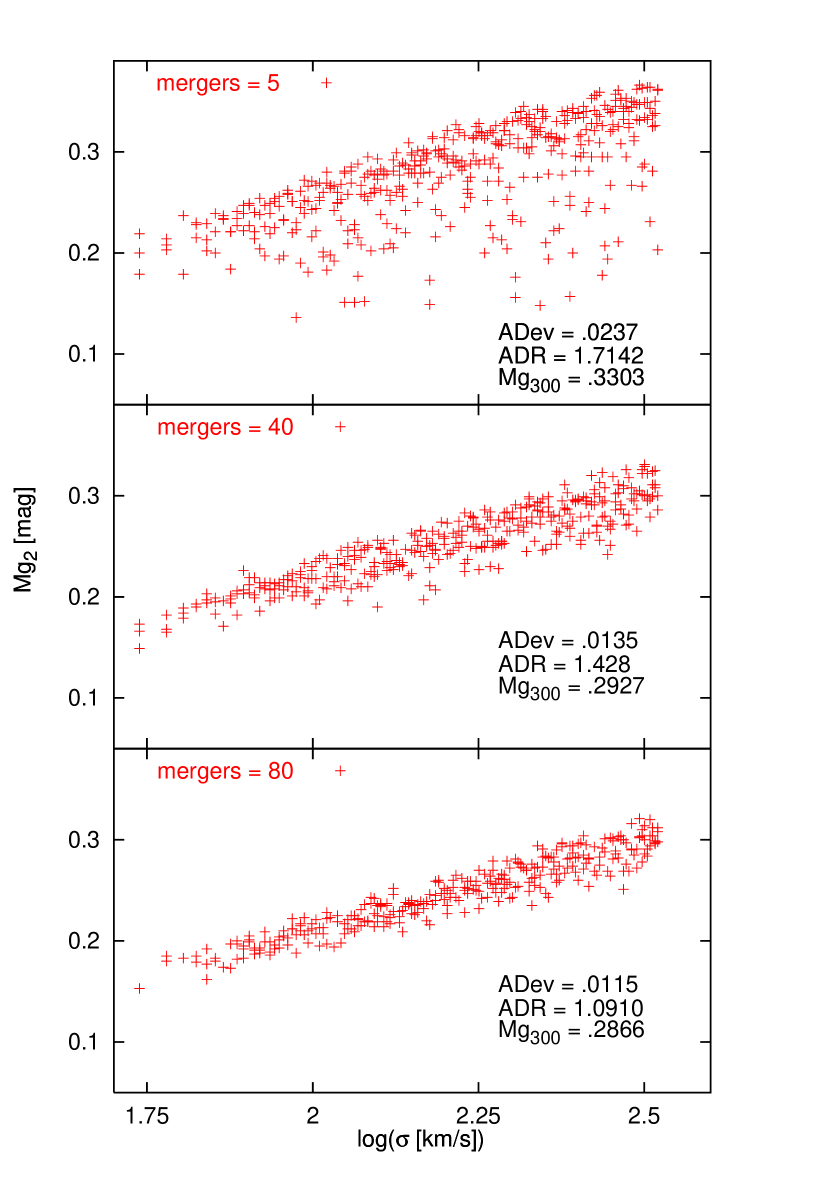
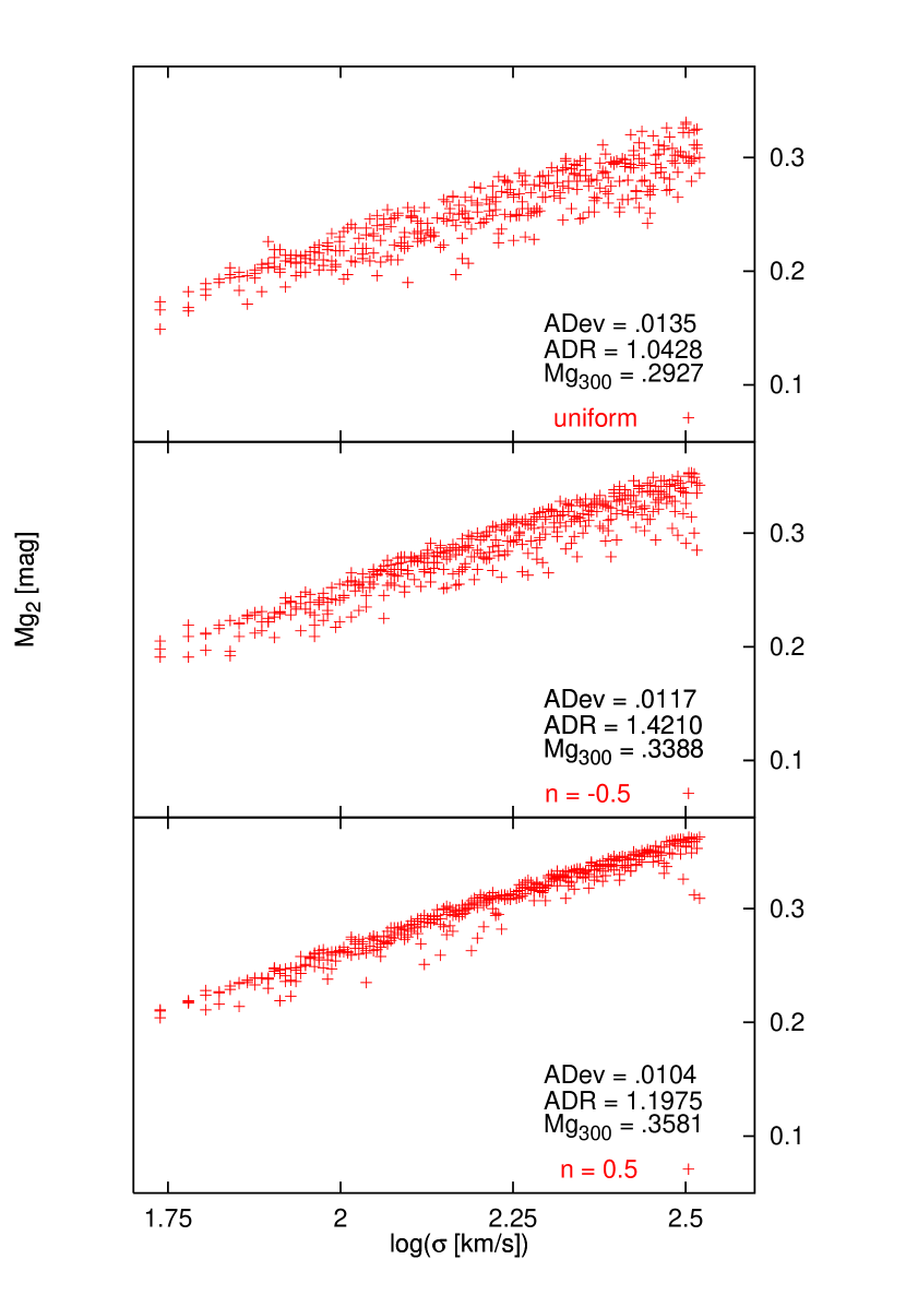
Figure 5: Influence of the number of equal-mass merger for 5, 40 and 80 mergers, with a uniform probability envelope, F${}_{gas}=0.2$, and a fraction of galaxy formed at z=z_f of F${}_{ini}=0$.

Figure 6: Influence of the probability for uniform probability, $n=-0.5$, and $n=0.5$, with 40 mergers, F${}_{gas}=0.2$, and F${}_{ini}=0$ .

As an introduction to the model output, we focus on examples of the effect of our four main parameters. Figure 6 shows the effect of varying the number of equal-mass mergers that eventually form the galaxy. With a lot of mergers (80 mergers, for example), the asymmetry becomes low since all the galaxies have almost the same history. That is, they all suffer a peppering of small amounts of star formation over the age of the universe. But with very few mergers (5 mergers, for example) the dispersion is larger and the asymmetry is much more pronounced. Each galaxy experiences a distinct timing fingerprint for mergers and thus are more individualistic, some having had recent star formation, others having had none.

The shape of the probability envelope has a strong impact as well. The frequency of mergers is often parameterized in the literature as being proportional to $(1+z)^{n}$, where $n$ is a free parameter. Figure 9 translates some of these choices from redshift to time. One can see that $n=-1.2$ roughly corresponds to a uniform probability with time (note that when we say “uniform probability” throughout this paper, we mean a perfectly flat [with time] curve, avoiding altogether the $(1+z)^{n}$ formalism.); $n=-0.7$ corresponds to a present-day merger frequency about half of that at $z=z_{f}$, and $n>0$ corresponds to merger rates strongly skewed to high redshift. These numbers change somewhat with cosmology.

As fig 6 shows, it is plain that with $n=0.5$ the obtained distribution is very thin. Since mergers are concentrated in the past, few are lucky enough to have had recent star formation. The relation thickens with decreasing $n$.

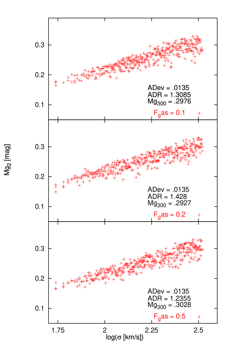
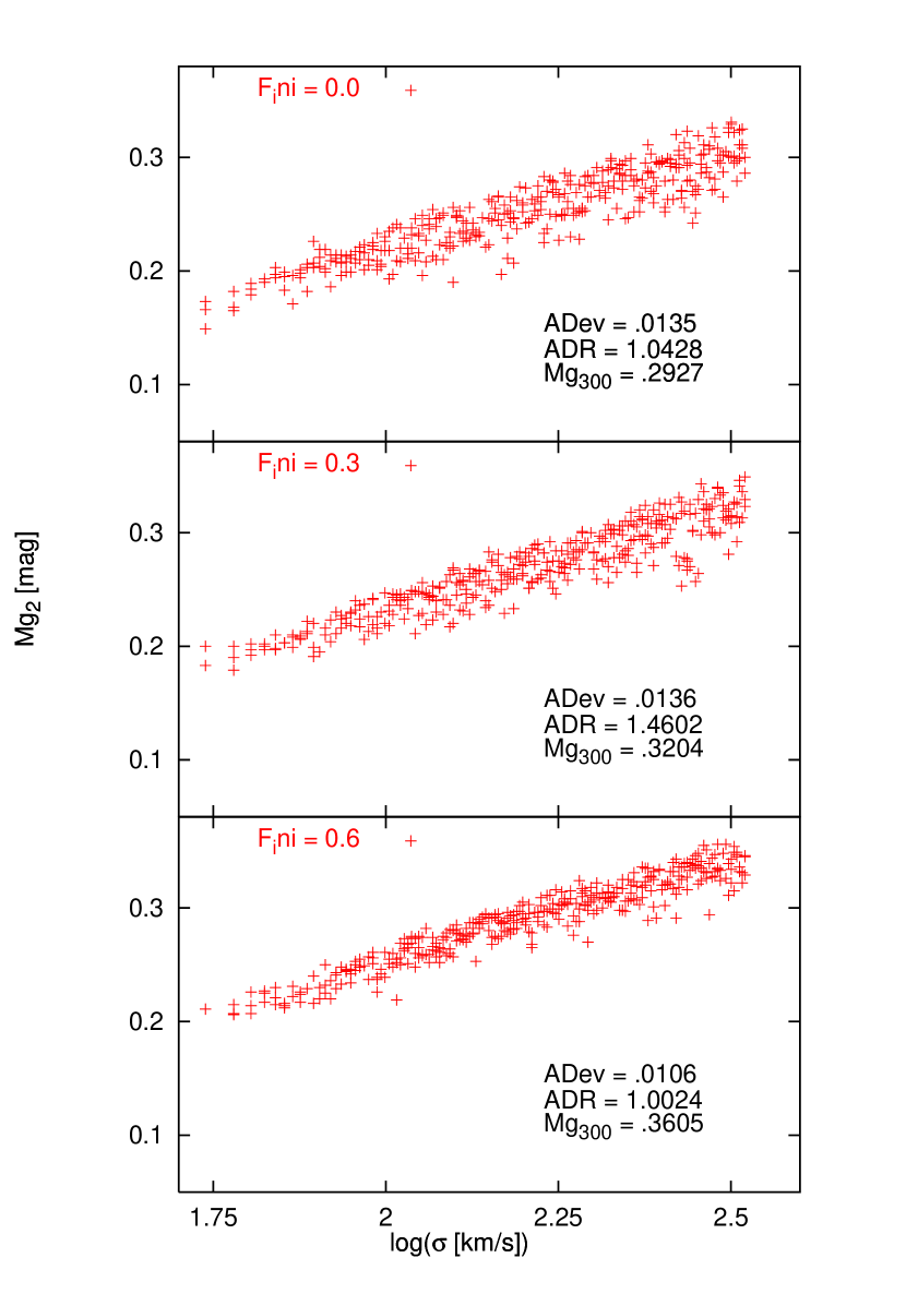
Figure 7: Influence of the fraction of gas in each merging event, for 3 different gas fractions, F${}_{gas}=$ : .1, .2 and .5, for 40 mergers, a uniform probability envelope, and a fraction of galaxy formed at z=z_f, F${}_{ini}=0$.

Figure 8: Influence of the fraction of the galaxy formed at z=z_f, for 3 different initial fractions, F${}_{ini}=$ 0, 0.3 and 0.6, for 40 mergers, a uniform probability envelope and F${}_{gas}=0.2$.

The parameter $F_{gas}$ is the fraction of gas used in each merger event. In Figure 8 we see that more gas leads to more star formation and hence more young galaxies. Less gas leads to weak starbursts and a narrow Mg-$\sigma$ relation.

The fraction of galaxy formed at $z=z_{f}$, $F_{ini}$, has less of a dramatic effect (see fig 8) except for the trivial case of $F_{ini}\approx 1$. There is little difference between forming half of the galaxy at $z_{f}$ and forming the galaxy entirely by mergers, rather to the initial surprise of the authors. Apparently, it is the last few Gyr of history that are the most important.

4.2 Maximum Merger Models

We now search quantitatively for solutions under the maximum merger hypothesis. For fair statistical comparison, the artificial data were further randomized by an artificial Gaussian scatter $\sigma_{a}=0.01$ mag, representing the observational error only. That is, $\sigma_{a}<\sigma_{g}$, the width of the Gaussian core of the residual distribution. This assumption is modified for the “ancient formation” hypothesis described below.

Because we compare to the mean of all of the observational data, we analysed data from a similar number of artificial galaxies: roughly 2000 Monte Carlo galaxies. The scatter from limited sample size of course decreases with increased number of samples: for 250 galaxies the errors were .0009 and .2 for respectively the ADev and the ADR (computed from multiple realizations of the same simulation). With 2000 galaxies we obtained .0002 for the ADev and .04 for the ADR. These errors are not too different from those seen in the observational data sets, so it is all but certain that sampling error causes most of the statistical deviations between data sets. This leads to important guidelines for future work at higher redshift: large sample size is crucial if the scatter is to be adequately characterized, and errors may not creep too much higher than their nearby brethren.

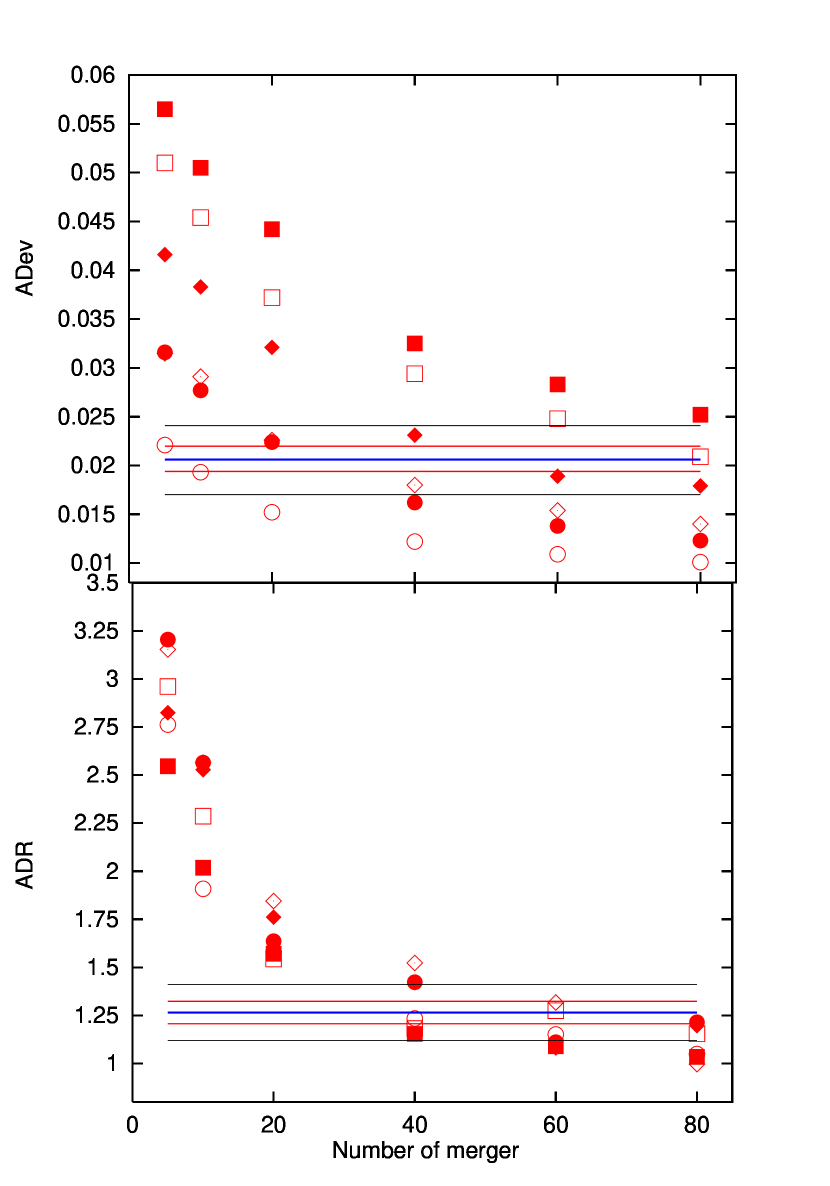
Figure 10: ADev (top) and ADR (bottom) for a uniform probability versus the number of mergers. For F${}_{ini}=0.0$, filled bullets, diamonds, and squares represent F${}_{gas}=.1,.2,.5$, respectively. For F${}_{ini}=0.5$, open bullets, diamonds, and squares correspond to F${}_{gas}=.1,.2,.5$, respectively. The central lines are the observational means with other lines situated at $\pm\sigma$ and $\pm 2.5\,\sigma$. An artificial observed scatter of $\sigma_{a}=0.01\,mag$ was included.

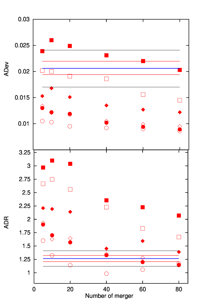
Figure 11: ADev (top) and ADR (bottom) for a (1+z)⁰ probability versus the number of mergers. An artificial observed scatter of $\sigma_{a}=0.01\,mag$ was included. Symbols and lines are the same as fig. 10.

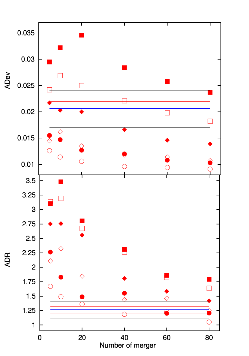
Figure 12: ADev (top) and ADR (bottom) for a (1+z)^-0.5 probability versus the number of mergers. An artificial observed scatter of $\sigma_{a}=0.01\,mag$ was included. Symbols and lines are the same as fig. 10.

Figures 10 through 12 show our main diagnostic statistics, ADev and ADR, for models that cover the grid of input parameters. Data for a uniform probability are shown in Figure 10, for a $(1+z)^{0}$ envelope in Figure 11, and for a $(1+z)^{-0.5}$ envelope in Figure 12. Different $F_{ini}$ and $F_{gas}$ possibilities are plotted as various symbol types as a function of the number of mergers. The trend with increasing number of mergers is clear: a tighter, more symmetrical relation is found. If this seems counterintuitive because with many mergers one should expect a more volatile and bursty collection of galaxies, consider instead that each galaxy has a more similar history if the number of mergers grows large. See also Figure 6. We plot a good sampling of the possibilities, representing F${}_{ini}=0.0$ or $0.5$ and F${}_{gas}=.1,.2,.5$ with different symbol types. To compare directly with the observational data, we plot the mean observational values found in $\S 2$ with $\pm 1.0\,\sigma$ and $\pm 2.5\,\sigma$ errors.

Other trends are also apparent. At a given F_ini, the ADev increases with the gas fraction since with more gas available more stars will form, making the mean stellar population more volatile. Similarly, at fixed gas fraction, the ADev decreases with higher $F_{ini}$. Indeed, if $F_{ini}$ is set to one, the relation becomes razor thin since the whole galaxy formed at $z=z_{f}$. Except for values approaching one, the authors were surprised at the ineffectiveness of $F_{ini}$ to modify the Mg-$\sigma$ relation by much; it is the weakest of the four parameters.

As for the influence of when in time the mergers are likely to happen, we compare the three figures. It is rather difficult to find many points that land simultaneously in the 2.5-$\sigma$ regions of both ADev and ADR statistics, but to the extent that some do, most of them are in the “uniform probability” figure, around 40 mergers. Any probability exponent $n$ greater than zero yields Mg-$\sigma$ relations that are even thinner than the $n=0$ case, and we are forced to conclude that elliptical galaxy formation that was concentrated to the first half of a Hubble time is ruled out under the maximum merger hypothesis.

4.3 Ancient Formation Models

We now relax our assumption that the Mg-$\sigma$ relation is inherently thin. We suppose instead that there is a intrinsic, symmetric scatter $\sigma_{g}$ equal to that which is observed today, but imprinted at formation. The mean width derived in $\S$2 is $\sigma_{g}=0.015$ mag. This is rather narrow and not too different from the observational scatter, 0.010 mag. In fact, consideration of these numbers implies that the true galaxy-intrinsic Gaussian-random scatter is around 0.01 mag. It will be interesting to see if future high-precision data upholds this conclusion.

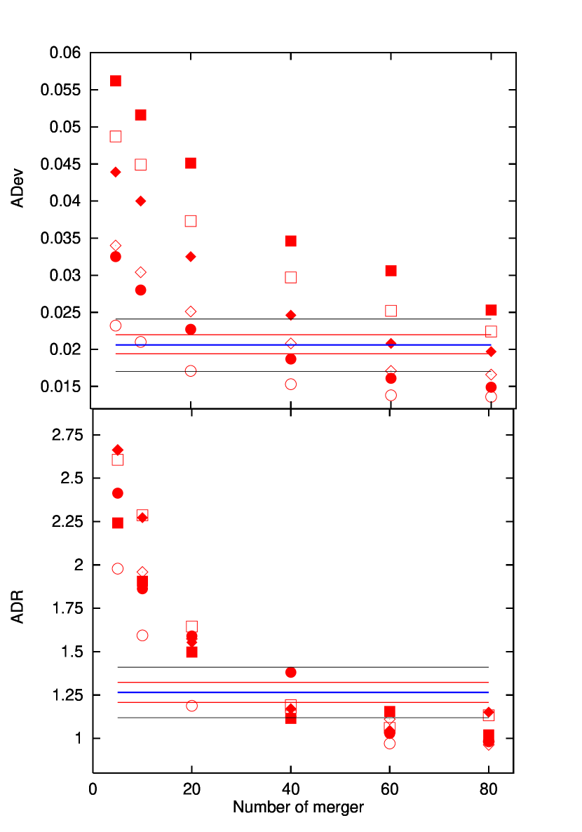
Figure 13: ADev (top) and ADR (bottom) for a uniform probability versus the number of mergers, with an artificial scatter $\sigma_{g}=0.015\,mag$. For F${}_{ini}=0.0$, filled bullets, diamonds, and squares represent F${}_{gas}=$ .1, .2, .5, respectively. For F${}_{ini}=0.5$, the open bullets, diamonds, squares correspond to F${}_{gas}=$ .1, .2, .5, respectively. The central lines are the observational means with other lines situated at $\pm\sigma$ and $\pm 2.5\,\sigma$ .

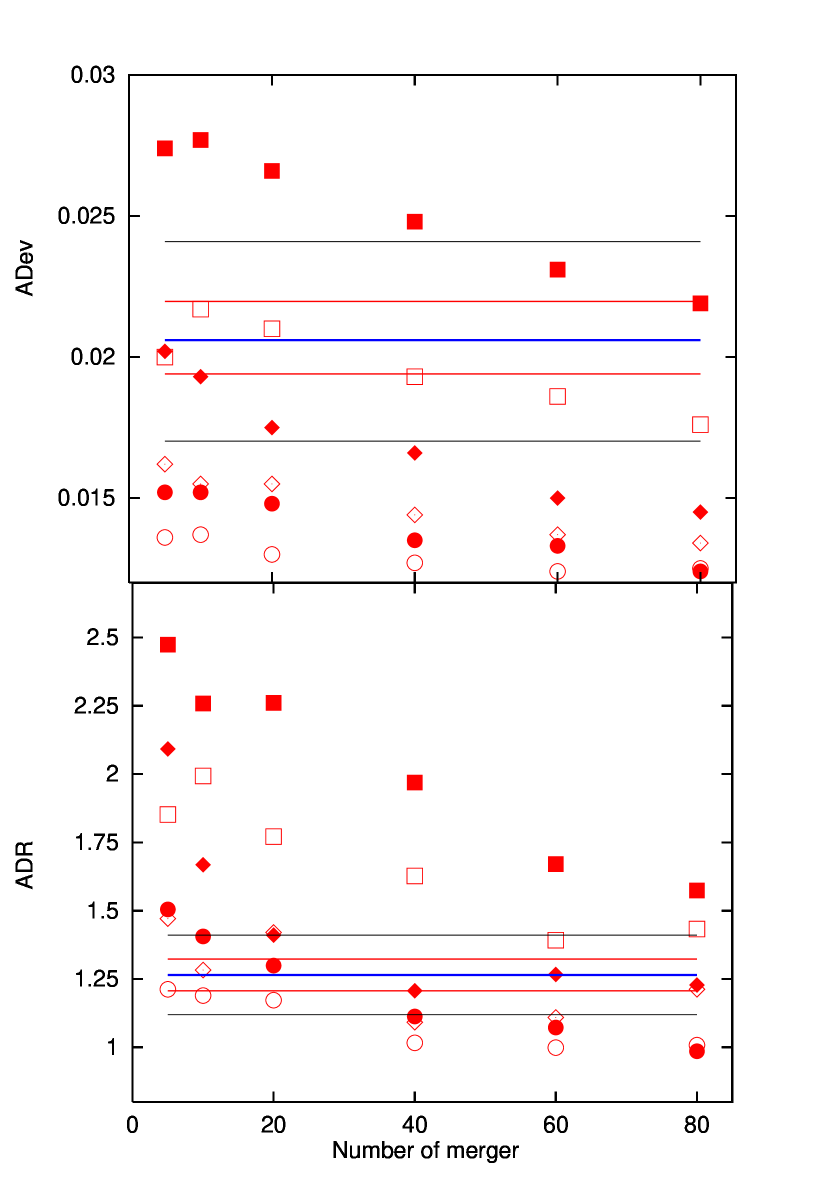
Figure 14: ADev (top) and ADR (bottom) for a (1+z)⁰ probability versus the number of mergers, with an artificial scatter $\sigma_{g}=0.015\,mag$. Symbols and lines are the same as fig. 13.

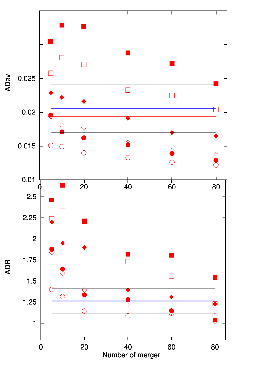
Figure 15: ADev (top) and ADR (bottom) for a (1+z)^-0.5 probability versus the number of mergers, with an artificial scatter $\sigma_{g}=0.015\,mag$. Symbols and lines are the same as fig. 13.

Under the ancient formation hypothesis, only the asymmetric tail of the distribution is produced by late star formation. Do these models fit better? We plot the three different probability cases exactly as in the previous section: uniform probability (fig 13), $(1+z)^{0}$ envelope (fig 14) and $(1+z)^{-0.5}$ envelope (fig 15). We derived the statistics using 2000 galaxies, and show the possibilities allowed by $F_{gas}=0.1,0.2,0.5$ and $F_{ini}=0.0$ or $0.5$.

We find that most of the remarks from last section are still valid. The cases with 5 or 10 mergers do not fit, and the most numerous solutions still occur for uniform probability and $N_{\rm merger}=40$. The main difference is that the additional artificial scatter calms the asymmetry somewhat, and this allows a few more successful models. We even find a couple of models in the $n=0$ panel that land within the error bars for both statistics, although mostly we find the width of the Mg-$\sigma$ relation too narrow.

The astounding similarity between maximum-merger and minimum-merger cases is driven by the high quality and consistency of the observational data. With the low and high bounds of allowed artificial scatter set at 0.010 and 0.015 mag, tight reigns are held on our freedom to interpret the results.

4.4 Constraints from Mg₃₀₀

To this point in the paper we have examined only ’primary’ statistics ADev and ADR for the width and asymmetry of the Mg-$\sigma$ residuals. We can explore the situation a little more by also considering the absolute Mg strength of the Mg-$\sigma$ relation, parameterized by Mg₃₀₀, the median Mg strength at $\sigma=$ 300 km/s. Including Mg₃₀₀ along with ADR and ADev, we define a goodness parameter to evaluate the relative merit of the various models:

$$\sigma^{2}_{G}=\frac{(ADev_{i}-\overline{ADev_{obs}})^{2}}{\sigma^{2}_{ADev}}+\frac{(ADR_{i}-\overline{ADR_{obs}})^{2}}{\sigma^{2}_{ADR}}+\frac{(Mg_{300_{i}}-\overline{Mg_{300_{obs}}})^{2}}{\sigma^{2}_{Mg_{300}}}$$

We took $\overline{ADev_{obs}}=.0206$ , $\overline{ADR_{obs}}=1.265$ and $\overline{Mg_{300_{obs}}}=0.329$, for the different scatters we had: $\sigma_{ADev}=1.4\,10^{-3}$, $\sigma_{ADR}=5.8\,10^{-2}$ and $\sigma_{Mg_{300}}=0.04$. This last value is less well-motivated than the others since we expect considerable uncertainty in model Mg zeropoint so that cannot adopt the observed uncertainty for $\sigma_{Mg_{300}}$. On the other hand, the overall Mg level is an important diagnostic and too-weak overall Mg is clearly to be discouraged, so our value of 0.04 is an approximate compromise.

We compute this $\sigma_{G}$ for the usual 3 cases : uniform merger probability envelope, (1+z)⁰ and (1+z)^-0.5 probability, and for both F${}_{ini}=0$ or $0.5$. For each case, we make plots from 5 to 100 mergers, and from F${}_{gas}=0$ to F${}_{gas}=0.9$, for 40 values using a linear distribution for the fraction of gas and a logarithmic distribution for the number of mergers. We plot isovalues in 1/$\sigma_{G}$ so that the best models show as maxima rather than minima. Fig 16 shows the results for uniform, (1+z)⁰ and (1+z)^-0.5 probability envelopes.

In this plot there are elongated regions of high $\sigma_{G}$ values. They tend to slant, indicating significant degeneracy between gas fraction and number of mergers in determining a successful model. The amplitude of the band decreases with the $n$ of the envelope probability. We see that the valid possibilities shift to slightly higher values of gas fraction when F${}_{ini}=0.5$. The uniform envelope probability appears to be the best fit.

4.5 Constraints from Mean Age and Abundance Spread

We now check to see if the possibly successful models indicated by ADev, ADR, and Mg₃₀₀ in Figure 16 are compatible with the abundance distribution and the V-band light-weighted age observed in nearby galaxies. The abundance distribution is observed to be narrow in all galaxies the size of M32 and larger (Worthey, Dorman & Jones, 1996), with a FWHM of less than 0.4 dex (Grillmair et al., 1996) in M32 itself, and about the same in the Milky Way (e.g. Rana (1991)). We can check the abundance distributions of the simulations as well. The chemical evolution of these models is primitive, but if the abundance distributions are wider than about 0.5 dex FWHM then we must regard them with suspicion. Also, if the light-weighted mean age (the closest our present models can come to approximating a spectroscopic Balmer-metal feature mean age) falls below about 7 Gyr (the approximate median of such studies, e.g. Terlevich & Forbes (2002); González (1993)) we likewise regard this model with much suspicion. Older ages are allowed because the age zeropoint of the Balmer-metal feature technique is still quite uncertain.

What we find is emphatic. For $n=0$ or $n=-0.5$ models, no model passes the ADR/ADev test very well, but they also tend to have an abundance scatter greater than 0.5 dex. For uniform probability, the mean galaxy age begins to becomes too young for a combination of high gas fraction and large numbers of mergers, but this never became a critical problem because the ADR/ADev test excludes these models as well. The best surviving model was with uniform probability, $F_{ini}=0.5$, $F_{gas}=0.35$, and 50 mergers, with an abundance histogram at the 0.5 dex width limit, mean age of 8.3 Gyr, and ADR and ADev within the error bars. At large number of mergers, the $F_{ini}=0.5$ models tend to have a bimodal abundance distribution caused by the initial metallicity of the galaxy, to which is added additional material from the gaseous portion of the merger, plus a low-metallicity peak from the stellar component of the relatively low-mass merger fragments. In fact, all of the $F_{ini}=0.5$ high points in Fig. 16 are at the borderline of having a too-wide abundance distribution, and we should penalize these models a couple of contour levels for this near-transgression. The $F_{ini}=0$ models do not suffer from this: they all have suitably narrow abundance distributions. We claim roughly equal success for both versions of the uniform-probability models, but resounding failure for models in which galaxy mergers happen preferentially in the past.

4.6 Model Variants

Being left with only one fully successful model after trying so many hundreds left the authors scratching their heads. We decided to explore other options. Our first option was to abandon the constant merger mass assumption by adopting a cold dark matter (CDM) power spectrum for galaxy merger fragments. We use the formulae from White & Frenk (1991) and Kauffmann & White (1992) which are based on Press & Schechter (1974) formalism. CDM clusters hierarchically with preferentially small masses in the early universe, building toward larger structures later on. We built a lookup table with 40 steps in redshift and 200 steps in mass in order to quickly invert the probability function for halos of a given mass and redshift. Within each step a small randomization assigned the final redshift and mass to the merger fragment. To calibrate the zero point between the circular velocity (V_c, which the White & Frenk formulae give) and mass, we normalized to the Milky Way. We took V${}_{c}=$ 220 km/s, mass equal to 10¹¹ M_⊙, and White & Frenk formulae to obtain M_gal= 10${}^{11}\,(\frac{V_{c}}{220\,km/s})^{3}$.

The only parameters in the CDM merger models were gas fraction and the CDM “bias” parameter $b$. The ADR statistics from the CDM models were very high unless the gas fraction was set below 10%, at which point the ADev becomes too narrow. The $V$-weighted age and abundance scatter for the $F_{gas}=0.1$ model is acceptable: 11.4 Gyr and 0.4 dex, respectively. Increasing the bias parameter helps a little, but no CDM models were found that matched all statistics simultaneously. The CDM simulations were also interesting because they predict variations in Mg-$\sigma$ as a function of galaxy size. For small galaxies compared to large, CDM predicts similar ADev, younger mean ages, and much higher asymmetry. Spectroscopic observations (Terlevich & Forbes, 2002) indicate a younger mean age for smaller galaxies. Our collection of Mg-$\sigma$ observations indicate higher ADev but ADR roughly the same.

A variant on the CDM models was to throw out the CDM power spectrum and adopt a constant power spectrum ($dN\propto M^{-1}$) and return to a merger probability uniform with time. These models have suitable ADR and ADev if the gas fraction is set at 2% - 3%. The 2% model has a ($V$-weighted) mean age of 11.7 Gyr, with an abundance distribution FWHM scatter of .3 dex. This is the only model with a mass spectrum (as opposed to the $F_{ini}$ plus constant $dM$ models) that fits all of the observational constraints. Consequently, even though this constant power spectrum model is not physical, the good fit seems to indicate that there will be some power spectrum that will satisfy the constraints equally well.

Other variants were tried. We tried superimposing two different schemes atop one another. For instance, suppose half of the galaxies were truly ancient and the other half was allowed to have mergers. These superposition schemes fail dramatically. Unless one is exquisitely artful one ends up with Mg-$\sigma$ diagrams that are clearly double.

Finally, we tried schemes of variable gas fraction, where the early universe was assumed to be gas rich, but later mergers are mostly stellar. Similarly to the regular 4-parameter models, envelope parameters $n>-0.5$ are ruled out, but uniform-with-time probability gives good matches for $20<N_{merger}<40$. In fact, one such model, with F_gas varying linearly with time from 0.9 at $z_{f}$ to 0.1 today matches the Mg-$\sigma$ data best of all models. This model is also intriguing because it shows strong Mg-$\sigma$ asymmetry evolution at only modest redshift (see next section).

4.7 Predictions for Lookback Studies

The recent proliferation of 8-12m telescopes will greatly accelerate the rate at which Mg-$\sigma$ data will become available for distant galaxies. The result of studies to date, that the drift of the Mg zero point is “consistent with passive evolution,” (Ziegler & Bender, 1997) will eventually be broadened to study the shape of Mg residuals as well. We therefore present some model predictions for high-redshift studies. There is a major caveat to consider here: model galaxies are assumed to be “star forming” for 50 Myr after a burst, but “early type” at all other times. If merging is a dominant process, then premerger fragments are often likely to be spiral galaxies. If semianalytic models like Kauffmann & White (1992) are correct, then, over time, some ellipticals can accrete a gas disk and become spirals. So the predictions we show in this section are of questionable validity for merger-dominated models (i.e. all of those that match the $z=0$ data!), but nevertheless provide a useful first cut for the variety of behavior we might expect for Mg-$\sigma$ relations at significant lookback times.

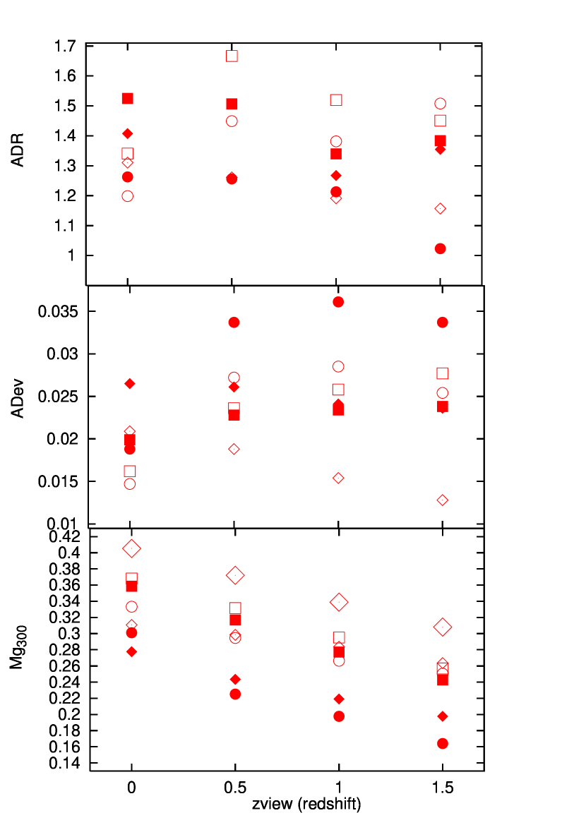
Figure 17: Evolution in the past for the ADR (top), ADev (middle) and the value of Mg₂ at 300 km/s (bottom). Zview is the lookback time given in redshift. The open squares are for a constant power spectrum model with F${}_{gas}\,=2$ % and the filled squares plot the CDM model with F${}_{gas}=0.1$. The bullets represent the variable gas fraction model with 30 mergers and a uniform probability (filled for F${}_{ini}=$ 0, open for F${}_{ini}=$ 0.5). The diamonds plot the regular model with a uniform probability, 40 mergers and F${}_{gas}\,=\,0.25$ (filled for F${}_{ini}=$ 0, open for F${}_{ini}=$ 0.5) . The bigger open diamonds represent the evolution for F${}_{ini}=$ 1.

Figure 17 shows a collection of near-best models as they would appear if observed at large lookback times. The merging trees of the model galaxies are computed to redshift zero, but only the partially complete history of each galaxy is considered for nonzero redshift. So the further back in time we look, the more incomplete the galaxies are. Figure 17 at a glance shows that Mg-$\sigma$ relations survive intact even under fairly severe merging scenarios back to when the Universe was a quarter of its present age.

The bottom panel shows Mg₃₀₀ as a function of redshift. Within a zeropoint shift, all models show Mg evolution very similar to the “ancient, passive evolution” case shown in large diamond symbols at strong Mg strength. It is easy to shift any given model track by adjusting the assumed metallicity scale, so the overall Mg level by itself is not a strong constraint, but the relative time evolution should be fairly well modeled. The most shallow slope, that is, the most constant Mg level with time, is given by the $F_{gas}=0.25$, 40-merger, uniform probability, $F_{ini}=0.5$ model (small open diamonds). This is a merger-heavy model. We think that some researchers will be surprised by the fact that a merger-driven model is redder, relatively speaking, at $z=1.5$, than pure passive evolution scenario because one usually thinks of mergers as causing more star formation activity and hence bluer colors and weaker line strengths. In reality, it can go either way depending on the model. The steepest Mg track is from a very similar model but with the variable $F_{gas}$ option and $F_{ini}=0$ (filled bullets). Neither steepest nor shallowest models differ by more than 0.05 mag in Mg₃₀₀ from the passive evolution case if they are normalized to match at one end or the other of the illustrated redshift range.

The tightness and asymmetry of the Mg-$\sigma$ relation also do not show large changes with lookback time. Both the ADR and ADev can increase or decrease according to the model, but at a very modest level that will be hard to measure without a very large sample of distant galaxies.

5 Summary and Synthesis

In this paper we analyze the Mg-$\sigma$ relation in elliptical and S0 galaxies by comparing data and models.

We adapted an “ADR” statistic for the measuring residual asymmetry and we used the ADev statistic to measure the width of the scatter. For the combination of all data sets and for 150 $<\sigma<$ 320 km s^-1, ADev $=$ .0206 $\pm$ .0014, ADR $=$ 1.265 $\pm$ 0.058 and Mg${}_{300}=$ 0.329 $\pm$ .0039 . The width of the distribution increases at low $\sigma$. For 50 $<\,\sigma\,<$ 150 km s^-1 the ADev $=$ .0282 $\pm$ .0035. The errors of the ADev and ADR statistics are roughly consistent with the random errors one would expect from finite number counting as estimated from running simulations multiple times (the observed ADR scatter is even somewhat lower that what we would expect).

We also fit the central peak of the Mg residual distribution with a Gaussian, thinking that this would be a useful number to know under an ancient formation hypothesis where all of this scatter was imprinted at formation. We found a width for the central peak of the Mg residual $\sigma_{g}=$ .014 $\pm$ .002 mag, for Mg₂ while the observational error was $\sigma_{obs}=0.010$. So if total scatter is a quadrature sum of observational and intrinsic scatter, that is, $\sigma^{2}_{g}=\sigma^{2}_{intrinsic}\,+\,\sigma^{2}_{obs}$, we find $\sigma_{intrinsic}=.01\,mag$. After performing this exercise we realized that there would be little difference for models that began with the entire scatter or just the observational portion of the scatter, and this turned out to be true: the “ancient formation” models were not dramatically different from the “maximum merger” models.

Merger models were constructed to simulate the Mg-$\sigma$ relation. The merger fragments that join to form the final galaxy were assumed to be equal in mass. Mergers occur randomly in time (uniform probability distribution) or randomly under a probability envelope of the form $(1+z)^{n}$, where $n$ is a free parameter. The other three main parameters are the number of mergers, the gas fraction of each event, and the fraction of the galaxy that formed in the distant past, at $z=z_{f}=5$ for this paper. Also included was an artificial scatter in Mg strength. This scatter was set equal to the observational error for the “maximum merger” hypothesis, and equal to the entire symmetric scatter for the “ancient formation” hypothesis, but since the latter was only 40% larger than the former, the two hypotheses generated similar results.

The models predict a simulated Mg-$\sigma$ diagram, from which we compute Mg₃₀₀, ADev, and ADR in the same way as we did for the observational data. We also output V-weighted mean age and an abundance distribution since observational constraints also exist on these quantities. Some immediate conclusions are:

$\bullet$ A small number (5-20) of (severe) mergers leads to scatter and asymmetry larger than observed.

$\bullet$ To the contrary, with many mergers (60-100) a large number of small events leads to small scatter and small asymmetry because merging histories are similar. Most of these models showed too tight of a relation, and the gas-rich ones also tended toward unacceptably young mean ages.

$\bullet$ For the merger probability envelope, a positive $n$ in $(1+z)^{n}$ concentrates galaxy formation to the early universe, making the Mg-$\sigma$ relation thin. Because we find no successful models for $n>0$, we clash with many published merger rate results such as $(1+z)^{2.3\pm 0.2}$, $(1+z)^{2.3\pm 0.9}$, $(1+z)^{4.5}$, or $(1+z)^{3.1{\rm\ or\ }2.5}$ (Conselice et al., 2001; Patton et al., 2002; Okamoto & Habe, 2000; Governato et al., 1999) but we agree with a few such as $(1+z)^{0.1\pm 0.5}$ (Carlberg et al., 2000). Our $n<0$ result is very robust, so we presume that the difference between this result and others stems from differences in treatment (i.e. redshift range, galaxy types, definition of merger rate, observables). For example, Kauffmann, Charlot, & White (1996) find a $(1+z)^{1.5}$ dependence for early type galaxies, but this is for number evolution, a quantity that we do not model because it requires tranformations to other Hubble types.

$\bullet$ An increased gas fraction increases the number of new stars formed in each merger. This increases the scatter in Mg strength but increases asymmetry only on some models.

$\bullet$ If a larger fraction of the galaxies form at $z=z_{f}$, both scatter and asymmetry decrease.

Finally, let us briefly discuss the meaning of these results. Our most successful models involved a moderate number of mergers (20-60) with mergers equally probable over cosmic time. The model with a constant gas fraction that fit the best was with $F_{gas}=0.15$-0.3 but a model with gas fraction that varies linearly with time from 0.9 at $z_{f}$ to 0.1 at the present epoch fit even better. One other model, a variable-mass scenario with a flat power spectrum and merger probability constant with time fit the constraints if the gas fraction was 2% - 3%. The overall yield of successful models was far below our initial expectations; we thought many solutions would be possible. This is good news for understanding galaxy evolution: tight constraints are better than loose ones.

We also find some clarity for the basic question, “Are ellipticals old or young?” To arrive at age information, one must look at the most sensitive indicators. A brief perusal of Worthey (1994) or other population model paper weighted by the inverse of the observational error orders the list, from most sensitive to least sensitive: Balmer-metal diagrams, Mg-$\sigma$ relation, Fundamental Plane, and color-magnitude diagram. Thus Balmer-metal diagrams show very large age scatter that is harder to detect with other methods. The present study of the Mg-$\sigma$ relation finds that the models that fit every observable have an age range of 7-10 Gyr. This does not force a revision of the Balmer-based age scale, but it keeps alive the long-held suspicion that the Balmer ages are all somewhat too young. The Balmer-derived age scatter is fully supported by our study.

(1) Balmer-metal and Mg-$\sigma$ diagrams are compatible, both implying considerable age scatter and a mean age (7-10 Gyr) within the uncertainty of the Balmer method. The tightness of the Mg-$\sigma$ relation is compatible with the less-sensitive FP and color-magnitude diagram tightness, and both are compatible with the Balmer-metal diagrams. In short, we see no barriers to fairly strong merger hypotheses.

(2) In contrast, we find little support for the ancient merger hypothesis: the tamest merger scenarios that we could find are still much wilder than quiescent evolution since $z_{f}$. The least active model (2-3% gas fraction and flat mass spectrum) still involves massive mergers (albeit without much gas) up to the present time. On the other hand, this model’s mean age was 11 Gyr and it was still able to match the width and asymmetry of the Mg-$\sigma$ relation, so there may be a related model that can satisfy a relaxed version of the ancient merger hypothesis.

We found this avenue of investigation unexpectedly fruitful in the sense that very strong observational constraints allow only very select interpretations to survive. Future theoretical work should involve more choices for mass power spectrum as a first priority, although many aspects of the modeling could be improved. Observational work at intermediate redshift is also needed, although our results regarding high quality and large $N$ of such studies make this job more challenging.

Table 1: Statistics on the Different Data Sets

Paper	N	N${}^{{}^{\prime}}$	Mg 300	Std. Dev.	Skewness	ADev	ADR	$\sigma_{g}$
Mg2
Prugniel, Simien 1996	644	246	0.314	0.023	-1.017	0.017	1.120	0.013
Trager et al. 1998 (Lick)	256	183	0.339	0.032	-1.750	0.022	1.544	0.014
Efar 1999	140	130	0.331	0.021	-0.324	0.017	1.210	0.013
Dressler et al. 1991	123	107	0.318	0.023	-0.722	0.018	1.538	0.011
Bernardi et al. 1998 (all)	721	654	0.329	0.033	-0.184	0.025	1.230	0.020
Bernardi et al. 1998 (field)	469	366	0.331	0.033	-0.186	0.025	1.151	0.020
Bernardi et al. 1998 (group)	104	91	0.333	0.031	-0.369	0.024	1.361	0.015
Bernardi et al. 1998 (cluster)	104	83	0.331	0.032	-0.052	0.023	1.128	0.013
Hudson 2001	528	391	0.332	0.018	-0.369	0.014	1.105	0.013
Mg$b$
Trager et al. 1998 (Lick)	256	183	5.091	0.526	-0.971	0.378	1.220	0.2
Efar 1999	164	144	5.260	0.422	-0.573	0.314	0.990	0.3
$<$Mg2$>$
Trager et al. 1998 (Lick)	256	183	0.338	0.032	-2.472	0.021	1.788	0.011
7-Samurai	577	358	0.324	0.038	-5.545	0.020	1.609	0.015

Note. — Col. (1)—Reference. Col. (2)—Number of galaxies in the sample. Col. (3)—Number of galaxies used for the statistic. Col. (4)—Value of the Mg index at $\sigma=300\,km/s$. Col. (5)—Standard deviation. Col. (6)—Skewness. Col. (7)—ADev or Average Deviation. Col. (8)—ADR or Average Deviation Ratio. Col. (9)— $\sigma$ from the (Gaussian) fit.

Figure 9: Merger probability as a function of time. For higher $(1+z)^{n}$ exponents, merging events happen preferentially early. The “uniform” probability often used in this article would be represented by a horizontal line in this diagram.

Figure 16: Isovalue contours of $\frac{1}{\sigma_{G}}$ for a uniform probability (top), $n=0$ probability (middle), and $n=-0.5$ probability (bottom) for F${}_{ini}=0$ (left) and $0.5$ (right). An artificial observed scatter of $\sigma_{a}=0.01\,mag$ was included. The contours are set at multiples of $\sqrt{3}/4$ so that borderline acceptability corresponds approximately to the second contour level, “good” fits to the fourth.

References

- Bardelli et al. (2002) Bardelli, S., De Grandi, S., Ettori, S., Molendi, S., Zucca, E. & Colafrancesco, S. 2002, A&A, 382, 17
- Bender et al. (1992) Bender, R., Burstein, D. & Faber, S. M. 1992, ApJ, 399, 462
- Bender et al. (1993) Bender, R., Burstein, D. & Faber, S. M. 1993, ApJ, 411, 153
- Bender et al. (1998) Bender, R., Saglia, R. P., Ziegler, B., Belloni, P., Greggio, L. & Hopp, U. 1998, ApJ, 493, 529
- Bernardi et al (1998) Bernardi, M., Renzini, A., Da Costa, L.N.,Wegner, G., Alonso, V., Pellegrini, P. S., Rité, C. & Willmer, C.N.A. 1998, ApJ, 508, 143
- Bertelli et al. (1994) Bertelli, G., Bressan, A., Chiosi, C., Fagotto, F. & Nasi, E. 1994, A&A, 106, 27
- Burstein et al. (1990) Burstein, D., Faber, S. M. & Dressler, A. 1990, ApJ, 354, 18
- Carlberg et al. (2000) Carlberg, R. G., Cohen, J. G., Patton, D. R., Blandford, R., Hogg, D. W., Yee, H. K. C., Morris, S. L., Lin, H., Hall, P. B., Sawicki, M., Wirth, G. D., Cowie, L. L., Hu, E., Songaila, A. 2000, ApJ, 532, L1
- Colless et al. (1999) Colless, M., Burstein, D., Davies, R. L., McMahan, R. K., Saglia, R. P., & Wegner, G. 1999, MNRAS, 303, 813
- Conselice et al. (2001) Conselice, C. J., Bershady, M. A. & Dickinson, M. 2001, BAAS, 198, 3417
- Davies et al (1987) Davies, R. L., Burstein, D., Dressler, A., Faber, S. M., Lynden-Bell, D., Terlevich, R. J. & Wegner, G. 1987, ApJS, 64, 581
- Djorgovsky & Davies (1987) Djorgovsky, S. & Davies, M. 1987, ApJ, 313, 59
- Dressler et al. (1987) Dressler, A., Lynden-Bell, D., Burstein, D., Davies, R. L., Faber, S.M., Terlevitch, R. J. & Wegner, G. 1987, ApJ, 313, 42
- Dressler et al. (1991) Dressler, A., Faber, S. M. & Burstein D. 1991, ApJ, 368, 54
- Ellis et al. (1997) Ellis, R. S., Smail, I., Dressler, A., Couch, W. C., Oemler, A., Butcher, H. & Sharples, R. M. 1997, ApJ, 483, 582
- Forbes et al. (1998) Forbes, D. A., Ponman, T. & Brown, R. 1998, ApJ, 508, L43
- Forbes et al. (2001) Forbes, D. A., Beasley, M. A., Brodie, J. P. & Kissler-Patig, M. 2001, ApJ, 563, 143
- González (1993) González, J. J. 1993, Ph. D. Thesis, University of California, Santa Cruz
- Goudfrooij et al. (2001) Goudfrooij, P., Mack, J., Kissler-Patig, M., Meylan, G. & Minniti, D. 2001, MNRAS, 322, 643
- Governato et al. (1999) Governato, F., Gardner, J. P., Stadel, J., Quinn, T., & Lake, G. 1999, AJ, 117, 1651
- Grillmair et al. (1996) Grillmair, C. J., Lauer, T. R., Worthey, G., Faber, S. M., Freedman, W. L., Madore, B. F., Ajhar, E. A., Baum, W. A., Holtzman, J. A., Lynds, C. R., O’Neil, E. J., Jr., Stetson, P. B. 1996, AJ, 112, 1975
- Hudson et al. (2001) Hudson M. J., Lucey J. R., Smith R. J., Schlegel D. J. & Davies R. L. 2001, MNRAS, 327, 265
- Jørgensen et al. (1996) Jørgensen, I., Franx, M. & Kjœgaard, P. 1996, MNRAS, 280, 167
- Kauffmann, Charlot, & White (1996) Kauffmann, G., Charlot, S., & White, S. D. M. 1996, MNRAS, 283, 117
- Kauffmann & White (1992) Kauffmann, G. & White, S. D. M. 1993, MNRAS, 261, 921
- Kelson et al. (1997) Kelson, D. D., van Dokkum, P. G., Franx, M., Illingworth, G.D. & Fabricant, D. 1997, ApJ, 478, L13
- Kodama & Arimoto (1997) Kodama, T. & Arimoto, N. 1997, A&A, 320, 41
- Kodama et al. (1998) Kodama, T., Arimoto, N., Barger, A. J. & Aragón-Salamanca, A. 1998, A&A, 334, 99
- Larson (1975) Larson, R. B. 1975, MNRAS, 173, 671
- Markevitch et al. (2002) Markevitch, M., Gonzalez, A. H., David, L., Vikhlinin, A., Murray, S., Forman, W., Jones, C. & Tucker, W. 2002, ApJ, 567, 27
- Okamoto & Habe (2000) Okamoto, T., & Habe, A. 2000, PASJ, 52, 670
- Patton et al. (2002) Patton, D. R., Pritchet, C. J., Carlberg, R. G., Marzke, R. O., Yee, H. K. C., Hall, P. B., Lin, H., Morris, S. L., Sawicki, M., Shepherd, C. W., & Wirth, G. D. 2002, ApJ, 565, 208
- Press & Schechter (1974) Press, W. H. & Schechter, P. L. 1974, ApJ, 187, 425
- Prugniel & Simien (1996) Prugniel, P. & Simien, F. 1996, BAAS, 309, 749
- Rana (1991) Rana, N. C. 1991, ARA&A, 29, 129
- Schweizer et al. (1990) Schweizer, F., Seitzer, P., Faber, S. M., Burstein, D., Dalle Ore, C. M. & González, J. J. 1990, ApJ, 364, L33
- Schweizer & Seitzer (1992) Schweizer, F. & Seitzer, P. 1992, AJ, 104,1039
- Stanford et al. (1998) Stanford, S., Eisenhardt, P. & Dickinson, M. 1998, ApJ, 492, 461
- Terlevich & Forbes (2002) Terlevich, A. I. & Forbes, D. A. 2002, MNRAS, 330, 547
- Toomre (1977) Toomre, A. 1977, in The Evolution of Galaxies and Stellar Populations, ed. B. M. Tinsley & R. B. Larson (Yale Univ. Observatory: New Haven), 401
- Trager et al. (1998) Trager, S. C., Worthey, G., Faber, S. M., Burstein, D. & González, J. J. 1998, ApJS, 116, 1
- van Dokkum & Franx (1996) van Dokkum, P. G. & Franx, M. 1996, MNRAS, 281, 985
- van Dokkum et al. (1998) van Dokkum, P. G., Franx, M., Kelson, D. D. & Illingworth, G. D. 1998, ApJ, 504, 17
- Wegner et al. (1999) Wegner, G., Colless, M., Saglia, R. P., McMahan, R. K. Jr, Davies, R. L., Burstein, D. & Baggley, G. 1999, MNRAS, 305, 259
- White & Frenk (1991) White, S. D. M. & Frenk, C. S. 1991, ApJ, 379, 52
- Worthey (1994) Worthey, G. 1994, ApJS, 95, 107
- Worthey et al. (1994) Worthey, G., Faber, S. M., González, J. J. & Burstein, D. 1994, ApJS, 94, 687
- Worthey, Trager, & Faber (1995) Worthey, G., Trager, S. C., & Faber, S. M. 1995, in Fresh Views of Elliptical Galaxies, ed. A. Buzzoni, A. Renzini, & A. Serrano, ASP Conference Series, 86, 203
- Worthey, Dorman & Jones (1996) Worthey, G., Dorman, B. & Jones, L. A. 1996, AJ, 112, 948
- Worthey (1997) Worthey, G. 1997, in Star Formation Near and Far, ed. S. S. Holt & L. G. Mundy, (AIP Press: Woodbury, NY), 525
- Ziegler & Bender (1997) Ziegler, B. L. & Bender, R. 1997, MNRAS, 291, 527