Constraints on Models for TeV Gamma Rays from Gamma-Ray Bursts
Abstract
We explore several models which might be proposed to explain recent possible detections of high-energy (TeV) gamma rays in association with low-energy gamma-ray bursts (GRBs). Likely values (and/or upper limits) for the source energies in low- and high-energy gamma rays and hadrons are deduced for the burst sources associated with possible TeV gamma-ray detections by the Project GRAND array. Possible spectra for energetic gammas are deduced for three models: 1) inverse-Compton scattering of ambient photons from relativistic electrons; 2) proton-synchrotron emission; and 3) inelastic scattering of relativistic protons from ambient photons creating high-energy neutral pions, which decay into high-energy photons. These models rely on some basic assumptions about the GRB properties, e.g. that: the low- and high-energy gamma rays are produced at the same location; the time variability of the high-energy component can be estimated from the FWHM of the highest peak in the low-energy gamma ray light curve; and the variability-luminosity relation of Fenimore & Ramirez-Ruiz (2000) gives a reliable estimate of the redshifts of these bursts. We also explore the impact of each of these assumptions upon our models. We conclude that the energetic requirements are difficult to satisfy for any of these models unless, perhaps, either the photon beaming angle is much narrower for the high-energy component than for the low-energy GRB or the bursts occur at very low redshifts (). Nevertheless, we find that the energetic requirements are most easily satisfied if TeV gamma rays are produced predominantly by inverse-Compton scattering with a magnetic field strength well below equipartition or by proton-synchrotron emission with a magnetic field strength near equipartition.
pacs:
98.70.Rz, 98.70.Sa, 95.55.VjI Introduction
Evidence has been accumulating for the arrival of GeV-TeV gamma rays in coincidence with low-energy ( MeV) gamma-ray bursts (GRBs). For example, EGRET detected seven GRBs which emitted high energy photons in the MeV to 18 GeV range (Schneid et al., 1992; Hurley, 1994; Catelli, Dingus, & Schneid, 1997). There have also been results suggestive of gamma rays beyond the GeV range (Amenomori et al., 1996; Padilla et al., 1998), although these were not claimed as firm detections. Evidence has also been reported for TeV emission in one burst out of 54 BATSE GRBs in the field of view of the Milagrito detector (Atkins et al., 2000). In another paper Poirier et al. (2003) reported suggestive evidence for sub-TeV gamma rays arriving in coincidence with GRBs which occurred near zenith above the Gamma Ray Astrophysics at Notre Dame (GRAND) air shower array. In that experiment, most of the eight bursts analyzed were associated with at least some marginal excess () of muons including the event detected by Milagrito. One burst evidenced a possible detection at the level. As shown in Poirier et al. (2003), if this detection is real, then the output in energetic gammas is likely to dominate the energetics of the burst.
Although these data are not overwhelmingly convincing, they are at least suggestive that detectable energetic TeV gamma rays might be associated with low-energy gamma-ray bursts (Vernetto, 2000). Moreover, these new detections, if real, can not be explained by a simple extrapolation of the BATSE spectrum (Poirier et al., 2003), particularly if intergalactic absorption is taken into account (Salamon & Stecker, 1998; Totani, 2000). A new TeV component in the GRB spectrum seems to be required.
The present work is therefore an attempt to interpret these new possible detections in the context of three models, which might be proposed for the production of TeV gammas in a GRB. These are: 1) inverse-Compton scattering of ambient photons from relativistic electrons in the burst environment; 2) proton-synchrotron emission (Vietri, 1997; Totani, 1998a, b, 2000); and 3) inelastic scattering of relativistic protons from ambient photons creating high-energy neutral pions, which decay into high-energy photons (Waxman, 1995; Waxman & Bahcall, 1997). We here briefly outline the underlying physics and characteristic energetic gamma-ray spectra associated with each of these possible models. We then derive limits on the parameters of these models based upon the detection limits from the Project GRAND array. Based upon this, we conclude that it is difficult for any of these models to satisfy the energetic requirements unless the photon beaming angle is very narrow for the high-energy component. Of the models considered, the most likely are inverse-Compton scattering or proton-synchrotron emission. We note, however, that these conclusions rely upon a few assumptions. For example, we have assumed that the low- and high-energy gamma rays are produced at the same location; that the time variability of the high-energy component can be estimated from the FWHM of the highest peak in the low-energy gamma ray light curve; and that the variability-luminosity relation of Fenimore & Ramirez-Ruiz (2000) gives a reliable estimate of the redshifts of these bursts. We explore the impact of each of these assumptions and find that, unless the bursts occur at very low redshifts (), the energetic requirements remain difficult to satisfy.
II Low-Energy GRB Properties
The mystery of the astrophysical origin for low-energy gamma ray bursts (GRBs) has been with us for some time. As of yet there is no consensus explanation, although there is mounting evidence for an association with supernovae (Garnavich et al., 2002). A likely scenario is a burst environment involving collisions of an ultra relativistic plasma fireball (Paczyński, 1986; Goodman, 1986; Sari, Piran, & Narayan, 1998). These fireballs may produce low-energy gamma rays either by “internal” collisions of multiple shocks (Paczyński & Xu, 1994; Mészáros & Rees, 1994), or by “external” collisions of a single shock with ambient interstellar material (Rees & Mészáros, 1992).
In either of these paradigms it is possible for very energetic gammas to be produced through inverse-Compton scattering of ambient photons off the relativistic electrons. Furthermore, it seems likely that baryons would be accelerated along with the pair plasma to very high energies (Vietri, 1995; Waxman, 1995; Totani, 1998a). Synchrotron emission from energetic protons (Vietri, 1997; Böttcher & Dermer, 1998; Totani, 1998a, b) or possibly hadro-production of pions in the burst environment (Waxman & Bahcall, 1997) and subsequent gamma decay could also lead to an additional spectral component of very energetic gammas. In any case, it is at least plausible that energetic gammas could arrive in coincidence with a gamma-ray burst. This was the premise of Project GRAND’s search for high-energy gammas arriving in coincidence with BATSE GRB observations.
It is also possible, however, that low- and high-energy gamma-ray components are generated in different regions or phases of a burst. This could lead to substantially different arrival times for each component. This was in fact the case for the 18 GeV photon observed by EGRET, which arrived s after the low-energy emission had ended.
Observations of TeV gammas could provide important clues as to the baryon loading, Lorentz factor, and ambient magnetic field of the relativistic fireball. Our goal in this paper is to constrain the possible spectrum and source of energetic photons using the Project GRAND data. Hence, we restrict ourselves to considering high-energy gammas produced concurrently with low-energy gammas consistent with the search technique employed by Project GRAND.
III Fits to Observed GRB Spectra
Table 1 summarizes some of the features of the BATSE and Project GRAND observations of the eight GRBs analyzed in Poirier et al. (2003), where a detailed explanation of the Project GRAND results can be found. In the present paper, we will denote quantities in the frame of the observer by the superscript “”. We will also use to denote the low energy GRB photons and distinguish them from the high-energy component, denoted . The observed BATSE spectra are fit with a broken power law of the form (Band et al., 1993)
| (1) |
where , , and MeV is the break energy of the observed spectrum. Although these bursts are often better fit by using an exponential to join the two components, a broken power law is adequate for the present discussion. It maintains a simple analytic form for the equations, and as we shall see, the precise low energy form is almost irrelevant as long as a break energy exists. In what follows we will use values of , , , and derived from optimum fits to the BATSE spectra for all events except the Milagrito event for which the BATSE fluence was too weak to obtain a reliable spectral fit. The BATSE fit parameters corresponding to equation (1) are listed in Table 2. The fit parameters for these bursts were provided at our request by M. S. Briggs at the Marshall Space Flight Center. We also include the variability time scale for these bursts, which was estimated as the full width at half maximum (FWHM) of the brightest peak in each light curve. The light curves of GRBs typically show a wide range of timescale variability, so this choice may not be justified. In §VII we explore the dependence of our conclusions on a wide range of values for .
In Table 3, we give estimated redshifts for each burst. GRB 990123 is the only burst in this group for which an optical counterpart was detected. This burst, therefore, is known to have occurred at a redshift of (Kulkarni et al., 1999). The redshifts for most of the remaining bursts were estimated using the variability-luminosity relation of Fenimore & Ramirez-Ruiz (2000). This method relies on the apparent correlation between the time variability of a burst, which can be measured from its light curve, and the absolute luminosity of the burst, which we wish to infer. This provides us with a straightforward method for converting GRB observables into luminosities and redshifts (Fenimore & Ramirez-Ruiz, 2000).
Following Fenimore & Ramirez-Ruiz (2000), we first fit a quadratic polynomial to the background in the non-burst portions of the BATSE 64 ms four channel data (i.e. DISSC data). Let be the binned background counts from this polynomial fit. If are the observed binned counts during the actual burst event, then the net count is . We then rebin the counts by dilating the time samples by , where is the redshift we wish to estimate and is a baseline redshift. Following (Fenimore & Ramirez-Ruiz, 2000), we take . The new, dilated net counts, , represent what the time history would look like at . The variability is then defined to be the average mean-square of the variations in relative to a smoothed time history, as
| (2) |
where is the peak of the dilated net count during the burst and is the count smoothed with a square-wave window with a length equal to 15% of the duration of the burst. The term corrects the variability for the energy-dependence of the time scale of a GRB (Fenimore & Ramirez-Ruiz, 2000). The term (dilated background counts in a sample) accounts for the Poisson noise. The sum is taken over the samples that exceed the background by at least . The estimated variabilities are listed in Table 3.
Based upon the fits of Fenimore & Ramirez-Ruiz (2000), we can relate this variability to the peak isotropic luminosity averaged over 256 ms in a specified energy range, to (i.e. erg s-1 in the 50 to 300 keV band). This variability-luminosity relation is
| (3) |
This peak luminosity depends upon the redshift, the observed spectral shape, and the observed peak photon flux (also averaged over 256 ms and over the same energy range) as
| (4) |
where is the co-moving distance and is the average photon energy in the luminosity bandpass per photon in the count bandpass. For this work we compute luminosities for an isotropic burst environment, such that , where is the unknown opening angle of the burst. If GRBs emit in a jet, our inferred luminosities and energies are diminished by .
The co-moving distance for a flat model is simply given by
| (5) |
For the purposes of the present discussion, we will adopt the currently popular , , km s-1 Mpc-1 model (Garnavich et al., 1998; Perlmutter et al., 1998; Freedman et al., 2001). From the observed photon spectrum the average photon energy in the luminosity bandpass per photon in the count bandpass is
| (6) |
where and are the limits on the BATSE energy range ( keV). We can now iteratively solve equations (2-6) until the estimate for converges.
This method of estimating the redshift of GRBs was found (Reichart et al., 2001) to be consistent with other estimates that rely upon an apparent relation between the luminosity and the time lag between hard and soft energy peaks. The correlation between these two independent methods argues in favor of their reliability (Schaefer, Deng, & Band, 2001). However, in §VII we explore the impact of systematically larger and smaller redshifts on our conclusions.
Additionally, we can estimate the effective luminosity at the source in the BATSE energy band time-averaged over the full interval, , by
| (7) |
This is the luminosity estimate we use for the rest of the work presented in this paper. Both luminosity estimates are listed in Table 3 for each burst.
III.1 GRB 970417a
GRB 970417a was the one burst (of 54 in the field of view) for which the Milagrito collaboration reported evidence of TeV emission during the duration of this burst within the BATSE error circle (Atkins et al., 2000). For this reason, we have included it in our analysis. Interestingly, this was a relatively weak BATSE burst with a fluence of erg cm-2 in all four BATSE energy channels ( keV). Because this is such a weak low-energy burst, it is difficult to obtain reliable fits for the BATSE spectral parameters. For this reason, we have instead used the following average values of all bright bursts from Preece et al. (2000): , , and keV. We can then use these average parameters and the observed flux to fix the normalization, . The weak signal in the BATSE band also prevents us from using the variability-luminosity relation described above to determine the redshift of this burst. Instead we adopt based upon the analysis of Totani (2000).
IV The Models
IV.1 Inverse-Compton Spectrum
One possible source for energetic gamma rays is the inverse-Compton (IC) scattering of low-energy ambient photons by relativistic electrons. Indeed, such IC photons are thought to be the source of observed high-energy photons from active galactic nuclei such as Mk-421 (Zdziarski & Krolik, 1993).
The inverse-Compton-scattering spectrum is generally written as
| (8) |
where is the spectrum of electrons characteristic of a Fermi mechanism,
| (9) |
where is a normalization constant and (Hillas, 1984). The flux of the synchrotron photons is
| (10) |
where . Evaluating the integrals, we arrive at the simplified expression
| (11) |
where the spectral index is given by
| (12) |
where is the electron spectral index and is the energy scale at which the electron cooling time becomes comparable to the system lifetime. The inverse-Compton cooling time in the frame of the shock is
| (13) |
where is the electron Lorentz factor and is the bulk Lorentz factor, both in the shock frame; erg s-1 where ; and is the variability timescale (in seconds) for the GRB, where is the radius at which low-energy gamma rays are emitted, both measured in the observer frame.
The total fractional power radiated in inverse-Compton photons can be estimated from the ratio of the expansion time to the cooling time:
| (14) | |||||
| (15) |
The cooling frequency corresponds to . The relation between the Compton-scattered photon energy and in the observer’s frame is , where again is the energy of the BATSE photons in the observer’s frame. For simplicity we will take . Therefore, the cooling break energy can be written as
| (16) |
Relativistic Klein-Nishina (KN) corrections to the Compton spectrum may be important in the GRB environment over some range of energies. For completeness we include these by introducing a parameter . When , the KN effect is important. We adopt as the the lower boundary of the KN regime. This implies a lower limit to the observed gamma energy at which the KN effects should be considered,
| (17) |
In the KN regime the emissivity of IC radiation per electron is independent of the electron energy and the cooling time becomes proportional to the electron energy (see e.g. Brumenthal & Gould, 1970). The emissivity is reduced by a factor of compared with the classical IC formula (see Eq. [15]), and the observed photon energy is . We can thus define the cooling frequency in the KN regime, by setting . This gives
| (18) |
where we have used for the observed Compton-scattered photon energy.
In the KN regime, the cooling is efficient in the lower photon energy range of , i.e., contrary to the situation in the non-KN regime. In the KN regime, the photon index becomes
| (19) |
To summarize, the IC spectrum can be modeled as
| (20) |
where all energies are assumed to be measured in GeV.
For typical parameters, all three quantities, , and are around 1-100 GeV. In any case, the spectrum beyond 100 GeV must be steep with . The resultant IC gamma-ray spectrum should cut off above
| (21) |
due to the cut-off in the spectrum of ultra-relativistic electrons at energies above .
IV.2 Spectrum of Proton-Synchrotron Gamma Rays
It is generally believed that the expanding plasma contains at least some baryons. Indeed, some baryons within the jet are required to increase the burst duration and luminosity (cf. Salmonson, Wilson, & Mathews, 2001). In the region where the electrons are accelerated, protons may also be accelerated up to ultra-high energies eV (Waxman, 1995) producing a spectrum characteristic of a Fermi mechanism, (eq. [9]).
The possibility of energetic protons producing TeV gammas by synchrotron emission has been discussed in a number of papers (Vietri, 1997; Böttcher & Dermer, 1998; Totani, 1998a, b, 2000). This mechanism has the desirable characteristic that the low-energy photons produced by electron-synchrotron emission and the high-energy photons from energetic protons can be produced simultaneously in the same environment (Totani, 1998a, b).
In this model one assumes that there is a magnetic field present in the burst environment with approximate equipartition between the magnetic energy density and the total energy density, . That is,
| (22) |
where is a fraction of order unity. Following Totani (1998b) we assume an optimally efficient proton-synchrotron environment in which , where is the photon energy density of BATSE gamma rays in the frame of the burst. This latter quantity can be related to the GRB luminosity utilizing . We can then rewrite Eq. (22) in terms of the variables introduced in the previous section. This gives
| (23) |
The photon energy from proton-synchrotron emission in the observer’s frame is then
| (24) | |||||
where is the relativistic gamma factor of the protons in the frame of the fireball. This leads to the desired relation between the observed proton energy and the observed gamma energy,
| (25) |
where,
| (26) |
The final quantity needed to derive the energetic gamma spectrum is the cooling rate due to synchrotron emission. In the frame of the shock, the synchrotron cooling rate is
| (27) | |||||
The fractional energy loss to synchrotron photons then becomes
| (28) | |||||
where
| (29) |
Finally, we note that a proton flux will produce an energetic gamma flux of
| (30) |
The observed high-energy photon spectrum can then be derived from equations (9), (30), and (25),
| (31) |
to yield
| (32) |
where is a normalization constant to be determined from observations. The break energy is
| (33) |
The gamma-ray spectrum should cut off above TeV (Totani, 1998b) due to the cut-off in the spectrum of ultra-relativistic protons at energies above
| (34) |
IV.3 Spectrum of Photo-Pion Gamma Rays
Along with undergoing synchrotron radiation, protons accelerated in the burst environment may collide with photons in the expanding fireball to produce secondary pions, which subsequently decay into high-energy gammas and neutrinos. This source of gamma rays seems unlikely due to the fact that it results from a secondary strong interaction and therefore has a small cross-section relative to electromagnetic interactions. Nevertheless an estimate of this spectrum is straightforward, so we include it here. Another alternative possibility might be pion production via proton-proton collisions (cf. Paczyński & Xu, 1994). However, the proton density in the frame of the shock must be small to ensure a low optical depth for gammas. Hence, collisions are favored over , although as we will show, even this preferred reaction places unreasonable energetic requirements on the burst environment.
Following Waxman & Bahcall (1997), the energy loss rate due to pion production is
| (35) |
where GeV is the threshold for pion production. In the first integral, is the cross section for pion production due to a collision with a photon of energy in the rest frame of the proton, and is the average fractional energy lost to the pion. The second integral is over the low energy GRB spectrum, where is the photon flux in the frame of the proton.
The evaluation of can be simplified (Waxman & Bahcall, 1997) by integrating the pion production cross section over the broken-power-law GRB spectrum (Eq. [1]) transformed back to the frame of the expanding plasma. Approximating the integral over the pion production cross section by the contribution from the peak of the -resonance (as in Waxman & Bahcall, 1997) we deduce for a general spectral power law index :
| (36) |
where cm2 is the -resonance cross section, while GeV and GeV are the energy and width of the resonance, respectively. The fractional energy lost at the peak is , and is the photon energy density of BATSE gamma rays in the frame of the fireball, as before.
As before we estimate the fractional power radiated as
| (37) | |||||
where MeV is the break energy of the two power laws of the observed GRB spectrum. The last factor in equation (37) describes a break in the proton spectrum. In the observer frame this break energy is (Waxman & Bahcall, 1997)
| (38) |
Roughly half of the energy lost by the protons goes into ’s, which quickly decay into neutrinos and positrons (through s). In this work, we have ignored the effects of these decay products on the emerging gamma-ray spectrum. For neutrinos this is reasonable since there is very little chance of them interacting further. The positrons, however, may influence the gamma-ray spectrum through positron-synchrotron radiation (Böttcher & Dermer, 1998) or pair annihilation.
The other half of the energy lost by the protons goes into ’s, which then decay into two photons. The mean pion energy is . When the decays, the energy is shared equally among the photons. Hence, each gamma ray has an average energy
| (39) |
Now from equation (31)
| (40) | |||||
where is a normalization constant and
| (41) |
The observed break energy in the pion decay gamma spectrum is given by
| (42) |
Above this energy the spectrum should obey the of the protons and below this break energy, the exponent should be harder by one power, i.e. . As a practical matter, photons with energy as high as the break energy will not be observed, as they will be extinguished by pair production as described below.
V Photon, Proton, and Electron Luminosities at the Source
From the above it is clear that the three models considered here imply different spectral shapes for the high-energy gamma component. Figure 1 compares the initial spectra for all three mechanisms normalized to reproduce the Project GRAND observations for GRB 971110 (as explained in Section 7). This would correspond to the unrealistic limit of no self or intergalactic absorption. Nevertheless, this illustrates the fact that these mechanisms have significantly different energetic requirements. Clearly, the most favorable energetically are the inverse-Compton and proton-synchrotron models. Figure 2 further illustrates this point by reproducing the source proton and electron spectra required by the various models, again normalized to reproduce the Project GRAND observations. Also included in this figure is the source electron spectrum required to only produce the observed BATSE data for this burst, following the electron-synchrotron model. The Project GRAND result, if it represents a real detection, requires a much higher flux of electrons to produce sufficient high-energy gamma rays through inverse-Compton scattering. This is probably a troubling requirement for the inverse-Compton model.
To calculate these spectra we have used the normalization of the gamma-ray spectrum from the observed muon excess to determine the normalization of the associated ultra-relativistic proton and electron spectra. This is straightforward for the proton-synchrotron and photo-pion models, since the proton normalization appears explicitly in our final expressions (equations [40] and [32]). For the inverse-Compton model, we have followed Sari & Esin (2001) to estimate the electron normalization from the following approximate relation between the low-energy electron-synchrotron spectrum, assumed to be observed by BATSE, and the inverse-Compton spectrum in the energy range of Project GRAND
| (43) |
We take the electron number density to be 1 cm-3. The electron-synchrotron spectrum is assumed to have a form directly comparable to equation (32). We evaluate equation (43) at and to find .
On the other hand, if one attributes (Waxman, 1995) the observed cosmic-ray excess above eV to the energetic protons accelerated in GRBs, then an independent estimate of the proton normalization at the source can be obtained. Following Waxman (1995) we note that the observed cosmic ray flux above eV is cm-2 s-1 sr-1 (Bird et al., 1994), corresponding to an average universal number density of energetic cosmic rays of cm-3. If this density is due to GRBs then the number of protons with energies greater than 1020 eV produced per GRB must be
| (44) |
where Mpc-3 yr-1 is the cosmological GRB rate (Totani, 1997, 1999; Schmidt, 1999), and yr is the lifetime of protons with eV. With our nominal spectral form, we deduce an absolute normalization of the proton spectrum emerging from an average GRB source of GeV-1. This is to be compared with the number of photons with MeV emerging from a nominal GRB. If we assume that erg is released in gammas above 1 MeV for an energetic photon spectrum of , then the normalized spectrum for gammas above 1 MeV would be GeV-1. Thus, one expects about 1200 gammas per proton from such a burst.
Since both the proton-synchrotron and photo-pion models are based upon the same underlying baryon content in the relativistic plasma, it is instructive to summarize the relative efficiency of these two mechanisms for generating energetic gamma rays in GRBs. Let us consider a typical burst with and a proton spectrum with . Then in the region TeV, the fractional energy loss into these two mechanisms is
| (45) |
and
| (46) |
The factor of suggests that proton-synchrotron emission will dominate over the photo-pion production for the parameters and gamma-ray energy considered. Only for sufficiently small () does the efficiency of the proton-synchrotron mechanism begin to deviate from unity as .
A direct comparison between inverse-Compton scattering and proton-synchrotron emission is not possible since these two mechanisms rely upon different underlying energy sources, i.e. relativistic electrons for inverse-Compton scattering and relativistic protons for proton-synchrotron emission. Nevertheless, we note that both of these methods can be very efficient. In the region TeV, and for the range of parameters considered. This suggests that inverse-Compton scattering provides a very competitive mechanism for the generation of energetic gammas. Furthermore, it makes no requirement on the pre-existence of a magnetic field or baryon loading in the fireball plasma.
Another important difference among all of these mechanisms is their associated cut-off energies. As noted above, there should be a cut-off for the proton-synchrotron spectrum around TeV, corresponding to a cut-off in the ultra-relativistic proton energies. The inverse-Compton spectrum has a much larger cut-off at around TeV, corresponding to a cut-off in the relativistic electron energies. For pion decay, however, the spectrum may extend all the way to TeV (Waxman & Bahcall, 1997), but with a break at around 1300 TeV. These differences have a large effect on the implied total source luminosities of the bursts, as is apparent in Figure 1.
VI Pair Production Optical Depth
The spectra derived above must be corrected for two effects, both of which are due to pair production by energetic photons. First, within the burst environment, energetic gamma rays will interact with other photons to produce pairs. If this process is highly efficient, TeV gamma rays may not be able to escape from the burst. Even if some photons escape, this self-absorption will affect the implied source luminosity.
The second effect is due to absorption along the line-of-sight from the burst environment. Here the energetic gamma rays interact with the intergalactic infrared and microwave backgrounds. This effect can cause a dramatic shift in the spectrum of energetic gammas in the TeV range depending upon the distance to the burst.
VI.1 Internal Optical Depth from Pair Production
A photon of energy interacts mainly with target photons of energy in the shock frame. We can approximate the cross section for pair-production as , where cm2 is the Thomson cross section. Then the optical depth can be approximated as
| (47) |
where is the width of the emitting region as measured in the shock frame.
This formula is similar to that of Waxman & Bahcall (1997), except that this form takes into account the spectral break in the low-energy GRB photons. This break is important since it implies that the optical depth is proportional to for GeV, but roughly constant for higher energies. The Waxman & Bahcall (1997) result is only valid in the lower energy range. The proper energy dependence is important because the internal optical depth can be of order unity. In the case of GRB 971110, the internal optical depth at 100 GeV is implying that some energetic gammas could emerge. The thin lines in Figure 1 show how the three source spectra normalized to fit GRB 971110 would be modified by internal absorption. The change in the energy dependence of the internal optical depth is apparent above about 50 GeV. For the remainder of the bursts, we were unable to place meaningful constraints on the internal optical depth due to large uncertainties in the fit parameters, particularly and . For these bursts, we have taken the very optimistic assumption of .
VI.2 Intergalactic Optical Depth from Pair Production
Another important constraint on the observed burst spectra comes from the absorption of photons via pair production during collisions with the intergalactic infrared background. In this work we use a calculated optical depth for intergalactic absorption based upon the standard formulation (e.g. Salamon & Stecker, 1998). We use a model for the luminosity evolution of background light from Totani, Yoshii, & Sato (1997). The dust emission component is calculated assuming a dust emission spectrum similar to that of the Solar neighborhood. The fraction of light absorbed by dust is adjusted to reproduce the observed far infrared background from COBE (Hauser et al., 1998). This method is summarized in Totani (2000). It is consistent with other optical-depth calculations (cf. Salamon & Stecker, 1998; Primack et al., 1999).
The resultant pairs may then further modify the original gamma-ray spectrum by providing a medium for some of the remaining gamma rays to undergo intergalactic inverse-Compton scattering. This process results in complicated showers of secondary electrons and gammas. These secondary gammas may be observed, but over a much longer time-scale, since much of this secondary light traverses a longer path length. The flux from these secondary gamma rays is probably below the detection threshold of current arrays such as Project GRAND. Nevertheless, this might be a noteworthy effect.
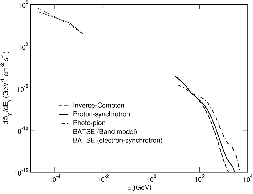
Figure 3 shows final spectra in the observer’s frame when both internal and intergalactic absorption are taken into account, assuming the burst is arriving from a redshift of (appropriate for GRB 971110). Even though the source spectra are vastly different, the observed high-energy gamma spectra are quite similar. Hence, the implied source energy requirement may be the only way to distinguish between the models. For illustration, Figure 3 also includes the observed BATSE spectrum for this burst, fit with both the Band (Eq. [1]) and electron-synchrotron models.
VII Results
In this work we use the muon observations of Project GRAND to fix the normalization (or upper limit) in each of the models described above for the various bursts analyzed. That is, the spectral shape is fixed from equations (40), (32), or (20), and the number of muons expected is then computed using
| (48) |
where is the collecting area of the Project GRAND array (the effective area at the time of GRB 971110 was approximately cm2), is the primary gamma-ray detection threshold for Project GRAND ( GeV), and is the probability per primary for a muon to reach detection level at Project GRAND. This probability (valid for GeV) was computed by Fasso & Poirier (2001) using the Monte Carlo atmospheric absorption code, FLUKA. Here includes both the internal and intergalactic optical depth estimated for each burst as described above. For illustration, Table 4 summarizes some estimates of the relative magnitudes of internal and intergalactic optical depths at two energy scales, 100 GeV and 1 TeV.
In practice, the integral in equation (48) is cut off at TeV since the optical depth is quite high for photons above this energy. The normalization constants for each model are then adjusted so that agrees with the upper limits set by Project GRAND, except for GRB 971110 where we used the observed mean value (see Table 1). Here we adopt typical values for the degree of equipartition and the relativistic Lorentz factor , namely and . Below we explore the dependence of our results on a broad range of these parameters.
We can then use our normalized gamma spectra to estimate the total energy emitted in high-energy gammas at the source. For the inverse-Compton model, we can also estimate the energy emitted in electrons, noting again the characteristic spectrum of a Fermi mechanism given in equation (9). Similarly we can estimate the energy emitted in protons for the proton-synchrotron and photo-pion models. Implied energies for photon emission into are given in Tables 5, 6, and 7 for the inverse-Compton, proton-synchrotron, and photo-pion models, respectively. We also list the required energies of the source protons or electrons, as appropriate. Our results assume for the accelerated electron and proton spectra. For GRB 971110 we estimated the statistical uncertainties of our results using Monte Carlo techniques to explore the parameter space of each of the models assuming Gaussian error distributions.
As evidenced by the large uncertainties, the models are not well constrained at present. Nevertheless, several points are worth noting from the tables. For the most significant possible detection (GRB 971110), the energetic requirements for the IC model ( erg) and the proton-synchrotron model ( erg) are much less than that for a photo-pion mechanism ( erg), as expected.
The distinction between the inverse-Compton and proton-synchrotron mechanisms has an important consequence on the magnetic field of the GRB, specifically the degree of equipartition, . In the case of inverse-Compton scattering, the ratio of the inverse-Compton luminosity to electron-synchrotron luminosity should be equal to the ratio of the IC target photon energy density to the magnetic field energy density since both mechanisms arise from the same population of hot relativistic electrons. Thus,
| (49) |
where and is the total rest-frame energy density of the emission region. If we adopt the generally accepted view that the MeV gamma rays seen by BATSE are caused by electron-synchrotron radiation then . For GRB 971110, , which implies
| (50) |
Since the energy density of the MeV BATSE gamma rays is likely to be higher than any other radiation source available for inverse-Compton scattering, we identify this energy density as . This association has been implicit throughout this paper. On the other hand, since the energy density of the TeV gamma rays must be greater than by about . We can then use as a lower limit for the total rest-frame energy density . Combining this with Eq. (50) we get the following upper limit on the degree of equipartition
| (51) |
Note also that Eq. (49) holds only in the classical regime. In the KN regime is even smaller because inverse-Compton scattering becomes less efficient. Hence, the inverse-Compton model is at odds with models that propose GRBs as the source of ultra-high energy cosmic rays, since those models require a magnetic field near equipartition, (cf. Waxman, 1995).
In Figures 4, 5, and 6 we explore the dependence of our results upon a broad range of possible values for , , and , respectively. These uncertainties were not formally included in our statistical estimates. Nevertheless, these figures support our qualitative conclusions. Specifically, the energetic requirements of all three models are in excess of that for the GRB for a broad range of parameters. Indeed most parameter variations in Figures 4 - 6 only exacerbate this problem. However, the inverse-Compton and proton-synchrotron mechanisms are generally less sensitive to changes in over the range or changes in over the range . The sharp increase in the energy content of the protons and electrons at small enters primarily through the internal optical depth. Figure 5 shows that the proton-synchrotron mechanism is highly efficient over a fairly broad range of ().
Regardless of the mechanism, if GRB 971110 is indeed a detection and our estimated redshift of is valid, the implied energy in energetic ( GeV) gamma rays is more than 100 times higher than the energy in the low-energy gamma rays. This renders the already challenging energetic requirements on the GRB source engine to be even more difficult. It may be possible to alleviate this difficulty if, perhaps, the photon beaming angle is much narrower for the high-energy component than for the low-energy GRB. Another possibility is that the redshift is much lower than our estimated value for this burst. In Figure 7 we explore the energetic requirements for GRB 971110 over a very broad range of redshifts from 0.005 to 3. This range is consistent with most currently measured GRB redshifts. This figure illustrates quite clearly the critical role that intergalactic absorption plays in driving up the energetic requirements and highlights the need for accurately determining the true redshifts of GRBs.
VIII Conclusion
We have analyzed the eight GRBs discussed in Poirier et al. (2003), which occurred above the Project GRAND array. We have studied the implied energies in energetic (TeV) gamma rays (and associated electrons and protons) of such GRBs in the context of three possible mechanisms: inverse-Compton scattering, proton-synchrotron radiation, and photo-pion production. Our analysis suggest that all of these models face significant energetic requirements. Gamma-ray production by either inverse-Compton scattering or proton-synchrotron radiation is probably the most efficient process.
Although it can not be claimed that TeV gammas have unambiguously been detected in association with low-energy GRBs, we have argued that there is enough mounting evidence to warrant further study. Furthermore, we have shown that if TeV gammas continue to be observed, then they present some interesting dilemmas for GRB physics. In view of their potential as a probe of the GRB source environment, we argue that further efforts to measure energetic gamma rays in association with low-energy gamma-ray bursts are warranted.
Acknowledgements.
The authors would like to thank M. S. Briggs for providing fits to these BATSE data. This research has made use of data obtained from the High Energy Astrophysics Science Archive Research Center, provided by NASA’s Goddard Space Flight Center. Project GRAND’s research is presently being funded through a grant from the University of Notre Dame and private grants. This work was supported in part by DoE Nuclear Theory grant DE-FG02-95ER40934 at the University of Notre Dame. This work was performed in part under the auspices of the US Department of Energy by the University of California, Lawrence Livermore National Laboratory under contract W-7405-Eng-48. One of the authors (TT) wishes to acknowledge support under a fellowship for research abroad provided by the Japanese Society for the Promotion of Science.References
- Schneid et al. (1992) Schneid, E. J., et al. 1992, Astron. Astrophys., 255, L13
- Hurley (1994) Hurley, K. 1994, Nature, 372, 652
- Catelli, Dingus, & Schneid (1997) Catelli, J. R., Dingus, B. L. & Schneid, E. J. 1997, in Gamma Ray Bursts, ed. C. A. Meegan (New York: AIP)
- Amenomori et al. (1996) Amenomori, M., et al. 1996, Astron. Astrophys., 311, 919
- Padilla et al. (1998) Padilla, L., et al. 1998, Astron. Astrophys., 337, 43
- Atkins et al. (2000) Atkins, R., et al. 2000, Astrophys. J., 533, L119
- Poirier et al. (2003) Poirier, J., D’Andrea, C., Fragile, P. C., Gress, J., Mathews, G. J., Race, D. 2003, Phys. Rev. D, 67, 042001
- Vernetto (2000) Vernetto, S. 2000, Astropart. Phys., 13, 75
- Salamon & Stecker (1998) Salamon, M. H. & Stecker, F. W. 1998, Astrophys. J., 493, 547
- Totani (2000) Totani, T. 2000, Astrophys. J., 536, L23
- Vietri (1997) Vietri, M. 1997, Phys. Rev. Lett., 78, 4328
- Totani (1998a) Totani, T. 1998a, Astrophys. J., 502, L13
- Totani (1998b) Totani, T. 1998b, Astrophys. J., 509, L81
- Waxman (1995) Waxman, E. 1995, Phys. Rev. Lett., 75, 386
- Waxman & Bahcall (1997) Waxman, E. & Bahcall, J. 1997, Phys. Rev. Lett., 78, 2292
- Garnavich et al. (2002) Garnavich, P., et al. 2002, BAS, 200, 2505
- Paczyński (1986) Paczyński, B. 1986, Astrophys. J., 308, L43
- Goodman (1986) Goodman, J. 1986, Astrophys. J., 308, L47
- Sari, Piran, & Narayan (1998) Sari, R., Piran, T., & Narayan, R. 1998, Astrophys. J., 497, L17
- Paczyński & Xu (1994) Paczyński, B. & Xu, G. 1994, Astrophys. J., 427, 708
- Mészáros & Rees (1994) Mészáros, P. & Rees, M. J. 1994, Mon. Not. R. Astron. Soc., 269, L41
- Rees & Mészáros (1992) Rees, M. & Mészáros, P. 1992, Mon. Not. R. Astron. Soc., 258, P41
- Vietri (1995) Vietri, M. 1995, Astrophys. J., 453, 883
- Böttcher & Dermer (1998) Böttcher M. & Dermer, C. D. 1998, Astrophys. J., 499, L131
- Band et al. (1993) Band, D. et al. 1993, Astrophys. J. 413, 281
- Kulkarni et al. (1999) Kulkarni, S. R., et al. 1999, Nature, 398, 389
- Fenimore & Ramirez-Ruiz (2000) Fenimore, E. E. & Ramirez-Ruiz, E. 2000, preprint(astro-ph/0004176) [Our analysis is based upon an early preprint of this paper. In later revisions the authors somewhat altered their equations from what is used in this work. Nevertheless, the earlier version is adequate for our purposes.]
- Garnavich et al. (1998) Garnavich, P. M., et al. 1998, Astrophys. J., 493, L53
- Perlmutter et al. (1998) Perlmutter, S., et al. 1998, Nature, 391, 51
- Freedman et al. (2001) Freedman, W. L., et al. 2001, Astrophys. J., 553, 47
- Reichart et al. (2001) Reichart, D. E., Lamb, D. Q., Fenimore, E. E., Ramirez-Ruiz, E., Cline, T. L., & Hurley, K. 2001, Astrophys. J., 522, 57
- Schaefer, Deng, & Band (2001) Schaefer, B. E., Deng, M. & Band, D. L. 2001, Astrophys. J., 563, L123
- Preece et al. (2000) Preece, R. D., Briggs, M. S., Mallozzi, R. S., Pendleton, G. N., Paciesas, W. S., & Band, D. L. 2000, Astrophys. J. Supp., 126, 19
- Zdziarski & Krolik (1993) Zdziarski, A. A. & Krolik, J. H. 1993, Astrophys. J., 409, L33
- Hillas (1984) Hillas, A. M. 1984, ARA&A, 22, 425
- Brumenthal & Gould (1970) Brumenthal, G. R. & Gould, R. J. 1970, Rev. Mod. Phys., 42, 237
- Salmonson, Wilson, & Mathews (2001) Salmonson, J., Wilson, J. R. & Mathews, G. J. 2001, Astrophys. J., 553, 471
- Sari & Esin (2001) Sari, R. & Esin, A. A. 2001, Astrophys. J., 548, 787
- Bird et al. (1994) Bird, D. J., et al. 1994, Astrophys. J., 424, 491
- Totani (1997) Totani, T. 1997, Astrophys. J., 486, L71
- Totani (1999) Totani, T. 1999, Astrophys. J., 511, 41
- Schmidt (1999) Schmidt, M. 1999, Astrophys. J., 523, L117
- Totani, Yoshii, & Sato (1997) Totani, T., Yoshii, Y., & Sato, K. 1997, Astrophys. J., 483, L75
- Hauser et al. (1998) Hauser, M. G., et al. 1998, Astrophys. J., 508, 25
- Primack et al. (1999) Primack, J. R., Bullock, J. S., Somerville, R. S., & MacMinn, D. 1999, Astropart. Phys., 11, 93
- Fasso & Poirier (2001) Fasso, A. & Poirier, J. 2001, Phys. Rev. D, 63, 036002 (2001)


| GRB | Trig | T90111Angles RA, Dec, and in degrees and T90 in seconds. | RA111Angles RA, Dec, and in degrees and T90 in seconds. | Dec111Angles RA, Dec, and in degrees and T90 in seconds. | 111Angles RA, Dec, and in degrees and T90 in seconds. | 222Upper limits are confidence level. |
|---|---|---|---|---|---|---|
| 971110 | 6472 | 195.2 | 242 | 50 | 0.6 | |
| 990123 | 7343 | 62.5 | 229 | 42 | 0.4 | |
| 940526 | 2994 | 48.6 | 132 | 34 | 1.7 | |
| 980420 | 6694 | 39.9 | 293 | 27 | 0.6 | |
| 960428 | 5450 | 172.2 | 304 | 35 | 1.0 | |
| 980105 | 6560 | 36.8 | 37 | 52 | 1.4 | |
| 980301 | 6619 | 36.0 | 148 | 35 | 1.3 | |
| 970417a | 6188 | 7.9 | 290333RA, Dec, and for GRB 970417a are based upon the Milagrito data. | 54333RA, Dec, and for GRB 970417a are based upon the Milagrito data. | 0.5333RA, Dec, and for GRB 970417a are based upon the Milagrito data. |
| GRB | (cm-2 s-1 MeV-1) | (MeV) | (s) | ||
|---|---|---|---|---|---|
| 971110 | 1.8 | ||||
| 990123 | 4.1 | ||||
| 940526 | 1.2 | ||||
| 980420 | 1.8 | ||||
| 960428 | 0.7 | ||||
| 980105 | 1.2 | ||||
| 980301 | 2.3 | ||||
| 970417a | 111Spectral fits were not available for GRB 970417a. Properties are based upon assumed redshift , observed BATSE fluence, and average GRB spectral shape. | 222Average parameters for all bright GRBs considered in Preece et al. (2000). | 222Average parameters for all bright GRBs considered in Preece et al. (2000). | 222Average parameters for all bright GRBs considered in Preece et al. (2000). | 1.1 |
| 111Available at http://www.batse.msfc.nasa.gov/batse/ | 222The redshift uncertainties are crudely estimated as from the variability-luminosity relation. | 333We quote the isotropic luminosities. These must be multiplied by to get the true luminosities. | 333We quote the isotropic luminosities. These must be multiplied by to get the true luminosities. | ||
|---|---|---|---|---|---|
| GRB | (photons cm-2 s-1) | (erg s-1) | (erg s-1) | ||
| 971110 | 0.0204 | ||||
| 990123 | 0.0113 | 1.6444Kulkarni et al. (1999) | |||
| 940526 | 0.0175 | ||||
| 980420 | 0.0267 | ||||
| 960428 | 0.0628 | ||||
| 980105 | 0.0671 | ||||
| 980301 | 0.0232 | ||||
| 970417a555GRB 970417a was too weak in the BATSE band to apply the variability-luminosity relation. | 666Totani (2000). |
| Internal Optical Depth | Intergalactic Optical Depth | ||||
|---|---|---|---|---|---|
| GRB | GeV | 1 TeV | GeV | 1 TeV | |
| 971110 | |||||
| 990123 | 111Large uncertainties in the fit parameters made constraints on the internal optical depth uninformative in these cases. For these bursts, we have made the optimistic assumption | 111Large uncertainties in the fit parameters made constraints on the internal optical depth uninformative in these cases. For these bursts, we have made the optimistic assumption | 2.8 | 31. | |
| 940526 | 111Large uncertainties in the fit parameters made constraints on the internal optical depth uninformative in these cases. For these bursts, we have made the optimistic assumption | 111Large uncertainties in the fit parameters made constraints on the internal optical depth uninformative in these cases. For these bursts, we have made the optimistic assumption | |||
| 980420 | 111Large uncertainties in the fit parameters made constraints on the internal optical depth uninformative in these cases. For these bursts, we have made the optimistic assumption | 111Large uncertainties in the fit parameters made constraints on the internal optical depth uninformative in these cases. For these bursts, we have made the optimistic assumption | |||
| 960428 | 111Large uncertainties in the fit parameters made constraints on the internal optical depth uninformative in these cases. For these bursts, we have made the optimistic assumption | 111Large uncertainties in the fit parameters made constraints on the internal optical depth uninformative in these cases. For these bursts, we have made the optimistic assumption | |||
| 980105 | 111Large uncertainties in the fit parameters made constraints on the internal optical depth uninformative in these cases. For these bursts, we have made the optimistic assumption | 111Large uncertainties in the fit parameters made constraints on the internal optical depth uninformative in these cases. For these bursts, we have made the optimistic assumption | |||
| 980301 | 111Large uncertainties in the fit parameters made constraints on the internal optical depth uninformative in these cases. For these bursts, we have made the optimistic assumption | 111Large uncertainties in the fit parameters made constraints on the internal optical depth uninformative in these cases. For these bursts, we have made the optimistic assumption | |||
| 970417a | 111Large uncertainties in the fit parameters made constraints on the internal optical depth uninformative in these cases. For these bursts, we have made the optimistic assumption | 111Large uncertainties in the fit parameters made constraints on the internal optical depth uninformative in these cases. For these bursts, we have made the optimistic assumption | |||
| 111We quote the isotropic energies. These entries must be multiplied by to get the true energies. | 111We quote the isotropic energies. These entries must be multiplied by to get the true energies. | |||||
|---|---|---|---|---|---|---|
| GRB | (cm-2 s-1 GeV-1) | (GeV) | (GeV) | (GeV) | (erg) | (erg) |
| 971110 | ||||||
| 990123 | 0.04 | 2.8 | 23. | |||
| 940526 | 14. | 7.3 | 5.1 | |||
| 980420 | 0.3 | 9.8 | 56. | |||
| 960428 | 0.004 | 8.2 | 380 | |||
| 980105 | 0.04 | 17. | 350 | |||
| 980301 | 0.05 | 6.5 | 73. | |||
| 970417a | 8.6 | 33. | 63. |
Here we estimate the total energy escaping in the gamma-ray component from each burst using the inverse-Compton model. We also estimate the total energy in the electron component at the source.
| 111We quote the isotropic energies. These entries must be multiplied by to get the true energies. | 111We quote the isotropic energies. These entries must be multiplied by to get the true energies. | |||
|---|---|---|---|---|
| GRB | (cm-2 s-1 GeV-1) | (GeV) | (erg) | (erg) |
| 971110 | ||||
| 990123 | ||||
| 940526 | ||||
| 980420 | ||||
| 960428 | ||||
| 980105 | ||||
| 980301 | ||||
| 970417a |
Here we estimate the total energy escaping in the gamma-ray component from each burst using the proton-synchrotron model. We also estimate the total energy in the proton component at the source.
| 111We quote the isotropic energies. These entries must be multiplied by to get the true energies. | 111We quote the isotropic energies. These entries must be multiplied by to get the true energies. | |||
|---|---|---|---|---|
| GRB | (cm-2 s-1 GeV-1) | ( GeV) | (erg) | (erg) |
| 971110 | ||||
| 990123 | 1.5 | |||
| 940526 | 4.0 | |||
| 980420 | 5.3 | |||
| 960428 | 4.4 | |||
| 980105 | 9.4 | |||
| 980301 | 3.5 | |||
| 970417a | 18. |
Here we estimate the total energy escaping in the gamma-ray component from each burst using the photo-pion model. We also estimate the total energy in the proton component at the source.