11institutetext: SISSA/ISAS, Trieste - V. Beirut 2-4, 34014
22institutetext: Osservatorio Astronomico di Brera, via Bianchi 46, Merate (LC), Italy

Time Resolved Spectral Analysis of Bright Gamma Ray Bursts

G. Ghirlanda 11    A. Celotti 11    G. Ghisellini 22
(21 June 2002)

We present the time integrated and time resolved spectral analysis of a sample of bright bursts selected with $F_{peak}\geq 20\ \mathrm{phot\ cm^{-2}\ sec^{-1}}$ from the BATSE archive. We fitted four different spectral models to the pulse time integrated and time resolved spectra. We compare the low energy slope of the fitted spectra with the prediction of the synchrotron theory [predicting photon spectra softer than $N(E)\propto E^{-2/3}$], and test, through direct spectral fitting, the synchrotron shock model. We point out that differences in the parameters distribution can be ascribed to the different spectral shape of the models employed and that in most cases the spectrum can be described by a smoothly curved function. The synchrotron shock model does not give satisfactory fits to the time averaged and time resolved spectra. Finally, we derive that the synchrotron low energy limit is violated in a considerable number of spectra both during the rise and decay phase around the peak.

Key Words.:
Gamma Rays:bursts – methods:data analysis – radiation mechanisms:non–thermal
offprints: G. Ghirlanda; email: ghirland@sissa.it

1 Introduction

The nature and emission mechanisms responsible for the prompt emission of Gamma–ray bursts (GRB) are still a matter of debate. From the phenomenological perspective much effort has been made in order to characterize and identify typical spectral properties of bursts, mostly by applying parametric but very general and simple spectral models. Probably the most widely adopted is that suggested by Band et al. (Band b (1993)), namely a smoothly connected double power law model. Its attractive feature is that it characterizes, within the observational energy window, the most relevant quantities, namely the peak energy, representing the energy at which most of the emission occurs, and the low and high energy components which are related, according to the most accredited emission theories, to the particle energy distribution and/or to the physical parameters of the emitting region. Indeed GRB spectra result to be well represented by the Band parameterization ($N(E)\propto E^{\alpha,\beta}$), with typical low energy power law photon spectral indices $\alpha$ between –1.25 and –0.25, high energy spectral indices $\beta$ around –2.25 (Preece et al. Preece1998 (1998)) and peak energy $E_{p}$ typically around 100–300 keV.

A fundamental issue in the spectral analysis of GRBs is the integration timescale of the spectra which are observed to vary even on millisecond timescales (Fishman et al. 1995b ). BATSE spectra, which are integrated for a minimum of 128ms, therefore represent the best way, presently available, to constrain the burst emission mechanism. Furthermore, in order to compare the average spectral properties of different bursts, also time integrated spectra, covering the duration of the pulse or the entire burst, have been used in literature.

It has been found in general that the Band model not only well describes the time integrated spectra, but it also appears to fit the time resolved spectra of bright bursts. Alternative spectral models – and in particular the predictions for synchrotron emission (Katz Katz (1994), Crider at al. 1997a ,b) – have also been recently tested on a large sample of time resolved spectra by Preece and collaborators (Preece et al. Preece2000 (2000)).

Within this scenario, here we present the study of the spectral properties of single pulses within bright GRBs which intends to complement the work mentioned above, by specifically aiming at: 1) compare the results of the analysis of the spectra averaged over major pulses in the burst lightcurve with the time resolved spectra of the very same burst in order to quantify systematic differences; 2) consider both empirical (Band model) and more ‘physical’ (synchrotron shock model) spectral models for all spectra and compare the quality of the corresponding fits. In particular each spectrum is fitted with the four models we choose (Band’s, broken power–law, thermal Comptonization and synchrotron shock model, the latter fitted to temporal resolved BATSE spectra for the first time). We also examine any spectral ‘violation’ (with respect to the predicted slope in the case of synchrotron emission) for the entire burst evolution. The development of this work is the analysis and interpretation of the spectral evolution morphologies of this sample of bursts.

The paper is structured as follows: In sect. 2 we describe the data and their selection criteria, while the spectral models adopted for the analysis are detailed in sect. 3. Section 4 presents the results of our work for the time integrated and time resolved spectra. Conclusions are drawn in sect. 5. The time evolution of the spectral parameter will be the content presented in a following paper (Ghirlanda et al. in preparation).

2 Data selection and analysis

2.1 Instrumental summary

The Burst and Transient Source Experiment (BATSE) consisted of eight detection modules on the corners of the Compton Gamma Ray Observatory (CGRO – deorbited in summer 2001). Each module was composed by two instruments: the Large Area Detector (LAD) designed for burst location and temporal analysis, and the Spectroscopic Detector (SD) suited for spectral study.

Each LAD consisted of a thin circular NaI layer of 2025 $cm^{2}$ collecting area. The nominal energy coverage was 28 – 1800 keV (with minor variations between different detector modules). The energy resolution was about 20% at 511 keV (Fishman et al. 1989a ).

The SDs were smaller (127 $cm^{2}$) but thicker and thus had a greater energy conversion efficiency. Their sensitive energy range varied with the gain settings and energy thresholds of the photomultipliers, but typically extended from 20 keV to 2 MeV (Band et al. Band a (1992)). The energy resolution is 7% at 662 keV (Fishman et al. 1989a , Band et al. Band b (1993)).

After a burst trigger, during the following 4 minutes burst mode, the LADs accumulated, among other data products, the High Energy Resolution Burst (HERB) spectra. These data are a sequence of 128 quasi–logarithmically spaced energy channel spectra with a maximum time resolution of 128 ms. They were accumulated from the 4 most illuminated detectors. The SDs produced similar spectra with 256 energy channels and 128 ms resolution (SHERB). The maximum number of spectra accumulated is 128 and 192 for the HERB and SHERB data, respectively. The LAD and SD spectral time integration algorithm was based on a count rate criterion so that the instruments provided spectra with a minimum integration time of 128 ms only for particularly intense bursts or around the peaks, while in most cases the spectral accumulation timescale was much greater than 128 ms.

2.2 Data Selection

The HERB data have been systematically preferred for this work because the higher detection area of the LAD ensures an higher count rate than the SD detectors. Despite their moderate energy resolution (if compared to the SDs) they are suited for the continuum spectral study (Preece et al. Preece2000 (2000)).

There are a few cases (see col. 3 in Table 1) for which the SHERB data were used because there were telemetry gaps.

We have analyzed the HERB data from rank 1 detector. The rank of the detector (col. 4 in Table 1) is an indication of the relative count rate during the trigger: rank 1 detector has the highest count rate, the best S/N and the highest spectral time resolution. For the SHERB data the detector choice is a compromise between the highest degree of illumination (the first rank SD detector) and the highest gain which depends on different ground setting parameters, which have been changed during the mission (Band D., private communication). The gain of the photomultiplier, in fact, scales the spectrum up or down in energy: the highest is the gain the more the detector is sensible to the low energy photons and the lower is the low energy threshold (Preece et al., Preece b (1996); Kitchin Kitchin (1991)). We selected the highest rank SD detector with the 511 keV calibration line centroid above uncompressed channel 800.

2.3 The bursts sample

The bursts were selected from the BATSE 4B catalog111http://cossc.gsfc.nasa.gov/batse/4Bcatalog/index.html. which is complete until 29 Aug 1996 (trigger 5586). This catalog was complemented with the on line catalog which includes the triggers after 5586 until trigger 8121 (9 Sept 2000).

We have selected GRBs with a peak flux on the 64 ms time scale (calculated according to Fishman et al. Fishman1 (1994), Meegan et al. Meegan1 (1996), Paciesas et al. Paciesas (1999)) higher than 20 $\mathrm{phot\ cm^{-2}\ sec^{-1}}$. This choice is motivated by the fact that bright bursts should provide time resolved spectra with good S/N (also on integration of the order of 128 ms). We collected in this way 38 bursts whose trigger number, name and peak flux are reported in Table. 1 (cols. 1, 2 and 6, respectively).

The sample selected according to the peak flux criterion was reduced during the spectral analysis because of data problems (trigger 1609, 1711, 3480) or because the number of spectra available for the spectral analysis was less than 5 (trigger 1997, 2151, 2431, 2611, 3412, 5711, 5989, 6293, 6904, 7647). This happened particularly in short bursts which have typical duration lower than 1 second. The bursts which were not analyzed have dashes entries in tab 1. The final sample of analyzed bursts contains 25 bursts and is obviously not complete with respect to the flux selection criterion. All the analyzed bursts except trigger 5563,7301,7549 are also present in Preece et al. (Preece2000 (2000)) spectral sample.

Table 1: The GRB sample
TriggeraGRBDataDetectorPeakFluxcBackgroundPeakeSpectrafS/NgTypebNumberRank[phot/cm2/sec]#dnd143910503HERBLAD6152.08±1.43834491473920311HERBLAD5125.31±0.7623551541920406SHERBSD2238.32±0.89521915160992051767.59±1.211625920525HERBLAD4128.06±0.7484325171192072021.7±0.7199792102240.33±0.852083921207HERBLAD0146.55±0.92622312151930131167.84±2.632329930506SHERBSD2442.57±0.90114142243193070643.83±0.892537930922HERBLAD1127.28±0.731432345261193103135.05±0.892798940206HERBLAD3124.19±0.73731162831940217HERBLAD0144.34±1.08104328341295021154.82±0.76348095032521.61±0.513481950325HERBLAD2125.7±0.6643273491950403HERBLAD3130.65±0.6263344453492950403HERBLAD5161.44±0.9164122453523950425HERBLAD6121.81±0.53422504368960114SHERBSD0158.61±0.8384329455477960529HERBLAD1129.35±0.70742125563960804HERBLAD4122.7±0.5974185567960807HERBLAD0122.8±0.664525455614960924SHERBSD61183.37±1.621241225621961001HERBLAD2125.64±0.613142175704961202HERBLAD0143.93±0.76264113571196121241.25±0.71598997020177.61±0.896198970420HERBLAD4166.5±0.9124138629397070488.53±1.6404970930HERBLAD6124.01±0.522142226581980125HERBLAD0140.91±0.69154117690498070654.62±0.877301990104HERBLAD7186.53±0.931245247549990506HERBLAD7125.12±0.5894652764799071224.06±0.51missing-subexpressionmissing-subexpressionmissing-subexpressionmissing-subexpressionmissing-subexpressionmissing-subexpressionmissing-subexpressionmissing-subexpressionmissing-subexpressionmissing-subexpressionmissing-subexpressionmissing-subexpression𝑇𝑟𝑖𝑔𝑔𝑒𝑟superscripta𝐺𝑅𝐵𝐷𝑎𝑡𝑎𝐷𝑒𝑡𝑒𝑐𝑡𝑜𝑟𝑃𝑒𝑎𝑘𝐹𝑙𝑢𝑥superscriptc𝐵𝑎𝑐𝑘𝑔𝑟𝑜𝑢𝑛𝑑𝑃𝑒𝑎𝑘superscripte𝑆𝑝𝑒𝑐𝑡𝑟𝑎superscriptf𝑆𝑁superscriptgmissing-subexpressionmissing-subexpression𝑇𝑦𝑝𝑒superscriptb𝑁𝑢𝑚𝑏𝑒𝑟𝑅𝑎𝑛𝑘delimited-[]𝑝𝑜𝑡𝑐superscript𝑚2𝑠𝑒𝑐#superscriptd𝑛superscriptdmissing-subexpressionmissing-subexpressionmissing-subexpressionmissing-subexpressionmissing-subexpressionmissing-subexpressionmissing-subexpressionmissing-subexpressionmissing-subexpressionmissing-subexpressionmissing-subexpressionmissing-subexpressionmissing-subexpressionmissing-subexpressionmissing-subexpression143910503𝐻𝐸𝑅𝐵𝐿𝐴𝐷61plus-or-minus52.081.43834491473920311𝐻𝐸𝑅𝐵𝐿𝐴𝐷51plus-or-minus25.310.7623551541920406𝑆𝐻𝐸𝑅𝐵𝑆𝐷22plus-or-minus38.320.895219151609920517plus-or-minus67.591.211625920525𝐻𝐸𝑅𝐵𝐿𝐴𝐷41plus-or-minus28.060.74843251711920720plus-or-minus21.70.71997921022plus-or-minus40.330.852083921207𝐻𝐸𝑅𝐵𝐿𝐴𝐷01plus-or-minus46.550.92622312151930131plus-or-minus167.842.632329930506𝑆𝐻𝐸𝑅𝐵𝑆𝐷24plus-or-minus42.570.901141422431930706plus-or-minus43.830.892537930922𝐻𝐸𝑅𝐵𝐿𝐴𝐷11plus-or-minus27.280.7314323452611931031plus-or-minus35.050.89missing-subexpressionmissing-subexpressionmissing-subexpressionmissing-subexpressionmissing-subexpression2798940206𝐻𝐸𝑅𝐵𝐿𝐴𝐷31plus-or-minus24.190.73731162831940217𝐻𝐸𝑅𝐵𝐿𝐴𝐷01plus-or-minus44.341.081043283412950211plus-or-minus54.820.763480950325plus-or-minus21.610.513481950325𝐻𝐸𝑅𝐵𝐿𝐴𝐷21plus-or-minus25.70.6643273491950403𝐻𝐸𝑅𝐵𝐿𝐴𝐷31plus-or-minus30.650.6263344453492950403𝐻𝐸𝑅𝐵𝐿𝐴𝐷51plus-or-minus61.440.9164122453523950425𝐻𝐸𝑅𝐵𝐿𝐴𝐷61plus-or-minus21.810.53422504368960114𝑆𝐻𝐸𝑅𝐵𝑆𝐷01plus-or-minus58.610.8384329455477960529𝐻𝐸𝑅𝐵𝐿𝐴𝐷11plus-or-minus29.350.70742125563960804𝐻𝐸𝑅𝐵𝐿𝐴𝐷41plus-or-minus22.70.5974185567960807𝐻𝐸𝑅𝐵𝐿𝐴𝐷01plus-or-minus22.80.664525455614960924𝑆𝐻𝐸𝑅𝐵𝑆𝐷61plus-or-minus183.371.621241225621961001𝐻𝐸𝑅𝐵𝐿𝐴𝐷21plus-or-minus25.640.613142175704961202𝐻𝐸𝑅𝐵𝐿𝐴𝐷01plus-or-minus43.930.762641135711961212plus-or-minus41.250.715989970201plus-or-minus77.610.896198970420𝐻𝐸𝑅𝐵𝐿𝐴𝐷41plus-or-minus66.50.91241386293970704formulae-sequenceplus-or-minus88.5316404970930𝐻𝐸𝑅𝐵𝐿𝐴𝐷61plus-or-minus24.010.522142226581980125𝐻𝐸𝑅𝐵𝐿𝐴𝐷01plus-or-minus40.910.691541176904980706plus-or-minus54.620.877301990104𝐻𝐸𝑅𝐵𝐿𝐴𝐷71plus-or-minus86.530.931245247549990506𝐻𝐸𝑅𝐵𝐿𝐴𝐷71plus-or-minus25.120.58946527647990712plus-or-minus24.060.51missing-subexpression{\scriptsize\begin{array}[]{ccccccccccc}\hline\cr\vskip 3.0pt plus 1.0pt minus 1.0pt\cr Trigger$$^{\mathrm{a}}$$&GRB&Data&\lx@intercol\hfil Detector\hfil\lx@intercol&PeakFlux$$^{\mathrm{c}}$$&\lx@intercol\hfil Background\hfil\lx@intercol&Peak$$^{\mathrm{e}}$$&Spectra$$^{\mathrm{f}}$$&S/N$$^{\mathrm{g}}$$\\ &&Type$$^{\mathrm{b}}$$&Number&Rank&[phot/cm^{2}/sec]&\#$$^{\mathrm{d}}$$&n$$^{\mathrm{d}}$$&&&$$\geq$$\\ \vskip 3.0pt plus 1.0pt minus 1.0pt\cr\hline\cr\vskip 3.0pt plus 1.0pt minus 1.0pt\cr 143&\object{910503}&HERB&LAD6&1&$$52.08\pm 1.43$$&8&3&4&49&-\\ 1473&\object{920311}&HERB&LAD5&1&$$25.31\pm 0.7$$&6&2&3&55&-\\ 1541&\object{920406}&SHERB&SD2&2&$$38.32\pm 0.89$$&5&2&1&9&15\\ 1609&920517&--&--&-&$$67.59\pm 1.21$$&-&-&-&-&-\\ 1625&\object{920525}&HERB&LAD4&1&$$28.06\pm 0.74$$&8&4&3&25&-\\ 1711&920720&--&--&-&$$21.7\pm 0.7$$&-&-&-&-&-\\ 1997&921022&--&--&-&$$40.33\pm 0.85$$&-&-&-&-&-\\ 2083&\object{921207}&HERB&LAD0&1&$$46.55\pm 0.92$$&6&2&2&31&-\\ 2151&930131&--&--&-&$$167.84\pm 2.63$$&-&-&-&-&-\\ 2329&\object{930506}&SHERB&SD2&4&$$42.57\pm 0.90$$&11&4&1&42&-\\ 2431&930706&--&--&-&$$43.83\pm 0.89$$&-&-&-&-&-\\ 2537&\object{930922}&HERB&LAD1&1&$$27.28\pm 0.7$$&31&4&3&23&45\\ 2611&931031&--&--&-&$$35.05\pm 0.89$$&&&&&\\ 2798&\object{940206}&HERB&LAD3&1&$$24.19\pm 0.73$$&7&3&1&16&-\\ 2831&\object{940217}&HERB&LAD0&1&$$44.34\pm 1.08$$&10&4&3&28&-\\ 3412&950211&--&--&-&$$54.82\pm 0.76$$&-&-&-&-&-\\ 3480&950325&--&--&-&$$21.61\pm 0.51$$&-&-&-&-&-\\ 3481&\object{950325}&HERB&LAD2&1&$$25.7\pm 0.6$$&6&4&3&27&-\\ 3491&\object{950403}&HERB&LAD3&1&$$30.65\pm 0.62$$&6&3&3&44&45\\ 3492&\object{950403}&HERB&LAD5&1&$$61.44\pm 0.91$$&6&4&1&22&45\\ 3523&\object{950425}&HERB&LAD6&1&$$21.81\pm 0.53$$&4&2&2&50&-\\ 4368&\object{960114}&SHERB&SD0&1&$$58.61\pm 0.83$$&8&4&3&29&45\\ 5477&\object{960529}&HERB&LAD1&1&$$29.35\pm 0.70$$&7&4&2&12&-\\ 5563&\object{960804}&HERB&LAD4&1&$$22.7\pm 0.59$$&7&4&1&8&-\\ 5567&\object{960807}&HERB&LAD0&1&$$22.8\pm 0.6$$&6&4&5&25&45\\ 5614&\object{960924}&SHERB&SD6&1&$$183.37\pm 1.62$$&12&4&1&22&-\\ 5621&\object{961001}&HERB&LAD2&1&$$25.64\pm 0.61$$&31&4&2&17&-\\ 5704&\object{961202}&HERB&LAD0&1&$$43.93\pm 0.76$$&26&4&1&13&-\\ 5711&961212&--&--&-&$$41.25\pm 0.71$$&-&-&-&-&-\\ 5989&970201&--&--&-&$$77.61\pm 0.89$$&-&-&-&-&-\\ 6198&\object{970420}&HERB&LAD4&1&$$66.5\pm 0.9$$&12&4&1&38&-\\ 6293&970704&--&--&-&$$88.53\pm 1.$$&-&-&-&-&-\\ 6404&\object{970930}&HERB&LAD6&1&$$24.01\pm 0.52$$&21&4&2&22&-\\ 6581&\object{980125}&HERB&LAD0&1&$$40.91\pm 0.69$$&15&4&1&17&-\\ 6904&980706&--&--&-&$$54.62\pm 0.87$$&-&-&-&-&-\\ 7301&\object{990104}&HERB&LAD7&1&$$86.53\pm 0.93$$&12&4&5&24&-\\ 7549&\object{990506}&HERB&LAD7&1&$$25.12\pm 0.58$$&9&4&6&52&-\\ 7647&990712&--&--&-&$$24.06\pm 0.51$$&-&-&-&-&-\\ \vskip 3.0pt plus 1.0pt minus 1.0pt\cr\hline\cr\end{array}}
  • a

    Burst reference number from the Gamma Burst Catalog at
    $http://gammaray.msfc.nasa.gov/batse/grb/catalog/current/$

  • b

    (S)HERB: (Spectroscopic) High Energy Resolution Burst data.

  • c

    Peak flux on the 64 ms time-scale, integrated over the 50 - 300 keV energy range.

  • d

    Background is calculated on ” # ” number of spectra and with a polynomial function of degree ”n”.

  • e

    Number of pulses spectroscopically analyzed within each burst.

  • f

    Number of time resolved spectra per burst.

  • g

    S/N method used in grouping the time resolved spectra accumulated by the instrument.

Refer to caption
Figure 1: Example of light curve (trigger 2083). Each time bin represents the count rate summed over all the detectors that triggered, integrated in energy from 28 to 1800 keV and over the detection area (for details see Preece et al. Preece2000 (2000)). The line–filled regions show the time intervals of the average pulse spectrum accumulation. The start and stop times were chosen to have the same flux level. Our analysis is limited to the dashed areas, and therefore excludes the long slowly decaying part of the burst.

3 Spectral analysis

The spectral analysis has been performed with the software SOAR v3.0 (Spectroscopic Oriented Analysis Routines) by Ford (Ford (1993)). The power of this software is its multi–level routine structure which can be easily modified by the user: we implemented the spectral library with the broken power law and added the possibility of fitting each time resolved spectrum with a different energy binning scheme. The main capabilities of SOAR are: the possibility of analyzing HERB and SHERB data and rebinning (in time) spectra in different fashions (according to a fixed number of spectra per group or with a S/N ratio criterion). It is also possible to simulate burst spectra and spectral evolution (Ford Ford (1993)).

We used the package XSPEC, as widely used for high energy data, to test, for two bursts, the spectral analysis procedure. We found, within parameters errors, similar results. Any difference can be ascribed to a different background calculation technique.

The spectral analysis procedure consisted in the inspection of the light curve, i.e. the count rate in cts s-1 over the nominal energy band (typically 28–1800 keV) with each time bin corresponding to a time resolved spectrum (with typical integration time of 128 ms).

The background is calculated on a time interval as close as possible to the burst, but not contaminated by the burst itself. Typically we use a $1000\ \mathrm{sec}$ interval before and after the GRB, and fit the spectra contained in this interval with a polynomial background model examining the residuals for any systematic problem. The background spectrum to be subtracted is obtained by extrapolating the polynomial best fit spectrum, for every channel, in the time interval occupied by the burst. As reported in Table 1, in most cases the degree of the polynomial is 4.

The GRB light curve was used to identify the pulses as those structures in which the flux rises above and decays back to the background level. We accumulated the time resolved spectra within this time interval: this defines the time average pulse spectrum. In those pulses composed by several substructures we treated them separately only if their flux starts and returns to the background level and if they are separated by at least a 128ms time bin. In the example trigger of Fig. 1 we accumulated two average pulse spectra, corresponding to the dashed regions in the plot. The time averaged pulse spectrum was then fitted with the 4 spectral models described in the following section. The best fit results of the average spectrum were used as initial parameters guess for fitting the time resolved spectra.

For the time resolved spectra we used, as integration time, at first the shortest time available (i.e. 128 ms, at best), again limiting our analysis to the same time–span selected for the time integrated analysis. The best fit parameters were then examined in search for any indetermination: when at least 3 subsequent spectra had one or more undetermined spectral parameter, the spectra were grouped according to a S/N criterion. We followed the prescriptions of Preece et al. (Preece2000 (2000)) who accumulate subsequent HERB spectra until the S/N (calculated for the 28–1800 keV energy range) is greater than 45; for the SHERB data the S/N threshold was fixed at 15 as already done by Ford et al. (Ford a (1995)). If after this accumulation the number of time resolved spectra was less than 5 the burst was not included in the final list of analyzed events (see sect.2.2).

The spectra were also rebinned in energy in order to be confident that the Poisson statistic is represented by a normal distribution in every channel for the application of the $\chi^{2}$ minimization technique. We fixed the minimum number of counts per energy bin at 30 and 15 for the HERB and SHERB data, respectively.

3.1 Spectral Models

We used four spectral representations to fit the GRB time averaged and time resolved spectra. These functions were chosen in order to find whether a specific model can be considered as best representation of the spectral characteristics of pulses in bright GRBs. We explicitly exclude a fifth spectral model proposed in the literature by Ryde (Ryde (1999)) because it has a higher number of free parameters.

3.1.1 The Band model

This empirical model (BAND hereafter) was first proposed by Band et al. (Band b (1993)) and, as already mentioned, is a good general and simple description of the time averaged (Band et al.Band b (1993)) and the time resolved spectra (Ford et al Ford a (1995); Preece et al. Preece1998 (1998)). It contains the two continuum components in the keV–MeV band already discovered before BATSE: (i) a low energy power law with an exponential cutoff $N(E)\propto E^{\alpha}exp(-E/E_{0})$ and (ii) a high energy power law $N(E)\propto E^{\beta}$ (Matz et al. Matz (1985)). In fact the BAND model consists of 2 power laws joined smoothly by an exponential roll–over, namely:

$$N(E)=\left\{\begin{array}[]{l}A\left(\frac{E}{100\ \mathrm{keV}}\right)^{\alpha}\exp\left(-{E\over E_{0}}\right)\\ \hskip 105.0pt\mathrm{for}\ E\leq\left(\alpha-\beta\right)E_{0}\\ AE^{\beta}\left[\frac{(\alpha-\beta)E_{0}}{100\ \mathrm{keV}}\right]^{\alpha-\beta}\exp(\beta-\alpha)\\ \hskip 105.0pt\mathrm{for}\ E\geq\left(\alpha-\beta\right)E_{0}\end{array}\right.$$ (1)

where $N(E)$ is in photons cm-2 s-1 keV-1. The free parameters, which are the result of the fits, are:

  • A: the normalization constant @ 100 keV;

  • $\alpha$: the low energy power law spectral index;

  • $\beta$: the high energy power law spectral index;

  • $E_{0}$: the break energy, which represents the e–folding parameter.

If $\beta<-2$ the peak energy in the $E\ F_{E}$ diagram ($F_{E}$ is the flux in keV/$\mathrm{cm^{-2}sec^{-1}}$ keV) is $E_{peak}=(\alpha+2)E_{0}$ and represents the energy at which most of the power is emitted.

For the fitting procedure we had to assume an interval for the parameters and we fixed [$-5$,1] for $\alpha$ and $\beta$ and the break energy was allowed to vary in the range [28–1800] keV.

3.1.2 The Broken Power Law model

This model, called BPLW, is the simplest model used for fitting GRB spectra: it consists of two power laws sharply connected, with no curvature. Its analytical form is:

$$N(E)=\left\{\begin{array}[]{lll}AE^{\alpha}&\mathrm{for}&E\leq\left(\alpha-\beta\right)E_{0}\\ AE_{0}^{\alpha-\beta}E^{\beta}&\mathrm{for}&E\geq\left(\alpha-\beta\right)E_{0}\end{array}\right.$$ (2)

The free parameters are as before. In this model the peak energy of the $EF_{E}$ diagram coincides with the break energy $E_{0}$ for $\beta<-2$.

3.1.3 The Comptonization model

This spectral representation (COMP hereafter) is composed of a power law ending-up in an exponential cutoff, thus fitting well those spectra with a very steep high energy decline:

$$N(E)=AE^{\alpha}\exp\left(-\frac{E}{E_{0}}\right).$$ (3)

The free parameters are as in the previous models without the high energy component. In fact the COMP model can be analytically obtained from the BAND model assuming $\beta=-\infty$. This model might be considered to mimic the spectrum resulting from multiple Compton emission from a thermal medium.

3.1.4 The Synchrotron Shock Model

The model (SSM) is based on optically thin synchrotron emission from relativistic particles (either electrons and/or electron–positron pairs) (Tavani Tavani b (1996)). The electron energy distribution $N(\gamma)$, which is a relativistic Maxwellian before the shock occurs, is modeled for the internal shock passage by adding a high energy powerlaw component (Tavani Tavani b (1996)):

$$N\left(\gamma\right)\propto\left\{\begin{array}[]{lll}\frac{\gamma^{2}}{\gamma_{\star}^{3}}\exp\left(-\frac{\gamma}{\gamma_{\star}}\right)&\mathrm{for}&\frac{\gamma}{\gamma_{\star}}\leq 1\\ \gamma^{-\delta}&\mathrm{for}&1\leq\frac{\gamma}{\gamma_{\star}}\leq\frac{\gamma_{max}}{\gamma_{\star}}\end{array}\right.$$ (4)

where $\gamma m_{e}c^{2}$ is the electron energy, $\gamma_{\star}=k_{B}T^{\star}/m_{e}c^{2}$ is the pre-shock equilibrium electron energy, $\gamma^{-\delta}$ is the supra-thermal component and $\gamma_{max}$ is the maximum electron energy. The power law part of $N(\gamma)$ (of index $\delta$) is related to the high energy spectral power law component of the photon spectrum ($\propto E^{\beta}$) by the relation $\beta=-(\delta+1)/2$.

Refer to caption
Figure 2: Different electron energy distributions, solid line=post shock Maxwellian with a high energy power law tail ($\delta=3.5$); dotted line=pre-shock relativistic Maxwellian. The distributions are functions of $\gamma/\gamma{\star}$, and $N(\gamma/\gamma{\star})$ is in arbitrary units.
Refer to caption
Figure 3: Synchrotron spectra corresponding to the two electron energy distributions of Fig. 2: solid line=post shock Maxwellian with a high energy power law tail ($\delta=3.5$); dotted line=pre-shock relativistic Maxwellian. The distributions are functions of $\nu/\nu{\star}$. The shown spectra are normalized to their respective peak flux.

In Fig. 2 we report two cases of electron energy distribution. Notice that in the case described by Eq. 4 (solid line), the distribution extends on a wider energy range compared with the relativistic Maxwellian. In the figure a typical intermediate value for the power law index $\delta=3.5$ is assumed.

The synchrotron spectrum emitted by such an electron population can be obtained via the classic formulæ(Rybicki & Lightman Rybicki (1979)):

$\displaystyle I_{syn}\propto B_{ps}$ $\displaystyle($ $\displaystyle\int_{0}^{1}x^{2}exp(-x)\ F_{5/3}(\frac{y}{x^{2}})\ dx\ +$
$\displaystyle+\frac{1}{e}\int_{1}^{x_{max}}x^{-\delta}\ F_{5/3}(\frac{y}{x^{2}})\ dx\ )$

where $x=\gamma/\gamma_{\star}$, $y=E/E_{ch}^{\star}$ and $E_{ch}^{\star}$ is the synchrotron characteristic energy corresponding to those electrons with energy $E_{\star}=m_{e}c^{2}\gamma_{\star}$. $B_{ps}$ is the post–shock magnetic field which is the pre-existing B enhanced by the strong shock passage (Kennel et al Kennel (1984)).

The shape of the synchrotron spectrum emitted by this electron population (Fig. 3, solid line) has a substantial continuous curvature and is characterized by a low energy component (namely for $E<E_{peak}\sim 2.5E_{\star}$, where $E_{\star}=m_{e}c^{2}\gamma_{\star}$ is the electron energy) which should be well represented by the single electron synchrotron spectrum dependence $\sim E^{4/3}$ (in the $EF_{E}$ diagram, i.e. $\sim E^{-2/3}$ in the count spectrum) and by $E^{-(\delta-3)/2}$ at high energies (i.e. above $E_{peak}$). It is evident that this spectral form can account for the high energy spectral variety of GRB observed spectra but has a fixed ($-2/3$) slope at low energies. One immediate prediction of this model is the relation between the electron energy $\gamma_{\star}$, the post–shock magnetic field $B_{ps}$ and the photon spectrum peak energy $E_{ch}^{\star}=\left(3\ e\ h/4\pi\ m_{e}\right)\ B_{ps}\gamma_{\star}^{2}$, which implies that the product $<B_{ps}\gamma_{\star}^{2}>$ can be constrained by the data.

The free parameters of the model are the high energy electron spectral index $\delta$ and the characteristic energy $E_{\star}$ which describe the electron energy distribution. In the fit of this model to the time resolved spectra we assumed that the maximal interval of variation of these 2 parameters is $\delta\in[1,10]$ and $\mathrm{E_{\star}}\in[10-2000]\mathrm{keV}$.

3.1.5 Comparison of the fitting functions

For clarity, in Fig. 4 we report the spectral shapes corresponding to the four models considered. The potential of each model to better represent a particular spectral shape is clearly visible. The four models are similar at low energies but they differ in the high energy tail. In general we expect the average COMP model to overestimate the spectral break energy due to the lack of a power law high energy component. Furthermore the average BAND spectrum would tend to be harder at low energies and softer at high energies than the BPLW model, due to the sharp break of the latter. The SSM average spectrum results harder than the BAND and COMP model as the low energy spectral index is fixed in the SSM model, making the average spectral shape harder.

We tested all the 4 spectral models presented above in order to be consistent with the previous work present in literature (e.g. Preece et al. Preece2000 (2000)). We notice, anyway, that the BPLW model is unphysical due to its sharp spectral break and the COMP model can be considered a subset of the more general BAND form, leaving the latter and the SSM as the primary spectral models to be compared.

Refer to caption
Figure 4: The 4 spectral models: the spectral parameters correspond to the average values of the pulse time integrated spectra reported in Table 2.

4 Results

We have fitted the 25 GRBs of the sample with the four spectral models presented in sect. 3.1. For each peak present in the burst light curve we have analyzed the time integrated spectrum and the sequence of time resolved spectra. As mentioned in the Introduction the goals are the following:

$\bullet$ determine whether there is a preferential shape which better represents the time integrated and/or the time resolved spectra of bright bursts;

$\bullet$ alternatively, to determine the robustness of the spectral quantities with respect to the specific model considered;

$\bullet$ quantify the difference between time integrated and time resolved spectra of the very same peak;

$\bullet$ verify the strongest prediction of the synchrotron theory of a low energy spectral shape not evolving and fixed to $-$2/3 (Katz et al., Katz (1994)).

For clarity we first present the results for the time integrated (sect. 4.1), then for the time resolved (sect. 4.2) spectra, and finally discuss the violation of the synchrotron ’limit’ (sect. 4.3).

4.1 Time integrated pulse spectrum

In Table 2 we report the best fit parameters of the 4 spectral models obtained by fitting the time averaged spectrum of the different peaks in each GRB. For multi-peaked bursts the number of lines corresponds to the number of peaks analyzed. There are some gaps in each model columns corresponding to those pulses which are not fitted (i.e. the model parameters are undetermined) by that model. In Fig. 5 is reported an example of fit: the average pulse spectrum of trigger 3492 and the best fit and residuals for each model are displayed.

4.1.1 Comparison of the spectral models

From the time integrated spectral analysis we do not find a clear indication of a preferred fitting function to represent the spectra. In fact all the models give acceptable fits, and their $\chi^{2}_{red}$ are around one for all the 4 models although their median is definitely grater than one. However we can report of an indication that the BAND model is the spectral shape which better fits the time integrated spectra. The BAND model has an average $\chi^{2}_{red}\sim 1.3$, to be compared with the values 1.67, 1.63, 1.74 of the BPLW, COMP and SSM222The SSM model has to be considered however apart. In fact due to the considerable number of average peak spectra which present an undetermined high energy supra-thermal index ($\delta>10$), the goodness of the model cannot be easily quantified. models, respectively, and the width of the distributions, in terms of standard deviations is 0.36 for the BAND and $\sim 0.68$ for the other three models. This indicates that the average pulse spectrum is better represented by the BAND model. We performed a maximum likelihood test and obtained that the improvement of the $\chi^{2}$ passing from the COMP model with 3 free parameters to the 4 free parameter BAND model corresponds, in most cases, to a better fit, although there exists cases where they are statistically indistinguishable. This result agrees with what found by Band (Band b (1993)). Many exceptions exists anyway: as an example let just mention the case of a spectrum whose high energy part is too steep to be represented by the BAND model power law (i.e. $\beta=-5$, first pulse of triggers 4368, 5567) while the COMP model can accommodate this fast decreasing spectrum with its exponential cutoff. Notice that in these cases also the BPLW model gives acceptable fits for $\beta$: this is probably due to the sharp structure of this model which makes the fit to overestimate the high energy spectral hardness (i.e. less negative $\beta$ values).

Note also that a statistically good $\chi^{2}_{red}$ of course cannot be considered a sufficient condition for the quality of the fit and an analysis of the distribution of the residuals is necessary.

Refer to captionRefer to caption

Refer to captionRefer to caption

Refer to captionRefer to caption

Refer to captionRefer to caption

Figure 5: Trigger 3492. Spectral fits to the pulse time averaged spectrum. The spectrum is integrated over the time interval [3.008-6.976] sec since the trigger time. The model fits and the residuals are for the BAND, BPLW, SSM and COMP model, displayed clockwise starting from the top left corner

4.1.2 Spectral parameters distributions and average spectral shape

We first computed for each model the distributions of the best fit parameters and found that they agree with the results presented in previous spectral studies (Band et al. Band b (1993)). In particular for the BAND model we find that there is no correlation between the low and the high energy spectral indices (the Pearson’s correlation coefficient is $-$0.006) but they group in the ranges $-1.8\leq\alpha\leq-0.6$ and $-3.5\leq\beta\leq-1.5$ which correspond to the intervals reported by Band et al. (Band b (1993)) and include the average values $<\alpha>=-1.03$ and $<\beta>=-3.31$ found by Fenimore (Fenimore (1999)). The peak energy of the BAND model $E_{peak}\sim 205\pm 3\ \mathrm{keV}$ is instead harder than $<E_{peak}>=150\pm$50 keV reported in Band et al. (Band b (1993))333The error associated with $<E_{peak}>$ represents the spread of the values and the uncertainty on $E_{peak}$ is the error on the average.. This is probably due to the fact that our burst sample represents the bright end of the BATSE peak flux distribution, and because we integrated the time resolved spectra just around the peak, excluding the major decaying and rising parts of each pulse (see sect. 3) which are characterized by softer spectra.

Table 3 reports the weighted average values of the best fit parameters of Table 2 for the pulse time integrated spectra.

Secondly, given that the analysis does not provide us with a best fitting function, let us consider the robustness of the parameters found with respect to the choice of the spectral model.

$\bullet$ The $\alpha$ distribution for the BAND model is peaked around $-1$ and it is similar to the same parameter distribution for the COMP model; the BPLW, due to its sharp spectral break corresponding to the slope change $E^{\alpha}\ \rightarrow\ E^{\beta}$, gives systematically lower $\alpha$ values and, in fact, its average is $\simeq-1.2$.

$\bullet$ The $\beta$ distribution clusters around $-2.3$ in the BAND and BPLW model and for the latter the distribution is shifted towards higher values (i.e. harder spectra). The same happens with the SSM model having an harder average high energy spectral tail ($\beta\sim-2.06$) then the BAND model.

$\bullet$ For the peak energy distribution we have that the weighted average value for the BAND model is $E_{peak}\sim 205\pm 3$ keV. The BPLW break energy ($\equiv$ peak energy) is $\sim$169 keV, whereas the COMP model, due to the lack of the high energy power law component, overestimates the spectral break, having a broad distribution and a weighted average of 233 keV. The SSM model peak energy is comparable with that of the BPLW model but lower than the BAND and COMP models.

We conclude that the average spectral shape of the GRBs present in our sample does depend on the fitting model and the BAND and COMP model tend to give, although the latter lacks the high energy power law, comparable average spectral shape at low energies.

Table 2: The peak average spectral results: for each trigger (col. 1) the best fit parameters, of the four models described in the text, are reported: for multi peaked bursts all the peaks have their set of spectral parameters. The pulses which violate the low energy synchrotron limit are reported in Italics. Energy is in keV.
TriggerBANDBPLWCOMPSSMαβE0aχr2αβE0aχr2αE0aχr2E0aδχr2143-0.59±0.02-2.16±0.09569±331.80.79±0.011.88±0.03335±101.40.67±0.01736±252.11208±1367.2±1.83.20.89±0.012.09±0.04423±141.10.72±0.01755±251.51184±19110.2.220.79±0.023.21±0.45568±241.61.00±0.012.24±0.04358±101.10.80±0.01590±171.6728±648.8±2.32.01.37±0.032.49±0.25677±791.51.52±0.012.27±0.06281±181.41.4±0.02784±611.586±53.0±0.062.414730.62±0.042.2±0.09326±271.21.15±0.021.89±0.01137±61.11.09±0.01467±251.3600±888.2±3.51.50.58±0.042.2±0.06280±221.60.94±0.021.96±0.03210±72.20.78±0.02444±201.9553±688.6±3.11.90.63±0.033.2±0.16183±61.71.15±0.012.41±0.03181±2.84.60.68±0.02198±5.01.915410.9±0.041.98±0.04248±241.00.76±0.03460±241.4150±103.4±0.11.016250.88±0.022.07±0.07608±420.91.06±0.011.90±0.03300±111.10.96±0.01873±351.3422±243.7±0.21.0-0.58±0.02-2.79±0.15343±151.40.89±0.012.28±0.04283±7.1.70.64±0.02390±121.6680±82103.20.71±0.023.75±0.6256±101.21.09±0.012.62±0.05244±5.71.70.72±0.02262±8.81.2392±39102.620830.80±0.012.71±0.07261±7.43.10.87±0.01309±6.33.8343±1810.3.20.71±0.043.4±0.1278±3.2.21.44±0.022.94±0.04106±1.83.20.81±0.0387±22.3106±6.510.4.823291.09±0.011.78±0.031136±652.61.17±0.011.69±0.01311±102.2175±42.3±0.026.025371.05±0.052.7±0.08135±111.91.55±0.022.57±0.05130±52.31.25±0.03193±102.584±45.±0.21.81.08±0.062.69±0.06109±92.91.62±0.022.58±0.04108±3.3.61.33±0.03169±8.73.665±35.0±0.22.81.17±0.052.85±0.0695±74.31.4±0.03137±6.4.753±2.5.4±0.23.927980.86±0.012.4±0.06507±152.01.07±0.012.07±0.01291±52.80.9±0.01607±122.5513±206.0±0.52.328310.54±0.045.0870±1121.60.70±0.021.88±0.05451±231.70.52±0.03804±411.61919±5777.±5.2.90.49±0.033.25±1.60660±551.60.72±0.022.08±0.06458±191.40.50±0.03676±321.61786±60510.3.20.93±0.021.96±0.06412±251.180.80±0.02900±571.31033±2086.7±3.11.43481-0.59±0.06-2.54±0.20209±201.31.03±0.022.28±0.08200±101.80.67±0.04249±171.4391±91101.60.85±0.022.1±0.04337±181.61.11±0.011.99±0.02209±5.62.40.97±0.01511±182.4276±124.0±0.21.51.09±0.042.55±0.12194±161.91.33±0.032.13±0.03104±42.41.16±0.03236±141.9101±64.4±0.21.634910.92±0.052.11±0.09298±371.11.19±0.021.98±0.04175±91.21.04±0.03450±371.2201±193.8±0.31.11.09±0.052.2±0.12394±571.11.29±0.022.03±0.05186±131.01.19±0.03574±541.2147±133.4±0.21.20.93±0.042.6±0.09197±121.31.28±0.022.30±0.03145±41.51.04±0.02252±111.6165±96.7±0.41.234921.05±0.022.38±0.07546±271.31.25±0.012.15±0.02292±81.51.11±0.01702±211.8243±83.7±0.12.035230.96±0.011.77±0.01315±6.81.50.87±0.011003±242.6682±313.9±0.21.743681.76±0.025.813±1131.11.87±0.012.42±0.04218±151.21.78±0.02782±601.031±1.43.3±0.031.71.73±0.032.9±0.16357±301.41.91±0.012.58±0.04155±71.51.76±0.02410±251.337.±1.3.9±0.051.754770.79±0.031.38±0.04288±310.90.78±0.031765±1921.0937±2082.3±0.30.90.87±0.011.66±0.07602±561.30.80±0.021765±1201.8925±1262.3±0.21.655631.00±0.072.53±0.11169±201.21.42±0.032.36±0.05140±71.21.15±0.04236±171.3118±9.74.9±0.41.255671.93±0.115.0442±2441.22.10±0.062.42±0.17114±341.21.93±0.10436±1951.125±53.7±0.21.11.58±0.072.26±0.36686±2821.21.69±0.032.28±0.17219±401.11.61±0.04861±2421.235±62.9±0.11.41.38±0.053.19±2.8403±621.31.58±0.022.42±0.12194±171.21.39±0.04413±521.374±73.5±0.21.61.32±0.033.3±1.2570±581.61.5±0.012.45±0.08271±161.41.32±0.02584±471.6102±6.3.3±0.12.81.13±0.022.8±0.2532±381.41.3±0.012.18±0.04242±101.31.15±0.02578±291.5180±93.7±0.12.256141.22±0.012.67±0.03227±33.40.9±0.01273±5.1.4277±1010.056210.70±0.042.13±0.04193±141.21.08±0.022.00±0.02144±4.1.81.02±0.02400±172.4213±114.3±0.21.50.99±0.092.2±0.06156±261.21.19±0.072.05±0.0386±5.1.21.30±0.04323±321.590.±8.3.9±0.21.157041.21±0.072.7±0.28190±240.91.60±0.032.51±0.08146±91.01.26±0.05215±190.985±94.6±0.41.061981.03±0.012.53±0.06317±111.71.30±0.012.23±0.02196±3.2.41.1±0.01387±10.2.4184±5.4.5±0.12.26404-0.06±0.2-1.9±0.0568±151.00.89±0.091.90±0.0489.±5.1.10.87±0.07207±211.3180±355.5±1.71.2-0.19±0.14-2.6±0.1265±81.11.05±0.062.41±0.0696±41.50.53±0.0892±61.4159±3610.2.365811.43±0.082.07±0.29549±2090.81.55±0.041.92±0.07146±230.81.50±0.05730±1790.851.6±8.2.8±0.10.873011.14±0.162.3±0.1127±310.71.6±0.062.3±0.0696±80.81.4±0.06240±330.959±74.±0.30.81.10±0.033.0±0.4372±281.11.37±0.012.45±0.07250±111.51.12±0.02392±231.2172±114.2±0.31.40.89±0.022.3±0.10500±331.31.11±0.012.06±0.04290±101.80.95±0.02621±261.5398±264.6±0.41.31.16±0.042.27±0.18546±780.91.33±0.021.99±0.05222±161.11.2±0.03677±640.9137±113.0±0.10.91.17±0.041.87±0.1724±1530.81.3±0.021.8±0.05230±230.81.25±0.021184±1530.8114±112.5±0.10.975491.19±0.011.76±0.02247±111.51.13±0.011192±591.4182±82.6±0.051.70.98±0.032.5±0.3494±461.21.19±0.012.17±0.07282±151.41.01±0.02558±361.2276±224.0±0.31.30.68±0.022.64±0.18397±231.10.94±0.012.07±0.04262±8.31.90.72±0.02446±181.2650±828.7±3.21.70.97±0.032.2±0.07277±221.21.28±0.012.08±0.04180±71.81.09±0.02396±211.6161±93.8±0.21.10.84±0.022.67±0.09201±82.01.22±0.012.24±0.03156±3.14.30.91±0.02232±72.3231±158.4±1.61.7missing-subexpressionmissing-subexpressionmissing-subexpressionmissing-subexpressionmissing-subexpressionmissing-subexpressionmissing-subexpressionmissing-subexpressionmissing-subexpressionmissing-subexpressionmissing-subexpressionmissing-subexpressionmissing-subexpressionmissing-subexpressionmissing-subexpressionmissing-subexpression𝑇𝑟𝑖𝑔𝑔𝑒𝑟𝐵𝐴𝑁𝐷𝐵𝑃𝐿𝑊𝐶𝑂𝑀𝑃𝑆𝑆𝑀missing-subexpression𝛼𝛽subscript𝐸0superscriptasubscriptsuperscript𝜒2𝑟𝛼𝛽subscript𝐸0superscriptasubscriptsuperscript𝜒2𝑟𝛼subscript𝐸0superscriptasubscriptsuperscript𝜒2𝑟subscript𝐸0superscripta𝛿subscriptsuperscript𝜒2𝑟missing-subexpressionmissing-subexpressionmissing-subexpressionmissing-subexpressionmissing-subexpressionmissing-subexpressionmissing-subexpressionmissing-subexpressionmissing-subexpressionmissing-subexpressionmissing-subexpressionmissing-subexpressionmissing-subexpressionmissing-subexpressionmissing-subexpressionmissing-subexpressionmissing-subexpression143plus-or-minus-0.590.02plus-or-minus-2.160.09plus-or-minus569331.8plus-or-minus0.790.01plus-or-minus1.880.03plus-or-minus335101.4plus-or-minus0.670.01plus-or-minus736252.1plus-or-minus1208136plus-or-minus7.21.83.2missing-subexpressionmissing-subexpressionmissing-subexpressionmissing-subexpressionmissing-subexpressionplus-or-minus0.890.01plus-or-minus2.090.04plus-or-minus423141.1plus-or-minus0.720.01plus-or-minus755251.5plus-or-minus1184191102.22missing-subexpressionplus-or-minus0.790.02plus-or-minus3.210.45plus-or-minus568241.6plus-or-minus1.000.01plus-or-minus2.240.04plus-or-minus358101.1plus-or-minus0.800.01plus-or-minus590171.6plus-or-minus72864plus-or-minus8.82.32.0missing-subexpressionplus-or-minus1.370.03plus-or-minus2.490.25plus-or-minus677791.5plus-or-minus1.520.01plus-or-minus2.270.06plus-or-minus281181.4plus-or-minus1.40.02plus-or-minus784611.5plus-or-minus865plus-or-minus3.00.062.41473plus-or-minus0.620.04plus-or-minus2.20.09plus-or-minus326271.2plus-or-minus1.150.02plus-or-minus1.890.01plus-or-minus13761.1plus-or-minus1.090.01plus-or-minus467251.3plus-or-minus60088plus-or-minus8.23.51.5missing-subexpressionplus-or-minus0.580.04plus-or-minus2.20.06plus-or-minus280221.6plus-or-minus0.940.02plus-or-minus1.960.03plus-or-minus21072.2plus-or-minus0.780.02plus-or-minus444201.9plus-or-minus55368plus-or-minus8.63.11.9missing-subexpressionplus-or-minus0.630.03plus-or-minus3.20.16plus-or-minus18361.7plus-or-minus1.150.01plus-or-minus2.410.03plus-or-minus1812.84.6plus-or-minus0.680.02plus-or-minus1985.01.9missing-subexpressionmissing-subexpressionmissing-subexpression1541plus-or-minus0.90.04plus-or-minus1.980.04plus-or-minus248241.0missing-subexpressionmissing-subexpressionmissing-subexpressionmissing-subexpressionplus-or-minus0.760.03plus-or-minus460241.4plus-or-minus15010plus-or-minus3.40.11.01625plus-or-minus0.880.02plus-or-minus2.070.07plus-or-minus608420.9plus-or-minus1.060.01plus-or-minus1.900.03plus-or-minus300111.1plus-or-minus0.960.01plus-or-minus873351.3plus-or-minus42224plus-or-minus3.70.21.0missing-subexpressionplus-or-minus-0.580.02plus-or-minus-2.790.15plus-or-minus343151.4plus-or-minus0.890.01plus-or-minus2.280.04plus-or-minus28371.7plus-or-minus0.640.02plus-or-minus390121.6plus-or-minus68082103.2missing-subexpressionplus-or-minus0.710.02plus-or-minus3.750.6plus-or-minus256101.2plus-or-minus1.090.01plus-or-minus2.620.05plus-or-minus2445.71.7plus-or-minus0.720.02plus-or-minus2628.81.2plus-or-minus39239102.62083plus-or-minus0.800.01plus-or-minus2.710.07plus-or-minus2617.43.1missing-subexpressionmissing-subexpressionmissing-subexpressionmissing-subexpressionplus-or-minus0.870.01plus-or-minus3096.33.8plus-or-minus34318103.2missing-subexpressionplus-or-minus0.710.04plus-or-minus3.40.12plus-or-minus7832.2plus-or-minus1.440.02plus-or-minus2.940.04plus-or-minus1061.83.2plus-or-minus0.810.03plus-or-minus8722.3plus-or-minus1066.5104.82329plus-or-minus1.090.01plus-or-minus1.780.03plus-or-minus1136652.6plus-or-minus1.170.01plus-or-minus1.690.01plus-or-minus311102.2missing-subexpressionmissing-subexpressionmissing-subexpressionplus-or-minus1754plus-or-minus2.30.026.02537plus-or-minus1.050.05plus-or-minus2.70.08plus-or-minus135111.9plus-or-minus1.550.02plus-or-minus2.570.05plus-or-minus13052.3plus-or-minus1.250.03plus-or-minus193102.5plus-or-minus844formulae-sequence5plus-or-minus0.21.8missing-subexpressionplus-or-minus1.080.06plus-or-minus2.690.06plus-or-minus10992.9plus-or-minus1.620.02plus-or-minus2.580.04plus-or-minus10833.6plus-or-minus1.330.03plus-or-minus1698.73.6plus-or-minus653plus-or-minus5.00.22.8missing-subexpressionplus-or-minus1.170.05plus-or-minus2.850.06plus-or-minus9574.3missing-subexpressionmissing-subexpressionmissing-subexpressionmissing-subexpressionplus-or-minus1.40.03plus-or-minus13764.7plus-or-minus532plus-or-minus5.40.23.92798plus-or-minus0.860.01plus-or-minus2.40.06plus-or-minus507152.0plus-or-minus1.070.01plus-or-minus2.070.01plus-or-minus29152.8plus-or-minus0.90.01plus-or-minus607122.5plus-or-minus51320plus-or-minus6.00.52.32831plus-or-minus0.540.045.0plus-or-minus8701121.6plus-or-minus0.700.02plus-or-minus1.880.05plus-or-minus451231.7plus-or-minus0.520.03plus-or-minus804411.6plus-or-minus1919577formulae-sequence7plus-or-minus52.9missing-subexpressionplus-or-minus0.490.03plus-or-minus3.251.60plus-or-minus660551.6plus-or-minus0.720.02plus-or-minus2.080.06plus-or-minus458191.4plus-or-minus0.500.03plus-or-minus676321.6plus-or-minus1786605103.2missing-subexpressionmissing-subexpressionmissing-subexpressionmissing-subexpressionmissing-subexpressionplus-or-minus0.930.02plus-or-minus1.960.06plus-or-minus412251.18plus-or-minus0.800.02plus-or-minus900571.3plus-or-minus1033208plus-or-minus6.73.11.43481plus-or-minus-0.590.06plus-or-minus-2.540.20plus-or-minus209201.3plus-or-minus1.030.02plus-or-minus2.280.08plus-or-minus200101.8plus-or-minus0.670.04plus-or-minus249171.4plus-or-minus39191101.6missing-subexpressionplus-or-minus0.850.02plus-or-minus2.10.04plus-or-minus337181.6plus-or-minus1.110.01plus-or-minus1.990.02plus-or-minus2095.62.4plus-or-minus0.970.01plus-or-minus511182.4plus-or-minus27612plus-or-minus4.00.21.5missing-subexpressionplus-or-minus1.090.04plus-or-minus2.550.12plus-or-minus194161.9plus-or-minus1.330.03plus-or-minus2.130.03plus-or-minus10442.4plus-or-minus1.160.03plus-or-minus236141.9plus-or-minus1016plus-or-minus4.40.21.63491plus-or-minus0.920.05plus-or-minus2.110.09plus-or-minus298371.1plus-or-minus1.190.02plus-or-minus1.980.04plus-or-minus17591.2plus-or-minus1.040.03plus-or-minus450371.2plus-or-minus20119plus-or-minus3.80.31.1missing-subexpressionplus-or-minus1.090.05plus-or-minus2.20.12plus-or-minus394571.1plus-or-minus1.290.02plus-or-minus2.030.05plus-or-minus186131.0plus-or-minus1.190.03plus-or-minus574541.2plus-or-minus14713plus-or-minus3.40.21.2missing-subexpressionplus-or-minus0.930.04plus-or-minus2.60.09plus-or-minus197121.3plus-or-minus1.280.02plus-or-minus2.300.03plus-or-minus14541.5plus-or-minus1.040.02plus-or-minus252111.6plus-or-minus1659plus-or-minus6.70.41.23492plus-or-minus1.050.02plus-or-minus2.380.07plus-or-minus546271.3plus-or-minus1.250.01plus-or-minus2.150.02plus-or-minus29281.5plus-or-minus1.110.01plus-or-minus702211.8plus-or-minus2438plus-or-minus3.70.12.03523missing-subexpressionmissing-subexpressionmissing-subexpressionmissing-subexpressionplus-or-minus0.960.01plus-or-minus1.770.01plus-or-minus3156.81.5plus-or-minus0.870.01plus-or-minus1003242.6plus-or-minus68231plus-or-minus3.90.21.74368plus-or-minus1.760.025plus-or-minus8131131.1plus-or-minus1.870.01plus-or-minus2.420.04plus-or-minus218151.2plus-or-minus1.780.02plus-or-minus782601.0plus-or-minus311.4plus-or-minus3.30.031.7missing-subexpressionplus-or-minus1.730.03plus-or-minus2.90.16plus-or-minus357301.4plus-or-minus1.910.01plus-or-minus2.580.04plus-or-minus15571.5plus-or-minus1.760.02plus-or-minus410251.3formulae-sequence37plus-or-minus1plus-or-minus3.90.051.75477missing-subexpressionmissing-subexpressionmissing-subexpressionmissing-subexpressionplus-or-minus0.790.03plus-or-minus1.380.04plus-or-minus288310.9plus-or-minus0.780.03plus-or-minus17651921.0plus-or-minus937208plus-or-minus2.30.30.9missing-subexpressionmissing-subexpressionmissing-subexpressionmissing-subexpressionmissing-subexpressionplus-or-minus0.870.01plus-or-minus1.660.07plus-or-minus602561.3plus-or-minus0.800.02plus-or-minus17651201.8plus-or-minus925126plus-or-minus2.30.21.65563plus-or-minus1.000.07plus-or-minus2.530.11plus-or-minus169201.2plus-or-minus1.420.03plus-or-minus2.360.05plus-or-minus14071.2plus-or-minus1.150.04plus-or-minus236171.3plus-or-minus1189.7plus-or-minus4.90.41.25567plus-or-minus1.930.115.0plus-or-minus4422441.2plus-or-minus2.100.06plus-or-minus2.420.17plus-or-minus114341.2plus-or-minus1.930.10plus-or-minus4361951.1plus-or-minus255plus-or-minus3.70.21.1missing-subexpressionplus-or-minus1.580.07plus-or-minus2.260.36plus-or-minus6862821.2plus-or-minus1.690.03plus-or-minus2.280.17plus-or-minus219401.1plus-or-minus1.610.04plus-or-minus8612421.2plus-or-minus356plus-or-minus2.90.11.4missing-subexpressionplus-or-minus1.380.05plus-or-minus3.192.8plus-or-minus403621.3plus-or-minus1.580.02plus-or-minus2.420.12plus-or-minus194171.2plus-or-minus1.390.04plus-or-minus413521.3plus-or-minus747plus-or-minus3.50.21.6missing-subexpressionplus-or-minus1.320.03plus-or-minus3.31.2plus-or-minus570581.6plus-or-minus1.50.01plus-or-minus2.450.08plus-or-minus271161.4plus-or-minus1.320.02plus-or-minus584471.6plus-or-minus1026plus-or-minus3.30.12.8missing-subexpressionplus-or-minus1.130.02plus-or-minus2.80.2plus-or-minus532381.4plus-or-minus1.30.01plus-or-minus2.180.04plus-or-minus242101.3plus-or-minus1.150.02plus-or-minus578291.5plus-or-minus1809plus-or-minus3.70.12.25614missing-subexpressionmissing-subexpressionmissing-subexpressionmissing-subexpressionplus-or-minus1.220.01plus-or-minus2.670.03plus-or-minus22733.4plus-or-minus0.90.01plus-or-minus27351.4plus-or-minus2771010.0missing-subexpression5621plus-or-minus0.700.04plus-or-minus2.130.04plus-or-minus193141.2plus-or-minus1.080.02plus-or-minus2.000.02plus-or-minus14441.8plus-or-minus1.020.02plus-or-minus400172.4plus-or-minus21311plus-or-minus4.30.21.5missing-subexpressionplus-or-minus0.990.09plus-or-minus2.20.06plus-or-minus156261.2plus-or-minus1.190.07plus-or-minus2.050.03plus-or-minus8651.2plus-or-minus1.300.04plus-or-minus323321.5formulae-sequence90plus-or-minus8plus-or-minus3.90.21.15704plus-or-minus1.210.07plus-or-minus2.70.28plus-or-minus190240.9plus-or-minus1.600.03plus-or-minus2.510.08plus-or-minus14691.0plus-or-minus1.260.05plus-or-minus215190.9plus-or-minus859plus-or-minus4.60.41.06198plus-or-minus1.030.01plus-or-minus2.530.06plus-or-minus317111.7plus-or-minus1.300.01plus-or-minus2.230.02plus-or-minus19632.4plus-or-minus1.10.01plus-or-minus387102.4plus-or-minus1845plus-or-minus4.50.12.26404plus-or-minus-0.060.2plus-or-minus-1.90.05plus-or-minus68151.0plus-or-minus0.890.09plus-or-minus1.900.04formulae-sequence89plus-or-minus51.1plus-or-minus0.870.07plus-or-minus207211.3plus-or-minus18035plus-or-minus5.51.71.2missing-subexpressionplus-or-minus-0.190.14plus-or-minus-2.60.12plus-or-minus6581.1plus-or-minus1.050.06plus-or-minus2.410.06plus-or-minus9641.5plus-or-minus0.530.08plus-or-minus9261.4plus-or-minus15936102.36581plus-or-minus1.430.08plus-or-minus2.070.29plus-or-minus5492090.8plus-or-minus1.550.04plus-or-minus1.920.07plus-or-minus146230.8plus-or-minus1.500.05plus-or-minus7301790.8plus-or-minus51.68plus-or-minus2.80.10.87301plus-or-minus1.140.16plus-or-minus2.30.1plus-or-minus127310.7plus-or-minus1.60.06plus-or-minus2.30.06plus-or-minus9680.8plus-or-minus1.40.06plus-or-minus240330.9plus-or-minus597formulae-sequence4plus-or-minus0.30.8missing-subexpressionplus-or-minus1.100.03plus-or-minus3.00.4plus-or-minus372281.1plus-or-minus1.370.01plus-or-minus2.450.07plus-or-minus250111.5plus-or-minus1.120.02plus-or-minus392231.2plus-or-minus17211plus-or-minus4.20.31.4missing-subexpressionplus-or-minus0.890.02plus-or-minus2.30.10plus-or-minus500331.3plus-or-minus1.110.01plus-or-minus2.060.04plus-or-minus290101.8plus-or-minus0.950.02plus-or-minus621261.5plus-or-minus39826plus-or-minus4.60.41.3missing-subexpressionplus-or-minus1.160.04plus-or-minus2.270.18plus-or-minus546780.9plus-or-minus1.330.02plus-or-minus1.990.05plus-or-minus222161.1plus-or-minus1.20.03plus-or-minus677640.9plus-or-minus13711plus-or-minus3.00.10.9missing-subexpressionplus-or-minus1.170.04plus-or-minus1.870.1plus-or-minus7241530.8plus-or-minus1.30.02plus-or-minus1.80.05plus-or-minus230230.8plus-or-minus1.250.02plus-or-minus11841530.8plus-or-minus11411plus-or-minus2.50.10.97549missing-subexpressionmissing-subexpressionmissing-subexpressionmissing-subexpressionplus-or-minus1.190.01plus-or-minus1.760.02plus-or-minus247111.5plus-or-minus1.130.01plus-or-minus1192591.4plus-or-minus1828plus-or-minus2.60.051.7missing-subexpressionplus-or-minus0.980.03plus-or-minus2.50.3plus-or-minus494461.2plus-or-minus1.190.01plus-or-minus2.170.07plus-or-minus282151.4plus-or-minus1.010.02plus-or-minus558361.2plus-or-minus27622plus-or-minus4.00.31.3missing-subexpressionplus-or-minus0.680.02plus-or-minus2.640.18plus-or-minus397231.1plus-or-minus0.940.01plus-or-minus2.070.04plus-or-minus2628.31.9plus-or-minus0.720.02plus-or-minus446181.2plus-or-minus65082plus-or-minus8.73.21.7missing-subexpressionplus-or-minus0.970.03plus-or-minus2.20.07plus-or-minus277221.2plus-or-minus1.280.01plus-or-minus2.080.04plus-or-minus18071.8plus-or-minus1.090.02plus-or-minus396211.6plus-or-minus1619plus-or-minus3.80.21.1missing-subexpressionplus-or-minus0.840.02plus-or-minus2.670.09plus-or-minus20182.0plus-or-minus1.220.01plus-or-minus2.240.03plus-or-minus1563.14.3plus-or-minus0.910.02plus-or-minus23272.3plus-or-minus23115plus-or-minus8.41.61.7missing-subexpression{\tiny\begin{array}[]{ccccccccccccccc}\hline\cr\vskip 3.0pt plus 1.0pt minus 1.0pt\cr Trigger&\lx@intercol\hfil BAND\hfil\lx@intercol&\lx@intercol\hfil BPLW\hfil\lx@intercol&\lx@intercol\hfil COMP\hfil\lx@intercol&\lx@intercol\hfil SSM\hfil\lx@intercol\\ &$$\alpha$$&$$\beta$$&$$E_{0}$$$$^{\mathrm{a}}$$&$$\chi^{2}_{r}$$&$$\alpha$$&$$\beta$$&$$E_{0}$$$$^{\mathrm{a}}$$&$$\chi^{2}_{r}$$&$$\alpha$$&$$E_{0}$$$$^{\mathrm{a}}$$&$$\chi^{2}_{r}$$&$$E_{0}$$$$^{\mathrm{a}}$$&$$\delta$$&$$\chi^{2}_{r}$$\\ \vskip 3.0pt plus 1.0pt minus 1.0pt\cr\hline\cr\vskip 3.0pt plus 1.0pt minus 1.0pt\cr 143&\textit{-0.59}$$\pm$$\textit{0.02}&\textit{-2.16}$$\pm$$\textit{0.09}&\textit{569}$$\pm$$\textit{33}&\textit{1.8}&-0.79$$\pm$$0.01&-1.88$$\pm$$0.03&335$$\pm$$10&1.4&-0.67$$\pm$$0.01&736$$\pm$$25&2.1&1208$$\pm$$136&7.2$$\pm$$1.8&3.2\\ &&&&&-0.89$$\pm$$0.01&-2.09$$\pm$$0.04&423$$\pm$$14&1.1&-0.72$$\pm$$0.01&755$$\pm$$25&1.5&1184$$\pm$$191&10.&2.22\\ &-0.79$$\pm$$0.02&-3.21$$\pm$$0.45&568$$\pm$$24&1.6&-1.00$$\pm$$0.01&-2.24$$\pm$$0.04&358$$\pm$$10&1.1&-0.80$$\pm$$0.01&590$$\pm$$17&1.6&728$$\pm$$64&8.8$$\pm$$2.3&2.0\\ &-1.37$$\pm$$0.03&-2.49$$\pm$$0.25&677$$\pm$$79&1.5&-1.52$$\pm$$0.01&-2.27$$\pm$$0.06&281$$\pm$$18&1.4&-1.4$$\pm$$0.02&784$$\pm$$61&1.5&86$$\pm$$5&3.0$$\pm$$0.06&2.4\vskip 3.0pt plus 1.0pt minus 1.0pt\\ 1473&-0.62$$\pm$$0.04&-2.2$$\pm$$0.09&326$$\pm$$27&1.2&-1.15$$\pm$$0.02&-1.89$$\pm$$0.01&137$$\pm$$6&1.1&-1.09$$\pm$$0.01&467$$\pm$$25&1.3&600$$\pm$$88&8.2$$\pm$$3.5&1.5\\ &-0.58$$\pm$$0.04&-2.2$$\pm$$0.06&280$$\pm$$22&1.6&-0.94$$\pm$$0.02&-1.96$$\pm$$0.03&210$$\pm$$7&2.2&-0.78$$\pm$$0.02&444$$\pm$$20&1.9&553$$\pm$$68&8.6$$\pm$$3.1&1.9\\ &-0.63$$\pm$$0.03&-3.2$$\pm$$0.16&183$$\pm$$6&1.7&-1.15$$\pm$$0.01&-2.41$$\pm$$0.03&181$$\pm$$2.8&4.6&-0.68$$\pm$$0.02&198$$\pm$$5.0&1.9&&&\vskip 3.0pt plus 1.0pt minus 1.0pt\\ 1541&-0.9$$\pm$$0.04&-1.98$$\pm$$0.04&248$$\pm$$24&1.0&&&&&-0.76$$\pm$$0.03&460$$\pm$$24&1.4&150$$\pm$$10&3.4$$\pm$$0.1&1.0\\ 1625&-0.88$$\pm$$0.02&-2.07$$\pm$$0.07&608$$\pm$$42&0.9&-1.06$$\pm$$0.01&-1.90$$\pm$$0.03&300$$\pm$$11&1.1&-0.96$$\pm$$0.01&873$$\pm$$35&1.3&422$$\pm$$24&3.7$$\pm$$0.2&1.0\\ &\textit{-0.58}$$\pm$$\textit{0.02}&\textit{-2.79}$$\pm$$\textit{0.15}&\textit{343}$$\pm$$\textit{15}&\textit{1.4}&-0.89$$\pm$$0.01&-2.28$$\pm$$0.04&283$$\pm$$7.&1.7&-0.64$$\pm$$0.02&390$$\pm$$12&1.6&680$$\pm$$82&10&3.2\\ &-0.71$$\pm$$0.02&-3.75$$\pm$$0.6&256$$\pm$$10&1.2&-1.09$$\pm$$0.01&-2.62$$\pm$$0.05&244$$\pm$$5.7&1.7&-0.72$$\pm$$0.02&262$$\pm$$8.8&1.2&392$$\pm$$39&10&2.6\vskip 3.0pt plus 1.0pt minus 1.0pt\\ 2083&-0.80$$\pm$$0.01&-2.71$$\pm$$0.07&261$$\pm$$7.4&3.1&&&&&-0.87$$\pm$$0.01&309$$\pm$$6.3&3.8&343$$\pm$$18&10.&3.2\\ &-0.71$$\pm$$0.04&-3.4$$\pm$$0.12&78$$\pm$$3.&2.2&-1.44$$\pm$$0.02&-2.94$$\pm$$0.04&106$$\pm$$1.8&3.2&-0.81$$\pm$$0.03&87$$\pm$$2&2.3&106$$\pm$$6.5&10.&4.8\vskip 3.0pt plus 1.0pt minus 1.0pt\\ 2329&-1.09$$\pm$$0.01&-1.78$$\pm$$0.03&1136$$\pm$$65&2.6&-1.17$$\pm$$0.01&-1.69$$\pm$$0.01&311$$\pm$$10&2.2&&&&175$$\pm$$4&2.3$$\pm$$0.02&6.0\vskip 3.0pt plus 1.0pt minus 1.0pt\\ 2537&-1.05$$\pm$$0.05&-2.7$$\pm$$0.08&135$$\pm$$11&1.9&-1.55$$\pm$$0.02&-2.57$$\pm$$0.05&130$$\pm$$5&2.3&-1.25$$\pm$$0.03&193$$\pm$$10&2.5&84$$\pm$$4&5.$$\pm$$0.2&1.8\\ &-1.08$$\pm$$0.06&-2.69$$\pm$$0.06&109$$\pm$$9&2.9&-1.62$$\pm$$0.02&-2.58$$\pm$$0.04&108$$\pm$$3.&3.6&-1.33$$\pm$$0.03&169$$\pm$$8.7&3.6&65$$\pm$$3&5.0$$\pm$$0.2&2.8\\ &-1.17$$\pm$$0.05&-2.85$$\pm$$0.06&95$$\pm$$7&4.3&&&&&-1.4$$\pm$$0.03&137$$\pm$$6.&4.7&53$$\pm$$2.&5.4$$\pm$$0.2&3.9\vskip 3.0pt plus 1.0pt minus 1.0pt\\ 2798&-0.86$$\pm$$0.01&-2.4$$\pm$$0.06&507$$\pm$$15&2.0&-1.07$$\pm$$0.01&-2.07$$\pm$$0.01&291$$\pm$$5&2.8&-0.9$$\pm$$0.01&607$$\pm$$12&2.5&513$$\pm$$20&6.0$$\pm$$0.5&2.3\vskip 3.0pt plus 1.0pt minus 1.0pt\\ 2831&-0.54$$\pm$$0.04&-5.0&870$$\pm$$112&1.6&-0.70$$\pm$$0.02&-1.88$$\pm$$0.05&451$$\pm$$23&1.7&-0.52$$\pm$$0.03&804$$\pm$$41&1.6&1919$$\pm$$577&7.$$\pm$$5.&2.9\\ &-0.49$$\pm$$0.03&-3.25$$\pm$$1.60&660$$\pm$$55&1.6&-0.72$$\pm$$0.02&-2.08$$\pm$$0.06&458$$\pm$$19&1.4&-0.50$$\pm$$0.03&676$$\pm$$32&1.6&1786$$\pm$$605&10.&3.2\\ &&&&&-0.93$$\pm$$0.02&-1.96$$\pm$$0.06&412$$\pm$$25&1.18&-0.80$$\pm$$0.02&900$$\pm$$57&1.3&1033$$\pm$$208&6.7$$\pm$$3.1&1.4\vskip 3.0pt plus 1.0pt minus 1.0pt\\ 3481&\textit{-0.59}$$\pm$$\textit{0.06}&\textit{-2.54}$$\pm$$\textit{0.20}&\textit{209}$$\pm$$\textit{20}&\textit{1.3}&-1.03$$\pm$$0.02&-2.28$$\pm$$0.08&200$$\pm$$10&1.8&-0.67$$\pm$$0.04&249$$\pm$$17&1.4&391$$\pm$$91&10&1.6\\ &-0.85$$\pm$$0.02&-2.1$$\pm$$0.04&337$$\pm$$18&1.6&-1.11$$\pm$$0.01&-1.99$$\pm$$0.02&209$$\pm$$5.6&2.4&-0.97$$\pm$$0.01&511$$\pm$$18&2.4&276$$\pm$$12&4.0$$\pm$$0.2&1.5\\ &-1.09$$\pm$$0.04&-2.55$$\pm$$0.12&194$$\pm$$16&1.9&-1.33$$\pm$$0.03&-2.13$$\pm$$0.03&104$$\pm$$4&2.4&-1.16$$\pm$$0.03&236$$\pm$$14&1.9&101$$\pm$$6&4.4$$\pm$$0.2&1.6\vskip 3.0pt plus 1.0pt minus 1.0pt\\ 3491&-0.92$$\pm$$0.05&-2.11$$\pm$$0.09&298$$\pm$$37&1.1&-1.19$$\pm$$0.02&-1.98$$\pm$$0.04&175$$\pm$$9&1.2&-1.04$$\pm$$0.03&450$$\pm$$37&1.2&201$$\pm$$19&3.8$$\pm$$0.3&1.1\\ &-1.09$$\pm$$0.05&-2.2$$\pm$$0.12&394$$\pm$$57&1.1&-1.29$$\pm$$0.02&-2.03$$\pm$$0.05&186$$\pm$$13&1.0&-1.19$$\pm$$0.03&574$$\pm$$54&1.2&147$$\pm$$13&3.4$$\pm$$0.2&1.2\\ &-0.93$$\pm$$0.04&-2.6$$\pm$$0.09&197$$\pm$$12&1.3&-1.28$$\pm$$0.02&-2.30$$\pm$$0.03&145$$\pm$$4&1.5&-1.04$$\pm$$0.02&252$$\pm$$11&1.6&165$$\pm$$9&6.7$$\pm$$0.4&1.2\vskip 3.0pt plus 1.0pt minus 1.0pt\\ 3492&-1.05$$\pm$$0.02&-2.38$$\pm$$0.07&546$$\pm$$27&1.3&-1.25$$\pm$$0.01&-2.15$$\pm$$0.02&292$$\pm$$8&1.5&-1.11$$\pm$$0.01&702$$\pm$$21&1.8&243$$\pm$$8&3.7$$\pm$$0.1&2.0\vskip 3.0pt plus 1.0pt minus 1.0pt\\ 3523&&&&&-0.96$$\pm$$0.01&-1.77$$\pm$$0.01&315$$\pm$$6.8&1.5&-0.87$$\pm$$0.01&1003$$\pm$$24&2.6&682$$\pm$$31&3.9$$\pm$$0.2&1.7\vskip 3.0pt plus 1.0pt minus 1.0pt\\ 4368&-1.76$$\pm$$0.02&-5.&813$$\pm$$113&1.1&-1.87$$\pm$$0.01&-2.42$$\pm$$0.04&218$$\pm$$15&1.2&-1.78$$\pm$$0.02&782$$\pm$$60&1.0&31$$\pm$$1.4&3.3$$\pm$$0.03&1.7\\ &-1.73$$\pm$$0.03&-2.9$$\pm$$0.16&357$$\pm$$30&1.4&-1.91$$\pm$$0.01&-2.58$$\pm$$0.04&155$$\pm$$7&1.5&-1.76$$\pm$$0.02&410$$\pm$$25&1.3&37.$$\pm$$1.&3.9$$\pm$$0.05&1.7\vskip 3.0pt plus 1.0pt minus 1.0pt\\ 5477&&&&&-0.79$$\pm$$0.03&-1.38$$\pm$$0.04&288$$\pm$$31&0.9&-0.78$$\pm$$0.03&1765$$\pm$$192&1.0&937$$\pm$$208&2.3$$\pm$$0.3&0.9\\ &&&&&-0.87$$\pm$$0.01&-1.66$$\pm$$0.07&602$$\pm$$56&1.3&-0.80$$\pm$$0.02&1765$$\pm$$120&1.8&925$$\pm$$126&2.3$$\pm$$0.2&1.6\vskip 3.0pt plus 1.0pt minus 1.0pt\\ 5563&-1.00$$\pm$$0.07&-2.53$$\pm$$0.11&169$$\pm$$20&1.2&-1.42$$\pm$$0.03&-2.36$$\pm$$0.05&140$$\pm$$7&1.2&-1.15$$\pm$$0.04&236$$\pm$$17&1.3&118$$\pm$$9.7&4.9$$\pm$$0.4&1.2\vskip 3.0pt plus 1.0pt minus 1.0pt\\ 5567&-1.93$$\pm$$0.11&-5.0&442$$\pm$$244&1.2&-2.10$$\pm$$0.06&-2.42$$\pm$$0.17&114$$\pm$$34&1.2&-1.93$$\pm$$0.10&436$$\pm$$195&1.1&25$$\pm$$5&3.7$$\pm$$0.2&1.1\\ &-1.58$$\pm$$0.07&-2.26$$\pm$$0.36&686$$\pm$$282&1.2&-1.69$$\pm$$0.03&-2.28$$\pm$$0.17&219$$\pm$$40&1.1&-1.61$$\pm$$0.04&861$$\pm$$242&1.2&35$$\pm$$6&2.9$$\pm$$0.1&1.4\\ &-1.38$$\pm$$0.05&-3.19$$\pm$$2.8&403$$\pm$$62&1.3&-1.58$$\pm$$0.02&-2.42$$\pm$$0.12&194$$\pm$$17&1.2&-1.39$$\pm$$0.04&413$$\pm$$52&1.3&74$$\pm$$7&3.5$$\pm$$0.2&1.6\\ &-1.32$$\pm$$0.03&-3.3$$\pm$$1.2&570$$\pm$$58&1.6&-1.5$$\pm$$0.01&-2.45$$\pm$$0.08&271$$\pm$$16&1.4&-1.32$$\pm$$0.02&584$$\pm$$47&1.6&102$$\pm$$6.&3.3$$\pm$$0.1&2.8\\ &-1.13$$\pm$$0.02&-2.8$$\pm$$0.2&532$$\pm$$38&1.4&-1.3$$\pm$$0.01&-2.18$$\pm$$0.04&242$$\pm$$10&1.3&-1.15$$\pm$$0.02&578$$\pm$$29&1.5&180$$\pm$$9&3.7$$\pm$$0.1&2.2\vskip 3.0pt plus 1.0pt minus 1.0pt\\ 5614&&&&&-1.22$$\pm$$0.01&-2.67$$\pm$$0.03&227$$\pm$$3&3.4&-0.9$$\pm$$0.01&273$$\pm$$5.&1.4&277$$\pm$$10&10.0\vskip 3.0pt plus 1.0pt minus 1.0pt\\ 5621&-0.70$$\pm$$0.04&-2.13$$\pm$$0.04&193$$\pm$$14&1.2&-1.08$$\pm$$0.02&-2.00$$\pm$$0.02&144$$\pm$$4.&1.8&-1.02$$\pm$$0.02&400$$\pm$$17&2.4&213$$\pm$$11&4.3$$\pm$$0.2&1.5\\ &-0.99$$\pm$$0.09&-2.2$$\pm$$0.06&156$$\pm$$26&1.2&-1.19$$\pm$$0.07&-2.05$$\pm$$0.03&86$$\pm$$5.&1.2&-1.30$$\pm$$0.04&323$$\pm$$32&1.5&90.$$\pm$$8.&3.9$$\pm$$0.2&1.1\vskip 3.0pt plus 1.0pt minus 1.0pt\\ 5704&-1.21$$\pm$$0.07&-2.7$$\pm$$0.28&190$$\pm$$24&0.9&-1.60$$\pm$$0.03&-2.51$$\pm$$0.08&146$$\pm$$9&1.0&-1.26$$\pm$$0.05&215$$\pm$$19&0.9&85$$\pm$$9&4.6$$\pm$$0.4&1.0\vskip 3.0pt plus 1.0pt minus 1.0pt\\ 6198&-1.03$$\pm$$0.01&-2.53$$\pm$$0.06&317$$\pm$$11&1.7&-1.30$$\pm$$0.01&-2.23$$\pm$$0.02&196$$\pm$$3.&2.4&-1.1$$\pm$$0.01&387$$\pm$$10.&2.4&184$$\pm$$5.&4.5$$\pm$$0.1&2.2\vskip 3.0pt plus 1.0pt minus 1.0pt\\ 6404&\textit{-0.06}$$\pm$$\textit{0.2}&\textit{-1.9}$$\pm$$\textit{0.05}&\textit{68}$$\pm$$\textit{15}&\textit{1.0}&-0.89$$\pm$$0.09&-1.90$$\pm$$0.04&89.$$\pm$$5.&1.1&-0.87$$\pm$$0.07&207$$\pm$$21&1.3&180$$\pm$$35&5.5$$\pm$$1.7&1.2\\ &\textit{-0.19}$$\pm$$\textit{0.14}&\textit{-2.6}$$\pm$$\textit{0.12}&\textit{65}$$\pm$$\textit{8}&\textit{1.1}&-1.05$$\pm$$0.06&-2.41$$\pm$$0.06&96$$\pm$$4&1.5&-0.53$$\pm$$0.08&92$$\pm$$6&1.4&159$$\pm$$36&10.&2.3\vskip 3.0pt plus 1.0pt minus 1.0pt\\ 6581&-1.43$$\pm$$0.08&-2.07$$\pm$$0.29&549$$\pm$$209&0.8&-1.55$$\pm$$0.04&-1.92$$\pm$$0.07&146$$\pm$$23&0.8&-1.50$$\pm$$0.05&730$$\pm$$179&0.8&51.6$$\pm$$8.&2.8$$\pm$$0.1&0.8\vskip 3.0pt plus 1.0pt minus 1.0pt\\ 7301&-1.14$$\pm$$0.16&-2.3$$\pm$$0.1&127$$\pm$$31&0.7&-1.6$$\pm$$0.06&-2.3$$\pm$$0.06&96$$\pm$$8&0.8&-1.4$$\pm$$0.06&240$$\pm$$33&0.9&59$$\pm$$7&4.$$\pm$$0.3&0.8\\ &-1.10$$\pm$$0.03&-3.0$$\pm$$0.4&372$$\pm$$28&1.1&-1.37$$\pm$$0.01&-2.45$$\pm$$0.07&250$$\pm$$11&1.5&-1.12$$\pm$$0.02&392$$\pm$$23&1.2&172$$\pm$$11&4.2$$\pm$$0.3&1.4\\ &-0.89$$\pm$$0.02&-2.3$$\pm$$0.10&500$$\pm$$33&1.3&-1.11$$\pm$$0.01&-2.06$$\pm$$0.04&290$$\pm$$10&1.8&-0.95$$\pm$$0.02&621$$\pm$$26&1.5&398$$\pm$$26&4.6$$\pm$$0.4&1.3\\ &-1.16$$\pm$$0.04&-2.27$$\pm$$0.18&546$$\pm$$78&0.9&-1.33$$\pm$$0.02&-1.99$$\pm$$0.05&222$$\pm$$16&1.1&-1.2$$\pm$$0.03&677$$\pm$$64&0.9&137$$\pm$$11&3.0$$\pm$$0.1&0.9\\ &-1.17$$\pm$$0.04&-1.87$$\pm$$0.1&724$$\pm$$153&0.8&-1.3$$\pm$$0.02&-1.8$$\pm$$0.05&230$$\pm$$23&0.8&-1.25$$\pm$$0.02&1184$$\pm$$153&0.8&114$$\pm$$11&2.5$$\pm$$0.1&0.9\vskip 3.0pt plus 1.0pt minus 1.0pt\\ 7549&&&&&-1.19$$\pm$$0.01&-1.76$$\pm$$0.02&247$$\pm$$11&1.5&-1.13$$\pm$$0.01&1192$$\pm$$59&1.4&182$$\pm$$8&2.6$$\pm$$0.05&1.7\\ &-0.98$$\pm$$0.03&-2.5$$\pm$$0.3&494$$\pm$$46&1.2&-1.19$$\pm$$0.01&-2.17$$\pm$$0.07&282$$\pm$$15&1.4&-1.01$$\pm$$0.02&558$$\pm$$36&1.2&276$$\pm$$22&4.0$$\pm$$0.3&1.3\\ &-0.68$$\pm$$0.02&-2.64$$\pm$$0.18&397$$\pm$$23&1.1&-0.94$$\pm$$0.01&-2.07$$\pm$$0.04&262$$\pm$$8.3&1.9&-0.72$$\pm$$0.02&446$$\pm$$18&1.2&650$$\pm$$82&8.7$$\pm$$3.2&1.7\\ &-0.97$$\pm$$0.03&-2.2$$\pm$$0.07&277$$\pm$$22&1.2&-1.28$$\pm$$0.01&-2.08$$\pm$$0.04&180$$\pm$$7&1.8&-1.09$$\pm$$0.02&396$$\pm$$21&1.6&161$$\pm$$9&3.8$$\pm$$0.2&1.1\\ &-0.84$$\pm$$0.02&-2.67$$\pm$$0.09&201$$\pm$$8&2.0&-1.22$$\pm$$0.01&-2.24$$\pm$$0.03&156$$\pm$$3.1&4.3&-0.91$$\pm$$0.02&232$$\pm$$7&2.3&231$$\pm$$15&8.4$$\pm$$1.6&1.7\\ \vskip 3.0pt plus 1.0pt minus 1.0pt\cr\hline\cr\end{array}}
  • a

    Energy in keV.

4.1.3 The Synchrotron limit violation

The analysis of the low energy spectral indices shows that there are 4 pulses (those in italics in Table 2) whose average BAND best fit spectrum is harder, at $2\sigma_{\alpha}$ level, than the limit $E^{-2/3}$ predicted by the synchrotron model. Three of these spectra, when fitted with the COMP model, show no $\alpha$ limit violation but their low energy power law spectral index ($-0.667\pm 0.01$, $-0.64\pm 0.02$ and $-0.53\pm 0.08$) is very close to $-2/3$. The same spectra have a poor fit with the SSM model showing systematic trend in the residuals of the fits on most of the energy range. The average pulse spectra give only a weak indication of the violation of the synchrotron model low energy spectral index. On the other hand, as will be shown in the following, stronger indications of a violation come from the time resolved spectra. This occurs because the averaging of the spectral evolution over the duration of the pulse systematically yields softer spectra.

Table 3: Weighted averages of the averaged–peak spectral parameters for the four models. The break energy $\mathrm{E_{break}}$ and the peak energy $\mathrm{E_{peak}}$ are in keV.
$${\scriptsize\begin{array}[]{ccccc}\hline\cr\vskip 3.0pt plus 1.0pt minus 1.0pt\cr&BAND&BPLW&COMP&SSM$$^{\mathrm{a}}$$\\ \vskip 3.0pt plus 1.0pt minus 1.0pt\cr\hline\cr\vskip 3.0pt plus 1.0pt minus 1.0pt\cr<$$\alpha$$>&-0.977$$\pm$$0.003&-1.185$$\pm$$0.002&-1.013$$\pm$$0.002&-2/3(fix)\\ <$$\beta$$>&-2.27$$\pm$$0.01&-2.09$$\pm$$0.004&&-2.06$$\pm$$0.06\\ <$$\mathrm{E_{break}}$$>&164.4$$\pm$$1.7&161$$\pm$$0.7&210.4$$\pm$$1.3&67.4$$\pm$$0.7\\ <$$\mathrm{E_{peak}}$$>&205$$\pm$$3&161$$\pm$$0.7&233$$\pm$$2&168$$\pm$$2\\ \vskip 3.0pt plus 1.0pt minus 1.0pt\cr\hline\cr\end{array}}$$
  • a

    For this model the spectral parameters are described in the text. Notice that $\beta$ represents the high energy power law spectral index derived from the slope $\delta$ of the particle distribution, as $\beta=-(\delta+1)/2$.

4.2 Time resolved spectra

Let us now consider the results of the fitting of the time resolved spectra with the same four models.

In Fig. 6 an example of spectral evolution is reported: for each peak we obtain a sequence of best fit parameters relative to the time resolved spectra which characterize the temporal evolution of the spectrum during the burst. While a full description and discussion on the parameter evolution will be presented elsewhere (Ghirlanda et al, in preparation), we note that both the peak energy and the low energy spectral index evolve in phase: the flux and the spectrum becomes harder during the rise phase and softer during the decay, a behavior already found by Ford et al. (Ford a (1995)) as a characteristic spectral evolution morphology of several bursts.

In the following we report and comment on the parameter distributions of the 4 models for a comparison (i) among the model themselves and (ii) with the results on the pulse average spectrum. Finally we examine the SSM limit violation in some well defined cases.

Refer to caption
Figure 6: Trigger 3492. Spectral evolution of the COMP model parameters fitted to the time resolved spectra. Light curve on the 64ms time-scale (panel a), for the energy range 110–320 keV (corresponding to channel 3 of the detector); low energy spectral index (b), dotted line: the average $\alpha$ value from Table.2, dashed line: the synchrotron model limit; peak energy (c), dotted line: the average $E_{break}$ of the COMP model.

4.2.1 Comparison of the spectral models

For a general comparison on the quality of the fits with the different models we have plotted in Fig. 8 their reduced $\chi^{2}$ distributions. These are all centered around one and again it is not possible to identify any preferable spectral model even considering their spread. Anyway we can note some differences: considering that all these distributions are asymmetric towards 2, we fitted a 6 parameter function, namely a right asymmetric gaussian distribution, and obtain that the BAND and COMP model have the lower dispersed distributions with $\sigma\sim 0.14$, to be compared with $\sim 0.2$ for the BPLW and SSM model. This result indicates that in terms of reduced $\chi^{2}$ the BAND and COMP model could better represent the time resolved spectra of bright bursts. Also in this case some counter examples exist showing that in general within a single pulse time resolved spectra can be fitted by different spectral models (see Fig. 7). We also tested, with a Kolmogorov–Smirnov test, whether the BAND and COMP distributions could have been drawn from the same distribution and obtain that this is the case with a probability of 0.99 (95% confidence level).

4.2.2 Time resolved vs time integrated spectra

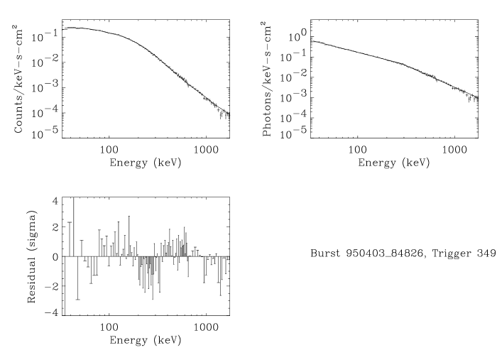
Let us now compare with the corresponding results for the time integrated spectra. As an example in Fig. 7 we report the peak spectrum of the trigger 2083. Comparing with Fig 5 (showing the spectrum time integrated over the whole peak, for trigger 4392) it is evident that the time resolved spectra better constraint the best fitting model: in fact (for example in this case) the time averaged pulse spectrum was satisfactorily fitted by all the 4 models whereas the peak time resolved spectrum is not well fitted by the SSM model because the low energy powerlaw spectral index is fixed at -2/3 and the spectrum is harder than this slope ($\alpha=-0.03\pm 0.06$ for the BAND model). In this example the BAND, COMP and BPLW model provide the best fits and among them the BAND model has the best $\chi^{2}_{red}=0.99$.

This represents a clear indication that the time resolved spectra have to be used in determining the spectral properties of GRBs: average spectra can be effective in comparing the global properties of different bursts, but the actual spectral shape requires high temporal resolution data.

Refer to captionRefer to caption

Refer to captionRefer to caption

Refer to captionRefer to caption

Refer to captionRefer to caption

Figure 7: Trigger 2083. Spectral fits to the pulse peak spectrum. The spectrum is integrated over the time interval [1.088-1.216] sec since the trigger time. The model fits and the residuals are for the BAND, BPLW, SSM and COMP model displayed clockwise starting from the top left corner.
Refer to caption
Figure 8: Reduced $\chi^{2}$ distributions for the 4 spectral models. The total number of time resolved spectral fits is 700 for the BAND and BPLW (dotted and solid line top panel) and COMP and SSM (solid and dot–dashed line bottom panel).

4.2.3 Spectral parameters distributions

In this Section we consider the distribution of the model parameters as inferred from the time resolved data, compare again the different models,and compare these results with the time integrated ones and with previous findings.

  • The low energy spectral component.

    The BAND, COMP and BPLW fits are comparable at low energies as shown by the corresponding $\alpha$ distributions presented in fig. 9: the BAND and COMP model distributions are similar, as in the case of the time integrated spectra, and both have a mode of $-0.85\pm 0.1$, consistent at $2\sigma$ with the BPLW average value $-1.15\pm 0.1$. Note that qualitatively the extension of the $\alpha$ distribution of the BPLW model towards lower values could be attributed to the fact that at low energies the sharp break tends to underestimate the hardness of the spectrum compared to a smoothly curved model.

    The average low energy spectral slope obtained from the time resolved spectra is harder than what obtained with the time integrated pulse spectra for all the three models (BAND, BPLW, COMP). This is a consequence of time integration (i.e. hardness averaging) of the spectral evolution (which can be also very dramatic) over the entire rise and/or decay phase of the pulse.

    Refer to caption
    Figure 9: Low energy power law spectral index ($\alpha$) distributions derived from the time resolved spectral analysis. Solid line: BPLW model, dotted line: BAND model, dashed line: COMP model. The vertical line represents the synchrotron limit ($\alpha=-2/3$) for the low energy spectral shape.

    Even though we present the spectral analysis with 4 models separately we can compare these results with those obtained by Preece et al. (Preece2000 (2000)), where they considered the low energy spectral index distribution regardless of the (best) fitted model. We obtain a similar distribution but with a harder average low energy spectrum ($\alpha\sim-0.85\pm 0.1$ considering the BAND and COMP model, to be compared with $\sim-1.05\pm 0.1$). This difference might be a consequence of the fact that we are considering a subsample of that of Preece et al. (Preece2000 (2000)), including only the bright GRBs which might be intrinsically characterized by a harder spectrum (Borgonovo & Ryde Borgonovo (2001)) and because we restricted our time resolved spectral analysis to the peak interval excluding the inter-pulse phase of multi-peaked events.

  • The high energy spectral component.

    In many spectra the steepness of the count distribution above the break energy $E_{0}$, coupled with the poor S/N ratio, result in a poorly determined value of $\beta$. This is true especially in the case of the BAND model: when the break energy $E_{0}$ sets at high values the exponential roll–over leaves too few high energy spectral channels free for fitting the $E^{\beta}$ component properly. In Fig. 10 we report the BPLW, BAND and SSM $\beta$ distributions. Also in this case the BPLW model, due to its sharpness, tends to overestimate the hardness of the count spectrum giving systematically higher values of $\beta$ than the BAND model. The mode of this parameter is $-2.45\pm 0.1$ and $-2.05\pm 0.1$ for the BAND and BPLW model, respectively.

    The SSM average $\beta$ is $-2.17$ which is consistent with what found from the average pulse spectral analysis. The average $\beta$ value for the BAND model ($-2.45\pm 0.1$) is softer than the time averaged results, and the BPLW model value ($-2.05$) is consistent with the results of Table. 3.

    In fig. 10 it is also indicated the critical value $-2$: spectra with $\beta\geq-2$ are rising in $EF_{E}$, and we can set only a lower limit to $E_{peak}$. These cases correspond to the 18% and 7% of the spectra fitted with the BAND and BPLW model and the 16% for the SSM. Notice that there is also a subclass of soft-spectra with $\beta\leq-3$ which are characterized by a very steep spectral tail: these spectra are clearly better fitted by the COMP model.

    The spread in these $\beta$ distributions ($-4\leq\beta\leq-1.5$) corresponds to what found by Band et al. (Band b (1993)).

    Refer to caption
    Figure 10: High energy power law spectral index ($\beta$) distributions for the time resolved spectra. Solid line: BPLW model; dotted line: BAND model; dot–dashed line: SSM model, in this case $\beta$ is calculated from the $\delta$ parameter (see text). Also shown (bin with $\beta$=-5) the time resolved spectra with undetermined high energy spectral index for the BAND model. The dashed vertical line indicates the critical value $\beta=-2$.
  • The spectral break.

    The most important spectral parameter obtained in fitting the spectrum with these models is $E_{peak}$. As just mentioned this characteristic energy can be obviously calculated only for those spectra (BPLW and BAND model) with $\beta<-2$.

    Refer to caption
    Figure 11: Peak energy distribution for the 4 spectral models. solid line: BPLW model, dotted line: BAND model, dashed line: COMP model, dot–dashed line: SSM model. Spectra with undetermined peak energy (i.e. the high energy threshold 1800 keV assumed as lower limit) are reported in the last bin.

    In Fig.11 the peak energy distributions for the various models are reported and it is also shown the bin with $E_{peak}$=1800 keV, assumed as lower limit of the peak energy for those spectra in which the BAND, BPLW or SSM model have $\beta\geq-2$.

    The mode is $E_{peak}=280^{+72}_{-57}$ keV for the BAND model, consistent, within its error bar, with the BPLW most probable value of $211^{+25}_{-22}$ keV. The COMP model, instead, gives a highly asymmetric peak energy distribution with a mode of $595^{+104}_{-88}$ keV because the lack of a high energy power law component tends to overestimate the energy corresponding to the start of the exponential cutoff. The SSM model has an average $E_{peak}\sim 316^{+64}_{-52}$ keV with a wide distribution.

    From the analysis of the average spectral shape, obtained from the time integrated and from the time resolved spectral analysis, we would like to stress that if we want to characterize the spectral hardness it is necessary to extend the single parameter analysis, typically based on the peak energy or the hardness ratio, and consider the low and high energy spectral components.

Refer to caption
Figure 12: Trigger 2083. Spectral evolution of the BAND model parameters fitted to the time resolved spectra. Light curve on the 64ms time-scale (panel a) for the energy range 110–320 keV (corresponding to channel 3 of the detector); low energy spectral index and (dashed) synchrotron shock model limit $\alpha=-2/3$ (b); peak energy (c). For reference the average values of $\alpha$ and $E_{peak}$ obtained from the time resolved spectra (dotted line) and the synchrotron model limit (dashed line) are reported.

4.3 The Synchrotron limit violation

A well known prediction of the optically thin synchrotron model is that the asymptotic low energy photon slope $\alpha$ should be lower than or equal to $-2/3$ (Katz et al. Katz (1994)). From the analysis of the time resolved spectra we obtain that not only the low energy power law slope can violate this limit, but it can also evolve dramatically during a single pulse (as already found by Crider et al. 1997a ,b).

Refer to caption
Figure 13: Trigger 5614. Spectral evolution of the COMP model fitted to the time resolved spectra. Light curve on the 64ms time-scale panel (a) for the energy range 110–320 keV (corresponding to channel 3 of the detector); low energy spectral index and (dashed) synchrotron shock model limit $\alpha=-2/3$ (b); peak energy (c). For reference are reported the average values of $\alpha$ and $E_{peak}$ obtained from the time resolved spectra (dotted line) and the synchrotron model limit (dashed line).

We can characterize this behaviour, for example, via the BAND and COMP model fits (we exclude the BPLW model which, as showed above, tends to underestimate the hardness of the spectrum at low energies). We obtain that the 14% of the time resolved spectra fitted with the BAND model are inconsistent with $\alpha\leq-2/3$ at 2$\sigma$. A similar percentage ($\sim$11.7% of course mostly for the same spectra) of spectra violating the $\alpha$ limit is found for the COMP model.

For these extremely hard spectra no correlation between $\alpha$ and any other fit parameter is found, and the violation occurs both in the rise and decay phase of the pulses. Moreover $\sim$ 21% of the time resolved spectra corresponding to the peak time bin violate at $2\sigma$ the synchrotron limit, indicating that this violation happens during the peak phase and not preferentially before or after it. As an example in Fig. 12 we show the spectral evolution of $\alpha$ in the case of trigger GRB921207 (BAND model). During the main peak (t$\in$[0.0,4.5] sec) the majority of the time resolved spectra violates the synchrotron model limit (dashed line in panel (c)). Notice that during this time interval the low energy spectral index evolves between $-2/3$ and 0.0 and the peak energy (panel (b)) decreases monotonically. Another interesting example is reported in Fig. 13. GRB960924 shows a low energy spectral shape harder than $-2/3$ only around the peak, and the $\alpha$ evolution during the rise phase covers an interval of $\Delta\alpha\sim 1.4$.

The predictions of the synchrotron model have been recently discussed by Lloyd & Petrosian (Lloyd (2001), L&P2001). They claim that the low energy spectral limit $-2/3$ is not so constraining if (among other assumptions) an anisotropic pitch angle distribution is assumed for the emitting electrons (which should be the case in a low density and intense magnetic field regime). In the case of small pitch angles ($\Psi\ll 1$) the emitted spectrum should be characterized by three components: a low energy flat count spectrum $\nu^{0}$ (for $\nu\ll\nu_{s}\equiv 2/3\ \nu_{b}/(\gamma_{m}\ \Psi^{2})$) followed by the typical $\nu^{-2/3}$ power law (for $\nu_{s}\leq\nu\leq\nu_{m}$) and then by $\nu^{-(p+1)/2}$. p is the electron power law energy index, $\nu_{s}$ the break at the transition from the flat spectrum to the $-2/3$ slope, and $\nu_{m}$ represents the frequency corresponding to $\gamma_{m}$ where the electron energy distribution is smoothly cut off (at low energies).

According to L&P2001 $\alpha\geq-2/3$ is allowed and the slope $\nu^{\alpha}$ obtained from fitting a two component model (like the BAND function) to such a three components spectrum is typically an average between $\nu^{0}$ and $\nu^{-2/3}$. During the emission the electrons cool so that their low energy limit $\gamma_{m}$ decreases and as a consequence the peak energy becomes softer $E_{peak}\propto\gamma_{m}^{2}$. The electrons average pitch angle decreases (although their distribution can be still anisotropic) and this causes the frequency $\nu_{s}\propto(\gamma_{m}\ \Psi^{2})^{-1}$ to increase. The spectral evolution predicted by this model then is of hardening of the low energy powerlaw – because of the progressive disappearance of the $\nu^{-2/3}$ spectral component – while the peak energy naturally evolves from hard to soft. Thus in burst violating the synchrotron limit, a negative correlation between the peak energy and the low energy spectral index is expected.

We report in Fig. 14 as an example the evolution during GRB 920525 which shows a low energy spectral component harder than $-2/3$ during the main peak (for $\sim$ 2 sec). We note (panel (b) and (c) in Fig. 14) that there is no evidence for negative correlation between the peak energy and $\alpha$: during the rise phase of the flux (panel (a)) the peak energy increases regardless of the rise and partial decay of the spectral index, while for the rest of the pulse the peak energy decreases and alpha varies above the $-2/3$ limit. The same happens for GRB 921207 (Fig. 12) and GRB 960529 (Fig. 15): in these bursts the peak energy decreases while $\alpha$ goes above and below the synchrotron limit.

Refer to caption
Figure 14: Trigger 1625. Spectral evolution of the BAND model parameters fitted to the time resolved spectra. Light curve on the 64ms time–scale (panel a) for the energy range 110–320 keV (corresponding to channel 3 of the detector); low energy spectral index and (dashed) synchrotron shock model limit $\alpha=-2/3$ (b); peak energy (c).
Refer to caption
Figure 15: Trigger 5477. Spectral evolution of the BAND model parameters fitted to the time resolved spectra. Light curve on the 64ms time-scale (panel a) for the energy range 110–320 keV (corresponding to channel 3 of the detector); low energy spectral index and (dashed) synchrotron shock model limit $\alpha=-2/3$ (b); peak energy (c).

5 Conclusions

We considered a sample of bright bursts detected by BATSE and performed a uniform analysis for the time integrated and the time resolved (typically 128 ms) spectra with four different models proposed in the literature.

We find that even with this time resolution no parametric model can better represent the data and different spectra require different shapes, re–confirming the erratic behaviour of bursts and also possibly indicating that time resolution on time–scales comparable with the variability one is needed to shed light on such erratic characteristics.

Indeed, an important result we confirm is that the average time integrated spectrum often used in the literature does not well represent the very same event resolved on shorter time-scales. The time integrated spectra might still be used for a comparison of the average spectral shape among different pulses and as indicators of the average spectral parameters of the time resolved analysis although only the time resolved spectra should be used in any test of a physical emission model.

Finally, a considerable number of the fitted spectra are characterized by extremely hard low energy components with spectral index $\alpha$ greater than $-2/3$, value predicted by synchrotron theory (Katz Katz (1994)). This violation was found by Crider et al. (1997a ) and has been recently reported by Frontera et al. (Frontera (2000)) in some GRBs observed by BeppoSAX. They report 1 sec time resolved spectra significantly harder than $E^{-2/3}$, mainly during the first phase of the burst emission. We have found that in 11 of the 25 bursts analyzed the $\alpha$ limit violation is evident mainly in the spectra around the peak both during the rise and decay phase, and this could indicate that at least at some stages of the burst evolution – possibly near the peak of emission itself – radiative processes, other than synchrotron, can dominate the emission.

We also reported some examples of bursts which violate the synchrotron limit and are not characterized by the $\alpha$ $E_{peak}$ anticorrelation predicted by the small pitch angle distribution synchrotron model proposed by Lloyd & Petrosian (Lloyd (2001)).

The obvious extension of this work, namely the study and discussion of the temporal evolution of the spectral shape, will be the subject of a forthcoming paper (Ghirlanda et al., in preparation).

Acknowledgements.
This research has made use of data obtained through the High Energy Astrophysics Science Archive Research Center Online Service, provided by the NASA/Goddard Space Flight Center. We are grateful to D. Band for useful discussions and suggestions for the BATSE data analysis and then for his careful reading of the manuscript and useful comments on it as referee. We are also grateful to M. Tavani for providing his code for the SSM model. Giancarlo Ghirlanda and AC acknowledge the Italian MIUR for financial support.

References

  • (1) Band D. L., Ford L. A., Matteson J. L., 1992, Experimental Astronomy, 2, 307
  • (2) Band D. L., Matteson J. L., Ford L. A., 1993, ApJ, 413, 281
  • (3) Borgonovo L. & Ryde F., 2001, ApJ, 548, 770
  • (4) Crider A., Liang E. P., Smith I. A., 1997, ApJ 479, L39
  • (5) Crider A., 1997, AIP Conference series 428, Gamma Ray Bursts: 4th Huntsville Symposium, ed. Meegan C. A., pp.359-363
  • (6) Epstein R. I., 1973, ApJ, 183, 593
  • (7) Fenimore E. E., 1999, ApJ, 518, 375
  • (8) Fishman G. J., 1989a, in Proc. Gamma Ray Observatory Science Workshop (Washington:NASA),3-47
  • (9) Fishman G. J. & Meegan C. A., 1995, ARA&A, 33, 415
  • (10) Fishman G. J., Meegan C. A., Wilson R.B., 1994, ApJS, 92, 229
  • (11) Ford L., 1993, A Guide to the Spectroscopic Oriented Analysis Routines version 2.1
  • (12) Ford L. A., Band D. L., Matteson J. L., 1995, ApJ, 439, 307
  • (13) Frontera F., Amati L., Costa E., 2000, ApJ, 127, 59
  • (14) Katz J.I., 1994, ApJ 432, L107
  • (15) Kennel C. F. & Coroniti F. V., 1984, ApJ, 283,694
  • (16) Kitchin C. R., 1991, Astrophysical Techniques 2nd ed., Adam Hilger
  • (17) Liang E. P. & Kargatis V. E., 1996, Nature, 318, 495 
  • (18) Lloyd N. M & Petrosian V., 2001, astro-ph/0109342
  • (19) Matz S. M., Forrest D. J., Werstand W. T., 1985, ApJ, 288, L37
  • (20) Mazets E. P., Golenetskii S. V., Gurian Iu. A., 1982, Ap&SS, 82, 261
  • (21) Meegan C. A., Pendletn G. N., 1996, ApJS, 106, 65
  • (22) Paciesas W. S., Meegan C. A., Pendleton G. N., 1999, ApJS, 122, 465
  • (23) Preece R. D., Briggs M. S., Mallozzi R. S., 2000, ApJS, 126, 19
  • (24) Preece R. D., Pendleton G. N., Briggs M. S., 1998, ApJ, 496, 849
  • (25) Preece R. D., Briggs M. S., Pendleton G. N., 1996, ApJ, 473, 310
  • (26) Rees M. J. & Meszaros P., 1994, ApJ, 430, L93
  • (27) Rybicki G. B. & Lightman A. P., Radiative Processes in Astrophysics, New York: Wiley 1979
  • (28) Ryde F., 1999, Astro Lett. & Communications , 39, 281
  • (29) Tavani M., 1996, ApJ, 466, 768